Mawrth Vallis, Mars, classified using the NOAH-H deep-learning terrain classification system

ABSTRACT

A deep learning (DL) terrain classification system, the Novelty and Anomaly Hunter – HiRISE (NOAH-H) was used to produce a terrain map of Mawrth Vallis, Mars. With it, we digitised the extent and distribution of transverse aeolian ridges (TARs), a common type of martian aeolian bedform. We present maps of the site, classifying terrain into descriptive classes and interpretive groups. TAR density maps are calculated, and the network output is compared to a manually produced map of TAR density, highlighting the differences in approach and results between these methods. Even when mapping on a small scale, humans must divide the terrain into coherent patches in order to map a large area in a reasonable time frame. Conversely, the speed of DL systems enables mapping on the pixel scale, producing a more detailed product, but one which is also “noisier”, and less immediately informative. There are pros and cons to both approaches.

Highlights

• A morphological map of Marth Vallis, Mars, has been created, classifying variations in surface texture into 14 descriptive classes.

• A deep learning (DL) convolutional neural network was trained to predict these classes in further HiRISE images, which had not been used for training.

• The resulting classified rasters were orthorectified and mosaicked using ArcGIS.

• Appropriate classes from the resulting map were compared with manual digitisation of the spatial densities of Transverse Aeolian Ridges (TARs).

• This comparison highlights the different scales at which human and DL mapping takes place, and that the two datasets have different strengths and weaknesses.

• The speed at which the network can complete its task allows it to attempt a higher level of fidelity than is possible for a human.

• Derived maps of the density of boulders and TARs were also produced using both the DL and manual datasets.

KEYWORDS:

• Mars
• machine learning
• Mawrth Vallis
• ExoMars

1. Introduction

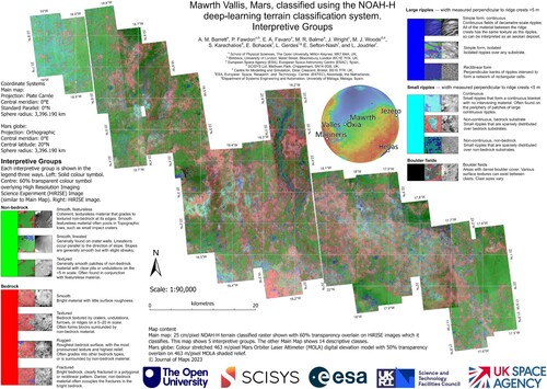
We present a terrain map of Mawrth Vallis, Mars, showing the distribution of aeolian bedforms and classifying surface texture type (Main Map sheets 1 and 2). Our classification ontology was designed with rover traversability in mind, as part of the landing site selection process for the European Space Agency (ESA) Rosalind Franklin Rover mission (ExoMars, Loizeau et al., 2019; Vago et al., 2017). This is the third in a series of maps presenting the results of the Novelty and Anomaly Hunter – HiRISE (NOAH-H) study (Barrett et al., 2022b; Wright et al., 2022). NOAH-H is a deep learning (DL) convolutional neural network designed to classify the surface of Mars into 14 textural classes (Barrett et al., 2022a; Woods et al., 2020). The network classifies satellite images from the High-Resolution Imaging Science Experiment (HiRISE) instrument. We used red-band images with 25 cm/pixel resolution (McEwen et al., 2007). The NOAH-H network was trained on data from Oxia Planum (e.g. Fawdon et al., 2021; Quantin-Nataf et al., 2021) and Mawrth Vallis (e.g. Loizeau et al., 2019; Poulet et al., 2020), the final two candidate ExoMars landing sites under consideration at the time the DL system was devised (Vago et al., 2017).

In Barrett et al. (2022b), we published our map of the selected landing site in Oxia Planum, Mars. For Oxia, no large-scale human-made map is yet available for comparison. However, the DL classified masks were a good qualitative match for landscape-level trends visible in HiRISE images. The network demonstrated a high mean Intersection over Union (IoU) when comparing the portion of the training data reserved for validation (Barrett et al., 2022a) giving us confidence in the results of the classification.

In Wright et al. (2022), we presented results for Jezero Crater, Mars, the landing site of NASA’s Perseverance Rover (Farley et al., 2020). Here we compared our results to manual mapping of the site conducted by the Perseverance team (Stack et al., 2020) as well as to in situ observations from both the rover and the Ingenuity helicopter (Balaram et al., 2021). While the mapping of Stack et al. (2020) was conducted by a different team, using very different categorisations, our comparison at Jezero Crater was broadly favourable. We were able to match up their work with ours in broad terms, although we were hampered by the difference in mapping scale. This suggests that our model is fit for purpose when predicting broad, landscape-level trends. Since Jezero Crater was not a source of training data, this also demonstrates transferability of the model to similar regions of Mars.

Here we present our work characterising Mawrth Vallis. This area was studied intensively as part of the ExoMars landing site selection process. Part of that analysis included identifying and mapping transverse aeolian ridges (TARs); TARs represent a substantial rover traversability hazard (Balme et al., 2018a), and their mapping constituted an important consideration for ensuring the success of the rover mission. These TARs were mapped over a large area at a map scale of between 1:5000 and 1:10,000 i.e. the HiRISE image was zoomed out by a factor of 3 relative to native resolution, and the mapping aimed for fidelity on a scale of ∼10 m. We compared this manual mapping to the DL classification, over an entire HiRISE image (ESP_046459_2025), to see what differences and similarities there are between the two products.

The comparison is still not entirely like-for-like, since the manually mapped dataset was completed prior to the NOAH-H training and did not specifically use our classification scheme. However, it did break down the bedform patterns into continuous and discontinuous areas. This makes it more comparable to the DL-produced product than other available datasets and yields valuable insights into the pros and cons of the two mapping approaches.

2. Study area

Mawrth Vallis is ‘the landing site that wasn’t’; it has nearly been selected as the destination of multiple Mars rover missions. It was a finalist for the ESA Rosalind Franklin rover, and was considered for both NASA’s Perseverance and Curiosity missions (Michalski et al., 2010; Poulet et al., 2020). It remains of great scientific interest, despite being a challenging landing site from the perspective of geological context and traversability constraints. The region is shown in Figure 1.

Figure 1. Map of the Mawrth Vallis study area, showing the region on the southern bank of the valley where classification was conducted. The area classified using the Machine Learning approach is outlined in black, while the area mapped by a human is outlined in red. Basemaps: HRSC HMC_11E10_co5 (Gwinner et al., 2016) one of the instruments which first detected clays at Mawrth, Mars Global MOLA digital elevation model (Smith et al., 2001).

The deep learning classified area is irregularly shaped, corresponding to the footprints of overlapping HiRISE images. It is 15,000 km long, and 500 km wide (at its widest point). The human mapped area is smaller, only 500 by 500 km, and falls almost entirely inside the middle of the deep learning classified area. A Mars globe shows that Mawrth Vallis is located on the edge of Chryse Planitia, near to Oxia Planum, but further away from Jezero Crater where our other mapping studies have taken place.

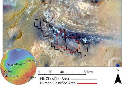
The proposed landing site for the ExoMars mission was located on the planetary dichotomy boundary, where the highlands of Arabia Terra give way to the low, flat terrain of Chryse Planitia. The region of interest is a series of plateaus along the southern side of the Mawrth Vallis channel. These have been heavily eroded, exposing layered rocks which contain a record of several ancient aqueous environments (Loizeau et al., 2012; Michalski et al., 2010). Their context and good state of preservation make them a useful site for investigating the habitability of early Mars (Poulet et al., 2020). The rocks at Mawrth Vallis probably date from the early Noachian to the early Hesperian epochs, and so record periods of relatively warm and wet conditions on early Mars. Consequently, the hydrated silicates in the stratigraphy at Mawrth Vallis represent the environment from a time when Mars was most habitable.

3. Methods

3.1. NOAH-H classification

The procedure by which the NOAH-H system was trained to classify martian surfaces has been described in detail in Barrett et al. (2022a). In brief, 1500 small sections of HiRISE images (‘framelets’) were annotated with expert labels. Terrains were classified on a pixel scale, by drawing over the image in a labelling tool to classify areas of the image into one of 14 ontologies. Although a vector tool was used to classify blocks of pixels, the classification was raster based. These masks were then used to train and validate the network, which was based on a modified version of the algorithm ‘deeplab’ (Chen, 2017). Half of the framelets used to train the network were from Mawrth Vallis, with the rest from Oxia Planum. The classification scheme is described in Table 1 and in the legends of the two main map sheets, where type examples are shown. For more detail on how the classification scheme was developed and applied see (Barrett et al., 2022a).

Table 1. Overview of the NOAH-H classification scheme (Barrett et al., 2022a).

Notes: The ontology has two levels: (i) descriptive classes and (ii) interpretive groups. The RGB values used to classify these classes and groups throughout this study are given.

Qualitative evaluation of the images was conducted to assess how well they conformed to the terrain seen by experts in the HiRISE data (Barrett et al., 2022a) the model was found to perform well on a landscape level. Unlike our analysis of Jezero Crater, this study does not involve transferring the model to a new site, and so many of the misclassifications seen there are avoided. The data for Mawrth was thus expected to be of a comparable quality to that used for the Oxia Planum map (Barrett et al., 2022b).

The method by which images were georeferenced and mosaicked to produce our final classification products are detailed in Barrett et al. (2022b) and Wright et al. (2022). An identical procedure was conducted here. In brief; the original HiRISE images were loaded into ArcGIS Pro, and georeferenced to a basemap (HRSC image HMC_11E10_co5 (Gwinner et al., 2016)). Several hundred control points were placed on each HiRISE image to tie it precisely to the HRSC data. The image was then orthorectified using a spline transformation. The control points were saved and applied to the classified mask produced by NOAH-H. This was orthorectified using the same transformation as the source HiRISE image. The rectified NOAH-H masks were then mosaicked in ArcGIS, using the procedure outlined in Wright et al. (2022). In regions of overlap the same pixel priorities shown in Table 1 of that paper were used to determine which pixel would be adopted in the final map.

3.2. Preparing the comparison product

In order to characterise the suitability of Mawrth Vallis for investigation by rover, an estimate of the coverage of the site by aeolian bedforms was required. These features, primarily TARs (Balme et al., 2008) could impede the progress of a rover since windblown deposits are generally made of loose, unconsolidated material which provide less grip for rover wheels than solid rock or more coherent regolith (e.g. Balme et al., 2018).

TARs were manually digitised using ArcGIS across the central part of the proposed ExoMars landing site on data available in 2016. Areas covered by aeolian bedforms were digitised using a GIS polygon layer. Polygon feature classes were established indicating whether an area exhibited 100% aeolian cover, 50%, or 20%.

• In a ‘100%’ region TARs are essentially continuous, with no gaps in between.

• Areas recorded as ‘50% coverage’ are densely covered by TARs, which must cover in excess of 50% of the region by area. Gaps must be present between some TARs, but are not required between all of them.

• ‘20%’ areas are sparsely covered with an average of 20% coverage. TARs are present, but are rarely contiguous, and the areal extent of aeolian bedforms is substantially less than 50%.

For the purposes of calculating overall aeolian cover, areas can be considered to have at least the coverage with which they are labelled, but no more than the next highest category.

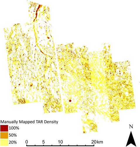
These feature classes where then used to draw around regions of 20% cover, then 50%, and 100% respectively before clipping to preserve the highest digitised density polygon in any given location. This process took approximately 10 working days for an experienced GIS user to cover ∼840 km² (Figure 2).

Figure 2. Manual map of ripple distribution across the central Mawrth area. Patches of bedforms are digitised. Patches with 100% TAR coverage are shown in dark red, while 50% coverage is shown in mid-toned orange, and 20% coverage in pale yellow. Areas with discontinuous coverage (20% and 50%) are much more common than areas with 100% cover. Patches with 100% cover are only seen in a few places, such as the interiors of valleys and craters. 20% coverage areas are more common, but are still not evenly distributed across the area, being generally denser to the northwest of the region. The edges of some HiRISE images correspond to changes in TAR density. This is likely due to the illumination conditions in those images affecting how well the TARs could be resolved. We recommend downloading the online version of this figure, to better see the small details.

A 30 × 30 km area is shown. Patches of TARs have been mapped across the footprints of 8 HiRISE images, which do not quite fill the square. 100% coverage is found in small coherent areas, corresponding to crater and valley floors on the map in Figure 1. Discontinuous TARs are more common but are not uniformly distributed across the area. Bands of denser TAR coverage cross the image diagonally from southeast to northwest. A few changes in density correspond to the edges of HiRISE images.

4. Results

Terrain classification by NOAH-H at Mawrth Vallis matches well with manual interpretations (Barrett et al., 2022a). Comparing NOAH-H results to the 10% of training framelets reserved for validation yielded a mean Intersection over Union (IoU) of 74.15% when predicting descriptive classes; the full list of 14 ontologies that describe the textural characteristics of the surface or bedforms. An IoU of 92.33% was yielded when first-level aggregation was used to combine these textural classes into ‘interpretive groups’; broader thematic groupings indicative of certain formation mechanisms (bedrock vs non-bedrock etc). These metrics, combined with qualitative comparison of the product to the original HiRISE suggest that NOAH-H is fit for purpose. Figure 3 compares NOAH-H classification to the original HiRISE and manual map. Figures 4 and 5 show the main map sheets for descriptive classes and interpretive groups, respectively.

Figure 3. Example of a classified area of HiRISE ESP_046459_2025_RED, classified into descriptive classes: (a) the original HiRISE, (b) the classified mask produced by the NOAH-H network, (c) Manually Mapped TAR density, (d) NOAH-H TAR classes, symbolised in the same way as the manual map. The manual map consisted of three density classes, represented by red, orange and yellow for 100%, 50%, and 20% respectively. The ML only predicts 100% and 20% classes, so only red and yellow appear in inset d.

Four maps of the same 1.3 km by 2 km area illustrate that the machine learning system does a good job of identifying key features of interest, in particular Transverse Aeolian Ridges (TARs), and rugged bedrock areas. The map showing the HiRISE image shows dark toned non-bedrock areas contrasting with bright toned bedrock and ripples. These bright areas have been segmented in the map showing the classified mask, distinguishing them from the non-bedrock material. The human-made map shows large coherent patches, classified as continuous or discontinuous, the NOAH-H map shows the same pattern, but with much more detail, as individual TARs have been outlined.

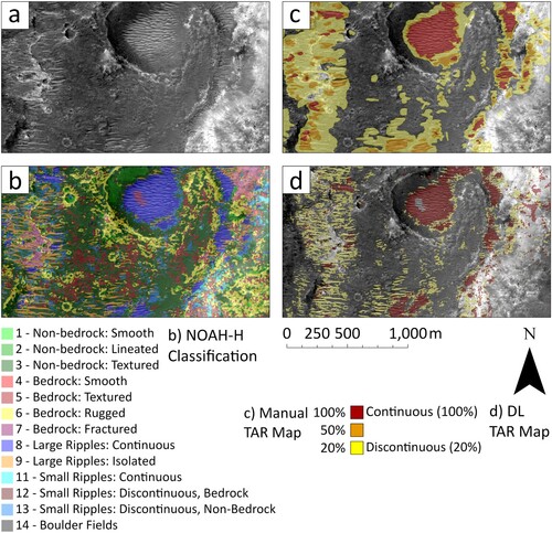
Figure 4. Main map of Mawrth Vallis, showing descriptive classes. GIS-ready files are available as supporting material and we encourage readers to download these in order to view the product at full resolution and symbolise it as needed to better highlight the more subtle variations.

A coloured map shows descriptive classes across the whole study area. Bedrock predominates in several blocks, corresponding to rocky plateaus, while more non-bedrock is seen in the channels and valleys in between. Concentrations of aeolian cover are seen in the far northwest of the map, and within the valleys. The map key shows a swatch of each colour, alongside a type example of the class.

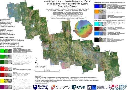
Figure 5. Main map of Mawrth Vallis showing interpretive groups. GIS-ready files are available as supporting material and we encourage readers to download these in order to view the product at full resolution and symbolise it as needed to better highlight the more subtle variations.

A coloured map shows interpretive groups across the whole study area. As with Figure 4, bedrock predominates in several blocks, corresponding to rocky plateaus, while more non bedrock is seen in the channels and valleys in between. Concentrations of aeolian cover are seen in the far northwest of the map, and within the valleys. The map key shows a swatch of each colour, alongside a type example of the class.

A 500 m diameter crater fills the upper right-hand side of Figure 3. Its rim and the rocky ground that surrounds it are marked ‘rugged bedrock’ by the network. The crater floor is filled with non-bedrock material and a large patch of TARs, as is the area to the south of the rim. The crater interior and a north–south trending band to the east contain TAR patches, which have been correctly identified as ripple classes. Areas of small and large continuous ripples are well-defined, and these are interleaved with examples of large, isolated ripples. A few patches of bedrock are detected, but these are primarily visible beneath areas of textured non-bedrock material. In insets c and d, NOAH-H has classified TARs in generally similar areas to the human mapper, however the NOAH-H output segments individual bedforms, while human mapping groups areas of TARs in 100-1000 m scale patches. This means that while the trends are the same, there are many gaps in the classification, where a non-ripple class has correctly been identified in a space in which the human mapper included in the discontinuous unit.

5. Analysis & discussion

5.1. Comparison of DL classification to manual mapping

It is important to validate the results of machine learning classification against preexisting human-made products. However, such comparisons are rarely completely like for like. This can limit the applicability of certain traditional metrics such as precision and recall. In the following section we provide details of the comparison between our two datasets, and highlight some of the important considerations when conducting analyses of this sort.

HiRISE image ESP_046459_2025 was selected to compare NOAH-H and manual classifications. It exhibits a variety of aeolian bedforms and is central to both human and NOAH-H classified areas. All analysis was conducted using ArcGIS Pro software. The manually digitised TAR patterns were converted to a raster dataset with a resolution of 10 m/pixel as this best reflected the fidelity of the manual mapping. ‘Snap raster’ was used to align the pixels of this new raster to those of the NOAH-H mosaic, allowing for a direct comparison of the two. The NOAH-H mosaic was then down-sampled to the same resolution, using a ‘majority’ approach so that each new 10 m pixel represented the mode of the 1,600 25 cm pixels which composed it. Both datasets were clipped to the extent of the HiRISE image. Down-sampling smooths out some of the pixel-scale ‘noise’ in the NOAH-H data, which does not reflect real, landscape-scale, variations in surface texture but would affect the comparison.

The manually mapped TARs consist of three classes: 100% coverage, 50% coverage, and 20% coverage. The 100% class is considered to correspond to NOAH-H classes 8, 10 and 11, and are termed ‘Continuous TARs’. The distinction between the 20% and 50% classes is not reflected in the NOAH-H classification system, so these two classes were aggregated into a single ‘Discontinuous TARs’ class. This corresponds to NOAH-H classes 9, 12, and 13.

Using the ‘reclassify’ tool the two datasets were converted into Boolean masks showing the presence or absence of a class. Three masks were produced for each dataset: all TARs, Continuous TARs, and Discontinuous TARs. Difference plots were computed using the ‘compute change raster’ tool, with the manual observations set as the ‘from raster’, and the DL classification as the ‘to raster’. This allows us to differentiate between type I and type II errors. (1) $\mathrm{D}\mathrm{i}\mathrm{f}\mathrm{f}\mathrm{e}\mathrm{r}\mathrm{e}\mathrm{n}\mathrm{c}\mathrm{e}=\left(\mathrm{t}\mathrm{o}\mathrm{r}\mathrm{a}\mathrm{s}\mathrm{t}\mathrm{e}\mathrm{r}\right)-\left(\mathrm{f}\mathrm{r}\mathrm{o}\mathrm{m}\mathrm{r}\mathrm{a}\mathrm{s}\mathrm{t}\mathrm{e}\mathrm{r}\right)$(1) Therefore:

• False positives (type I errors) are objects which are found in the classification, but not in the manual map. These appear as ‘positive changes’ or +1 in the difference map.

• False negatives (type II errors) are objects which are present in the manual map, but not in the classification. These appear as ‘negative changes’ or −1 in the difference map.

The graphical results are shown in Figure 6. Confusion matrices (Table 2) summarise the number of true positives, false positives, and false negatives. Three derived metrics can also be calculated: (2) $\mathrm{R}\mathrm{e}\mathrm{c}\mathrm{a}\mathrm{l}\mathrm{l}=\mathrm{T}\mathrm{P}/\left(\mathrm{T}\mathrm{P}+\mathrm{F}\mathrm{N}\right)$(2) (3) $\mathrm{P}\mathrm{r}\mathrm{e}\mathrm{c}\mathrm{i}\mathrm{s}\mathrm{i}\mathrm{o}\mathrm{n}=\mathrm{T}\mathrm{P}/\left(\mathrm{T}\mathrm{P}+\mathrm{F}\mathrm{P}\right)$(3) (4) $\mathrm{I}\mathrm{o}\mathrm{U}=\mathrm{T}\mathrm{P}/\left(\mathrm{T}\mathrm{P}+\mathrm{F}\mathrm{P}+\mathrm{F}\mathrm{N}\right)$(4) where: True Positive (TP) = Number of pixels correctly classified, False Positive (FP) = Number of pixels incorrectly classified, and False Negative (FN): Number of pixels incorrectly not classified.

Figure 6. Map showing comparison of TAR features to the manual mapping. (a) original HiRISE image ESP_046459_2025. (b) All TARs; manually mapped distribution (yellow), (c) All TARs; deep learning prediction (green), (d) All TARs; difference map (false negatives blue, false positives red). (e) Continuous TARs; manually mapped distribution (yellow), (f) Continuous TARs; deep learning prediction (green), (g) Continuous TARs; difference map (false negatives blue, false positives red). (h) Discontinuous TARs; manually mapped distribution (yellow), (i) Discontinuous TARs; deep learning prediction (green), (j) Discontinuous TARs; difference map (false negatives blue, false positives red). This figure contains very small details, we recommend consulting the online version of the figure in order to examine it at full resolution.

Three images are shown for each of the three cases. The first shows the human map, the second the DL generated map, and the third highlights the differences between them. For All TARs the human and DL maps match in broad trends, but differ in small details. The DL has mapped much more small variation than the human. The other cases show much more dramatic differences. The DL has found far more continuous TARs than the human, but far fewer discontinuous ones. The difference maps thus show lots of false positives for continuous TARs, and lots of false negatives for discontinuous ones.

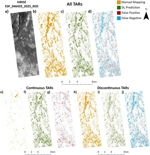
Table 2. Confusion Matrices showing the precision, recall and IoU metrics for each comparison pair.

Thus, precision is a measure of how many of the DL predictions are correct, recall of how many of the ‘ground truth’ features were detected, and IoU is a summary of the two.

Table 2 shows that the model does not reliably replicate the human map. Precision and recall are high for the background class but vary greatly for the TAR Class. Continuous TARs show high recall, but low precision, while the reverse is true for discontinuous features. When all TARs are considered, both metrics are middling. When both classes are considered, most of the confusion is between each class and the background, rather than between continuous and discontinuous.

If this test is taken as a blind measure for fitness of purpose, then this is not a good result. However, using the difference plots, we can clearly pinpoint how and why the two diverge and see that this poor result reflects a systemic difference in classification approach rather than inaccuracy in the model.

In general, the continuous class performs better than the discontinuous. This should be unsurprising, since in the continuous case the network classifies the terrain into large coherent patches. Where discontinuous terrains occur we had to digitise patches of discontinuous cover, rather than individual features, in order to complete the mapping in a reasonable period. The speed at which NOAH-H can complete its task allows it to attempt a higher level of fidelity than is possible for a human. However, this complicates assessing whether the model’s actual performance is good enough to warrant these ambitions. In many ways, the human- and AI-produced datasets will never be entirely comparable.

When all TARs are considered, the overall trend appears similar at first glance. However, NOAH-H has captured much more detail than the human mapper. The result is many small-scale variations, which reduce the accuracy of the classification relative to ‘ground truth’. In the case of continuous and discontinuous TARs, there are major differences between the two products.

The DL map has captured far more continuous TARs than the human one, whereas the human map captures more discontinuous TARs. In the human map, TARs were only digitised at all where we deemed their spatial density to be >20%. This is a subjective distinction, and leaves isolated TARs unmapped, however, the DL system can classify every pixel and as such captures many more small and isolated pixel clusters overlooked by the humans. The reverse is true when considering discontinuous TARs. The coherent areas classified as 20% or 50% coverage include many gaps between the bedforms. The DL system has attempted to exclude each of these gaps from its digitisation, classifying them as underlying bedrock or non-bedrock material.

The key questions thus become; are these small-scale variations ‘real’, making for a reliable product, and are they useful to capture? The human product arguably has less fidelity at very small spatial scales, however, it is much clearer and more intuitive to use. Which is better for a given task will vary depending on the precise science question being addressed. The NOAH-H product, taken on its own, arguably has too much small-scale variability to be useful when considering the whole study area and, as Figure 6 and Table 2 show, this is not entirely smoothed out by down-sampling the data to the same scale as the comparison product.

However, if being used for a small area (e.g. the few 100 m surrounding the location of a putative rover), having this level of granularity in assessment of the aeolian hazard is very useful. Note also that the ‘noisy’ output from NOAH-H is a function of using a direct pixel-based classification approach. It is possible that less noisy outputs could be produced by altering the way we model the classification problem via the ontology and labelling approach or via suitable post-processing. We will consider this in any future work. What we have learned from this study will allow us to reframe our classification approach to achieve more human-usable outputs in future.

Consequently, we believe that the NOAH-H results are fit for purpose, but that its use should not be unchecked by human input. Rather, it provides a rich and detailed starting point, from which a product more akin to the manually prepared map can be derived. A human user can start from the NOAH-H classification, removing false positives, adding in false negatives, and smoothing out the polygons into more useful, coherent, blocks. We find this process much less time-consuming than starting from scratch, and manually digitising every landform. It becomes much easier to estimate TAR coverage within a coherent bedform unit with the DL classified raster to work from, and this will make the estimation of coverage percentages such as those used in the manual map more consistent, especially in cases where the size of a study area necessitates multiple scientists contributing to the mapping. This is how we intend to use the network, and it is already being employed as a starting point for the bedform classes in ongoing mapping work at Oxia Planum soon to be submitted to this journal.

5.2. Ripple density statistics

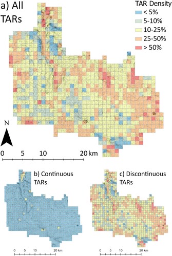
We computed percentage surface cover by TARs using the method described in Barrett et al. (2022b). The NOAH-H and manual mapping rasters were resampled and reclassified into 1 m/pixel Boolean masks, showing the presence or absence of each bedform class; each NOAH-H class was computed separately (figure S1), and they were combined into groups of large, small, continuous, and discontinuous TARs (Figure 7). The manual map was grouped into masks for continuous, discontinuous, and all TARs (Figure 8). The ‘add surface information’ tool was then used to compute ripple density for each square in a 1 km grid, producing a vector output which summarises the density and distribution of aeolian cover for the region. The same procedure was also used on the NOAH-H detections of boulders. Similar to ripples, boulders are a dispersed feature of the landscape, the cover of which has implications for safety of landing and traversing a potential landing site.

Figure 7. Ripple and boulder density statistics derived from the machine learning classification. Coloured grids are overlain on a slope map derived from a CTX stereo mosaic, (a) All TAR classes, (b) all boulders, (c) all large TARs (classes 8–10), d all small TARs (classes 11–13), (e) all Continuous TARs (classes 8–11) and (f) all discontinuous TARs (classes 12–13). Note that for this analysis class 9 has been considered a ‘continuous’ class rather than a discrete one as in the comparison to the manual map. While large, isolated TARs are indeed discontinuous, for the purposes of calculating ripple statistics every pixel classified as class 9 is covered by aeolian material, they thus count towards the total budget of aeolian material at the site, rather than the area covered dispersed features, where each pixel is only ∼20% covered by aeolian material.

Six maps of the study area summarise TAR density for the site. Large TARs cover a slightly larger area than small TARs, and continuous TARs cover a substantially larger area than discontinuous ones. Coverage of small and discontinuous TARs have much the same distribution, with the greatest concentration in the north and west. The inverse is true for large and continuous features, which are found across a much wider area, across the south and east of the site. When all TARs are considered, nearly the entire area has at least 10% coverage, with isolated patches of denser aeolian cover. This is not the case for boulders which are very sparse, with only a few tens of cells exhibiting more than 10% density.

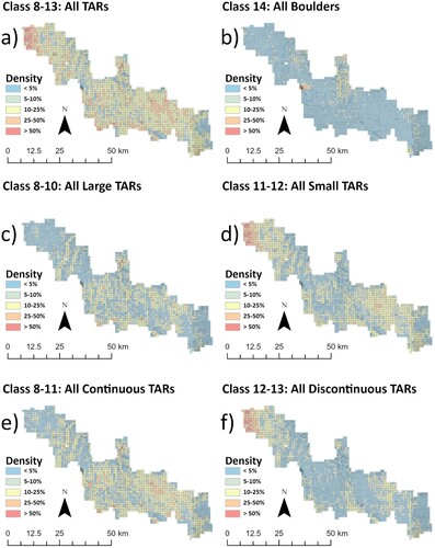
Figure 8. Ripple density statistics derived from the manual mapping. Coloured grids are overlain on a slope map derived from a CTX stereo mosaic. (a) All TARs, (b) Continuous TARs, (c) Discontinuous TARs.

Three maps of the study area summarise TAR density statistics from the manual mapping. There are only 16 continuous TARs cells with more than 5% coverage, and only one cell in the centre north, with more than 25%. These match the small isolated areas seen in Figure 7, The distribution between the All TARs and discontinuous TARs maps is very similar, and shows coverage of between 5 and 50% over most of the area, with isolated regions with low to no coverage. Isolated regions of greater than 50% coverage correspond to valleys and crater floors, and occur in the same areas as those in the NOAH-H version.

In the manually mapped area, 100% TAR coverage is found over a total area of 5.2 x10⁶ m². Discontinuous TARs cover a much larger area, of 2.4 × 10⁷ m² for 50% coverage, and 1.5 × 10⁸ for 20% coverage, respectively. When these areas are adjusted for TAR coverage, manually mapped TARs are found to cover a total area of 4.8 x10⁷ m². When the NOAH-H classified area is clipped to the same extent we find a total of 7.8 × 10⁷ m² of continuous TARs, and 5.2 x 10⁷ m² of discontinuous features. If discontinuous features are weighted at 20% this gives a total of 8.9 × 10⁷ m². This means that the DL approach produces a percentage cover of 10.6%, while the human-mapping yields 5.8% coverage. Despite larger blocks being digitised, and more background material being included, the human map still provides a lower estimate of aeolian cover, due to the vast number of small areas which NOAH-H digitises, which were not significant enough to be included in the human map.

The first thing to note when comparing the ripple density statistics derived from the two methods is that it has been possible to classify a much larger area using the machine learning approach. While the distribution of ‘All TARs’ is similar, this is not the case for the continuous and discontinuous datasets. Relatively few continuous TARs were mapped in the human dataset, and they occur in small patches which do not result in significant coverage at the 1 km grid scale. The reverse is true of the discontinuous features, which were somewhat scarce in the DL-derived dataset, but are found much more readily in the human map.

As shown in section 5.1 the differences between the two classifications are on the metre to decimetre scale, and so aggregating them into 1 km bins can suppress or enhance minor differences in the distributions. The distributions are similar, albeit with very different absolute density.

6. Conclusion

This study has produced DL-derived maps of Mawrth Vallis. We demonstrated how these were produced, and how ripple density statistics can be calculated using them. We compare it to a manual TAR map, but find that although the two products appear broadly similar, there are major pixel-scale differences between them. These are largely due to how the NOAH-H network classifies images on a pixel-by-pixel basis, producing ‘noisy’ classifications, where it attempts to reproduce every metre scale variation. These small-scale variations are interesting, and upon inspection, seem fairly reliable, but are not useful when classifying the terrain on a landscape level. The model does not produce a one-to-one match to the human data. However, it shouldn’t be expected to, as the human mapping aggregated information at the ∼ 10 m scale while summarising this information into large areas. What NOAH-H does do, however, is capture the same landscape-level trends, and this would provide a valuable first step for producing a simplified, human-verified product. In essence, with the NOAH-H classification as a starting point, it would be much easier and faster to achieve this high level of fidelity in a human-produced map than starting from scratch. This is how the NOAH-H tool is being used henceforth. The TAR classes are already being incorporated into manually produced mapping efforts, where, with some manual verification and modification, they can form a valuable component of regional scale mapping efforts.

Software

We used ESRI ArcGIS Pro 2.8 for co-registration of HiRISE and NOAH-H rasters, NOAH-H pixel prioritisation, and generation of the NOAH-H terrain classification map. NOAH-H is a deep learning semantic segmentation software developed by SciSys Ltd (now part of CGI) for the European Space Agency to aid preparation for the ExoMars rover mission.

Clear credit across the NOAH-H Project

This manuscript was prepared by Barrett, who conducted the NOAH-H labelling campaign as well as the validation and application of the dataset. Barrett and Balme formulated the NOAH-H classification scheme, with input from Fawdon. Balme managed the project along with Sefton-Nash and Joudrier at ESA. The NOAH-H network was developed by Woods, Karachalios, and Petrocelli at SciSys, the work having been commissioned by ESA. NOAH-H masks were processed by Woods, Karachalios, and Petrocelli at SciSys, along with Gerdes, Bohacek, and Sefton-Nash at ESA. They supplied the classified images for all three map papers. Wright developed and applied the GIS based mosaicking strategy, and designed the map layout template used for all three papers. Wright led the Jezero comparison and paper writing and developed many of the workflows used in this paper. Barrett led the preparation of the subsequent map papers using the procedure developed along with Wright. Fawdon prepared the manual comparison dataset, and along with Balme provided insight into both the Mawrth and Oxia landing sites. Favaro produced the gridded TAR density statistics with help from Barrett and Fawdon, and led the scientific utilisation of this aeolian data along with Balme.

Acknowledgements

The HiRISE images discussed in this work are publicly available from https://www.uahirise.org/ and are credited to NASA/JPL/University of Arizona. HRSC images are credited to the European Space Agency; Mars Express mission team, German Aerospace Center (DLR), and the Freie Universität Berlin (FUB). They are available at the ESA Planetary Science Archive (PSA) https://www.cosmos.esa.int/web/psa/mars-express and are used under the Creative Commons CC BY-SA 3.0 IGO licence. We thank all the spacecraft teams who produced this data for their wonderful windows into the geomorphology of Mars.

Disclosure statement

No potential conflict of interest was reported by the author(s).

Data availability

The georeferenced mosaics are available from the Open University’s Open Research Data Online (ORDO) system: doi: 10.21954/ou.rd.22960412.

Additional information

Funding

AMB, JW and MRB acknowledge funding from the UK Space Agency (UKSA) and UK Science and Technology Facilities Council (STFC; grant ST/T000228/1), and a European Space Agency contract (4000118843/16/ NL/LvH1145 – Novelty or Anomaly Hunter (NOAH)). EAF and MRB gratefully acknowledge UKSA funding (ST/T002913/1, ST/V001965/1 and ST/R001413/1). PF acknowledges UKSA funding (ST/W002736/1, ST/L006456/1, ST/V001965/1 and ST/R001413/1). JW and EB acknowledge support from the European Space Agency (ESA) as ESA Research Fellows received during the write-up of this work.

References

- Balaram, J., Aung, M. M., & Golombek, M. P. (2021). The ingenuity helicopter on the perseverance rover. Space Science Reviews, 217(4), 1–11. https://doi.org/10.1007/s11214-021-00815-w
- Balme, M., Berman, D. C., Bourke, M. C., & Zimbelman, J. R. (2008). Transverse Aeolian Ridges (TARs) on mars. Geomorphology, 101(4), 703–720. https://doi.org/10.1016/j.geomorph.2008.03.011
- Balme, M., Robson, E., Barnes, R., Butcher, F., Fawdon, P., Huber, B., Ortner, T., Paar, G., Traxler, C., Bridges, J., Gupta, S., & Vago, J. L. (2018). Surface-based 3D measurements of small aeolian bedforms on Mars and implications for estimating ExoMars rover traversability hazards. Planetary and Space Science, 153, 39–53. https://doi.org/10.1016/j.pss.2017.12.008
- Barrett, A. M., Balme, M. R., Woods, M., Karachalios, S., Petrocelli, D., Joudrier, L., & Sefton-nash, E. (2022a). NOAH-H, a deep-learning, terrain classification system for Mars : Results for the ExoMars Rover candidate landing sites. Icarus, 371, 114701. https://doi.org/10.1016/j.icarus.2021.114701
- Barrett, A. M., Wright, J., Favaro, E., Fawdon, P., Balme, R., Woods, M. J., Karachalios, S., Bohachek, E., Sefton, E., Joudrier, L., Barrett, A. M., Wright, J., Favaro, E., Fawdon, P., Matthew, R., Woods, M. J., Karachalios, S., Bohachek, E., Sefton-nash, E., & Joudrier, L. (2022b). Oxia Planum, Mars, classified using the NOAH-H deep-learning terrain classification system. Journal of Maps, 1–14. https://doi.org/10.1080/17445647.2022.2112777
- Chen, L. (2017). Rethinking Atrous Convolution for Semantic Image Segmentation. arXiv e-prints 1706.05587.
- Farley, K. A., Williford, K. H., Stack, K. M., Bhartia, R., Chen, A., de la Torre, M., Hand, K., Goreva, Y., Herd, C. D. K., Hueso, R., Liu, Y., Maki, J. N., Martinez, G., Moeller, R. C., Nelessen, A., Newman, C. E., Nunes, D., Ponce, A., Spanovich, N., … Wiens, R. C. (2020). Mars 2020 mission overview. Space Science Reviews, 216(8), https://doi.org/10.1007/s11214-020-00762-y
- Fawdon, P., Grindrod, P., Orgel, C., Sefton-Nash, E., Adeli, S., Balme, M., Cremonese, G., Davis, J., Frigeri, A., Hauber, E., Le Deit, L., Loizeau, D., Nass, A., Parks-Bowen, A., Quantin-Nataf, C., Thomas, N., Vago, J. L., & Volat, M. (2021). Journal of Maps, 17(2), 621–637. https://doi.org/10.1080/17445647.2021.1982035
- Gwinner, K., Jaumann, R., Hauber, E., Hoffmann, H., Heipke, C., Oberst, J., Neukum, G., Ansan, V., Bostelmann, J., Dumke, A., Elgner, S., Erkeling, G., Fueten, F., Hiesinger, H., Hoekzema, N. M., Kersten, E., Loizeau, D., Matz, K. D., McGuire, P. C., … Willner, K. (2016). The High Resolution Stereo Camera (HRSC) of mars express and its approach to science analysis and mapping for Mars and its satellites. Planetary and Space Science, 126, 93–138. https://doi.org/10.1016/j.pss.2016.02.014
- Loizeau, D., Balme, M. R., Bibring, J. P., Bridges, J. C., Fairén, A. G., Flahaut, J., Hauber, E., Lorenzoni, L., Poulakis, P., Rodionov, D., Vago, J. L., Werner, F., Westall, F., Whyte, L., & Williams, R. M. (2019). EXOMARS 2020 SURFACE MISSION: CHOOSING A LANDING SITE, in: Lunar and Planetary Science Conference XXXXX. pp. 1–2.
- Loizeau, D., Werner, S. C., Mangold, N., Bibring, J. P., & Vago, J. L. (2012). Chronology of deposition and alteration in the Mawrth Vallis region, Mars. Planetary and Space Science, 72(1), 31–43. https://doi.org/10.1016/j.pss.2012.06.023
- McEwen, A. S., Eliason, E. M., Bergstrom, J. W., Bridges, N. T., Hansen, C. J., Delamere, W. A., Grant, J. A., Gulick, V. C., Herkenhoff, K. E., Keszthelyi, L., kirk, R. L., Mellon, M. T., Squyres, S. W., Thomas, N., & Weitz, C. M. (2007). Mars reconnaissance orbiter’s high resolution imaging science experiment (HiRISE). Journal of Geophysical Research: Planets, 112(E5), 1–40. https://doi.org/10.1029/2005JE002605
- Michalski, J. R., Bibring, J.-P., Poulet, F., Loizeau, D., Mangold, N., Dobrea, E. N., Bishop, J. L., Wray, J. J., McKeown, N. K., Parente, M., Hauber, E., Altieri, F., Carrozzo, F. G., & Niles, P. B. (2010). The Mawrth Vallis region of Mars: A potential landing site for the Mars science laboratory (MSL) mission. Astrobiology, 10(7), 687–703. https://doi.org/10.1089/ast.2010.0491
- Poulet, F., Gross, C., Horgan, B., Loizeau, D., Bishop, J. L., Carter, J., & Orgel, C. (2020). Mawrth Vallis, Mars: A fascinating place for future in situ exploration. Astrobiology, 20(2), 199–234. https://doi.org/10.1089/ast.2019.2074
- Quantin-Nataf, C., Carter, J., Mandon, L., Thollot, P., Balme, M., Volat, M., Pan, L., Loizeau, D., Millot, C., Breton, S., Dehouck, E., Fawdon, P., Gupta, S., Davis, J., Grindrod, P. M., Pacifici, A., Bultel, B., Allemand, P., Ody, A., … Broyer, J. (2021). Oxia Planum: The landing site for the ExoMars “Rosalind Franklin”. Astrobiology, 21, 345–366. https://doi.org/10.1089/ast.2019.2191
- Smith, D. E., Zuber, M. T., Frey, H. V., Garvin, J. B., Head, J. W., Muhleman, D. O., Pettengill, G. H., Phillips, R. J., Solomon, S. C., Zwally, H. J., Banerdt, W. B., Duxbury, T. C., Golombek, M. P., Lemoine, F. G., Neumann, G. A., Rowlands, D. D., Aharonson, O., Ford, P. G., Ivanov, A. B., … Sun, X. (2001). Mars orbiter laser altimeter: Experiment summary after the first year of global mapping of Mars. Journal of Geophysical Research: Planets, 106(E10), 23689–23722. https://doi.org/10.1029/2000JE001364
- Stack, K. M., Williams, N. R., Calef, F., Sun, V. Z., Williford, K. H., Farley, K. A., Eide, S., Flannery, D., Hughes, C., Jacob, S. R., Kah, L. C., Meyen, F., Molina, A., Nataf, C. Q., Rice, M., Russell, P., Scheller, E., Seeger, C. H., Abbey, W. J., … Aileen Yingst, R. (2020). Photogeologic map of the perseverance Rover Field site in Jezero Crater constructed by the Mars 2020. Space Science Reviews, 216(1), 2–47. https://doi.org/10.1007/s11214-019-0627-5
- Vago, J. L., Westall, F., Coates, A. J., Jaumann, R., Korablev, O., Ciarletti, V., Mitrofanov, I., Josset, J. L., De Sanctis, M. C., Bibring, J. P., Rull, F., Goesmann, F., Steininger, H., Goetz, W., Brinckerhoff, W., Szopa, C., Raulin, F., Edwards, H. G. M., Whyte, L. G., … Carreau, C. (2017). Habitability on early Mars and the search for biosignatures with the ExoMars rover. Astrobiology, 17(6-7), 471–510. https://doi.org/10.1089/ast.2016.1533
- Woods, M., Karachalios, S., Petrocelli, D., Barrett, A., Balme, M., & Joudrier, L. (2020). NOAH-H: Automatic classification of HiRISE images using deep learning applied to ExoMars landing site selection support and future Mars Rover operations, in: I-SAIRAS Virtual Conference (p. 8).
- Wright, J., Barrett, A. M., Fawdon, P., Favaro, E. A., Balme, M. R., Woods, M. J., & Karachalios, S. (2022). Jezero crater, Mars: application of the deep learning NOAH-H terrain classification system. Journal of Maps, 18(2), https://doi.org/10.1080/17445647.2022.2095935