Dispersion of salmon lice in the Hardangerfjord

Abstract

The abundance of salmon lice in the Hardangerfjord is potentially large enough to be a threat to the wild fish stocks of the fjord. The salmon louse spends a period of 2–4 weeks in its planktonic stages drifting in the current of the upper water masses of the fjord looking for suitable hosts on which to settle. It is important to assess the abundance and distribution of the lice in their planktonic phases in order to evaluate the infection pressure they represent to the wild fish. The current system of the upper water masses in the Hardangerfjord is highly variable and consists of a multitude of components. This implicates a similar variability of the salmon lice dispersion. We find the most efficient transport mechanism for planktonic salmon lice to be from internal pressure due to lateral variations of the water mass density. From current observations we find large water exchanges of the upper water masses in the fjord lasting for several days, approximately monthly. Numerical model results indicate that these exchange episodes extend for the whole length of the fjord. Hence, the salmon lice will be regularly transported several tens of kilometres. We find the influence area of salmon lice from a source to be potentially large as a small number of lice can cover large areas. However, the majority of the lice will stay relatively close to the source but not necessarily with the highest abundance in the source area. We also find aggregations of lice in certain areas, typically close to land and in bays.

Key words:

• Fjord oceanography
• salmon lice dispersion
• disease transmission
• fjord water exchange
• environment

Introduction

The Hardangerfjord has perhaps the world's densest concentration of farmed salmonid fish, with a standing stock biomass of more than 50,000 tonnes (www.fiskeridir.no). The salmon louse Lepeophtheirus salmonis (Krøyer, 1837) lives on salmonid fish and is a natural parasite that has always been in the ecosystem (Jones & Beamish 2011). The salmon louse feeds on mucus, skin and blood of salmonid fish, exposing the fish to an increased danger of infections and osmotic regulating problems. With the establishment and growth of the salmon aquaculture industry in the Hardangerfjord in the past 30 years, the louse has now an increased likelihood for finding hosts. The aquaculture industry is regulated as to how many lice a farmed fish can have on average and uses, e.g. medical treatments or cleaner fish if necessary when this number is exceeded (Heuch et al. 2005). Despite this, the total number of farmed fish in the Hardangerfjord is so large that a substantial population of salmon lice can be maintained within the ‘legal’ limits.

It is of particular interest how the potentially large number of salmon lice in the Hardangerfjord can influence the infection pressure on wild fish. The life cycle of the louse consists of 10 stages where the first 3 are planktonic in the water masses (Johnson & Albright 1991a, 1991b). During the third copepodid stage, the salmon louse needs to find a host to feed on in order to survive. The length of the first three stages is dependent on the water temperature, but is normally 2–4 weeks (Stien et al. 2005). We assume the salmon lice stays in the upper 10–20 m of the water column. Hence, the variability of current and temperature on a weekly time scale or less determines the distribution of the salmon louse from its source.

In the present article we describe the most important current systems in the Hardangerfjord as transportation mechanisms for planktonic salmon lice. We show how salmon lice distribution can fluctuate according to the highly variable currents and we show the complicated, aggregated distribution of copepodids.

Material and methods

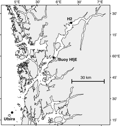
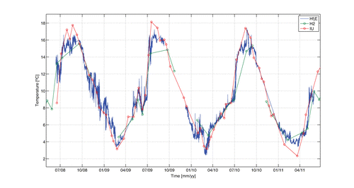
We use observations of temperature from three locations along the main fjord: Utsira, HfjE and H2 (Figure 1). Measurements were taken from 10 m depth with either a CTD-sonde (SAIV SD204, http://www.saivas.no) at section H2 and at Utsira or with a sensor for conductivity number 3919 from Aanderaa Instruments (http://www.aadi.no; accessed 27 Sept 2013) attached to the observational buoy. The technical specifications for the SD204 are: Sampling interval 1 s, resolution of temperature sensor 0.001°C, accuracy of temperature sensor ± 0.01°C, response time of temperature sensor 0.2 s, resolution of pressure sensor 0.01 dbar, accuracy of pressure sensor ± 0.01% FS (sampling frequency), response time 0.1 s. The technical specifications for the conductivity sensor 3019 are: Sampling interval 2 s, resolution of temperature sensor 0.01°C, accuracy of temperature sensor ± 0.1°C, response time 0.1 s. Observations from the IMR coastal monitoring station Indre Utsira are made at approximately 10-day intervals (Sætre et al. 2003) and at section H2 approximately monthly. The temperature observations at the observational buoy HfjE occur as 10-min average values.

Figure 1. Map of the Hardangerfjord showing the locations of the CTD observations and the position of the observational buoy HfjE.

Current measurements are made from either a vertical profiler measuring flow in 1-m bins for a range of 30–50 m (the Nortek Aquadopp Z-cell Profiler, http://www.nortek-as.com) or an Aandreaa Instruments Doppler current sensor DCS4100 (http://www.aadi.no) measuring flow close to the sensor attached to an observational buoy. The technical specifications for the DCS 4100 are: sampling interval 1 s, resolution of speed sensor 0.1% FS, accuracy of speed sensor ± 0.015 m s⁻¹, resolution of direction sensor 0.35°, accuracy of direction sensor ±5°. The technical specifications for the Nortek Z-cell are: sampling interval 1 s, accuracy of speed sensor 1% of measured value ± 0.005 m s⁻¹, accuracy of direction sensor 2°, resolution of direction sensor 0.1°. The current observations at the observational buoy HfjE and the Nortek Z-cell both occur as 10-min average values.

Numerical models

A numerical fjord model simulating current, salinity and temperature has a lot in common with weather prediction models as both solve more or less the same hydrodynamic equations and are of similar complexity. For both weather and ocean predictions, good results rely on a high-quality initial state and most importantly on realistic external forcings. Thus, much effort has been spent in producing high-quality forcings, and we have established a system including several models to be able to simulate current, salinity and temperature and subsequently the spreading of the salmon lice.

The coastal ocean model and the fjord model we use are based on the Regional Ocean Model System (ROMS, www.myroms.org; Shchepetkin & McWilliams 2005; Haidvogel et al. 2008). This is a state-of-the-art, three-dimensional, free-surface, primitive equation numerical model using a generalized terrain-following s-coordinate in the vertical. The s-coordinate levels are adjusted according to the total water depth between the free surface and the bottom, keeping the same number of vertical coordinates for each horizontal grid cell. The advantage of this is that we can maintain a high vertical resolution (< 1 m) at the surface no matter what the sea surface tidal range is. The disadvantage is a potential internal pressure error in the vicinity of steep bottom gradients (Berntsen 2011). The coastal model uses a horizontal grid resolution of 800 m×800 m and is denoted the NorKyst800 model system (Albretsen et al. 2011). The fjord model has a horizontal grid resolution of 200 m×200 m and receives open boundary values from NorKyst800 in a one-way nesting of hourly intervals. Fresh water input from about 100 rivers was put into the model using results of daily runoff from a data-driven hydrological model developed by the Norwegian Water Resources and Energy Directorate (NVE) (Petterson 2008). Results from the 200 m fjord model are stored hourly on the original three-dimensional grid to drive the salmon lice growth and dispersion model.

Atmospheric forcing of the fjord model is important, and the winds are highly influenced by the mountains in the coastal regions of western Norway. Thus, we simulate high-resolution atmospheric fields with the WRF meso-scale wind model (www.wrf-model.org; Dudhia 1993). Results of wind speed and various radiation parameters on a 1 km horizontal grid are fed into the fjord model every 3 h.

The salmon lice growth and advection model is a modified version of a Lagrangian Advection and DIffusion Model (LADIM), which has been used at the IMR for about 20 years (Ådlandsvik & Sundby 1994). Internationally the use of dispersion models for salmon lice has increased for the last ~10 years and is now in a state where fairly realistic results are obtained (Asplin et al. 2004, 2011; Gillibrand & Willis 2007; Amundrud & Murray 2009; Johnsen 2011; Stucchi et al. 2011).

The salmon lice model applies hourly values of simulated currents, salinity and temperature from the fjord model that are interpolated linearly to a subgrid position. The temporal resolution was set to 180 s to make a valid interpolation based on the fjord model's resolution and velocities. The salmon lice model simulates particles swimming up during daytime and down during night, to resemble behaviour found in experiments (Heuch 1995). The first three pelagic larval stages of the salmon louse are simulated, and the duration of the first two nauplii stages are estimated to be 50 degree days and the infectious copepodid stage is estimated to be between 50 and 150 degree days (Asplin et al. 2011). A degree day is a temperature-dependent development time, simply being the product between water temperature and time. For instance 50 degree days apply to both 5 days of constant temperature 10°C and 10 days of constant water temperature 5°C. Output from the salmon lice model with information on the particle position, age, temperature and salinity were given every hour.

Results

Currents and water exchange

The currents in a large fjord such as the Hardangerfjord experience a multitude of forcing mechanisms and hence vary greatly in both time and space. Some parts of the fjord will differ in characteristic current patterns from other parts, e.g. dynamic properties in small and narrow fjord arms versus the wider main fjord.

We chose to present currents from a location in the main fjord half way between the mouth and the head, assuming this current structure to be representative of the major part of the fjord. The observations, shown in Figure 2, are made with a downward measuring current profiler between 1.5 and 40 m depths at 10-min intervals from the position of the observational buoy HfjE covering the period May–June 2011. Only the along-fjord current component is shown (positive values are up-fjord), and we find large variability both vertically and in time. The time variability of the total current from these observations thus includes the variability of all the underlying forcing. In total the situation is rather complicated, as it will be a combination of high-frequency forcing (e.g. tides) to low-frequency forcing (e.g. internal waves). At 1.5 m depth the current speed ranges between 0.7 m s⁻¹ out of the fjord to about 1 m s⁻¹ into the fjord. The variability of the tide is the most frequent oscillation (with period of the M₂ constituent, 12.42 h), and with modest velocity amplitude (~0.05 m s⁻¹), because the observation is from a wide and deep part of the fjord. The single peaks of strong current with a 1–2 day duration are wind episodes, and the shallow outflows are periods where the brackish layer flow is dominating. The inflow episodes down to 30–40 m depth and not always apparent in the upper 5 m are due to the internal pressure-driven flow.

Figure 2. Time series of along-fjord current profiles from 1.5 to 40 m depths at the position HfjE from May and June 2011 as observed with the Nortek Aquadopp profiler. Positive values denote current direction into the fjord.

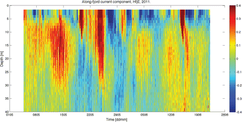
The internal pressure-driven flow typically originates from processes at the coast, changing the vertical stratification of the water masses outside the fjord mouth. Upwelling and downwelling from winds along the coast can cause fluctuations in the internal pressure pattern (Klinck et al. 1981; Asplin et al. 1999; Sundfjord 2010), as can advection of horizontal gradients along the coast (Stigebrandt 2012). The resulting current pattern associated with the internal pressure differences (manifested by plane internal waves) can be long-lasting and have an extension covering the entire fjord to its head. We see from the current observations that the inflow episode lasts between 5 and 10 days with current velocity between 0.1 and 0.3 m s⁻¹ (Figure 2).

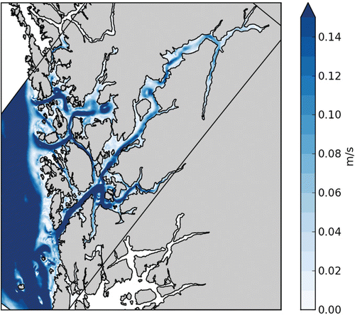
Numerical model results of current speed at 5 m depth from 7 June 2007 are used to illustrate the horizontal extension of such an episode (Figure 3). The flow is into the fjord and extends all the way from the mouth to the head. It does not cover the whole fjord width, but flows in a ~2 km wide stream. At fjord crossings and bends the flow deviates, creating eddies indicating rotational controlled dynamics. The current speed is reduced towards the fjord head.

Figure 3. Current speed at 5 m depth from 7 June 2007, calculated by the numerical model.

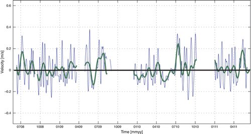
At the position of the observational buoy HfjE we have measured the current at a depth of 10 m from the summer of 2008 for ~3 years. By calculating weekly and monthly mean along-fjord current components, we highlight the most important water exchange components (Figure 4). These mean values will mainly consist of the internal pressure-driven flow. We found 25 weekly mean inflow episodes (positive values) with magnitude above 0.2 m s⁻¹ for this 3-year period, and 39 inflow episodes with a mean velocity above 0.1 m s⁻¹. For the outflow (negative values) there are 6 episodes with a magnitude larger than 0.2 m s⁻¹, while there are 36 outflow episodes with a magnitude larger than 0.1 m s⁻¹. The strongest inflow episodes are observed during the summer, while the strongest outflow episodes are seen during the fall and early winter.

Figure 4. Time series of weekly and monthly (thick line) mean along-fjord current at 10 m depth from the buoy HfjE between the summers of 2008 and 2011. Positive values denote current direction into the fjord.

The consequence of these regular water exchange episodes will be a homogenization of the upper ~50 m of the fjord by mixing coastal water. From temperature observations at the coast and inside the fjord we find that this is the case, as the temperature inside the Hardangerfjord regularly becomes equalized with the values at the coastal station Utsira (Figure 5). Between the episodes of water exchange the temperature inside the fjord can deviate by 1–2 °C due to local processes (as e.g. mixing of discharged freshwater or variable radiation/cloud cover).

Figure 5. Time series of temperature at 10 m depth from observations at the buoy HfjE, at Section H2 and at Indre Utsira (IU) between June 2008 and June 2011.

Salmon lice dispersion

As seen from the fluctuating and generally complex current field in the upper 10–20 m of the Hardangerfjord, the dispersion of planktonic salmon lice will also be highly variable, since they mainly drift with the current. The vertical current shear is occasionally large in the upper ~20 m (Figure 2), and this will effectively spread the individual lice that have the ability to swim upwards or downwards.

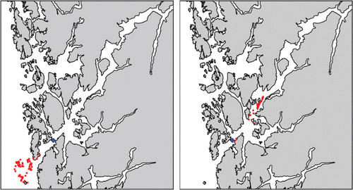
We released 100 lice at a position in the outer part of the Hardangerfjord on 10 and 18 May 2007. Both simulations lasted for 48 h. The lice released on 10 May moved out of the fjord approximately 25 km while the lice released on 18 May moved approximately 25 km into the fjord (Figure 6). The mean advection speed is 0.15 m s⁻¹ in both cases.

Figure 6. Distribution of 100 planktonic salmon lice (red dots) 48 h after the release (at the blue square) on 10 May 2007 (left panel) and 18 May 2007 (right panel).

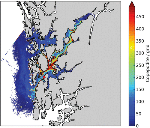
Because salmon lice copepodids obviously can spread in many directions given the many possible current components of the Hardangerfjord, it is generally difficult to determine the dispersion of a single batch of lice larvae from a given source. What we need, however, is knowledge of a potential influence area of salmon lice from a source. Such an influence area must include a sufficient number of possible drift patterns to be representative for a general distribution. How many drift patterns and how long a time period are needed to aggregate a general influence area is not known. As an example, we have run the salmon lice model for 39 days between 2 May and 9 June 2007 with an hourly release of 100 lice. Altogether we will collect the distribution patterns of more than 900 batches of salmon lice for this experiment. This will give an indication of a potential distribution field.

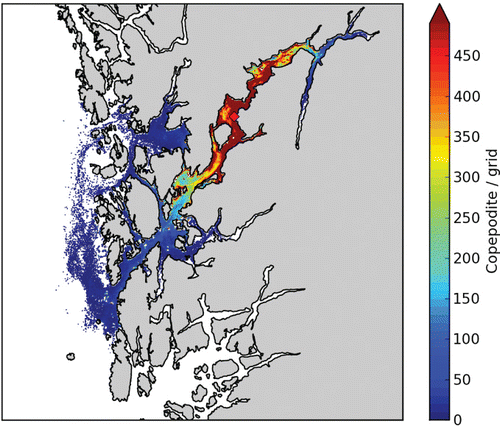
From a release position in the outer part of the main fjord, we expect large variability along the fjord axis (Figure 7). The quantity is copepodids (i.e. only stage 3 of the life cycle of the louse) / m³, but this is somewhat arbitrary as it is an aggregated number for a specific time and number of lice released. The relative spatial differences are realistic, though, and we notice that a small number of lice (blue colour, Figure 7) are widely spread. Areas of higher louse concentrations, however, are much smaller (e.g. red colour). We find these areas with the highest abundance a few kilometres away from the source because we have omitted the two first stages of the lice (~5 days). The lice also tend to accumulate in areas close to shore and in narrows and bays as also found from field observations in Scotland (Penston et al. 2004).

Figure 7. Aggregated density of salmon lice copepodids from a source in the outer part of the Hardangerfjord (red diamond) for the period 2 May to 9 June 2007.

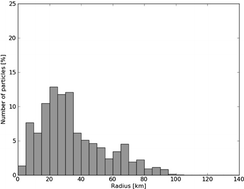
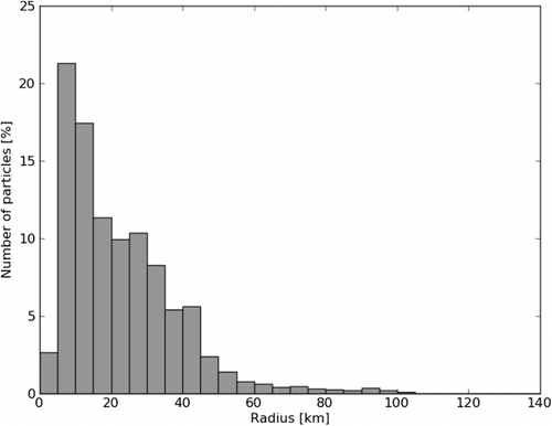
The actual distance from the source for all the salmon lice copepodids shows that most copepodids are gathered 20–40 km away, and only a few travel up to 100 km (Figure 8).

Figure 8. Final spreading of salmon lice copepodids from a source in the outer part of the Hardangerfjord for the period 2 May to 9 June 2007.

If we use a release position further into the fjord, a slightly more enclosed area, we find that the total distribution is less and that the area with higher concentration is larger and centred around the source (Figure 9). The majority of the copepodids travel less than 40 km from their origin, and only a few can travel up to 100 km (Figure 10).

Figure 9. Aggregated density of salmon lice copepodids from a source in the inner part of the Hardangerfjord (red diamond) for the period 2 May to 9 June 2007.

Figure 10. Final spreading of salmon lice copepodids from a source in the inner part of the Hardangerfjord for the period 2 May to 9 June 2007.

Discussion

We find that the most important mechanism for water exchange in the upper ~50 m of a fjord is the current component from internal pressure forces. The pressure at a depth is approximately equal to the weight of the water column above, and any local alteration of the water column stratification will alter the weight and potentially initiate a horizontal pressure force. Typically changes in the water column stratification will occur along the coast outside the Hardangerfjord, either from wind-driven coastal upwelling or downwelling or from internal waves propagating along the coast. Also, the water stratification inside the fjord will be modified either by vertical mixing of the brackish layer or local upwelling or downwelling. Horizontal density differences between the fjord and the coastal water create currents in and out of the Hardangerfjord, and we find that these internal pressure-driven current components are long-lasting and relatively deep (Figure 2). The vertical extension of the current will depend on the stratification and the forcing mechanisms that are responsible for the change of water column stratification. A strong and prevailing wind will, for instance, be necessary for a deep current and possibly fjord basin water renewal. With internal pressure driven current episodes lasting for at least a week, and an associated current system covering the entire length of the fjord with speeds exceeding 0.1 m s⁻¹, water in the upper layer will potentially be transported 150 km, i.e. all the way from the mouth and to the fjord head. This is in accordance with observations of a sudden occurrence of phytoplankton at the fjord head being transported from the coast within a week (Braarud 1975). The current structure will be as plane internal waves, with an opposite current component in the lower layer. In deep fjords, the lower layer of oppositely directed current will be small relative to the upper layer flow (Asplin et al. 1999). In shallower fjords, the lower layer current can be as strong as the upper layer flow (Cianelli et al. 2010).

As the Hardangerfjord is more of a fjord system with many separate fjord arms, the water exchange can differ in various parts of the fjord. Generally the main fjord will have a continuous exchange of water with an approximately monthly interval (Figure 4) for the upper ~50 m (Figure 2). From the three-year time series of current observations at the HfjE buoy, we find the strongest inflow episodes during the summer when the stratification is strongest. The strongest outflow episodes seem to occur in the spring and in the late autumn.

Water exchange and current variability will be of importance for the ecosystem by transportation of nutrients, biota and pathogens. The shorter the life span of an organism is, the more important are the variabilities on shorter time scales. On the other hand, an organism living for longer periods (e.g. macroalgae or mussels) might not be influenced by fluctuations in, for example, the current and temperature within a weekly period. There might be waterborne pathogens living for only a few hours, and then even the tidal driven flow will be important in determining its transportation. Pelagic salmon lice live for 2–4 weeks, and the transport from wind-driven flow and the internal pressure-driven flow will be most important for their distribution. Within its life it might experience several different current regimes, including wind episodes and exchange processes from internal pressure-driven flow. However, during a 2–3 week drift period it might also be relatively calm without strong currents. Also, fluctuations and rapid changes in temperature and salinity might affect the short-living organisms. We find temperature changes of 1–2°C in a short period of time to be relatively frequent (Figure 5). However, the largest variations in salinity and temperature in the Hardangerfjord will be along the vertical axis in the upper 10–20 m, leaving an open question of how a temporal temperature fluctuation at a certain depth will influence an organism that might experience a larger temperature difference by simply moving up or down a few metres in the water column.

Salmon lice copepodids are mainly a threat to wild salmonids, and the major sources for salmon lice are the fish farms (Heuch & Mo 2001). Exactly how the aquaculture industry influences the wild fish populations is not clear, but in order to assess this we need to be able to quantify the abundance of salmon lice copepodids in the fjord system. As seen from the results of the salmon lice dispersion model, we can simulate both episodic distribution of salmon lice batches as well as aggregated salmon lice copepodid distributions (Figures 6–10). The big remaining question is how the abundance of copepodids in a fjord (the dose) actually affects the wild fish population (the response). We lack knowledge on both individual response to salmon lice infection as well as the accumulated response in the population. This is further complicated by the fact that the wild fish populations are influenced by a number of other threats in addition to salmon lice.

If only a small concentration of salmon lice copepodids in the water masses are sufficient to constitute a harmful infectious dose to the wild fish, as illustrated by the widely spread blue colour in Figures 7 and 9, the only possible way of reducing the threat is to ensure that the numbers of salmon lice on the farmed fish are low (by use of medication or cleaner fish) or simply by reducing the total farmed fish biomass in the region. On the other hand, if there is a lower threshold for a necessary dose for infection, as illustrated by the yellow–red colour in Figures 7 and 9, these areas are reduced in extension and it might be possible to reduce the salmon lice threat to the wild fish by relocating fish farms.

Editorial responsibility: Geir Ottersen

Acknowledgements

We are grateful for the support from the crew of RV ‘Hans Brattstrøm’. We have also had invaluable technical assistance from Øivind Østensen and Ole M. Gjervik.

References

- Ådlandsvik B, Sundby S. 1994. Modelling the transport of cod larvae from the Lofoten area. ICES Marine Science Symposia 198:379–92.
- Albretsen J, Sperrevik AK, Staalstrøm A, Sandvik AD, Vikebø F, Asplin L. 2011. NorKyst-800 report no. 1: User manual and technical descriptions. Fisken og Havet, Institute of Marine Reserch 2/2011. 51 pages.
- Amundrud TL, Murray AG. 2009. Modelling sea lice dispersion under varying environmental forcings in a Scottish sea loch. Journal of Fish Diseases 32:27–44. 10.1111/j.1365-2761.2008.00980.x
- Asplin L, Salvanes AGV, Kristoffersen JB. 1999. Non-local wind-driven fjord-coast advection and its potential effect on plankton and fish recruitment. Fisheries Oceanography 8:255–63. 10.1046/j.1365-2419.1999.00109.x
- Asplin L, Boxaspen KK, Sandvik AD. 2004. Modelled distribution of sea lice in a Norwegian fjord. ICES CM 2004/P:11. 12 pages.
- Asplin L, Boxaspen KK, Sandvik AD. 2011. Modeling the distribution and abundance of planktonic larval stages of Lepeophtheirus salmonis in Norway. In: Jones SRM, Beamish RJ, editors. Salmon Lice: An Integrated Approach to Understanding Parasite Abundance and Distribution. Hoboken, NJ: Wiley-Blackwell, p 31–50.
- Berntsen J. 2011. A perfectly balanced method for estimating the internal pressure gradients in σ-coordinate ocean models. Ocean Modelling 38:85–95. 10.1016/j.ocemod.2011.02.006
- Braarud T. 1975. The natural history of the Hardangerfjord. 12. The late summer water exchange in 1956. Its effect upon phytoplankton and phosphate distrubution, and the introduction of an offshore population into the fjord in June, 1956. Sarsia 58:9–30.
- Ciannelli L, Knutsen H, Olsen EM, Espeland SH, Asplin L, Jelmert A, et al. 2010. Maintenance of small-scale genetic stucture in a marine population in relation to water circulation and egg characteristics. Ecology 91:2918–30. 10.1890/09-1548.1
- Dudhia J. 1993. A nonhydrostatic version of the Penn State-NCAR mesoscale model: validation tests and simulation of an Atlantic cyclone and cold front. Monthly Weather Review 121:1493–513. 10.1175/1520-0493(1993)121<1493:ANVOTP>2.0.CO;2
- Gillibrand PA, Willis KJ. 2007. Dispersal of sea louse larvae from salmon farms: modelling the influence of environmental conditions and larval behaviour. Aquatic Biology 1:63–75. 10.3354/ab00006
- Haidvogel DB, Arango HG, Budgell WP, Cornuelle BD, Curchitser E, Di Lorenzo E, et al. 2008. Ocean forecasting in terrain-following coordinates: Formulation and skill assessment of the Regional Ocean Modeling System. Journal of Computational Physics 227:3595–624. 10.1016/j.jcp.2007.06.016
- Heuch PA. 1995. Experimental evidence for aggregation of salmon louse copepodids (Lepeophtheirus salmonis) in step salinity gradients. Journal of the Marine Biological Association of the United Kingdom 75:927–39. 10.1017/S002531540003825X
- Heuch PA, Mo TA. 2001. A model of salmon louse production in Norway: Effects of increasing salmon production and public management measures. Diseases of Aquatic Organisms 45:145–52. 10.3354/dao045145
- Heuch PA, Bjorn PA, Finstad B, Holst JC, Asplin L, Nilsen F. 2005. A review of the Norwegian ‘National Action Plan Against Salmon Lice on Salmonids’: The effect on wild salmonids. Aquaculture 246:79–92. 10.1016/j.aquaculture.2004.12.027
- Klinck JK, O'Brien JJ, Svendsen H. 1981. A simple model of fjord and coastal circulation interaction. Journal of Physical Oceanography 11:1612–26. 10.1175/1520-0485(1981)011<1612:ASMOFA>2.0.CO;2
- Johnsen IA. 2011. Dispersion and Abundance of Salmon Lice (Lepeophtheirus salmonis) in a Norwegian Fjord System. Master's Thesis. Geophysical Institute, University of Bergen. 71 pages.
- Johnson SC, Albright LJ. 1991a. The developmental stages of Lepeophtheirus salmonis (Krøyer, 1837) (Copepoda: Caligoida). Canadian Journal of Zoology 69:929–50. 10.1139/z91-138
- Johnson SC, Albright LJ. 1991b. Development, growth, and survival of Lepeophtheirus salmonis (Copepoda: Caligidae) under laboratory conditions. Journal of the Marine Biological Association of the United Kingdom 71:425–36. 10.1017/S0025315400051687
- Jones SRM, Beamish RJ, editors. 2011. Salmon Lice: An Integrated Approach to Understanding Parasite Abundance and Distribution. Hoboken, NJ: Wiley-Blackwell. 344 pages.
- Penston MJ, McKibben MA, Hay DW, Gillibrand PA. 2004. Observation on open-water densities of sea lice larvae in Loch Shieldaig, Western Scotland. Aquaculture Research 35:793–805. 10.1111/j.1365-2109.2004.01102.x
- Petterson LE. 2008. Beregning av totalavløp til Hardangerfjorden. Norges vassdrags og energidirektorat, oppdragsrapport A nr 9, 2008. 27 pages. ( in Norwegian)
- Shchepetkin AF, McWilliams JC. 2005. The Regional Ocean Modeling System (ROMS): A split-explicit, free-surface, topography following coordinate oceanic model. Ocean Modelling 9:347–404. 10.1016/j.ocemod.2004.08.002
- Stien A, Bjørn PA, Heuch PA, Elston DA. 2005. Population dynamics of salmon lice Lepeophtheirus salmonis on Atlantic salmon and sea trout. Marine Ecology Progress Series 290:263–75. 10.3354/meps290263
- Stigebrandt A. 2012. Hydrodynamics and circulation of fjords. In: Bengtsson L, Herschy RW, Fairbridge RW, editors. Encyclopedia of Lakes and Reservoirs. Berlin: Springer, p 327–44. 10.1007/978-1-4020-4410-6.
- Stucchi DJ, Guo M, Foreman MGG, Czajko P, Galbraith M, Mackas DL, et al. 2011. Modelling sea lice production and concentrations in the Broughton Archipelago, British Columbia. In: Jones SRM, Beamish RJ, editors. Salmon Lice: An Integrated Approach to Understanding Parasite Abundance and Distribution. Hoboken, NJ: Wiley-Blackwell, p 117–50.
- Sundfjord VN. 2010. Volume Transport due to Coastal Wind-driven Internal Pulses in the Hardangerfjord. Master's Thesis. Department of Geosciences MetOs section, University of Oslo. 62 pages.
- Sætre R, Aure J, Danielssen DS. 2003. Long-term hydrographic variability patterns off the Norwegian coast and in the Skagerrak. ICES Marine Science Symposia 219:150–59.