Red sea urchins (Echinus esculentus) and water flow influence epiphytic macroalgae density

Abstract

The importance of forests of the kelp Laminaria hyperborea along the Norwegian coast is related to the three-dimensional structure that they create together with the associated macroalgae. Today, kelp forests have recovered in several areas after an extensive overgrazing by green sea urchins (Strongylocentrotus droebachiensis). However, red sea urchins (Echinus esculentus) have been observed grazing on kelp and algae in recently recovered kelp forests. Apart from grazing pressure, the abundance of algae depends on environmental conditions, such as light and water flow. The main aim of this study was to analyse how densities of red sea urchins, wave exposure and current speed influence densities of epiphytic macroalgae associated with kelp stipes. Our results show that the density of red sea urchins had a negative effect on macroalgal densities. In the well-developed kelp forest (i.e. in a late successional stage found in the southern region), macroalgal density decreased with depth and increased with water flow, both in terms of waves and currents. Wave forces had a higher effect than tidal-driven currents. In the recently recovered kelp forests (in the northern region), we found lower densities of epiphytic macroalgae in shallow compared to deep waters, most likely caused by red sea urchin grazing. Our study concludes that water flow is important for the ecological function of the kelp forest through the influence on habitat-forming epiphytic macroalgae, and that grazing by red sea urchins might severely affect kelp forest resilience in recently recovered areas.

Key words:

• Echinus esculentus
• Laminaria hyperborea
• macroalgae
• sea urchin grazing
• water flow

Introduction

Kelp forests, epiphytic algae and sea urchin grazing

Kelp forests dominate the rocky seabed in the temperate parts of the world and are highly diverse and productive systems (Mann 2000; Smale et al. 2013). The kelp Laminaria hyperborea (Gunnerus) Foslie is widely distributed in the northeast Atlantic, from Portugal in the south (Kain 1971a) to the Murman coast in the north (Schoschina 1997). In Norway, this species dominates the shallow subtidal (< 30 m) and rocky seabed in exposed and moderately wave-exposed areas (Kain 1971a, 1971b; Bekkby et al. 2009). It forms dense forests with rich associated communities of algae and invertebrates with fish, sea birds and mammals using kelp forests as feeding grounds (Whittick 1983; Roen & Bjørge 1995; Bustnes et al. 1997; Norderhaug et al. 2002). A key function of the kelp forests is the three-dimensional structure that the kelp plant, including the holdfast, creates together with the algae growing on the stipes (Christie et al. 2003). The stipe associated epiphytic macroalgae are habitats to a community of mobile animals, with densities reaching several hundred thousand per square metre (Christie et al. 2003). The faunal diversity is regulated by the structural variety of the epiphytic macroalgae (Christie et al. 2007; Norderhaug et al. 2012), and the faunal abundance depends on the total amount and the morphology of the algae (Norderhaug & Christie 2007; Norderhaug et al. 2014).

Overgrazing of macroalgae by sea urchins has been observed worldwide (Harrold & Pearse 1987; Scheibling & Hennigar 1997; Estes et al. 1998). An extensive and long-lasting event (40 years) has dominated large parts of the Norwegian and Russian coast, with green sea urchins, Strongylocentrotus droebachiensis (O.F. Müller, 1776), grazing down the kelp forests in large areas (Norderhaug & Christie 2009). Today, sea urchins have retreated and the kelp forests have recovered in the southern region of the grazed area (e.g. Sjøtun et al. 2001; Fagerli et al. 2013). Green urchins generally avoid the pristine kelp forests (Feehan et al. 2012), but red sea urchins, Echinus esculentus Linnaeus, 1758, have been observed grazing on kelp (Jones & Kain 1967; Norderhaug & Christie 2009) and epiphytic algae (observed by the authors in 2011) in recently recovered kelp forests. Under pristine and kelp-dominated conditions, kelp forests are self-sustained and are, together with the associated epiphytic algae, inhabited by predators feeding on sea urchin recruits, such as crabs (Fagerli et al. 2014) and fish (Tuya et al. 2004). However, grazing on epiphytic algae by red sea urchins is expected to reduce kelp forest resilience by removing habitats important for different sea urchin predators. Young kelp forests with small densities of epiphytic algae and associated invertebrates (i.e. early successional state forest, recently recovered after grazing) are expected to be particularly vulnerable to destructive grazing by sea urchins.

The influence of environmental factors

Apart from grazing pressure, the abundance of epiphytic macroalgae varies with environmental conditions. Algal growth decreases with depth due to decreasing light (Marshall 1960), and species composition might change with factors such as temperature and salinity (Husa et al. 2014). Water flow is a key environmental factor for macroalgae growth, abundance and distribution, both directly through the environmental stress of the exposure pressure and indirectly by affecting factors such as light levels (through turbulence, e.g. Wing & Patterson 1993), transport across boundary layers and consequently nutrient uptake (Raven 1981; Wheeler 1988), settlement, recruitment (Vadas et al. 1990) and resource allocation (Raven 1988). Waves and currents have been found to interact and influence size and biomass of Laminaria hyperborea kelp (Bekkby et al. 2014) and its associated species (Norderhaug et al. 2014).

Grazing pressure is also expected to vary with environmental conditions. Sea urchins avoid shallow areas with high water turbulence (Skadsheim et al. 1995) and are dislodged at high water flow (Denny & Gaylord 1996). Consequently, the moderately exposed and sheltered areas along the Norwegian coast have been dominated by sea urchins, while kelp forests have remained in exposed areas (Sivertsen 1982, 1997; Skadsheim et al. 1995).

In order to learn more about the factors determining the ecological function of the kelp forest, we analysed the relative importance of red sea urchins (Echinus esculentus) and water flow on the amount of epiphytic macroalgae in recently recovered L. hyperborea kelp forests. The main question was how the density of epiphytic macroalgae associated with kelp stipes varies with densities of red sea urchins, wave exposure and current speed, while also accounting for the potential influence of depth, terrain curvature, salinity, temperature, kelp forest density and latitudinal differences. The second question was asked in order to understand more about the sea urchins and how the environmental variables affect sea urchin density. The third question was if young kelp forests are more vulnerable to epiphytic grazing by red sea urchins than old ones, answered by sampling across an area where green sea urchin (Strongylocentrotus droebachiensis) populations have recently collapsed and kelp forests have recovered from destructive grazing.

Methods

Study area and sampling design

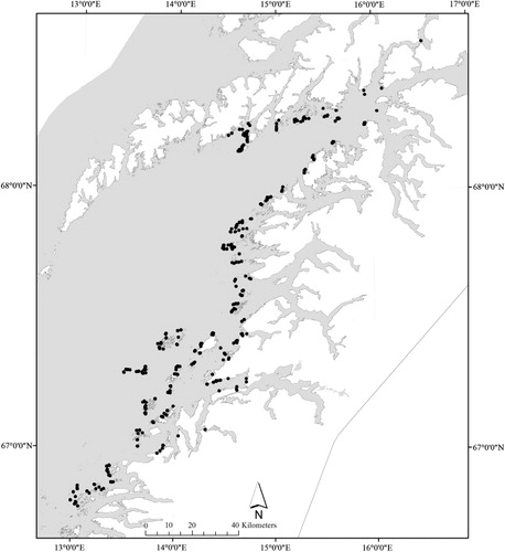
Data were collected from 636 stations with kelp (Laminaria hyperborea) present at different densities in northern Norway (Nordland County), from Salten in the south (southernmost station at 66.8°N) to the Lofoten area in the north (northernmost station at 68.6°N, Figure 1). The study area is formed by inlets, bays, straits, small islands, underwater shallows and rocks. The area receives heavy waves and ocean swells from the west, and has tidal amplitudes of more than 3 m. The variation in bathymetry and terrain creates relatively large spatial differences in current speed.

Figure 1. Map showing the 636 stations with kelp (Laminaria hyperborea) recorded in northern Norway (Nordland County), from Salten in the south (southernmost station at 66.8°N) to the Lofoten area in the north (northernmost station at 68.6°N).

The data were collected in two periods, 30 August–8 September 2011 and 14–29 August 2012, as the density of epiphytic algae is greatest during this time of year (Whittick 1983). GIS models of environmental conditions were used to identify potential sampling stations classified from the range and combinations of environmental conditions within the area. Stations were then selected randomly from this pool of potential stations and georeferenced using a GPS (GARMIN, GPSmap 76Cx, accuracy ± 5 m).

Epiphytic macroalgae and red sea urchins

Kelp (Laminaria hyperborea), epiphytic macroalgae and red sea urchin (Echinus esculentus) densities were identified in the field using an underwater video camera (a ‘drop camera’, Tronitech UVC 5080S, VGA picture resolution 640 × 480) and classified according to the routine established in the Norwegian National Program for Mapping Biodiversity – Coast. Kelp forest density was classified into one of the following four classes: 1 (single individuals), 2 (scarce, i.e. a few individuals), 3 (common/moderately dense, i.e. many plants, but not a completely dense canopy cover), or 4 (dominating, i.e. a completely dense canopy cover). The density of the epiphytic macroalgae growing on the stipe was classified accordingly: 0 (absent), 1 (single individuals), 2 (scarce, i.e. a few individuals), 3 (common/moderately dense, ∼50% of the stipe covered), or 4 (dominating, i.e. the stipe completely covered). Red sea urchin density was classified as 0 (absent), 1 (single individuals), 2 (scarce, ∼2–3 ind.), 3 (common/moderately dense, ∼4–6 ind.), or 4 (dominating, ∼6–8 ind.). The epiphytic macroalgae included in this study were those that were visible using the underwater video camera in the field. Consequently, smaller species/specimens were not included.

Environmental predictor variables

Depth was recorded in the field using the sensor of the underwater video camera. Depth values were standardized relative to the lowest astronomical tide (LAT), which is the standard for ocean data. All other predictor variables were modelled: wave exposure at a 25 m spatial resolution, current speed, salinity and temperature at a 200 m spatial resolution. Table I shows the mean, standard deviation, maximum and minimum values for the environmental variables.

Table I. Mean, standard deviation (SD), minimum and maximum values for the environmental variables used as predictors in the analyses.

Predictors	Mean	SD	Minimum	Maximum
Depth (m)	11.8	7.3	−0.03	37.6
Terrain curvature, 250 m calculation window (m)	3.5	6.9	−25.8	25.3
Terrain curvature, 500 m calculation window (m)	9.5	13.1	−53.6	54.5
Terrain curvature, 1 km calculation window (m)	17.8	21.9	−96.3	94.9
Wave exposure index	371,495	248,007	2488	1,020,289
Mean current speed (m/s)	0.03	0.03	0.00	0.33
Maximum current speed (m/s)	0.28	0.14	0.10	1.50
Mean temperature (°C)	3.38	0.41	2.28	4.88
Maximum temperature (°C)	5.16	0.59	3.93	6.96
Mean salinity (psu)	34.02	0.15	33.51	34.41
Maximum salinity (psu)	34.26	0.14	33.80	34.57

Wave exposure was modelled as an index using data on fetch (distance to nearest shore, island or coast), wind speed and wind frequency (estimated as the amount of time that the wind came from a specific direction, more details in Isæus 2004). Data on wind speed and direction were delivered by the Norwegian Meteorological Institute and averaged over 5 years. The model has been applied in several projects in Norway (e.g. Norderhaug et al. 2012; Pedersen et al. 2012), Sweden (e.g. Eriksson et al. 2004), Finland (Isæus & Rygg 2005), the Danish region of the Skagerrak coast and the Russian, Latvian, Estonian, Lithuanian and German territories of the Baltic Sea (Wijkmark & Isæus 2010).

Current speed (m/s), salinity (psu) and temperature (°C) were estimated as mean and maximum values for the seabed using the three-dimensional numerical ocean model ROMS (Shchepetkin & McWilliams 2005) in a two-level nesting procedure. Level 1: large-scale ocean currents, atmospheric forcing (wind, temperature, pressure, cloud cover, humidity, precipitation and solar radiation), river flow rates and bathymetry were used to drive an ocean model at an 800 m spatial resolution (NorKyst-800, Albretsen et al. 2011). Level 2: in combination with higher-resolution bathymetry, the fields from the 800 m model were used to drive a series of inner models, resulting in a model of 200 m spatial resolution. ROMS has shown good results when compared with field observations (LaCasce et al. 2007) and has users worldwide. To try to capture smaller-scaled differences in current speed, models on terrain curvature were included, with a spatial resolution of 25 m, based on a digital terrain model developed by the Hydrographic Service. Terrain curvature was estimated as the difference between the depth in a given grid cell and the average within three different calculation windows: 250 m, 500 m and 1 km. Negative values indicate small-scale pits or large-scale basins (depending on the calculation windows); positive values indicate shoals (Bekkby et al. 2009).

Statistical analyses

For the statistical analyses we selected cumulative link models (CLM, Agresti 2013) as the primary method (applied in R version 2.15.2, R Core Team 2012). CLMs (R library: ordinal, Christensen 2012) are similar to what is called ‘ordinal regression models’, ‘continuation ratio models’ and ‘proportional odds models’ (McCullagh 1980) and are comparable to its linear or curved counterparts (e.g. Generalized Linear Models, GLMs), but using categorical response variables (here: density classes) with no assumption of the distance between the classes. We included both mean and maximum values of current speed, salinity and temperature, as well as terrain curvature generated by the three different calculation windows. However, only variables less correlated than 50% were included in the same model (Table II for correlations). Kelp (Laminaria hyperborea) density was included as a variable in the analyses. In order to avoid subjective evaluation of which environmental variables should be transformed in order to achieve normally distributed residuals, all environmental variables were transformed to zero skewness at a 0–1 scale prior to the analyses (cf. Økland et al. 2003).

Table II. Correlation matrix (Pearson's R) for the environmental variables.

	Max. temp	Mean temp	Max. sal	Mean sal	Depth	Latitude	Slope	Curv (250 m)	Curv (500 m)	Curv (1 km)	Wave	Max. curr
Mean temp	0.488
Max. sal	−0.485	0.240
Mean sal	−0.587	0.098	0.897
Depth	−0.073	0.041	0.168	0.199
Latitude	0.364	0.489	0.181	0.161	0.187
Slope	−0.177	−0.081	0.212	0.214	0.089	−0.044
Curv (250 m)	−0.290	−0.041	0.164	0.207	−0.315	−0.102	0.139
Curv (500 m)	−0.452	−0.114	0.248	0.300	−0.253	−0.161	0.187	0.911
Curv (1 km)	−0.579	−0.144	0.353	0.401	−0.178	−0.169	0.155	0.719	0.896
Wave	−0.275	−0.224	0.061	0.200	0.261	−0.305	0.032	−0.038	0.039	0.042
Max. curr	0.025	0.045	0.052	0.018	0.165	−0.015	−0.082	0.066	0.064	0.038	0.182
Mean curr	0.010	−0.056	−0.051	−0.060	0.104	−0.044	−0.127	0.071	0.027	−0.009	0.171	0.663

Temp, temperature; sal, salinity; curv, terrain curvature with 200, 500 and 1 km calculation windows; wave, wave exposure index; curr, current speed.

To assure that the results derived from the most appropriate, but not so common, CLM method did not deviate from those derived by more traditional methods, we also applied linear models (LMs), GLMs and generalized additive models (GAMs) to the data. As the models selected using CLM were the same as those selected using more traditional methods, we will only discuss CLM-derived results further. However, as CLM is a relatively new method in R, a sufficiently informative response curve plotting tool is not available. We therefore used the GAM function for plotting partial response curves, as this method allows for nonlinear relationships, as does the CLM.

We used the R library MuMIn (Barton 2013) as a tool for model selection, where all possible combinations of predictor variables made up the set of candidate models tested. We also tested for possible depth-specific effects along the latitudinal gradient (to account for different effects of depth along the north–south gradient) and the wave exposure gradient (as the wave exposure index is a surface model) by including their interactions in the models. Similarly, the different effects of current speed were tested at different levels of wave exposure by including the wave–current interaction. The Akaike Information Criterion (AICc; Burnham et al. 2011) was used as a model selection criterion, in which the best models are the ones receiving most support from the data (i.e. most variation explained), penalized for the number of explanatory factors (i.e. the principle of parsimony). We present and discuss the best model (i.e. lowest AICc) and the simpler models receiving equally good support from the data (ΔAICc < 4, Burnham et al. 2011).

We tested for spatial autocorrelation, i.e. the potential for a correlation in a response amongst stations being spatially close, using Morans I test (Li et al. 2007).

Results

Of the 636 stations, 88 had individuals of Laminaria hyperborea kelp, 215 had scarce densities, 107 were common/moderately dense and 226 were covered by a dense kelp forest. At 367 stations there were no epiphytic macroalgae on the kelp stipes, 44 stations had individuals only, 117 had scarce densities, 78 were common/moderately dense and 30 were completely dominated by epiphytic macroalgae. At 345 stations there were no red sea urchins (Echinus esculentus), 84 stations had single specimens only, 184 had scarce densities and 23 were common/moderately dense. No stations were dominated (i.e. more than six individuals) by sea urchins.

The density of epiphytic macroalgae was best described by the full model (Table III) consisting of (in decreasing order of significance when included in the same model) wave exposure (z = 6.18, p = 6.54 × 10⁻¹⁰), mean salinity (z = 5.08, p = 3.87 × 10⁻⁰⁷), maximum current speed (z = 4.12, p = 3.72 × 10⁻⁵), the depth–wave interaction (z = −3.38, p = 0.0007), the depth–latitude interaction (z = 2.85, p = 0.0044), red sea urchin density (z = −2.84, p = 0.0045), the current–wave interaction (z = −2.66, p = 0.0078), latitude (z = −2.55, p = 0.0108), terrain curvature (with a 250 m calculation window, z = 2.35, p = 0.0189), mean temperature (z = −1.23, p = 0.2171) and depth (z = 0.47, p = 0.6405). The density of epiphytic macroalgae increased with the density of the kelp forest (z = 11.11, p = 2 × 10⁻¹⁶). The model not including terrain curvature and temperature (Model 3 in Table III) received equally good support from the data (i.e. ΔAICc = 3.9, Burnham et al. 2011).

Table III. Overview of the best models explaining the density of the epiphytic macroalgae on kelp (Laminaria hyperborea) stipes and the density of red sea urchins (Echinus esculentus). We present the models with ΔAICc < 4, i.e. the models receiving equally good support from the data (according to Burnham et al. 2011).

Model		AICc	ΔAICc
Density of epiphytic macroalgae
1	wave + sal + depth × wave + curr + depth × lat + urchin + wave × curr + curv + lat + depth + temp	1091.1	0
2	wave + sal + depth × wave + curr + depth × lat + urchin + wave × curr + curv + lat + depth	1091.2	0.1
3	wave + sal + depth × wave + curr + depth × lat + urchin + wave × curr + lat + depth	1095.1	3.9
Density of sea urchins
1	depth × lat + depth + lat + curv(1km)	1337.4	0
2	depth × lat + depth + lat	1337.4	0.34

Wave, wave exposure index; sal, mean salinity; curr, maximum current speed; lat, latitude; urchin, red sea urchin (Echinus esculentus) density; curv, terrain curvature with 250 m calculation window; temp, mean temperature; curv(1km), terrain curvature with 1 km calculation window, × indicates interactions

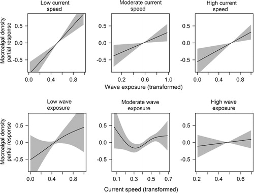
Wave exposure and maximum current speed both positively affected epiphytic macroalgal density, with the effect of wave exposure being stronger and more consistent than that of current speed (Figure 2). Current speed was more important at lower than at moderate or high wave exposure levels (Figure 2), indicated by the interaction between these two variables (Table III). Also, the positive effect of wave exposure decreased with depth. We found a positive effect of terrain curvature (with a 250 m calculation window), and the density of epiphytic macroalgae was higher on shoals than in pits. The density of epiphytic macroalgae increased with mean salinity and decreased with mean temperature.

Figure 2. Partial response curves (with 95% confidence interval) showing the density of epiphytic macroalgae on kelp (Laminaria hyperborea) stipes against wave exposure at low, moderate and high maximum current speed levels (upper panel) and against maximum current speed at low, moderate and high wave exposure index levels (lower panel). Predictor variables were transformed to zero skewness at a 0–1 scale in order to achieve normally distributed residuals.

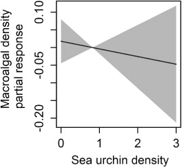
We found a latitude-specific effect of depth and the density of epiphytic macroalgae decreased with increasing depth in the southern region, but increased with depth in the northern region. In the mid region there were no changes in epiphytes with depth (Figure 3, upper panel). Red sea urchin density had a negative effect on the densities of epiphytic macroalgae (Figure 4).

Figure 3. Partial response curves (with 95% confidence interval) showing the density of epiphytic macroalgae on kelp (Laminaria hyperborea) stipes (upper panel) and the density of red sea urchins (Echinus esculentus, lower panel), both plotted against depth in the southern, mid and northern regions of the study area. Predictor variables were transformed to zero skewness at a 0–1 scale in order to achieve normally distributed residuals.

Figure 4. Partial response curves (with 95% confidence interval) showing the density of epiphytic macroalgae on kelp (Laminaria hyperborea) stipes against the density of red sea urchins (Echinus esculentus). Density classes are 0: absent, 1: single individuals, 2: scarce (∼2–3 ind.) and 3: common/moderately dense (∼4–6 ind.).

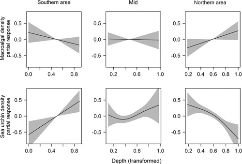
Depth (z = 4.29, p = 1.79 × 10⁻⁵), latitude (z = 2.68, p = 0.007) and the interaction between these two variables (z = −4.48, p = 7.63 × 10⁻⁶) had an effect on sea urchin density (Table III). This was the simplest of the models receiving good support from the data (ΔAICc = 0.34, Burnham et al. 2011). The best model (Table III) also included large-scale terrain curvature (with a 1 km calculation window, z = −2.33, p = 0.02), and the density of red sea urchins was higher on flat terrains and basins than on shoals. The interaction between depth and latitude shows that the effect of depth was not equal along the north–south gradient (Figure 3, lower panel). In the southern and central part of the area there were more sea urchins in the deep areas, while the northern part had more urchins in the shallow areas.

The Moran's I test showed a spatial autocorrelation in the epiphytic macroalgae response of 0.36, with a z score of 8.87. For the red sea urchins, the values were 0.21 and 5.26, respectively. Both z scores indicate a spatial autocorrelation significant at the 5% level.

Discussion

The effect of red sea urchins

Overall, this study found a negative effect of red sea urchin (Echinus esculentus) density on the densities of epiphytic macroalgae. In a fully developed and dense kelp forest, as found in the southern region, the density of epiphytic macroalgae was high. The density decreased with depth, as expected, indicating that the physical conditions (e.g. light and water flow) are the most important factors for the density of epiphytic algae. In these pristine areas, red sea urchins in natural low densities have a minor impact on the epiphytic macroalgae and the ecological function of the kelp forest through the provision of habitats. However, in younger kelp forests in recently recovered areas (i.e. in the northern region), lower densities of epiphytic macroalgae were found in shallow compared to deep waters. This is most likely explained by a high grazing pressure caused by the red sea urchins, as sea urchin densities were higher in shallow than in deep waters.

An explanation for our findings may be that food is highly available to the red sea urchins in pristine, old and dense kelp forests, and that red sea urchin populations are not food-limited, whereas grazing of epiphytic macroalgae in young (i.e. recently recovered) kelp forests may be a more limited resource to red sea urchins. If food supplies are insufficient, red sea urchins might at some point be forced to switch to grazing kelp, which may explain observations of red sea urchins grazing on kelp in recently recovered kelp forests (Jones & Kain 1967; Norderhaug & Christie 2009 and references therein).

Studies have found that sea urchin densities vary with rock type (Scheibling & Raymond 1990). All of our stations were on rocks, but we could not determine whether it was bedrock, boulders or large rocks from field analyses of the underwater video camera. Variation in rock type may have influenced our results, but we do not believe that this has introduced a systematic error in the analyses.

The effect of water flow

The densities of epiphytic macroalgae increased with water flow, both wave exposure and maximum current speed, and we generally found more epiphytic macroalgae at high than at low water flow. The movement of water allows light and nutrients to reach the algae on the stipe through kelp canopy movement induced by the water turbulence. Water movement also makes nutrients more accessible for the algae by increasing the transport across boundary layers (Wheeler 1988; Wing and Patterson 1993). Norderhaug et al. (2014) showed that increased water flow increased habitat diversity, which again increased fauna diversity. This indicates that wave exposure is important for the overall ecological function of the kelp forest. We also found an effect of what most likely are small-scale differences in current speed, indicated by the model on terrain curvature. The density of epiphytic macroalgae was greater on shoals than within pits, most likely indicating a positive effect of water flow. We also found a weak, but significant, effect of large-scale terrain curvature (with a 1 km calculation window) on the density of red sea urchins, with higher sea urchin density in flat terrain and basins than on shoals.

Overall, the wave forces had a higher and more consistent effect than the tidal-driven currents. We observed an interaction between wave exposure and maximum current speed, which shows that the effect of current is not equal at all levels of wave exposures. An increase in current speed had a considerable impact at low wave exposure levels, but was outperformed at high wave exposure levels. This might be due to the high resolution of the wave exposure model (25 m) compared to the current speed model (200 m). However, similar results were also found by other studies applying current speed models of higher resolution (Bekkby et al. 2014; Norderhaug et al. 2014). Consequently, we believe that the results are explained by differences in the mode of the two water forces, wave exposure being more orbital and stochastic and current speed being more regular and bidirectional, possibly allowing more light to enter the stipe-associated algae in the wave-exposed areas and resulting in more kelp canopy shading at high current speeds.

Other significant variables may have reflected different water masses. The observed effect of mean salinity on the density of epiphytic macroalgae is surprising, as all stations were well within the kelp and macroalgae tolerance limit when it comes to salinity. The results most likely reflect different water masses and a fjord–coast–gradient, not the salinity per se. This was also probably the case regarding temperature.

The average distance from one station to the next was 70.9 m (with a standard deviation of 47.7 m), the minimum and maximum distance was 25.2 and 296.3 m, respectively. The Moran's I test revealed that the data in this study were spatially autocorrelated. Spatial autocorrelation is a challenge in species distributions analyses, as it violates the assumption of independence among sample locations. This is quite common in ecological studies, and Diniz et al. (2008) have stated that spatial ecological phenomena produce spatial autocorrelation in biological data, which overestimates the relationships. We did not exclude closely situated stations, as we wanted to make sure that all environmental gradients were covered in an area where these changes occur rapidly within short distances. AIC is considered to provide concise and robust results, and is perhaps the best approach for understanding macroecological patterns (Diniz et al. 2008).

Concluding remarks

Our study indicates that water flow is important for the quantity of epiphytic macroalgae found on kelp (Laminaria hyperborea) stipes, and thereby for the ecological function of the kelp forest. This knowledge is essential for the understanding of ecosystem functioning, and thus deserves attention from managers wanting to protect the biodiversity and preserve ecosystem functioning. It is important to note that our study measured sea urchin densities, not grazing directly. Sea urchin grazing should be verified by analysing sea urchin stomach contents or through stable isotope analyses, neither of which have been possible in this study.

In Norway, red sea urchins (Echinus esculentus) have not been considered a threat to the kelp forests. Our findings, however, strongly indicate that grazing from red sea urchins might have a severe impact on kelp forest resilience in recently recovered areas. The kelp forests and the green sea urchin (Strongylocentrotus droebachiensis) dominated barren grounds are both stable states, because reinforcing mechanisms produce positive feedbacks (Scheffer et al. 2001; Steneck et al. 2004). One important mechanism is the habitat provided for sea urchin predators, securing (‘locking’) the kelp dominance state (Steneck et al. 2013). If the habitat for important predators on newly settled sea urchin recruits is grazed, as indicated by our study (and found by Tuya et al. 2004; Fagerli et al. 2014), the system is pushed towards a tipping point where it more easily flips to the urchin-dominated barren state (Steneck et al. 2013). Recently recovered kelp forests are vulnerable and already close to the tipping point. Thus, while grazing by red sea urchins may have little ecological importance in a late successional kelp forest stage, we predict that it may have a disproportionally high importance in the early stages, in newly recovered kelp forests. Consequently, grazing by red sea urchins should be given high priority by management when considering human activities, including kelp harvesting and fisheries, in areas recently recovered from grazing by green sea urchins. We have no documentation of the effects of fisheries on changing predator pressure on sea urchins in Norwegian waters. However, cascading ecosystem perturbations caused by fisheries have been documented in NW Atlantic coastal waters (e.g. Steneck et al. 2013), and the coastal cod population has declined in Norwegian coastal waters (Kålås et al. 2006). The potential changes in grazing pressure on sea urchins, caused for instance by the northward migration of predators such as the Cancer pagarus crab (Fagerli et al. 2014), should also be considered.

Editorial responsibility: Dan Smale

Acknowledgements

We wish to thank the crew of the University of Nordland ship ‘Tanteyen’ for their field effort and Dag Ø. Hjermann (NIVA) for help with the statistical analyses and plottings.

Additional information

Funding

This project was supported by the Ministry of Climate and Environment and the Ministry of Trade, Industry and Fisheries through the National Program for Mapping of Biodiversity – Coast and by the Norwegian Institute for Water Research (NIVA).

References

- Agresti A. 2013. Categorical Data Analysis. Gainesville, FL: Wiley. 744 pages.
- Albretsen J, Sperrevik AK, Staalstrøm A, Sandvik AD, Vikebø F, Asplin L. 2011. NorKyst-800 Report No. 1: User Manual and Technical Description. Fisken og Havet 2, Bergen. 46 pages.
- Barton K. 2013. MuMIn: Multi-model inference. R package version 1.9.5. http://CRAN.R-project.org/package=MuMIn (accessed 12 October 2014).
- Bekkby T, Rinde E, Erikstad L, Bakkestuen V. 2009. Spatial predictive distribution modelling of the kelp species Laminaria hyperborea. ICES Journal of Marine Science 66:2106–15.10.1093/icesjms/fsp195
- Bekkby T, Rinde E, Gundersen H, Norderhaug KM, Gitmark JK, Christie H. 2014. Length, strength and water flow: Relative importance of wave and current exposure on morphology in kelp Laminaria hyperborea. Marine Ecology Progress Series 506:61–70.
- Burnham KP, Anderson DR, Huyvaert K. 2011. AIC model selection and multimodel inference in behavorial ecology: Some background observations and comparisons. Behavioral Ecology and Sociobiology 65:23–35.10.1007/s00265-010-1029-6
- Bustnes JO, Christie H, Lorentzen SH. 1997. Seabirds, Kelp Beds and Kelp Trawling: A Summary of Knowledge. NINA Impact Assessment Report 472. 43 pages.
- Christensen RHB. 2012. Ordinal – Regression models for ordinal data. R package version 2012.09-11. Computer program. http://www.cran.r-project.org/package=ordinal/ (accessed 2 August 2013).
- Christie H, Jørgensen NM, Norderhaug KM, Waage-Nielsen E. 2003. Species distribution and habitat exploitation of fauna associated with kelp (Laminaria hyperborea) along the Norwegian coast. Journal of the Marine Biological Association of the United Kingdom 83:687–99.10.1017/S0025315403007653h
- Christie H, Jørgensen NM, Norderhaug KM. 2007. Bushy or smooth, high or low: Importance of habitat architecture and vertical position for distribution of fauna on kelp. Journal of Sea Research 58:198–208.10.1016/j.seares.2007.03.006
- Denny MW, Gaylord BP. 1996. Why the urchin lost its spine: Hydrodynamic forces and survivorship in three echinoids. Journal of Experimental Biology 199:717–29.10.4319/lo.1998.43.5.0955
- Diniz JAF, Rangel T, Bini LM. 2008. Model selection and information theory in geographical ecology. Global Ecology and Biogeography 17:479–88.10.1111/j.1466-8238.2008.00395.x
- Eriksson BK, Sandström A, Isæus M, Schreiber H, Karås P. 2004. Effects of boating activities on aquatic vegetation in the Stockholm archipelago, Baltic Sea. Estuarine, Coastal and Shelf Science 61:339–49.10.1016/j.ecss.2004.05.009
- Estes JA, Tinker MT, Williams TM, Doak DF. 1998. Killer whale predation on sea otters linking oceanic and nearshore ecosystems. Science 282:473–76.10.1126/science.282.5388.473
- Fagerli CW, Norderhaug KM, Christie H. 2013. Lack of sea urchin settlement may explain kelp forest recovery in overgrazed areas in Norway. Marine Ecology Progress Series 488:119–32.10.3354/meps10413
- Fagerli CW, Norderhaug KM, Christie H, Pedersen MF, Fredriksen S. 2014. Predators of the destructive sea urchin (Strongylocentrotus droebachiensis) on the Norwegian coast. Marine Ecology Progress Series 502:207–18.10.3354/meps10701
- Feehan C, Scheibling RE, Lauzon-Guay JS. 2012. Aggregative feeding behavior in sea urchins leads to destructive grazing in a Nova Scotian kelp bed. Marine Ecology Progress Series 444:69–83.10.3354/meps09441
- Harrold C, Pearse JS. 1987. The ecological role of echinoderms in kelp forests. Echinoderm Studies 2:137–233.
- Husa V, Steen H, Sjøtun K. 2014. Historical changes in macroalgal communities in Hardangerfjord (Norway). Marine Biology Research 10:226–40.10.1080/17451000.2013.810751
- Isæus M. 2004. Factors Structuring Fucus Communities at Open and Complex Coastlines in the Baltic Sea. Doctoral Thesis. University of Stockholm, Sweden: Department of Botany. 40 pages.
- Isæus M, Rygg B. 2005. Wave Exposure Calculations for the Finnish Coast. Oslo: NIVA Report 5075. 24 pages.
- Jones NS, Kain JM. 1967. Subtidal algal colonization following the removal of Echinus. Helgoländer Wissenschaftliche Meeresuntersuchungen 15:460–66.10.1007/BF01618642
- Kain JM. 1971a. The biology of Laminaria hyperborea VI. Some Norwegian populations. Journal of the Marine Biological Association of the United Kingdom 51:387–408.10.1017/S0025315400031866
- Kain JM. 1971b. Synopsis of Biological Data on Laminaria hyperborea. Rome: FAO Fish Synopsis 87. 74 pages.
- Kålås JA, Viken Å, Bakken T. 2006. Norwegian Red List. Trondheim, Norway: The Norwegian Biodiversity Information Centre. 416 pages.
- LaCasce JH, Røed LP, Bertino L, Ådlandsvik B. 2007. CONMAN Technical Report 2: Analysis of Model Results. Oslo: Norwegian Meteorological Institute Report 5/2007. 44 pages.
- Li H, Calder CA, Cressie N. 2007. Beyond Moran's I: Testing for spatial dependence based on the spatial autoregressive model. Geographical Analysis 39:357–75.10.1111/j.1538-4632.2007.00708.x
- Mann KH. 2000. Ecology of Coastal Waters. Malden, MA: Blackwell. 406 pages.
- Marshall W. 1960. An underwater study of the epiphytes of Laminaria hyperborea (Gunn.) Fosl. British Phycological Bulletin 2:18–19.
- McCullagh P. 1980. Regression-models for ordinal data. Journal of the Royal Statistical Society, Series B 42:109–42.
- Norderhaug KM, Christie H. 2007. Reetablering av tareskog i områder av midt-Norge som tidligere har vært beitet av kråkeboller. Oslo: NIVA Report 5516. 20 pages. ( in Norwegian)
- Norderhaug KM, Christie H. 2009. Sea urchin grazing and kelp re-vegetation in the NE Atlantic. Marine Biology Research 5:515–28.10.1080/17451000902932985
- Norderhaug KM, Christie H, Rinde E. 2002. Colonisation of kelp imitations by epiphyte and holdfast fauna: A study of mobility patterns. Marine Biology 141:965–73.10.1007/s00227-002-0893-7
- Norderhaug KM, Christie H, Andersen GS, Bekkby T. 2012. Does the diversity of kelp forest macrofauna increase with wave exposure? Journal of Sea Research 69:36–42.10.1016/j.seares.2012.01.004
- Norderhaug KM, Christie H, Rinde E, Gundersen H, Bekkby T. 2014. Importance of wave and current exposure to fauna communities in Laminaria hyperborea kelp forest. Marine Ecology Progress Series 502:295–301.10.3354/meps10754
- Økland RH, Rydgren K, Økland T. 2003. Plant species composition of boreal spruce swamp forests: Closed doors and windows of opportunity. Ecology 84:1909–19.10.1890/0012-9658(2003)084[1909:PSCOBS]2.0.CO;2
- Pedersen MF, Nejrup LB, Fredriksen S, Christie H, Norderhaug KM. 2012. Effects of wave exposure on population structure, demography, biomass and productivity of the kelp Laminaria hyperborea. Marine Ecology Progress Series 451:45–60.10.3354/meps09594
- Raven JA. 1981. Nutritional strategies of submerged benthic plants: the acquisition of C, N and P by rhizophytes and haptophytes. New Phytologist 88:1–30.10.1111/j.1469-8137.1981.tb04564.x
- Raven JA. 1988. Algae on the move. Transactions of the Botanical Society of Edinburgh 45:167–86.10.1080/03746608808684958
- R Core Team. 2012. R: A language and environment for statistical computing. Vienna, Austria: R Foundation for Statistical Computing. http://www.R-project.org (accessed 12 October 2014).
- Roen R, Bjørge A. 1995. Haul-out behavior of the Norwegian harbour seal during summer. In: Blix AS, Walløe L, Ulltang Ø, editors. Whales, Seals, Fish and Man. Amsterdam: Elsevier, p 61–68.
- Scheffer M, Carpenter S, Foley JA, Folke C, Walker B. 2001. Catastrophic shifts in ecosystems. Nature 413:591–96.10.1038/35098000
- Scheibling RE, Hennigar AW. 1997. Recurrent outbreaks of disease in sea urchins Strongylocentrotus droebachiensis in Nova Scotia: Evidence for a link with large-scale meteorological and oceanographic events. Marine Ecology Progress Series 152:155–65.10.3354/meps152155
- Scheibling RE, Raymond BG. 1990. Community dynamics on a subtidal cobble bed following mass mortalities of sea urchins. Marine Ecology Progress Series 63:127–45.10.3354/meps063127
- Schoschina EV. 1997. On Laminaria hyperborea (Laminariales, Phaeophyceae) on the Murman coast of the Barents Sea. Sarsia 82:371–73.
- Shchepetkin AF, McWilliams JC. 2005. The regional oceanic modeling system (ROMS): A split-explicit, free-surface, topography-following-coordinate oceanic model. Ocean Modelling 9:347–404.10.1016/j.ocemod.2004.08.002
- Sivertsen K. 1982. Utbredelse og variasjon i kråkebollenes nedbeiting av tareskogen på vestkysten av Norge. Bodø: Nordlandsforskning Report 82. 31 pages. ( in Norwegian)
- Sivertsen K. 1997. Geographical and environmental factors affecting the distribution of kelp beds and barren grounds and changes in biota associated with kelp reduction at sites along the Norwegian coast. Canadian Journal of Fisheries and Aquatic Sciences 54:2872–87.10.1139/f97-186
- Sjøtun K, Christie H, Fosså JH. 2001. Overvaking av kråkebolleførekomstar og gjenvekst av stortare etter prøvetråling i Sør-Trøndelag. Fisken og Havet 5:124. ( in Norwegian)
- Skadsheim A, Christie H, Leinaas HP. 1995. Population reduction of Strongylocentrotus droebachiensis (Echinodermata) in Norway and the distribution of the endoparasite Echinomermella matsi (Nematoda). Marine Ecology Progress Series 119:199–209.10.3354/meps119199
- Smale DA, Burrows MT, Moore PJ, Connor N, Hawkins SJ. 2013. Threats and knowledge gaps for ecosystem services provided by kelp forests: A northeast Atlantic perspective. Ecology and Evolution 3:4016–38.10.1002/ece3.774
- Steneck RS, Vavrinec J, Leland AV. 2004. Accelerating trophic level dysfunction in kelp forest ecosystems of the Western North Atlantic. Ecosystems 7:323–32.10.1007/s10021-004-0240-6
- Steneck RS, Leland A, McNaught D, Vavrinec J. 2013. Ecosystem flips, locks and feedbacks: The lasting effects of fisheries on Maine's kelp forest ecosystem. Bulletin of Marine Science 89:31–55.10.5343/bms.2011.1148
- Tuya F, Boyra A, Sánchez-Jerez P, Barbera C, Haroun RJ. 2004. Relationships between rocky-reef fish assemblages, the sea urchin Diadema antillarum and macroalgae throughout the Canarian Archipelago. Marine Ecology Progress Series 278:157–69.10.3354/meps278157
- Vadas RL, Wright WA, Miller SL. 1990. Recruitment of Ascophyllum nodosum: Wave action as a source of mortality. Marine Ecology Progress Series 61:263–72.10.3354/meps061263
- Wheeler WN. 1988. Algal productivity and hydrodynamics - A synthesis. Progress in Phycological Research 6:23–58.
- Whittick A. 1983. Spatial and temporal distributions of dominant epiphytes on the stipes of Laminaria hyperborea (Gunn.) Fosl. (Phaeophyta: Laminariales) in S.E. Scotland. Journal of Experimental Marine Biology and Ecology 73:1–10.10.1016/0022-0981(83)90002-3
- Wijkmark N, Isæus M. 2010. Wave Exposure Calculations for the Baltic Sea. Stockholm: AquaBiota Report 2. 37 pages.
- Wing SR, Patterson MR. 1993. Effects of wave-induced lightflecks in the intertidal zone on photosynthesis in the macroalgae Postelia palmaeformis and Hedophyllum sessile (Phaeophyceae). Marine Biology 116:519–25.10.1007/BF00350069