High-precision digital light processing (DLP) printing of microstructures for microfluidics applications based on a machine learning approach

ABSTRACT

Digital light processing (DLP) is renowned for its precision, but the challenge lies in the identification of optimal print parameters to minimise print errors and enhance overall print accuracy. This study introduces a groundbreaking approach by integrating 'Random Forest' (RF) models with DLP printing to construct a predictive model for printing errors to achieve unparalleled precision. We conducted experiments using common commercial resins to print, resulting in a comprehensive dataset of 690 experimental datasets. Consequently, we validated this approach by fabricating Y-type microfluidic structures with a minimum feature size printing of 2 µm and herringbone mixer structures with feature sizes of 21.2 µm. We successfully controlled the average print error below 2.3 µm. The 'RF' model was also extended from the printing of microfluidics (2.5D) to complex spatial three-dimensional (3D) Triple-Periodic Minimal Surface (TPMS) structures. We have successfully achieved the printing of TPMS-Gyroid and TPMS-Diamond structures with a minimum feature size of 20 µm, while the printing errors were all kept within 1.5 µm. This study underscores the generalizability and immense potential of integrating machine learning techniques with high-precision DLP printing, offering valuable insights for future research in the realm of high-precision and expeditious 3D printing.

KEYWORDS:

• Digital light processing
• high-precision printing
• printing process optimisation
• machine learning
• microfluidic chip

1. Introduction

Microfluidic and micromachines have drawn significant attention since their introduction in the 1990s [1]. Microfluidics provides precision manipulation of fluids [2,3], biological samples [4], etc., through tiny channels and chambers [5]. They usually have channel dimensions of several tens to hundreds of microns to handle fluids in small quantities from 1 atto-litre to 1 nano-litre [6]. This tiny-scale manipulation allows experiments to be performed on a microscopic scale, where they encompass a tangible enhancement in reaction rates and overall efficiency, resulting in higher precision and sensitivity [7,8].

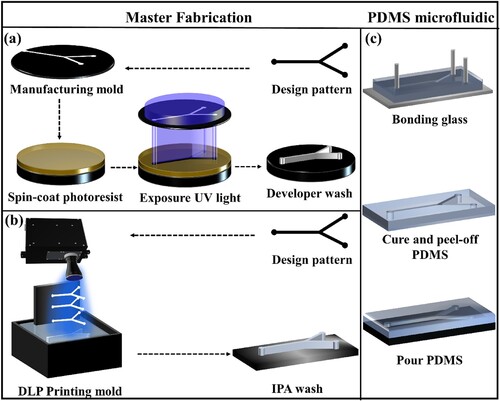
Microfluidic devices were initially fabricated using costly and time-consuming processes like photolithography, etching, and deposition on materials like silicon, quartz, or glass [6,9]. Until the late 1990s, introducing PDMS and soft lithography revolutionised the process, making it significantly more straightforward [10]. Nonetheless, producing PDMS molds through photolithography is still time-consuming and costly, and the exigency for high-precision introduces a heightened level of complexity, thereby amplifying the inherent challenges associated with the rapid development and fabrication of sophisticated microfluidic systems. In recent years, 3D printing has emerged as a next-generation technique for printing complex 3D architectures with micro-scale resolution. As the leading choice for 3D printing in microfluidic mold production, Digital Light Processing (DLP) offers rapid printing, unparalleled accuracy, and superior surface finishes [11–13] compared to traditional microfabrication techniques like lithography [14], wet/dry etching[15] and 3D printing [16]. Figure 1(a) depicts the intricacies of conventional lithography techniques for manufacturing microfluidic chip dies, encompassing pattern design, mask fabrication, glue dumping, lithography, and final cleaning. In contrast, Figure 1(b) showcases the simplicity of the die manufacturing process using DLP, which entails only three manufacturing steps. During the subsequent manufacturing step for generating the PDMS microfluidic chip (Figure 1(b,c)), this streamlined die manufacturing process reduces manufacturing time and enhances flexibility, significantly reduce manufacturing time and increase the success rate and fault tolerance rate of chip production. In 2014, Breadmore et al. [17] presented a pioneering study that employed a commercial DLP printer (Miicraft) to fabricate microfluidic chips with a 250 µm internal diameter. In 2017, MacDonald et al. [18] successfully printed microfluidic devices with a minimum feature size of 94 µm using the Miicraft+ DLP printing system. Building on this progress, Razavi Bazaz et al. [19] in 2020 managed to print microfluidic devices with a width of 200 µm and a height of 50 µm using a DLP 3D printer alongside a newly developed 3D-printing resin while by using the same DLP 3D printer and resin, they printed an 80µm-wide spiral microchip [20]. Notable achievements by Gong, Hua, et al. [21] successfully printed microfluidic chip channels with 18 µm x 20 µm as the smallest microfluidic chip size thus far.

Figure 1. (a) Photolithography steps for mold fabrication. (b) DLP 3D printing steps for mold fabrication. (c) PDMS replica molding for microfluidic devices fabrication.

For DLP printing, how to attain small feature size printing while consistently guaranteeing printing accuracy is still challenge. Especially currently, the minimum features of microfluidic molds is still large than 20 µm. Regrettably, limited research has been devoted to optimising DLP high-precision printing with printing error well controlled. In 2022, Bucciarelli et al. applied the Design of Experiments (DOE) methodology to investigate the influence of printing parameters and used a DLP 3D printer to print pillar structures with 50 µm width [22]. However, the DOE experiments generated a limited amount of data, and the prediction model derived by RSM was limited to quadratic regression equations; thus, the model's predictive capacity remained restricted. In contrast, machine learning offers three notable advantages as an analytical predictive model. Firstly, it can effectively capture non-linear relationships between variables, enabling accurate modelling of complex phenomena [23]. Secondly, unlike traditional statistical models that assume linear relationships, machine learning algorithms can accommodate intricate interactions and dependencies, making them well-suited for diverse applications [24]. Thirdly, machine learning techniques can scale quickly to cope with increasing data, making them versatile for various applications [25]. Machine learning techniques have found successful applications in various domains within the context of DLP printing; researchers have utilised Support Vector Machine (SVM) models to predict the printing speed of Continuous Liquid Interface Production (CLIP) [26], while deep neural network (DNN) models have been employed to explore the intricate correlation between digital input masks and the corresponding output of 3D printed structures, aiming to improve precision and fidelity [27]. Utilising an RNN machine learning model in conjunction with an evolutionary algorithm (EA) to forecast and reverse-engineer the mechanical behaviour of 4D printed active composite beams by DLP. The enhancement of material distribution design, aligned with the properties of the active beam, was realised through the utilisation of an RNN machine learning model [28]. Subsequently, novel methods based on ML and EA were used, and the researchers achieved notable success in swiftly and precisely predicting deformed shapes. This accomplishment has paved the way for the efficient printing of intricate structures [29]. Additionally, The generation of stiffness-modulated scaffolds, characterised by numerous micron-scale features, was realised through the optimisation of printing parameters employing a neural network model-based DLP technology and enabling precise control over the stiffness of the resulting structures [30]. Regrettably, as the critical challenge of DLP technology, limited research has been devoted to optimising DLP high-precision printing parameters. In recent studies, researchers have explored the application of pixel-level grayscale control to enhance printing precision. Notably, they have achieved the printing of circular features as minute as 3.5 pixels. Similarly, these endeavours primarily emphasise the smallest printable features and overlook the comprehensive assessment of the final print error [32]. No study has emerged on combining machine learning models with DLP to achieve high-precision printing with controlled printing error. Addressing conventional DLP printing methods typically relies on trial and error to determine appropriate print parameters, significantly hindering optimising parameters for different printing requirements. Rapid identification of optimal parameters, particularly when using unfamiliar printing systems and untested resins, remains a formidable task. To surmount these challenges, our research endeavours to bridge existing gaps by harnessing machine learning models: Random Forest to attain meticulous 3D printing precision and establish adapt control over printing errors. Our methodology commenced with a thorough analysis of light-curing theory, identifying pivotal printing parameters influencing printing accuracy. Designing, printing, and characterising test structures yielded 690 datasets, each corresponding to distinct print parameters and their associated print errors. These datasets facilitated the training and testing of our ‘RF’ model, culminating in a robust prediction model and optimal print parameters. Our investigation successfully refined printing parameters, yielding microfluidic molds with a minimum feature size of 20 µm for Y-type/herringbone structures (HBS), accompanied by printing errors meticulously constrained within 2.3 µm. Employing these molds for PDMS microfluidic chip fabrication, we observed varying mixing efficiencies of Rhodamine B in ethanol solutions within different structures, validating the efficacy of high-precision mold printing post-parameter optimisation. Expanding the purview of our predictive model to encompass intricate 3D microstructures, specifically Triple-Periodic Minimal Surface (TPMS), we achieved precise printing of TPMS-Gyroid and TPMS-Diamond structures with a minimum feature size of 20 µm while maintaining an overall printing error consistently within 1.5 µm. This extension underscores the pragmatic applicability of our approach. Our study pioneers the optimisation of process parameters, harmonising machine learning models with DLP printing technology for steadfast and high-precision printing of micron-scale structures. Beyond showcasing the potential of DLP technology in microfluidic chip device development and advancing printing technology frontiers, our work provides a compelling solution with broad implications for researchers and practitioners alike.

2. Materials and method

2.1. Materials

In this study, clear resin from Phrozen Technologies Ltd. (Taiwan) was deliberately used as the primary resin based on its wide availability and representation of commercially available resins. The resin formulation consists of Acrylate oligomer, 4-(1-oxo-2-propenyl)-morpholine, Bis(1,2,2,6,6-pentamethyl-4-piperidyl) sebacate, and Diphenyl (2,4,6-trimethyl benzoyl) phosphine oxide (<5%) as its main components. Therefore, the successful printing of high-precision three-dimensional structures using this clear resin in this study not only showcases the capabilities of the printing equipment but also confirms the effectiveness of the optimised printing conditions used in this research. This achievement serves to validate the advanced printing capabilities of the equipment and the validation of the optimised printing conditions. In the fabrication process of PDMS microfluidic chips, a mixture of Sylgard 184 (Dow, Midland, MI, US) and RTV 615 (GE Silicones) was employed at 10:1.

2.2. DLP printing system

A high-resolution DLP 3D printing system has been developed for micro-scale precision additive manufacturing (Figure 2(a)). The system employs a high-precision digital light engine (Wintech Digital Systems Technology Corp. San Marcos, CA, USA) with a printable area of 14.66 mm × 8.25 mm and a horizontal resolution of 5.4 µm. A customised motorised stage is employed to move the printing platform vertically, enabling high-resolution printing in the vertical direction. The stage exhibits a bidirectional repeatability of less than 1 µm and a substantial load capacity of 4 kg. The control system and graphical user interface (GUI) were designed by LabVIEW (National Instruments, Austin, TX, USA) to ensure precise control of the printing process. To improve user-friendliness and minimise direct exposure to photopolymer resin, a CCD camera integrated with a triaxial adjustment mechanism enables remote and real-time monitoring of the printing process and print status.

Figure 2. (a) Customized DLP printing system components. (c) Print schematic. (d) DLP printing flow chart. (e) Test the spectrum of the digital light engine. (f) Measure the UV light power of the digital light engine.

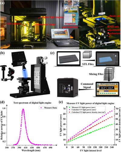
A concise description of the printing mechanism employed by the in-house assembled DLP printing system is shown in Figure 2(c). The system leverages a customised UV pattern with a wavelength of 405 nm, which is projected onto the resin surface inside the resin vat through a digital micromirror device (DMD)-based digital light engine. Subsequently, the Z-axis motorised platform moves down and up a certain distance after a designated curing time, and the curing process is repeated until the end of the printing procedure. As depicted in Figure 2(d), before the DLP printing process, the three-dimensional (3D) structure necessitates using dedicated 3D modelling software and exporting it into STL files. These files are sliced into a sequence of 2D images using professional slicing software before being transmitted to the DLP system. The GUI enables users to set the exposure time, UV light intensity, and print speed. As an essential component of the DLP printing system, the digital light engine requires thorough verification and validation of its optical power. To measure the UV spectrum and determine the relative UV light power of the light source, a spectrometer (OTO 2090 Spectrometer, Taiwan) was employed, revealing a relative light power value of 0.992 at the central wavelength of 405 nm (Figure 2(e)). The output power of the UV light was determined precisely using the Sensor Power Meter PM160 (Thorlabs, Inc., Newton, NJ) (Figure 2(f)). The measured UV light output power ranged from 7.47 to 69.13 mW, depending on the design specifications and (post-)printing requirements.

2.3. Microstructure characterization

3D structures that were produced were subjected to rigorous characterisation to understand their morphology and surface properties for target microfluidic applications. Initially, an optical microscope (Keyence, HX-5000, Japan) was used to determine the printed structures’ 3D profile, height, and width. For a more comprehensive understanding of their morphology, scanning electron microscopy (SEM) was employed. Before SEM imaging, the samples were coated with a 10 nm thick gold layer using sputtering (CCU-010 LV, Safematic GmbH, Switzerland) to enhance conductivity and prevent sample charging. High-resolution SEM images were obtained using a Hitachi SU8020 field-emission scanning electron microscope. This enabled the identification of any defects or irregularities in the printed structures. A Bruker NPFLEX, white light interferometer was used to measure their three-dimensional profiles and determine their roughness characteristics. Analysis of the surface profile data facilitated quantifying the roughness of the printed structures and identifying any features or irregularities resulting from the printing process. Overall, this comprehensive characterisation procedure enabled a more in-depth assessment of the quality and properties of the 3D-printed structures.

2.4. Printing methodologies

2.4.1. Exploring key process parameters for photopolymerization

Jacobs’ model has been employed extensively as a crucial tool to optimise the photopolymerization printing parameters and achieve high-precision printing [33]. In light of the ‘Jacobs working cure,’ the application of irradiation exposure is administered instantaneously for each layer and the corresponding irradiation energy $(\mathit{E})$ that is transmitted to the surface of the photopolymer resin can be mathematically represented as [34]: (1) $E=T{I}_0$(1) By assuming that the resin is positioned at $z=0$, the optical irradiance is represented by $I_0$, and $T$is used to signify the light intensity and exposure time correspondingly. The ‘Working curve model’ developed by Jacobs’ Matrix can be expressed mathematically as: (2) $C_d=D_p\ln \left({\displaystyle \frac{E_{\max }}{E_c}}\right)$(2) Within this context, $C_d$ represents the thickness of the cured resin layer. $E_{\max }$ denotes the maximum energy exposure density, which represents the energy density of a light beam before it enters a pool of photopolymer resin. Jacobs’ principle introduces two key parameters: the penetration depth of the curing time, denoted as $D_p$, and the energy required for polymerisation, designated as $E_c$[35]. The light penetration follows a Beer–Lambert relationship [36, 37]: (3) $P_z=P_0{e}^{-z/D_p}$(3) In this scenario, $P_z$ represents the UV light dosage at the depth $z$, while $P_0$ stands for the initial dose at the surface (z = 0). To achieve superior printing accuracy, it is essential to optimise the values of $D_p$ and $E_c$. This optimisation process requires a considerable amount of experimental data. Specifically, $D_p$ is equivalent to the slope of the ‘working curve,’ whereas $E_c$ of exposure time T corresponds to the intersection point of the straight line of the side measurement data with the X-axis. To achieve the highest printing accuracy, it is essential to consider both the thickness of the cured layer, $C_d$, and the cured width of the microscale structure. In Jacob's model, the cured linewidth is denoted as $L_w$. Equation (4)(4) $L_w={\omega }_0\sqrt{2{\displaystyle \frac{C_d}{D_p}}}$(4) illustrates that the maximum width depends on both the cured resin layer, $C_d$, and the penetration depth of the curing time, $D_p$, highlighting the importance of $C_d$ and $D_p$ in determining the curing width of the resin surface. (4) $L_w={\omega }_0\sqrt{2{\displaystyle \frac{C_d}{D_p}}}$(4) The width of the curing surface exhibits a direct correlation with the projection width radius of the UV light beam $({\omega }_0)$ at the topmost resin surface. Additionally, the cured width displays proportionality to the square root of the ratio $C_d/D_p$, indicating that both the thickness and width of the cured layer are directly affected by $C_d$ and $D_p$. The penetration depth $D_p$ in the photopolymer resin is contingent upon its composition and formulation. Crucially, the ultimate exposure energy is shaped by two pivotal parameters: UV exposure time and UV light intensity, which indirectly governs the curing resin thickness $C_d$ and curing line width $L_w$. Thus, UV light intensity and exposure time directly impact the printing accuracy of the cured microstructure. Furthermore, in DLP printing, the print layer thickness emerges as a pivotal determinant of the longitudinal accuracy of 3D structures. Thinner print layer thickness inherently contributes to enhanced layer-by-layer precision, affording meticulous control over the shape and positioning of each layer. Likewise, the thinner layer thickness facilitates heightened spatial resolution. This attribute becomes particularly crucial when fabricating structures characterised by intricate geometries or minute features. Hence, the print layer thickness, being a critical printing parameter, exerts a direct influence on the ultimate print accuracy. Meticulous adjustment and control of the print layer thickness throughout the DLP printing process stand as imperative steps in realising high-precision printing. Therefore, different UV exposure times, UV light intensity and layer thickness combinations will be used to examine their relationship with the ultimate print accuracy.

2.4.2. Polynomial regression model

Linear regression is a part of the general linear model (GLM) that is often used to predict one variable from another [38]. Simple linear regression can be expanded to include more than one predictor variable to become multiple linear regression (MLR) [39]. Polynomial regression is a special case of multiple regression, with only one independent variable $x$, with the dependent variable $y$ linearly depending on the power of the single independent variable $(x,x_1,x_2,\dots ,x_k)$. A one-variable polynomial regression model with kth order can be expressed as (5) $y={\beta }_0+{\beta }_1{x}_i+{\beta }_2{x}_i^2+{\beta }_3{x}_i^3\dots +{\beta }_k{x}_k^k+e_i,\mathrm{for}i=1,2,\dots ,n$(5) where $y$ is the measured or observed variable at time $x,$ $k$ is the order of the polynomial, and the $\beta$ are the unknown parameters to be estimated. The $e_i$ is the error term, which is also time-dependent and follows the probability distribution of $y$. To get the average absolute difference between the predicted and actual values, the Mean Absolute Error (MAE) assessment metric is used to measure the average absolute difference between the predicted and true values of the target variable. It is calculated as the average of the absolute differences between the predicted and true values, as shown in equation (6): (6) $\mathrm{MAE}={\displaystyle \frac{1}{n}\times \sum |y-y_i^{{}^{\mathrm{\prime }}}|\mathrm{for}i=1,2,\dots ,n}$(6) Here, $n$ is the number of printed structures, y is the true value, and $y_i^{\mathrm{\prime }}$ is the i-th predicted value. The Mean Absolute Error (MAE) is robust to outliers since it computes the absolute value of the differences between predicted and true values. Apart from MAE, another widely used metric to evaluate the performance of regression models is known as $R^2$ (coefficient of determination). $R^2$ indicates a better fit of the model to the data, which ranges from 0 to 1 and demonstrates how well the model fits the data. The value of $R^2$ always falls between zero and one,$0\ll R^2$ $\ll 1$. An $R^2$ value of 0.9 or higher is considered excellent, a value above 0.8 is good, and a value of 0.6 or above may be acceptable in specific applications [40,41]. The $R^2$ of multiple regression is similar to the simple regression where the coefficient of determination $R^2$ is defined as: (7) $R^2=1-{\displaystyle \frac{\mathrm{SSE}}{\mathrm{SST}}=1-{\displaystyle \frac{{\sum }_{i=1}^n{(y_i-{\hat{y}}_i)}^2}{{\sum }_{i=1}^n{(y_i-\overline{y})}^2}}}$(7) As a quintessential predictive approach, polynomial regression models provide enhanced flexibility in capturing intricate data patterns by incorporating polynomial terms to improve the goodness of fit. In addition to their simplicity and computational efficiency, polynomial regression models outperform certain complex models. Their ability to require fewer computational resources allows for expedited training and evaluation processes. Consequently, polynomial regression models are used extensively in diverse scenarios.

2.4.3. Random forest model

‘RF’ is a regression technique that employs a multitude of decision tree (DT) algorithms to classify or predict the value of a variable[41–43]. When presented with an input vector $(x)$ composed of the values of different evidential features evaluated for a given training area, ‘RF’ generates $K$ regression trees and computes the average of their results. Once $K$ trees $\{T(x){\}}_1^K$have been constructed, the ‘RF’ regression predictor can be expressed as: (8) ${\hat{f}}_{\mathrm{rf}}^K(x)={\displaystyle \frac{1}{K}\sum _{k=1}^{K}T(x)}$(8) To avoid the correlation among the different trees, ‘RF’ enhances the diversity of the trees by growing them from different training data subsets generated through a bagging technique. Bagging is a technique used for training data creation by randomly resampling the original dataset with replacement, i.e. by selecting data from the input sample without deleting it to generate the following subset $\{h(x,{\theta }_k,k=1,\dots ,K)\}$, where $\{{\theta }_k\}$. are independent random vectors with the same distribution [45]. Some data may be used more than once in training, while others might never be used. Thus, better stability is achieved, as it makes it more robust when facing slight variations in input data and, at the same time, increases prediction accuracy[42]. Unlike most machine learning methods, ‘RF’ only needs two parameters to be set for generating a prediction model: the number of regression trees and the number of evidential features (m); increasing the number of trees always leads to convergence of the generalisation error, and reducing the number of m reduces the correlation among trees, thereby increasing the model's accuracy, which is used in each node to make regression trees grow [46].

As a robust regression prediction model, ‘RF’, by integrating multiple decision trees, mitigates the risk of overfitting and enhances the overall stability and precision of the model. Notably, the ‘RF’ model exhibits robustness due to missing values and outliers. It effectively handles datasets containing these anomalies and consistently yields reliable predictions. As a result, the ‘RF’ model has emerged as a popular choice in machine learning for prediction tasks, consistently delivering exceptional performance across various practical problems.

2.5. Data collection

2.5.1. Design and printing of test structures

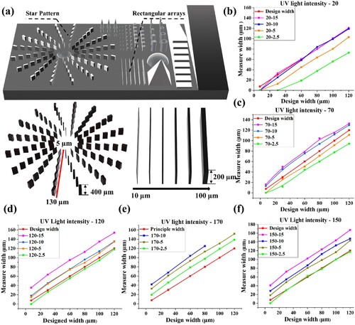
Figure 3(a) illustrates a specialised test structure designed for the comprehensive collection of experimental data under varying UV irradiation times, light intensities and layer thickness. This design aims to acquire substantial experimental data in a single experiment while ensuring optimal printing precision for structures with diverse feature sizes. The test structure comprises two distinct components: the ‘star pattern’ ring structure and the ‘rectangular array structure’. The star pattern is an annular structure with a height of 400 µm, exhibiting a star pattern high aspect ratio that gradually decreases from 80 to 3 as the width expands in 10 µm increments from 5 µm to 130 µm from the inner to outer regions, respectively. The rectangular array structure is also introduced to circumvent potential influences from shape and height variations on final printing accuracy. With a height of 200 µm, it consists of rectangular widths ranging from 100 µm to 1,000 µm in increments of 100 µm from left to right. Notably, the DLP printing system allows for adjustment of the light intensity within the 0–255 range, necessitating the determination of an appropriate UV light intensity based on specific printing requirements. According to the experiment design, selected an appropriate layer thickness of 50 µm as an initial step. Subsequently, leveraging the experimental data obtained at the 50 µm layer thickness, systematically expanded additional parameter ranges with different layer thicknesses. Careful consideration was given to selecting an appropriate range of 50 µm layer thickness, the UV light intensity was set between 20–170. A UV light intensity of 20 (10.25 mW/cm²) was deemed suitable for use in the 3D bioprinting to ensure that cells and other active molecules would not be damaged, while a UV light intensity of up to 170 (41.49 mW/cm²) was considered sufficient for lithography. After determining the UV light intensity, the exposure time was chosen with a decreasing gradient within 15 s (15, 10, 5, 2.5).

Figure 3. (a) Test structure star pattern structure and rectangular array structure with 50 µm layer thickness. (b-f) Different measure widths at different exposure times at UV intensity; (b) UV light intensity 20, (c) UV light intensity 70, (d) UV light intensity 120, (e) UV light intensity 170, (f) UV light intensity 150.

2.5.2. Data acquisition and analysis

The accuracy of DLP 3D printing relies heavily on selecting appropriate UV light intensity, exposure time, and layer thickness, which can be set up from the control system and used to control the process of curing the clear resin. To ensure the fidelity of measurements and eliminate any potential interference from impurities or residues, the printed structures were thoroughly cleansed by rinsing them with isopropyl alcohol (IPA) and left to air dry at room temperature for 24 h. Figure 3(b-e) presents the measured widths of the printed structures under different light intensities and exposure times with 50 µm layer thickness. The red line represents the ideal width of the print structure, and the proximity of the print data to the red line indicates smaller true print errors. Analysis of the printing results at varying light intensities reveals that an increase in exposure energy leads to larger print widths under a specific light intensity. However, as the UV energy further increases, the issue of over-curing becomes more pronounced, resulting in severe deformation and printing failure. As demonstrated in Figure 3(e), at a light intensity of 170 and an exposure time of 15 s, over-curing is evident, leading to unsuccessful printing. Additionally, a comparison of Figure 3(b-e) demonstrates that the overall pattern based on the ideal width (red line) exhibits an upward trend with higher light intensities. For instance, at a light intensity of 20 and an exposure time of 15s, the print width approaches the ideal width (Figure 3(b)), while at a light intensity of 120 and an exposure time of only 2.5s, it already closely approximates the ideal width (Figure 3(d)). These observations not only confirm the accuracy of the measurements but also underscore the scientific validity of the experimental data. To further validate the reliability of the experimental data, a separate experimental group was printed, measured, and characterised as a validation group, as shown in Figure 3(f). Comparing Figure 3(d–f), the print width under a light intensity of 170 with an exposure time of 2.5s closely aligns with the ideal width, while the print width under a light intensity of 120 with an exposure time of 2.5s falls below the ideal width. As shown in Figure 3(f), the print width is close to the ideal under a light intensity of 150 and an exposure time of 2.5s. These findings indicate that the print width at a light intensity of 150 falls between that of a light intensity of 120 and 170. These observations are entirely consistent with the theory of DLP light curing and further validate the experimental data's reliability for subsequent model establishment. Moreover, the experiments also reveal the criticality of selecting appropriate printing parameters for high-precision printing, as different parameters yield distinct printing errors. The UV intensity range was extended from 20 to 170, and UV exposure time was extended from 2.5 to 15s to address localised model optimisation and enable broader data coverage.

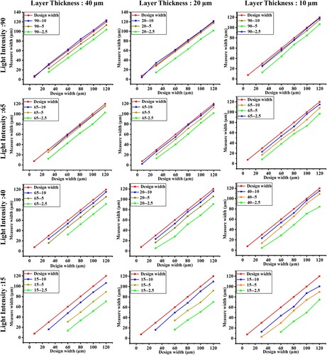
In the realm of the DLP printing process, the conventional theoretical emphasis on UV light intensity and exposure time in the horizontal dimension necessitates nuanced consideration. The thickness of the printed layers emerges as a critical determinant of printing accuracy in the vertical domain, with smaller layer thicknesses correlating positively with smaller surface roughness. To comprehensively address these considerations, distinct layer thicknesses were introduced at 40, 20, and 10 µm to explore the impact on printing outcomes meticulously. Aligned with the 50 µm layer thickness printing parameters range, UV light intensity was judiciously set at 90, 65, 40, and 15, and exposure times at 10s, 5s, and 2.5s, respectively. This strategic calibration facilitated exhaustive coverage of diverse layer thicknesses. Figure 4 encapsulates the salient outcomes of this rigorous experimentation,illustrating the printing results corresponding to distinct exposure times and intensities for layer thicknesses spanning 10–40 µm. Specifically, Figure 4(a,d,g,j), (b,e,g,h), and (c,f,I,l) represent the measured values corresponding to varied UV light intensities and exposure times for layer thicknesses of 40, 20, and 10 µm, respectively. The discernible patterns in Figure 4 underscore the nuanced interplay between diverse printing parameters and layer thicknesses, elucidating the profound influence on resultant printing errors. It also shows that for high-precision printing, once the print material is standardised, the judicious selection of appropriate printing parameters and layer thickness assumes paramount importance in determining final printing accuracy.

Figure 4. (a-c) Different measurement widths for different layer thicknesses and exposure times under UV light intensity 90; (a) 40 µm. (b) 20 µm, (c) 10 µm. (d-f) Different measurement widths for different layer thicknesses and exposure times under UV light intensity 65; (d) 40 µm. (e) 20 µm, (f) 10 µm. (g-i) Different measurement widths for different layer thicknesses and exposure times under UV light intensity 40; (g) 40 µm. (h) 20 µm, (i) 10 µm. (j-l) Different measurement widths for different layer thicknesses and exposure times under UV light intensity 15; (j) 40 µm. (k) 20 µm, (l) 10 µm.

2.5.3. Data distribution and processing

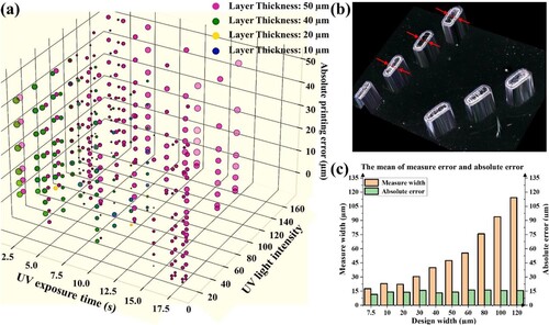
A comprehensive set of 690 data sets constitutes the experimental foundation of this study. In Figure 5(a), the visual representation of actual printing errors under diverse printing layer thicknesses, UV light intensities, and exposure times unveils a balanced and inherently independent distribution with discernible randomness. This equitably distributed dataset serves as a linchpin for conferring robust learning and predictive capabilities to the model across all sample categories. Consequently, the dataset exhibits enhanced generalisation under varied conditions, augmenting the model's precision. Figure 5(b) elucidates the meticulous measurement methodology designed to elevate accuracy and ensure data integrity. A designated ‘centre line’ along the structure serves as the reference point, located at the structure's midpoint and employed as the observation point. Three measurements per structure, coupled with averaging to accommodate potential variations, fortify the reliability and accuracy of our dataset. Within the context of the light-curing printing process, the perils of insufficient curing energy (‘under-curing’) lead to incomplete or uncured structures and excessive curing energy (‘over-curing’) causes anomalous increases in cured structure size necessitate careful consideration. To enhance data authenticity and precision, the experiment dataset excluded measurement outliers and missing values attributed to ‘under-curing’ or ‘overcuring,’ resulting in a refined dataset comprising 555 sets of measurements. This curation step ensures data reliability without compromising the subsequent model's predictive prowess. Following the acquisition of all experimental data, a meticulous analysis was conducted to validate and evaluate the results comprehensively. Figure 5(c) distinctly illustrates a discernable correlation between design dimensions and actual printed dimensions. Noteworthy is the consistent mean absolute error across various sizes, indicating an absence of a direct correlation between print error and design size. Additionally, irrespective of designed size variations during the printing process, the print error remains stable, emphasising its significance and sensitivity for smaller structures. Even marginal print errors can yield substantial relative errors, therefore underscoring the criticality of promptly ascertaining optimal print parameters and effectively managing print errors to attain high accuracy in DLP printing.

Figure 5. (a) Actual distribution of absolute printing errors for different layer thicknesses, UV light intensities, and exposure times, (b) Measurement position of the ‘Mid-centre line’ of cured structure, (c) Mean and average absolute printing errors of the actual prints.

Therefore, selecting appropriate printing parameters is crucial for successful high-precision micro-scale printing. To investigate the intricate relationship between different light intensities, exposure times, and printing errors, a dataset comprising 555 measurements of printed structures was meticulously compiled. These data were subsequently integrated into various machine-learning models to analyse the printing errors and their corresponding printing parameters comprehensively. The overarching objective was to enhance the DLP printing process by applying machine learning models, thereby elevating the precision and accuracy of the printed structures and enabling precise control over printing errors. Table 1 provides a comprehensive overview of the experimental printing parameters, encompassing key quantitative variables. It is important to note that certain process parameters that significantly impact the printed structures, such as UV intensity, exposure time and layer thickness, were deliberately varied. Meanwhile, other process parameters were constant, including ultrasonic cleaning time, and post-processing time. This deliberate approach ensures a focused analysis of specific variables within the study while maintaining strict control and consistency throughout the experimental setup.

Table 1. Design of experiment process parameters.

Factors	Type	Minimum Value	Maximum Value
Light Intensity	Variable	15	170
Exposure Time	Variable	1s	18s
Layer Thickness	Variable	10µm	50µm
Star Pattern Width	Variable	5µm	130µm
Rectangular Array Width	Variable	10µm	100µm
Fixed Factors
Sonication Time	Fixed	10min
Print Temperature	Fixed	25 °C
Sonication Time	Fixed	10min
Post-cured Time	Fixed	10min

2.6. Printing height characterisation analysis and correction

The total height of the vertical dimension in the printed test structure was specified as 2 mm, comprising a substrate thickness of 1.6 mm and a microstructure thickness of 0.4 mm. Following this determination, the test structure underwent printing with varying combinations of parameters, allowing for a comprehensive exploration of their impact on the final printing height. Height characterisation was obtained by optical microscopy scans of the 3D profile, and it was observed that the print height consistently fell within the 340–348 µm for variations in the print parameters. This observation suggests that the structure's height is independent of the print parameters. The layer thickness was primarily influenced by the bi-directional repeatability error of the Z-axis displacement stage and the initial position between the top surface of the resin barrel and the Z-axis printing stage. The custom-designed Z-axis motorised stage demonstrated a bi-directional repeatability error of less than 1 µm, suggesting that the height error was mainly due to the initial position of the resin drum. As a result, the structure was reprinted and scanned in a 3D profile after repositioning the resin barrel. The final height of the structure was 399.5 µm, indicating that the re-tuned DLP printing system demonstrated high print accuracy and positioning accuracy in terms of print height for high-precision 3D printing.

3. Results and discussions

3.1. Printing width error prediction

Upon careful examination of the collected data, as shown in Figure 5(a), it becomes apparent that the relationship between UV light intensity, UV exposure time, layer thickness and the resulting printing error does not exhibit a straightforward linear pattern. This study aims to establish a prediction model capable of estimating printing errors based on different printing parameters. It is crucial for this model to possess the requisite flexibility to enhance prediction accuracy across various model parameters. Machine learning models offer notable advantages, particularly their ability to automatically learn and capture intricate relational patterns, facilitating more precise predictions and interpretations. After considering the predictive ability, interpretability, computational efficiency, and implementation complexity of different models, this paper selects two fundamental machine learning models, ‘RF’ and Polynomial regression, as predictive models. Polynomial regression, a classical statistical model, enjoys extensive usage in predicting and elucidating variable relationships. Conversely, the ‘RF’ is a potent non-linear predictive model adept at handling intricate relationships and interactions. This model exhibits adaptive learning capabilities, resists overfitting, and provides accurate predictions. Polynomial regression and ‘RF’ boast superior performance and adaptability in prediction tasks, garnering extensive adoption in similar problem domains with rich research support and practical experience [46–48]. Hence, in this paper, the Polynomial regression and ‘RF’ are deemed suitable and effective choices for shedding light on the intricate relationship between UV light intensity, exposure time, layer thickness and printing width errors.

For model data selection, the deliberate incorporation of a 50 µm print layer thickness dataset as training data signifies first. This selection was made to investigate the predictive efficacy of the machine learning model under specified conditions. Systematic construction of ‘RF’ and Polynomial regression ensued, each intricately scrutinising the nuanced relationship between UV light intensity, exposure time, and the ensuing printing error. Subsequent to this analytical phase, where ‘RF’ and Polynomial regression were selectively chosen, fine-tuned, and subjected to rigorous performance assessments utilising a 50 µm print layer thickness dataset. This methodological rigor was essential to ensuring the models’ dual attributes of robustness and accuracy. Following the identification of an apt predictive model, datasets encompassed a spectrum of layer thicknesses. The primary objective of this introducing variety layer thickness was to substantiate the sustained validity of the model across a broader array of conditions. The overarching aim was to bolster the model's generalisation capacity, guaranteeing its commendable performance across a diverse range of layer thicknesses. Fortifying the model's reliability and applicability under various conditions, thereby establishing a resilient foundation for its robust performance in real-world applications.

3.1.1. Polynomial regression model based on 50 µm layer thickness

The precision of the polynomial regression model can be effectively tailored by adjusting the polynomial order, considering the trade-off between improved fitting accuracy and the risk of overfitting. In this study, the selection of the polynomial order was guided by two key metrics: the mean absolute error (MAE) and the coefficient of determination ($R^2$). A comparative analysis of different polynomial orders was conducted using the experimental data in Table 2. The performance of the 1st-order polynomial regression model (Figure 6(a)) was found to be suboptimal, with an $R^2$ value of only 0.2432, indicating a poor fit to the data. Consequently, alternative orders were explored. The 2^nd-order polynomial regression model (Figure 6(b)) demonstrated improved performance, yielding an $R^2$ of 0.6348 and an MAE of 5.6538. However, adopting a 3^rd-order polynomial regression model resulted in overfitting, which is evident from the negative predicted printing error in Figure 6(c). To improve model prediction accuracy and minimise the risk of simulation overfitting., the 4th-order polynomial regression model (Figure 6(d)) was employed, and ridge regression was implemented to mitigate this concern. The optimal alpha value was determined through ridge regression cross-validation by selecting the smallest mean squared error (MSE) criterion. Subsequently, the test data were subjected to prediction, allowing for the calculation of both $R^2$ and MAE for the optimised 4th-order polynomial regression model. The optimised 4th-order polynomial model exhibited an $R^2$ of 0.6874 and an MAE of 5.1363, indicating its ability to capture a substantial portion of the variance present in the data. These results highlight the effectiveness of the 4^th-order polynomial regression model in addressing overfitting while achieving more accurate predictions within the scope of this study.

Figure 6. Predicted printing errors for different orders of polynomial regression and different printing parameters. (a) 1st-order. (b) 2^nd-order. (c) 3^rd -order. (d) 4^th -order. (e) Printing errors with the different printing parameters of the 4^th-order polynomial model, unit: µm.

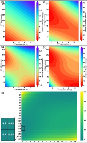
Table 2. The $R^2$ and MAE of a different order of polynomial regression model.

Number of Order	1st	2nd	3rd	4th	Alpha-4th
${\mathit{R}}^2$	0.2432	0.6348	0.7021	0.7159	0.6874
MAE	7.6481	5.6538	5.0238	4.8269	5.1363

Following optimisation of the 4^th-order polynomial model, an analysis was conducted on the printing error and its correlation with printing parameters. As shown in Figure 6(d), high print accuracy and minimal print errors are predominantly concentrated in regions with a UV light intensity of 20 and a UV exposure time of 10s or a UV light intensity of 100–150 and a UV exposure time of approximately 2s. Furthermore, Figure 6(e) illustrates the variation and distribution of printing errors with different printing parameters. Better printing errors can be obtained within the UV light intensity range of 15–20, UV exposure time between 10–15s, UV light intensity of 115–155, and UV exposure time of 1.5–3s. However, there are still a few negative predicted values, albeit not substantial. This indicates that the optimised model still suffers from overfitting, which may lead to generalisation. Given that the optimised 4^th-order polynomial model has $R^2$. and MAE of 0.6874 and 5.1363, respectively; this suggests that polynomial regression models are unsuitable for predicting high-precision printing accuracy in DLP. The model's performance may be restricted when the relationship between the input variables (i.e. printing parameters) and the output (i.e. predicted printing error) is non-linear. Moreover, the model's accuracy may be affected by missing values or outliers in the experimental data since polynomial regression models are sensitive to such issues. Lastly, if there are interaction effects between the training data's input variables, the polynomial model's final predictive performance may also be limited. Conversely, the ‘RF’ model can effectively handle non-linear relationships between inputs and outputs, missing values and outliers, and interaction effects. Furthermore, using RF models allows non-linear relationships between independent variables to be represented, enhancing their predictive capabilities compared to polynomial regression models.

After optimising the 4^th-order and getting the Alpha 4^th-order polynomial model, a comprehensive analysis was conducted to examine the relationship between printing errors and printing parameters. Figure 6(e) visually represents the variation and distribution of printing errors across different printing parameters. Superior printing errors can be achieved within the UV light intensity range of 15–20 and a UV exposure time of 10–15s, as well as a UV light intensity of 115–155 and a UV exposure time of 1.5–3s. However, it should be noted that a few negative predicted values are present, albeit not significant. This suggests that although the optimised model addresses overfitting, it may exhibit limited generalisation capabilities. The $R^2$ and MAE values of 0.6874 and 5.1363, respectively, for the Alpha 4^th-order polynomial model indicate that polynomial regression models are inadequate for accurately predicting high-precision printing accuracy in DLP. This limitation arises from the non-linear relationship between the input variables (i.e. printing parameters) and the output (i.e. predicted printing error). The performance of the model can also be compromised by missing values or outliers in the experimental data, as polynomial regression models are sensitive to such issues. Additionally, interaction effects between the input variables may further constrain the predictive power of the polynomial model.

3.1.2. Random forest model with fixed 50 µm layer thickness

The ‘RF’ model is employed in this study to predict the printing errors based on the input variables of UV light intensity and exposure time for various combinations. The model construction involves randomly selecting a subset of samples to create decision tree nodes, from which multiple decision trees are generated. These decision trees’ predictions are then averaged to yield the final RF prediction results. To further refine the data processing, two methods are employed for comparison. The first method utilises the raw data, while the second incorporates ‘Polynomial Features’ to capture interactions and non-linear relationships between the features, enhancing the model's performance and fit. The study analyses and compares the two data training models and their respective results to identify the most suitable prediction model. To ensure the construction of an accurate and reliable ‘RF’ model, it is essential to determine the optimal values for critical parameters such as n_estimators, max_depth, min_samples_split, and min_samples_leaf because these parameters significantly impact the performance and predictive capabilities of the model. Grid Search CV, a widely-used method for hyperparameter tuning, is employed to systematically explore different combinations of these parameters and identify the optimal combination that yields the best results [50, 51]. During the hyperparameter tuning process, Grid Search CV systematically explores various combinations of specified hyperparameter values and conducts cross-validation on each combination. By evaluating the performance of each combination, Grid Search CV identifies the model with the optimal performance and determines its corresponding best hyperparameters. Therefore, in this study, we employ the Grid Search CV method for hyperparameter tuning and employing cross-validation to divide the dataset into five folds, using one fold as the validation set and the remaining folds as the training set. This approach allows multiple evaluations of the model's performance, reducing reliance on a specific training set. By exhaustively searching through the parameter space, Grid Search CV assists in identifying the ideal set of parameters that maximises the model's accuracy and generalizability. This ensures that the model's performance is evaluated comprehensively across different data subsets, thus providing a more reliable measure of effectiveness. The results of the parameter optimisation process, including the chosen optimal values for n_estimators, max_depth, min_samples_split, and min_samples_leaf, are presented in Table 3. The average accuracy achieved through GridSearchCV is determined to be 0.8699, indicating that the model's average accuracy on the cross-validation data reaches 86.99%. This demonstrates the model's capability to perform well and generalise effectively across different data samples. By selecting the model with the best performance and its corresponding best hyperparameters, we can achieve optimal model performance and enhance the reliability and interpretability of our findings. This rigorous approach ensures that our conclusions are based on a well-optimised model that can effectively generalise to unseen data and provide robust insights into the studied phenomena.

Table 3. Optimal combination of parameters of the ‘Random Forest’ model.

Parameter	n_estimators	max_depth	min_samples_split	min_samples_leaf
Range	[100,200,500]	[None,5,10]	[2,5,10]	[1,2,4]
Result	200	10	5	2

The performance of the ‘RF’ models developed with and without the incorporation of ‘Polynomial Features’ was examined and compared, as shown in Figure 7(a,b). Both models exhibited similar prediction trends, with consistent error values and ranged across the predictions. However, distinct differences were observed in the prediction area between the two models. The ‘RF’ model constructed using the raw data showed clear boundary features in the prediction area, which deviated from the actual printing trend. This discrepancy suggests that the model's predictions may not accurately capture the non-linear relationship between the printing parameters and the desired outcomes. On the other hand, the ‘RF’ model that incorporated ‘Polynomial Features’ into the original data demonstrated a smoother prediction curve and a better fit with the actual prediction. This enhanced performance can be attributed to the ability of ‘Polynomial features’ to capture complex interactions and non-linear patterns within the data. On the analysis of curing theory, it is understood that an appropriate printing range should exhibit a gradual and continuous variation in curing energy as the light intensity or exposure time changes rather than abrupt jumps. Therefore, the ‘RF’ model incorporating ‘Polynomial Features’ aligned with this understanding and was selected as the final prediction model. The model chosen achieved a $R^2$ value of 0.8362, out-of-bag (OOB) is 0.8661, and there is an MAE value of 3.4786, as shown in Table 4. The high $R^2$ the value indicates a strong correlation between the predicted and actual printing outcomes, while the low MAE value suggests minimal average deviation between the predicted and actual printing errors. During the model training process, each decision tree within the ‘RF’ algorithm is trained using a bootstrap sample obtained from the original dataset. Notably, a subset of the data known as the out-of-bag (OOB) samples are excluded from the training of each decision tree. These OOB samples are then utilised to assess the model's performance by calculating their prediction accuracy. In our study, the OOB score of the model is determined to be 0.8661, indicating an average accuracy of 86.61% on the OOB samples. This high OOB score signifies the model's effectiveness in capturing underlying patterns and making accurate predictions. These metrics serve as indicators of the model's accuracy and performance. Similarly, the variation and distribution of printing errors under different printing parameters are visualised in Figure 7(c). Notably, the predictions indicate that lower light intensity and higher exposure time settings result in lower printing errors, aligning with the observed printing outcomes. This correspondence between the predicted and practical printing experience serves as further evidence supporting the scientific validity and practical utility of the Random Forest prediction model. Based on the robust performance of the selected ‘RF’ model, all subsequent experiments in this study were conducted using the best printing parameters obtained from this model. This approach ensures the experiments are carried out with optimised settings, maximising the chances of predicting print errors and achieving high-precision printing results.

Figure 7. Printing error and print parameter (a) Distribution relationship of ‘Polynomial Features’ data. (b) Distribution relationship of original data. (c) ‘RF’ model prediction error distribution (‘Polynomial Features’ data), unit: µm.

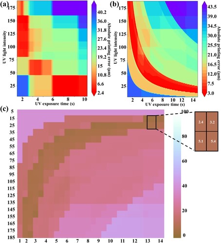
Table 4. Optimal printing parameters of ‘RF' Performance index parameters of ‘RF' based on part data (No layer thickness).

‘RF’	${\mathit{R}}^2$	MAE	OOB
Value	0.8362	3.4786	0.8661

3.1.3. Random forest model based on variety layer thickness

Having ensured the efficacy of the Random Forest model for 50 µm layer thicknesses, a comprehensive dataset with varying layer thicknesses was introduced to further refine the model's predictive capabilities under diverse printing conditions. Employing the grid search CV method facilitated the identification of optimal parameter combinations that yielded the best results, as depicted in Table 5. The average accuracy from GridSearchCV, recorded as 0.8708, attests to the model's robust performance and effective generalisation across diverse data samples. Additionally, Table 5 reveals the Random Forest prediction model's metrics, including an R^2 of 0.8500, an OOB of 0.8784, an MAE of 3.3029, and a confidence interval of 1.91 µm.

Table 5. Optimal printing parameters of ‘RF' Performance index parameters of ‘RF' based on part data (Including layer thickness).

‘RF’	${\mathit{R}}^2$	MAE	OOB
Value	0.8500	3.3029	0.8774

Figure 8(a) elucidates the nuanced distribution trends correlating different print layer thicknesses, UV light intensities, and exposure times with the resultant printing error. In conjunction with the printing error distribution pattern observed for a 50 µm layer thickness and the actual printing error variability, it becomes evident that the printing error prediction model manifests a non-linear, gradient-type variation under consistent exposure conditions and light intensities. The alterations in layer thickness induce a gradual and regular shift in the overall printing error distribution trend, emphasising the practicality and authenticity of the prediction model. Of significance is the observation that the overall printing error escalates when the layer thickness descends below 20 µm, attributable to the inherent limitations of the resin utilised. This decrease in printing accuracy underscores the need for high-precision resins. To substantiate the indispensability of the printing process optimisation utilising the prediction model, a comparative analysis was conducted using both resin-recommended and model-optimised printing parameters on a bespoke high-precision DLP printer. Notably, over-curing, as illustrated in Figure 8(b), results in an expanded width of the designed structure, an augmented printing error, and unintended curing of surrounding resin due to excessive energy. Conversely, employing optimised parameters, as demonstrated in Figure 8(c), ensures heightened structural accuracy, minimised printing errors, and clear structural edges, unequivocally affirming the necessity of parameter optimisation. To rigorously validate the accuracy of the prediction model, a search algorithm randomly selected two printing parameters with a 30 µm layer thickness and a prediction error within 10 µm from 10,360,000 data. The parameters derived from this process, detailed in Table 6, exhibited prediction errors of 7.72 and 7.77 µm, closely aligning with the actual printing errors of 6.23 and 6.34 µm. Figure 8(d) illustrates that these parameters harmonise with the overall trend of change, with the deviation of the actual printing value from the predicted printing error falling within the ‘confidence interval’ of 1.46 µm. This alignment within the confidence interval substantiates the validity and generalizability of the prediction model. These findings highlight the utility of the model and its critical role in guiding effective parameter optimisation, leading to improved printing accuracy.

Figure 8. (a) The distribution relationship between print parameters and printing error. (b) Print structure with normal print parameters. (c) Print structure with optimized print parameters based ‘RF’ model. (d) Actual printed widths after optimisation based on the ‘RF’ model (layer thickness 30 µm).

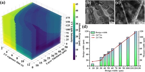
Table 6. Optimal printing parameters of ‘RF' model with 30 µm layer thickness.

Layer Thickness	Light Intensity	Exposure Time	Predict Error	Print Error
30µm	24	7.1s	7.72µm	6.23µm
30µm	21	7.0s	7.77µm	6.34µm

3.2 Printing high-precision microfluidic mold A rigorous exploration into the enduring validity and adaptability of the RF-based model in real-world contexts was meticulously undertaken to ensure its versatility across diverse printing scenarios. The initial phase involved the precise determination of the printing layer thickness in strict adherence to the design specifications of the microfluidic master molds with 2.5D cross sections (a Y-type mixer) and multi-level heights (a Herringbone mixer). Subsequently, the meticulously optimised RF model-predicted printing parameters were implemented for high-precision printing and carried out a thorough assessment of the accuracy and validity of the model's predictions. This comprehensive analysis attests to the resilience and pragmatic applicability of the RF-based model across a spectrum of microfluidic printing scenarios.

As shown in Table 6, the height of the Y-shaped is 100 µm, and herringbone structures embody a double-layer configuration, featuring a first layer height of 100 µm and a second layer height of 50 µm, with a minimum feature size of 20 µm for the Y-shaped structure and 21 µm for the herringbone structure. As a result, as the most commonly used print layer thickness in DLP printing 50 µm was selected as the final print layer thickness, and the corresponding predicted printing parameters are shown in Table 7.

Table 7. Predict parameters of the printing structure.

Structure	Layer thickness (µm)	Light intensity	Exposure time (s)	Predict error (µm)
Y-type	50	18	10.7	1.95
Herringbone	50	18	10.7	1.95

3.2. Printing Y-type and herringbone structure mold

Using the printing parameters predicted by the optimised ‘RF’ model, high-precision printing was conducted to validate the accuracy and efficacy of the model's predictions, and the Y-type and Herringbone structures were used to evaluate the performance of the ‘RF’ model.

3.2.1. Y-type structure

The Y-type structure is widely used in microfluidics and consists of a main channel and two side channels that meet at a Y-shaped junction. When fluids with different flow rates are introduced into the main and two side channels, the fluids will merge at the intersection and mix efficiently due to the formation of vortices and eddies. Figure 9(a) depicts the Y-type structure with design dimensions provided in Table 6. The structure is 10 mm in length with a fixed height of 100 µm and a varying width of 20, 25, and 30 µm, resulting in a depth-to-width ratio that ranges from 3.3:1 to 5:1. Using the optimal printing parameters for UV light intensity and exposure time from the ‘RF’ model (c.f. Table 4: 18, 10.7s), the Y-type structure is successfully fabricated via our customised DLP printing system. A 5-minute sonication in Isopropyl alcohol (IPA) solution at 25°C removes residual resin from the surface of the structure and improves its transparency and surface quality. The post-processing of the Y-type structure involves UV curing using a UV lamp (Phrozen, Taiwan) to enhance its mechanical properties, followed by immersion in distilled water for 10 min. After completion of the post-processing procedure, the print structure is promptly characterised.

Figure 9. Y-type structure (a) Schematic diagram of the Y-shaped structure. (b) Printing error of different Y-type structures. (c) The surface roughness of different Y-type structures. (d) The height and 2D profile of Y-type 20 µm structure. (e) The SEM image of Y-type 20 µm structure. (f) The height and 2D profile of Y-type 25 µm structure. (g) The SEM image of Y-type 25 µm structure. (h) The height and 2D profile of Y-type 30 µm structure. (i) The SEM image of Y-type 30 µm structure.

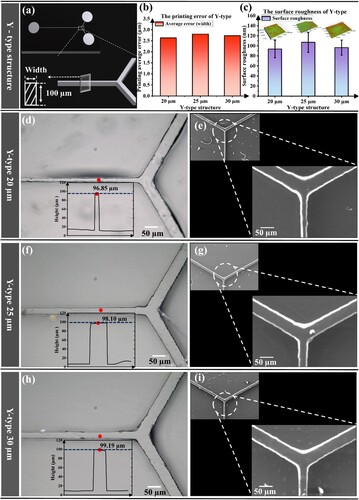
The present study employed an optical microscope with 500× magnification to measure the width of various Y-type structures and obtain the average printing error. As shown in Figure 9(b), all the printed structures displayed less than 3 µm errors, indicating that the optimal printing parameters derived from the ‘RF’ model achieved satisfactory printing accuracy. To assess the print result quantitatively, surface roughness was measured using a Bruker NPFLEX white light interferometer equipped with a 0.025 mm short-wavelength Gaussian cut-off filter. The ‘Arithmetic Average Roughness’ (Ra) was determined to be approximately 100 nm (Figure 9(c)) using the ‘Stylus analysis’ module. The 3D profile of Y-type structures with widths of 20 µm (Figure 9(d, e)), 25 µm (Figure 9(f, g)), and 30 µm (Figure 9(h, i)) were examined using SEM. The SEM photographs confirmed that the optimal printing parameters enabled the successful printing of Y-type structures with various widths and distinct 3D features. To measure the height of the Y-type structure, the 3D scanning function of the optical microscope was employed, with Y-type structures of 20, 25, and 30 µm having heights of 96.85, 98.10, and 99.19 µm, respectively. The average height of these printed structures was 98.04 µm, demonstrating high accuracy in printing height. The red dots in Figure 9(d,f,h) depict the height scanning points, and the contour maps and contour data were acquired from the ‘3D display’ module of the optical microscope. Overall, the optimised parameters allowed for the high-precision printing of Y-type structures with a minimum feature size of 20 µm.

3.2.2. Herringbone structure

HBS are ubiquitous in microfluidic devices and have diverse applications in biomedicine, such as drug delivery[52] and nanoparticle synthesis[53, 53]. The inherent vortices and secondary flows generated by the herringbone pattern substantially augment mixing efficiency and decrease the diffusion length between fluids. Moreover, HBS can be incorporated into microfluidic devices aimed at cell sorting and separation, as the intricate fluid flow patterns engendered by this structure can bolster the precision and efficacy of these procedures.

HBS is found in microfluidic devices comprising two layers, with the fishbone structure forming the second layer. As shown in Figure 10(a), the HBS is an array structure with each bevelled edge inclined at 45 degrees to the edge and a top height of 50 µm. The HBS interval distance is fixed at 150 µm, while the widths of 30, 40, 50, and 150 µm intervals correspond to the true design width of 21.1, 28, 35.4, and 106.1 µm, respectively, due to their 45 degrees angle. These dimensions are reported in Table 8. The study employed our DLP printing system to print the HBS structures and measured the average printing error with an optical microscope under optimal printing parameters. The results showed a printing error of approximately 3 µm for width and 1 µm for interval, as depicted in Figure 10(b). The surface roughness of HBS was also measured using a Bruker NPFLEX white light interferometer, which revealed a Ra of approximately 100 nm (Figure 10(c)). The 2D diagrams of the 30, 40, and 50 µm/150 µm structures in Figure 10(d,f,h), respectively, were characterised using the optical microscope ‘3D display’ module, with the red dots representing the height scanning points. The design height was 50 µm, with an average measured height of 49.94 µm and an average printing error below 0.5 µm. Additionally, SEM was employed to characterise the different HBS structures in the 3D diagram, revealing that the line width of the structure increased from Figure 10(e,g,i). The study confirmed the feasibility of optimising print parameters and achieving high-precision printing through machine learning. HBS structures with a minimum feature size of 21 µm can be successfully printed using the optimised print parameters with a customised DLP printing system. This study provides valuable insights to researchers on how to efficiently print with a novel printing system and resins and promptly identify optimal printing parameters to meet various printing requirements and applications.

Figure 10. HBS (a) Schematic diagram of the HBS. (b) Printing error of different HBS. (c) The surface roughness of different HBS. (d) The height and 2D profile of HBS 30/150 µm structure. (e) The SEM image of HBS 30/150 µm structure. (f) The height and 2D profile of HBS 40/150 µm structure. (g) The SEM image of HBS 40/150 µm structure. (h) The height and 2D profile of HBS 50/150 µm structure. (i) The SEM image of HBS 50/150 µm structure.

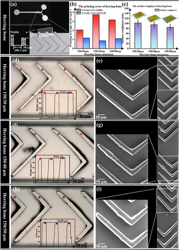
Table 8. Design parameters of the printing structure.

Structure	Height	Structure-1	Structure-2	Structure-3
Y-type	100µm	20µm	25µm	30µm
Herring bone	Bottom layer: 100µm Top layer: 50 µm	30/150µm (21.1/106.1 µm)	40/150µm (28/106.1 µm)	50/150µm (35.4/106.1 µm)

3.2.3. Printing mold and manufacturing PDMS chips

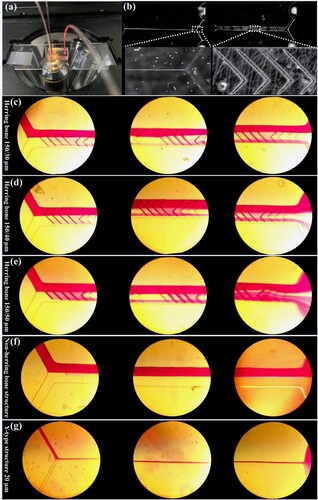
To fabricate the PDMS microfluidic chip, a mixture of Sylgard 184 and RTV 615 was prepared and treated under a vacuum for 40 min to remove any trapped air bubbles. Subsequently, the DLP printed molds were placed in glass Petri dishes, coated with a release agent, and baked on a heated table at 60°C for 4 h to ensure complete demolding of the mold surface. To create the microfluidic channels, PDMS was poured over the molds and cured at 45°C for 8 h. The cured PDMS replica was separated carefully from the molds, underwent Plasma surface treatment, and finally bonded to a glass sheet, producing the final microfluidic chip. To demonstrate the efficacy of machine learning-based parameter optimisation to achieve precise printing, a set of PDMS microfluidic chips were fabricated through our custom-made DLP printing system combined with optimised printing parameters to print Y-shaped and HBS as molds. This approach validates the feasibility of printing molds with optimal parameters obtained through machine learning and provides a practical method for fabricating microfluidic devices with complex structures at high resolution.

In this study, microfluidic chips were fabricated using various molds, such as HBS with widths of 30/150 µm, 40/150 µm, and 50/150 µm, as well as non-herringbone pattern structures and a Y-type structure with a width of 20 µm. As shown in Figure 11(a), the mixing effects of different solutions within the microfluidic chips were observed subsequently. This proof-of-concept approach demonstrates the applicability and universality of the optimised parameters derived from the ‘RF’ model for fabricating different microfluidic devices with complex structures at high resolution. The PDMS chip ware synthesised and immersed in the demolded HBS-Y-type structure, followed by evacuation for 40 min and heating at 60 degrees on a hot table for 12 h. The PDMS chip was then plasma-treated, bonded, and characterised using microscopy. The microstructure of the PDMS chip (Y-type 20 µm with 30/150 µm HBS) was found to be intact (Figure 11(b)), indicating successful fabrication and usability for subsequent experiments. To assess the effect of the printed molds, rhodamine B was mixed with ethanol and used as a solution in the fabricated PDMS microfluidic chips that were placed under a microscope for real-time synthesis observation. The results showed that the 50/150 HBS structure provided the best mixing efficiency, with the solution being almost completely mixed by the time it reached the end of the chip (Figure 11(e)). As the feature size decreased, the mixing became less effective, and the 40/150 structure (Figure 11(d)) mixed significantly better than the 30/150 (Figure 11(c)). This observation indicates that different sizes of the same structure have different mixing efficiencies. Additionally, the non-HBS structure had no characteristic size, and no mixing occurred throughout the solution, demonstrating that the printing results effectively promote solution mixing (Figure 11(f)). Moreover, the Y-type structure showed the worst and negligible mixing efficiency compared to the HBS structure, indicating that different structures have different mixing efficiencies (Figure 11(g)). This experiment validates the accuracy of the printed molds after parameter optimisation. The practicality of printing molds is demonstrated by fabricating PDMS chips and observing the solution mixing efficiency with different structures while further validating the scientific and general nature of the optimisation parameters derived from the machine learning model. This provides a novel way of thinking and achieving fast and precise DLP printing.

Figure 11. (a) PDMS microfluidic chip solution mixing experiments. (b) Y-type 20 µm and HBS 30/150 µm. (c-g) Solution Mixing of different structures: from the beginning, middle, and end of the chip; (c) HBS 30/150 µm structure, (d) HBS 40/150 µm structure, (e) HBS 50/150 µm structure, (f) Non-HBS structure, (g) Y-type 20 µm structure.

3.3. Printing TPMS structure-based ‘RF’model

Microfluidic molds, despite necessitating high precision printing for the smallest feature size, inherently represent 2.5D structures within the strict confines of their definition. They do not exhibit the intricate characteristics of complex spatial 3D structures. Triple-periodic minimal surfaces (TPMS) structures, inspired by lattice materials, have emerged as a dynamic and promising avenue of exploration in the additive manufacturing domain. Their unique attributes, guided by stringent requirements in terms of porosity, volume ratio, and surface area ratio, propel them into a distinctive realm of research within the additive manufacturing landscape. Unlike conventional structures, TPMS structures demand meticulous attention to overall fabrication accuracy. The intricate nature of high-precision TPMS structures presents a formidable challenge in the realm of 3D printing. The quest for optimal printing extends beyond the faithful reproduction of TPMS void structures; it necessitates the steadfast preservation of consistent printing accuracy across the diverse scales inherent to the dynamic changes within TPMS structures. Therefore, TPMS structures were chosen to print as an experiment to validate the model.

Firstly, ‘RF’ predict model guide, which pinpointed optimal printing parameters: UV intensity of 20, an exposure time of 9.38 s, and a layer thickness of 48 microns as parameters that theoretically result in the smallest predicted print error, theoretically reaching as low as 0 µm. Then, as detailed in Table 9, the Gyroid and Diamond structures were set to a height of 480 µm, with the Gyroid's line width linearly increasing from 20 µm to 190 µm and the Diamond structure varying linearly from 20 µm to 150 µm. Upon obtaining the optimal printing parameters, the printing process was initiated. As depicted in Figure 12(a), the Gyroid and Diamond structures were successfully printed using the model-predicted parameters. Figure 12(b,c) showcase the intricate Diamond and Gyroid 3D structures, both presenting complex hollow features that place significant demands on the printing process. Figures 12(d-f) specifically illustrate the TPMS-Diamond structure. These figures highlight the continuous linear thickening of the Diamond structure while maintaining an excellent structural void ratio. Figure 9(f) emphasises the smallest structure of the Diamond, measuring 20 µm. Following parameter optimisation, the Diamond structure achieved remarkable accuracy, with a final overall printing error of only 1.35 µm. Similarly, Figure 12(g–i) illustrates the Gyroid structure, showcasing its complex features in both vertical and horizontal directions. Figure 12(i) specifically illustrates the minimum feature size of the Gyroid structure at 20 µm. Despite the Gyroid's varying feature size from 20 to 180 µm, the printing error remained consistently low at 1.42 µm after printing with the optimised parameters, truly attaining high-precision printing of these intricate and complex structures. Employing the prognostications print parameters of the ‘RF’ model, the successful realisation of precise printing for multi-layered TPMS-Gyroid and TPMS-Diamond structures, inclusive of intricate cavity formations, has been attained. Notably, the management of the overall printing error within a stable threshold of 1.5 µm throughout the progression from larger to smaller structures underscores the robustness and practicality of the printing parameters derived from the ‘RF’ prediction model. This substantiates the viability of the model-derived parameters as a tangible and effective solution for the intricate realm of high-precision microstructure printing.

Figure 12. (a) Printed ‘Diamond’ (Left) and ‘Gyroid’ (Right) 3D structures. (b) Diamond 3D model. (c) Gyroid 3D model. (d-f) The SEM images of ‘Diamond’ 3D structures; (d) Vertical characteristics of the ‘Diamond’ structure, (e): Horizontal characteristics of the ‘Diamond’ structure. (f) Minimum characteristic structure of the ‘Diamond’ structure. (g-i) The SEM images of ‘Gyroid’ 3D structures. (g) Vertical characteristics of the ‘Gyroid’ structure (h) Horizontal characteristics of the ‘Gyroid’ structure. (i) Minimum characteristic structure of the ‘Gyroid’ structure.4 Conclusions

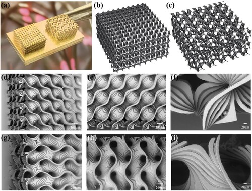
Table 9. Design parameters of TPMS structures.

TPMS Structure	Layer thickness (µm)	Light intensity	Exposure time	Height (µm)	Minimum Feature Size(µm)	Maximum Feature Size(µm)	Print Error(µm)
Gyroid	48	20	9.38s	480	20	190	1.35
Diamond	48	20	9.38s	48	20	15	1.42

Conclusion

This study developed a machine learning approach to resolve the challenge of high-precision microstructure printing using DLP with the typical application in the microfluidic area and expanded applications in complex TPMS structure fabrication. The major achievements of this study are high-precision printing with a minimum feature size of 20 µm and controlled printing error using a customised DLP printing system combined with a machine learning model:

• Firstly, we have developed a high-precision DLP printing system with a theoretical projection resolution of 5.4 µm. This customised DLP system allows for adjustable UV light intensity, exposure time and layer thickness as key control parameters.

• Secondly, we designed a star pattern micro structure covering most microfluidic feature dimensions and conducted a comprehensive set of experiments to establish machine-learning prediction models, Polynomial regression and ‘RF’, under varying UV light intensities, and exposure times and layer thickness. The ‘RF’ model demonstrated significantly more robust predictive capability (: 0.8362, OOB:0.8661, MAE: 3.4786). Based on the ‘RF’ prediction model, we determined the optimal printing parameter that minimises prediction errors by searching within the model;

• Thirdly, we designed and fabricated Y-type and HBS microfluidic mixers to validate the printing accuracy based on machine learning prediction. The results revealed that our customised printing system successfully achieved the printing of microstructures with a minimum feature size of 20 µm. Furthermore, the printing error of these structures was effectively controlled below 2.3 µm, while the surface roughness approached 100 nm. These results confirm the scientific and practical validity of the optimal printing parameters obtained from the random forest prediction model, addressing the challenges associated with high-precision DLP printing. Remarkably, distinct mixing behaviours were observed in microfluidic chips of different sizes for both the Y-type and HBS designs, highlighting the influence of microstructure size on fluid dynamics. This further validate the approach that high precision 3D printing can be used for microfluidic device prototyping.

• Lastly, the derivation of optimal printing parameters was accomplished by inputting the ‘full dataset’ into the ‘RF’ prediction model, facilitating the successful fabrication of intricate TPMS structures. This pivotal step signifies an expansion of the prediction model's applicability from 2.5D to intricate 3D structures, particularly TPMS-Gyroid and TPMS-Diamond, featuring a minimum feature size of 20 µm.

Acknowledgement

This study employed machine learning models to establish the relationship between print input parameters and errors, representing an initial exploration. Besides printing parameters, the material significantly influences DLP printing accuracy. A more comprehensive investigation is warranted to fully comprehend the intricate interplay between print materials, material composition, material ratios, print parameters, and the resulting print errors, this is also an important direction for our next research. Such endeavours hold promise for revolutionising the field of high-precision manufacturing by providing precise error prediction and facilitating the advancement of rapid and high-precision manufacturing processes. I would like to extend our heartfelt appreciation to Dr. Nan Zhang and Dr. Jinghang Liu for their exceptional guidance and unwavering support throughout the entirety of this process. Additionally, we are deeply grateful to Prof. Michael Gilchrist, Dr. Ruihai Dong for their meticulous review and insightful feedback on this manuscript prior to its submission to the journal. Furthermore, we would like to acknowledge the generous financial support provided by the European Union's Horizon 2020 Research and Innovation Programme under the Marie Skłodowska-Curie, Science Foundation Ireland (SFI) and Enterprise Ireland.

Disclosure statement

No potential conflict of interest was reported by the author(s).

Data availability statement

There is no data set associated with this paper.

Additional information

Funding

Funding that has been provided by the European Union’s Horizon 2020 Research and Innovation Programme under the Marie Skłodowska-Curie (Grant Agreement No. 956097); the Science Foundation Ireland (SFI) (No. 22/NCF/FD/10914 and 20/FIP/PL/8741); and Enterprise Ireland (CF-2021-1635-P).

References

- Scott SM, Ali Z. Fabrication methods for microfluidic devices: an overview. Micromachines. 2021;12(3). doi: 10.3390/mi12030319
- Hansen CL, Skordalakes E, Berger JM, et al. A robust and scalable microfluidic metering method that allows protein crystal growth by free interface diffusion. Proc Natl Acad Sci U S A. 2002;99(26):16531–16536. doi: 10.1073/pnas.262485199
- Takayama S, Ostuni E, LeDuc P, et al. Subcellular positioning of small molecules. Nature. 2001;411(6841):1016–1016. doi: 10.1038/35082637
- Guo MT, Rotem A, Heyman JA, et al. Droplet microfluidics for high-throughput biological assays. Lab Chip. 2012;12(12):2146–2155. doi: 10.1039/c2lc21147e
- Xinhui Wang JL, Zhang Y, Kristiansen PM, et al. Advances in precision microfabrication through digital light processing: system development, material and applications. Virtual Phys Prototyp. 2023;18(1). doi: 10.1080/17452759.2023.2248101
- Whitesides GM. The origins and the future of microfluidics. Nature. 2006;442(7101):368–373. doi: 10.1038/nature05058
- Wei CW, Cheng JY, Huang CT, et al. Using a microfluidic device for 1 microl DNA microarray hybridization in 500 s. Nucleic Acids Res. 2005;33(8):e78. doi: 10.1093/nar/gni078
- Zhang P, He M, Zeng Y. Ultrasensitive microfluidic analysis of circulating exosomes using a nanostructured graphene oxide/polydopamine coating. Lab Chip. 2016;16(16):3033–3042. doi: 10.1039/c6lc00279j
- Reyes DR, Iossifidis D, Auroux P-A, et al. Micro total analysis systems. 1. Introduction, theory, and technology. Anal Chem. 2002;74(12):2623–2636. doi: 10.1021/ac0202435
- Duffy DC, McDonald JC, Schueller OJA, et al. Rapid prototyping of microfluidic systems in poly (dimethylsiloxane). Anal Chem. 1998;70(23):4974–4984. doi: 10.1021/ac980656z
- Amini A, Guijt RM, Themelis T, et al. Recent developments in digital light processing 3D-printing techniques for microfluidic analytical devices. J Chromatogr A. 2023;1692:463842. doi: 10.1016/j.chroma.2023.463842
- Gonzalez G, Roppolo I, Pirri CF, et al. Current and emerging trends in polymeric 3D printed microfluidic devices. Add Manuf. 2022;55. doi: 10.1016/j.addma.2022.102867
- Yazdi AA, Popma A, Wong W, et al. 3D printing: an emerging tool for novel microfluidics and lab-on-a-chip applications. Microfluid Nanofluid. 2016;20:3. doi: 10.1007/s10404-016-1715-4
- Kim P, Lee SE, Jung HS, et al. Soft lithographic patterning of supported lipid bilayers onto a surface and inside microfluidic channels. Lab Chip. 2006;6(1):54–59. doi: 10.1039/b512593f
- Zheng X, Lee H, Weisgraber TH, et al. Ultralight, ultrastiff mechanical metamaterials. Science. 2014;(6190):1373–1377. doi: 10.1126/science.1252291
- Au AK, Huynh W, Horowitz LF, et al. 3D-Printed Microfluidics. Angew Chem Int Ed Engl. 2016;55(12):3862–3881. doi: 10.1002/anie.201504382
- Shallan AI, Smejkal P, Corban M., et al. 2014. Cost-effective three-dimensional printing of visibly transparent microchips within minutes. Anal Chem. (6):3124–3130. doi: 10.1021/ac4041857
- Macdonald NP, Cabot JM, Smejkal P, et al. Comparing microfluidic performance of three-dimensional (3D) printing platforms. Anal Chem. 2017;(7):3858-3866. doi: 10.1021/acs.analchem.7b00136
- Razavi Bazaz S, Rouhi O, Raoufi MA, et al. 3D Printing of inertial microfluidic devices. Sci Rep. 2020;(1):5929. doi: 10.1038/s41598-020-62569-9
- Razavi Bazaz S, Kashaninejad N, Azadi S, et al. Rapid softlithography using 3D-printed molds. Adv Mat Technol. 2019;4(10). doi: 10.1002/admt.201900425
- Gong H, Bickham BP, Woolley AT, et al. Custom 3D printer and resin for 18 mu m x 20 mu m microfluidic flow channels. Lab Chip. 2017;17:2899–2909. doi: 10.1039/c7lc00644f
- Bucciarelli A, Paolelli X, De Vitis E, et al. VAT photopolymerization 3D printing optimization of high aspect ratio structures for additive manufacturing of chips towards biomedical applications. Add Manufact. 2022;60. doi: 10.1016/j.addma.2022.103200
- Cheng L, De Vos J, Zhao P, et al. Examining non-linear built environment effects on elderly’s walking: a random forest approach. Transp Res D Transp Environ. 2020;88. doi: 10.1016/j.trd.2020.102552
- Caraviello DZ, Weigel KA, Craven M, et al. Analysis of reproductive performance of lactating cows on large dairy farms using machine learning algorithms. J Dairy Sci. 2006;89(12):4703–4722. doi: 10.3168/jds.S0022-0302(06)72521-8
- Vinay A, Shekhar VS, Rituparna J, et al. Cloud based big data analytics framework for face recognition in social networks using machine learning. Procedia Comput Sci. 2015;50:623–630. doi: 10.1016/j.procs.2015.04.095
- He H, Yang Y, Pan Y. Machine learning for modeling of printing speed in continuous projection stereolithography. Paper presented at the 2018 International Solid Freeform Fabrication Symposium. 2018.
- You S, Guan J, Alido J, et al. Mitigating scattering effects in light-based three-dimensional printing using machine learning. J Manuf Sci Eng. 2020;142(8). doi: 10.1115/1.4046986
- Sun X, Yue L, Yu L, et al. Machine learning-evolutionary algorithm enabled design for 4D-printed active composite structures. Adv Funct Mater. 2021;32:10. doi: 10.1002/adfm.202109805
- Zhao B, Zhang M, Dong L, et al. Design of grayscale digital light processing 3D printing block by machine learning and evolutionary algorithm. Compos Commun. 2022;36. doi: 10.1016/j.coco.2022.101395
- Kiratitanaporn W, Guan J., Berry DB, et al. Multimodal three-dimensional printing for micro-modulation of scaffold stiffness through machine learning. Tissue Eng Part A. 2023. doi: 10.1089/ten.TEA.2023.0193
- Montgomery SM, Demoly F, Zhou, K, et al. Pixel-level grayscale manipulation to improve accuracy in digital light processing 3D printing. Adv Funct Mater. 2023;33(17). doi: 10.1002/adfm.202213252
- Jacobs PF. Rapid Prototyping Manufacturing Fundamentals of StereoLithography by Jacobs P.F. (z-lib.org).pdf (Vol. “Working cure model” Most classical). 1992.
- Gong H, Beauchamp M, Perry S, et al. Optical approach to resin formulation for 3D printed microfluidics. RSC Adv. 2015;5:106621–106632. doi: 10.1039/C5RA23855B
- Li Y, Mao Q, Li X, et al. High-fidelity and high-efficiency additive manufacturing using tunable pre-curing digital light processing. Add Manufact. 2019. doi: 10.1016/j.addma.2019.100889
- Benjamin AD, Abbasi R, Owens M, et al. Light-based 3D printing of hydrogels with high-resolution channels. Biomed Phys Eng Express. 2019;5(2). doi: 10.1088/2057-1976/aad667
- Swineharf DF. Beer-lambert law.pdf. J Chem Educ. 1962. doi: 10.1021/ed039p333
- Smith PF, Ganesh S, Liu P. A comparison of random forest regression and multiple linear regression for prediction in neuroscience. J Neurosci Methods. 2013;220(1):85–91. doi: 10.1016/j.jneumeth.2013.08.024
- Ostertagová E. Modelling using polynomial regression. Procedia Eng. 2012;48:500–506. doi: 10.1016/j.proeng.2012.09.545
- Aczel AD. Complete Business Statistics (Vol. p. 1056). ISBN 0-256-05710-8. 1989.
- Ostertagová E. Applied Statistic (in Slovak) (Vol. p. 161,). Elfa Košice, Slovakia: SBN 978-80-8086-171-1. 2011.
- Breiman L. Random forests. Mach Learn. 2001;45:5–32. doi: 10.1023/A:1010933404324
- Guo L, Chehata N, Mallet C, et al. Relevance of airborne lidar and multispectral image data for urban scene classification using Random Forests. ISPRS J Photogramm Remote Sens. 2011;66(1):56–66. doi: 10.1016/j.isprsjprs.2010.08.007
- Rodriguez-Galiano VF, Chica-Rivas M. Evaluation of different machine learning methods for land cover mapping of a Mediterranean area using multi-seasonal Landsat images and Digital Terrain Models. Int J Digital Earth. 2014;7(6):492–509. doi: 10.1080/17538947.2012.748848
- Rodriguez-Galiano V, Sanchez-Castillo M, Chica-Olmo M, et al. Machine learning predictive models for mineral prospectivity: An evaluation of neural networks, random forest, regression trees and support vector machines. Ore Geol Rev. 2015;71:804–818. doi: 10.1016/j.oregeorev.2015.01.001
- Breiman L. Bagging predictors. Mach Learn. 1996;24:123–140.
- Ahangar-Asr A, Faramarzi A, Mottaghifard N, et al. Modeling of permeability and compaction characteristics of soils using evolutionary polynomial regression. Comput Geosci. 2011;37(11):1860–1869. doi: 10.1016/j.cageo.2011.04.015
- Hu J, Szymczak S. A review on longitudinal data analysis with random forest. Brief Bioinform. 2023;24(2). doi: 10.1093/bib/bbad002
- Sun Y, Cheng H, Zhang S, et al. Prediction & optimization of alkali-activated concrete based on the random forest machine learning algorithm. Constr Build Mater. 2023;385. doi: 10.1016/j.conbuildmat.2023.131519
- Ahmad GN, Fatima H, Ullah S, et al. Efficient medical diagnosis of human heart diseases using machine learning techniques with and without GridSearchCV. IEEE Access 2022;10:80151–80173. doi: 10.1109/ACCESS.2022.3165792
- Ranjan GSK, Verma AK, Radhika S. K-nearest neighbors and grid search cv based real time fault monitoring system for industries. 2019 IEEE 5th international conference for convergence in technology (I2CT), IEEE, 2019.
- Shin H, Lee HJ, Chae U, et al. Neural probes with multi-drug delivery capability. Lab Chip. 2015;15(18):3730–3737. doi: 10.1039/C5LC00582E
- Maeki M, Saito T, Sato Y, et al. A strategy for synthesis of lipid nanoparticles using microfluidic devices with a mixer structure. RSC Adv. 2015;5(57):46181–46185. doi: 10.1039/C5RA04690D
- Zhigaltsev IV, Belliveau N, Hafez I, et al. Bottom-up design and synthesis of limit size lipid nanoparticle systems with aqueous and triglyceride cores using millisecond microfluidic mixing. Langmuir. 2012;28(7):3633–3640. doi: 10.1021/la204833h