Revealing formation mechanism of end of process depression in laser powder bed fusion by multi-physics meso-scale simulation

ABSTRACT

Unintended end-of-process depression (EOPD) commonly occurs in laser powder bed fusion (LPBF), leading to poor surface quality and lower fatigue strength, especially for many implants. In this study, a high-fidelity multi-physics meso-scale simulation model is developed to uncover the forming mechanism of this defect. A defect-process map of the EOPD phenomenon is obtained using this simulation model. It is found that the EOPD formation mechanisms are different under distinct regions of process parameters. At low scanning speeds in keyhole mode, the long-lasting recoil pressure and the large temperature gradient easily induce EOPD. While at high scanning speeds in keyhole mode, the shallow molten pool morphology and the large solidification rate allow the keyhole to evolve into an EOPD quickly. Nevertheless, in the conduction mode, the Marangoni effects along with a faster solidification rate induce EOPD. Finally, a ‘step’ variable power strategy is proposed to optimise the EOPD defects for the case with high volumetric energy density at low scanning speeds. This work provides a profound understanding and valuable insights into the quality control of LPBF fabrication.

KEYWORDS:

• Additive manufacturing
• laser powder bed fusion
• meso-scale simulation
• end-of-process depression
• multi-physics simulation

1. Introduction

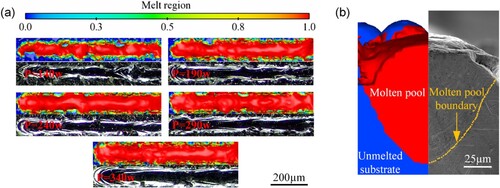
Laser powder bed fusion (LPBF) is an important branch of metal additive manufacturing (AM) technology, where a laser beam is used as a heat source to selectively melt pre-paved metal powders to form the designed geometry of a 3D model. Because of the fast-scanning speed and small laser beam diameter, the LPBF formed track is slender and usually with good quality, showing the potential of manufacturing complex metallic structures. This capability undoubtedly expands the prospects of LPBF technology, but also puts forward higher requirements for its moulding quality [1,2]. Therefore, the defect optimisation of LPBF technology has always been a hot topic [3,4]. However, inappropriate process parameters or poor powder bed quality inevitably lead to undesirable surface issues during LPBF [5], which is one of the current challenges of this technology. These defects induce lower fatigue strengths of AMed parts than traditionally manufactured parts with smoother surface finishes [6,7]. In many practical applications, especially biomedicine, high surface roughness is very detrimental to the implant, e.g. damage to host bone through stress shielding [8], against cell migration speed on surfaces [9] and decreasing the in vivo reactions between the surfaces and cells or proteins [10]. Concave surface or surface depression on the melt track is a kind of severe surface defect. It is harmful to the fusion between layers and can trap powder particles after the subsequent powder-spreading process. These trapped particles cannot be melted because of the fact that part of laser rays is reflected back to the gas when irradiating on the slope surface of depression [11]. For biomedical applications, depressions can easily form agglomeration of unmelt powders in the edges of the pores of porous structures such as alternative bone scaffolds (see Figure 1(a)). Regarding the clinical concerns of bioinert nature, this defect limits the interaction with bone to establish fixation.

Figure 1. (a) As-printed graded triply periodic minimal surface (TPMS) scaffolds by selective laser melting (SLM) [10]. (b) The EOPD phenomenon was observed in the experiment (P = 340 W, V = 1.06 m/s).

To reduce the negative effect of the drawback, many researchers have investigated the formation mechanisms of the concave surface. Li et al. [12,13] found that wetting behaviour of the molten pool driven by Marangoni force and recoil pressure induced the cavity further penetration and caused the concave surface. Guo et al. [14,15] claimed that the combination effect of Marangoni force, gravity and recoil pressure resulted in severe spattering and formed a concave surface. Li et al. [16] focused on the Marangoni effect on the depression formation. They found that negative and small temperature coefficient of surface tension was the main reason causing the depression after solidification. A typical concave surface defect which always occurs at the end of a track is called end-of-process depression (EOPD). As shown in Figure 1(b), after grinding off the end of the melt track by 0.05 mm to expose the cross-section, it is found that an approximate ‘W’ shaped concave region is formed on the upper surface of the melt track here. In terms of size, EOPD is larger than pores, which is observed in the study of Aboulkhair et al. [17]. Thijs et al. [18] formed a massive AlSi10Mg sample using LPBF technology and characterised it accordingly. The results showed that at the top of the sample, there was often a depression at the end of the track similar with EOPD, which they called ‘open pores’. They found that the open porosity or EOPD could still exist when multi-layer and multi-track scanning was performed. Qiu et al. [19] observed spherical pore defects and believed that their cause was incomplete remelting of the previous layer. That means EOPDs are not only limited to the surface quality mentioned in the previous paragraph, but also likely to evolve into real pores that are difficult to be removed internally during the subsequent printing process, thereby affecting the density of the component. In this regard, the EOPD defect becomes a critical issue which negatively influences the forming quality of LPBF components. In general, although some studies have found or involved EOPD defects, there is no systematic description of its formation mechanism and optimisation methods.

High-fidelity multi-physics simulation is an effective way to study the LPBF process and defect formation. Many powerful simulation models have been developed by the researchers all around world. The mainstream models can be categorised into three types, which are model without considering powder bed morphology and fluid flow, model considering particle-uniformly paved powder bed and fluid flow and model considering discrete element method (DEM) simulated powder bed and fluid flow. Kazenmi et al. [20] used the first type of simulation to simulate the forming process of SS316L and studied the effect of preheating temperature on the size of the molten pool. This kind of model does not involve the flow of the molten pool, and it is not suitable to uncover the formation mechanisms of defects. Cao [21] used the second model to obtain the general morphology of the molten pool and simulated the flow pattern of the molten pool, which explained the reason for the appearance of the keyhole. The main drawback is that the powder effect is neglected in this model. Since the powder size is on the same scale with the molten pool, its size and distribution can significantly influence the molten pool and play an important role in the defect formation. DEM can be used to simulate powder spread process and produce a powder bed similar to the real situation. Then, the simulated powder bed is imported into the computational fluid dynamics (CFD) model to involve the subsequent printing process simulation. Liu et al. [22] used this type of model to accurately simulate the morphology of the molten pool and keyhole during single-track scanning of SS316L and validate them with the experiments. Then, they revealed the formation mechanism of the surface porosity based on the simulation results. Rehman et al. [23] also simulated the single-channel scanning process of SS316L using the CFD-DEM method and compared the simulation results with the corresponding experiments. They explained the dominant factors of molten pool flow and revealed that one of the reasons for defect formation was the density and volume changes of the melt track. Chia et al. [24] used a CFD-DEM model to simulate the effect of oxygen content on the printing of SS316L. Subsequently, they revealed the mechanism how oxygen content affected the flow of the molten pool. Cheng et al. [25] also used the CFD-DEM method to establish a multi-physics field model for the LPBF process. They not only revealed the formation mechanism of pores in the melt using this model, but also accurately predicted the morphology and location of pores. When the simulation involves powder movement, the DEM method becomes more important. Li et al. [26] simulated spatter images that remained highly consistent with the experiment and revealed the formation mechanism of spatter. Various studies have shown that this type of model is the best choice to study the defect formation in LPBF.

In this paper, a meso-scale multi-physics simulation is developed using the coupled CFD-DEM method. A series of physical phenomena such as melting, solidification, melt flow and evaporation are incorporated to obtain an accurate simulation for the LPBF process as well as the EOPD forming process. The established model is firstly used to derive a parameter map between the laser power, scanning speed and the EOPD phenomenon. Then, the formation mechanism of EOPD is investigated by analysing the molten pool dynamics and solidification process. Finally, an optimisation method is proposed for eliminating the EOPD defect and corresponding experiments are conducted to verify the feasibility of the method.

2. Modelling

2.1. Discrete element modelling

In this paper, the DEM is used to model the powder bed to approximate the powder distribution under experimental conditions. EDEM is a common commercial DEM software for powder-spreading simulation. In the DEM model, the translational motion and rotational motion of each particle are governed by the Newton’s second law [27]. (1) $m_i{\displaystyle \frac{d{v}_i}{\mathrm{dt}}=\sum _{j=1}^n(F_{\mathrm{ij}}^N+F_{\mathrm{ij}}^T)+m_{i}g}$(1) (2) $I_i{\displaystyle \frac{d{\omega }_i}{\mathrm{dt}}=\sum _{j=1}^n(T_{\mathrm{ij}}^T+T_{\mathrm{ij}}^r)}$(2) where, m_i, v_i, ω_i and I_i are the mass, translational velocity, angular velocity and moment of inertia of particle i. F_ij^N and F_ij^T are the normal contact force and the tangential contact force between particles i and j, respectively. T_ij^T is the torque formed by the tangential force acting on particle i from particle j, and the torque T_ij^r is generated by the rolling friction. g is the gravitational acceleration. The interaction forces between particles and particles and between particles and substrates and scrapers are described by the Hertz-Mindlin model [27]. The contact parameters between particles are shown in Table 1.

Table 1. The contact parameters between particles [28].

Parameters name	Values	Parameters name	Values
Particle density (kg/m^3)	7850	Restitution coefficient	0.64
Young’s modulus (GPa)	220	Static friction coefficient	0.6
Poisson’s ratio	0.3	Rolling friction coefficient	0.085

The simulated powder bed size is 1.02 mm × 0.42 mm × 0.04 mm. All the metal powders are assumed to be solid spheres with different radii to reduce the computational cost. Finally, the simulated powder bed is exported as ‘substrate’ for the following CFD model.

2.2. Molten pool dynamics modelling

The temperature of the metallic material can quickly reach the melting point and form a molten pool under the irradiation of a high-energy laser, and many complex physical phenomena such as a solid–liquid phase transition, thermal conduction, thermal convection, thermal radiation, surface tension, Marangoni force and evaporation occur during the LPBF process [29]. Considering the efficiency of simulation, the following assumptions [30] are incorporated in the simulation model in this study.

1. The molten metal in the molten pool is an incompressible Newtonian fluid and the flow state is laminar flow.

2. The powder particles in the built powder bed are considered to be stationary, regardless the phenomenon that the molten pool eroding the powder particles at the edge.

The fluid flow is governed by the conservation equations of mass, momentum and energy [31]. The equations are given as follows [32–34]. (3) $\mathrm{\nabla }\cdot u=0$(3) (4) ${\displaystyle \frac{\mathrm{\partial }\rho u}{\mathrm{\partial }t}+\mathrm{\nabla }\cdot (\rho \mathrm{uu})=\mathrm{\nabla }\cdot (\mu \mathrm{\nabla }u)-\mathrm{\nabla p}+{\displaystyle \frac{K_c{(1-f_l)}^2}{C_k+f_l^2}u+\rho g\beta (T-T_l)}}$(4) (5) ${\displaystyle \frac{\mathrm{\partial }(\rho c_{p}T)}{\mathrm{\partial }T}+\mathrm{\nabla }\cdot (\rho c_{p}uT)=\mathrm{\nabla }\cdot (k\mathrm{\nabla T})+q_l+q_c+q_r}$(5)

where ρ (kg/m³) is the fluid density, u (m/s) is the fluid velocity vector, p (N) is the pressure, μ (Pa·s) is the dynamic viscosity and c_p (J/(kg·K)) is the isobaric specific heat capacity. K_c (kg/(m³·s)) and C_k are constants used to describe the solidification resistance of the mushy zone, usually on the order of magnitude 10⁶ and 10⁻⁴, respectively. β (1/K) is the coefficient of thermal expansion of the material and T_l (K) is the liquidus temperature of the material. k (W/(m·K)) and q (J) are the thermal conductivity and input energy, respectively. f_l is the volume fraction of liquid determined by temperature, and the volume fraction of fluid are computed by the volume of fluid method [24]. The specific expression is as in Equations (6) and (7). (6) $f_l=\{\begin{array}{c}0T<T_s\\ {\displaystyle \frac{T-T_s}{T_l-T_s},T_s<T<T_l}\\ 1,T\ge T_l\end{array}$(6) (7) ${\displaystyle \frac{\mathrm{\partial }f}{\mathrm{\partial }t}=\mathrm{\nabla }\cdot (fu)}$(7)

where T_s (K) is the solidus temperature of the material and f denotes the fluid fraction.

2.3. Evaporation model

To represent the amount of fluid evaporation that reaches the boiling point of the material, this model references the fluid evaporation rate control equation in flow-3D. It is worth noting that this equation is only applied to the free surface of the fluid, indicating that the process of fluid evaporation occurs from the outside in. The equation is given as follows: (8) $\mathrm{\Gamma }=\alpha A_{\mathrm{sur}}{\displaystyle \frac{k(T-T_v)}{h\mathrm{\Delta }{H}_v}}$(8) where Γ is the evaporation rate, α is the regulator of the evaporation rate, usually between 0.01 and 0.1 and should not exceed 1.0. The α in this paper is 0.075. A_sur (m²) is the effective surface region of the phase change microelement, T_v (K) is the vapour saturation temperature, which is the boiling temperature in this study. ΔH_v (kJ/kg) is the latent heat of vapourisation. h (m) is the characteristic length of thermal conduction on the surface of the liquid. (9) $h=\mathrm{\Delta }{x}_{\min }\sqrt{{\displaystyle \frac{0.0628k}{c_v\mu }}}$(9) where Δx_min (m) is the length of the mesh cell in any direction and c_v is the specific heat of steam at a constant volume.

When the laser energy density exceeds a certain value, evaporation will become significant. At this time, the vapour flow will affect the fluid flow in the molten pool. Studies have shown that the main reason for the formation of keyhole is vapour recoil force [35]. In order to describe the morphology of the molten pool accurately, the influence of recoil pressure is considered, which is defined as [36]. (10) $P_r=0.54P_0\exp \left(\mathrm{\Delta }{H}_v{\displaystyle \frac{T-T_v}{\mathrm{RT}{T}_v}}\right)$(10) where P₀ (Pa) is the external pressure and R is the ideal gas constant. The flow of the molten pool is affected not only by recoil pressure, but also by surface tension and Marangoni force. Equations (10) and (11) represent the surface tension and Marangoni force of the molten pool, respectively. (11) $F_{\mathrm{st}}=\mathrm{\sigma \kappa }$(11) (12) $F_M={\displaystyle \frac{\mathrm{d\sigma }}{\mathrm{dT}}(\mathrm{\nabla }T-n(n\cdot \mathrm{\nabla T}))}$(12) where σ is the surface tension coefficient, κ is the curvature of the free surface and n is the normal vector to the free surface.

2.4. Heat source model

At present, the heat source model for the laser manufacturing field mainly includes Gaussian heat source, ellipsoidal heat source, etc. And Gaussian heat source is the most common in LPBF. This paper uses the Gaussian surface heat source formula, and the specific expression is given as follows [37]. In addition, the ray tracing method is incorporated to calculate the local laser energy absorption inside the keyhole. (13) $q_l={\displaystyle \frac{2\mathrm{\eta P}}{\pi r^2}\exp \left(-2{\displaystyle \frac{R^2}{r^2}}\right)}$(13) where P (W) is the laser power, η is the laser absorptivity, R (m) is the distance from the node to the laser focus and r (m) is the laser spot radius. During the LPBF process, thermal convection and thermal radiation take away a part of the heat. Therefore, they are also considered in this paper, and the specific expressions are given as follows [38]. (14) $q_c=h_c(T-T_0)$(14) (15) $q_r={\alpha }_b{\sigma }_b(T^4-T_0^4)$(15) where q_c (J) and q_r (J) are the heat taken away by convection and radiation, h_c is the convection coefficient, T₀ (K) is the ambient temperature, α_b is the emission coefficient and σ_b is the Boltzmann constant.

2.5. Computation and simulation cases

In this study, the meso-scale simulations are conducted with commercial software Flow-3D v11.1. The simulation domain is 1 mm × 0.4 mm × 0.6 mm in X, Y and Z directions and is discretised into a structural Eulerian mesh with a size of 0.005 mm. The mesh convergence tests are done to exclude the mesh-sensitivity. The material selected in this study is Stainless Steel 316L (SS316L). The thermophysical properties of the material are listed in Table 2. In order to uncover the formation mechanism of the unintended depression at trailing end of track, multiple single-track simulations with different parameter sets are conducted. The specific working parameters are listed in Table 3.

Table 2. Material properties [21,39].

Parameters, unit	Value	Parameters, unit	Value
η	0.5	ΔHsl, J/kg	2.7 × 10^5
ρ, kg/m^3	7900	ΔHv, J/kg	7.34 × 10^6
k, W/(m·K)	51.62	Tv, K	3080
cp, J/(kg·K)	452.31	β	0.000015
μ, kg/(m·s)	0.00797	σ	1.87
T0, K	300	hc, W/(m^2·K)	20
Tl, K	1721	αb	0.5
Ts, K	1640	σb, W/(m^2·K^4)	5.67 × 10^−8
Thermal coefficient of surface tension	−0.0004375	P0, atm	1

Table 3. Processing parameters.

Parameter, unit	Value
Laser power, W	90–390
Scanning speed, m/s	0.3–2.1
r, μm	40
Layer thickness, μm	40

3. Results and discussion

3.1. Model validation

The LPBF experiments are carried out using the commercial printing machine BLT-A300. It consists of a fibre laser with a maximum power of 500 W and a diameter of 80 μm. The chamber dimensions are 250 mm × 250 mm × 300 mm in X, Y and Z directions, where argon gas is introduced as the working gas, resulting in a working environment pressure of 0.1 MPa. The materials for powder and substrate are both SS316L. The particle size range is 15–53 μm with a detailed distribution as listed in Table 4.

Table 4. 316L powder particle size distribution.

D10	D50	D90
19.406 µm	33.122 µm	56.544 µm

Five groups of single-track forming experiments are designed to validate the developed numerical model. The total length of the single track is 3 mm. Each set of experiments is repeated three times. The samples are also post-processed by wire cutting to show the cross-sectional morphology. In order to achieve good observation results, sandpaper of varying grits and corrosive liquid are used to treat the sample to show the melted region in the cross-section. The ratio of corrosive liquid is HF:HNO₃:H₂O = 1:2:7. The cross-sectional morphology is finally captured by the field emission electron scanning microscope (SEM).

In order to validate the developed simulation model in Section 2, we compare the morphology of experimental formed track with the simulated melt track. Figure 2(a) shows the top views of the simulated tracks under different laser powers and the corresponding as-built tracks. For the simulation results, the red regions represent the molten pool and the blue parts denote the un-melted powders or substrate. It can be seen that the overall morphology and the dimensions of the simulated tracks agree quite well with those of as-built ones. Some features on the printed tracks are similarly reflected in the simulation results. For instance, the track is discontinuity in the case with laser power of 140 W, and the protrusions show at both sides of the tracks in the cases with laser powers of 140, 190 and 240 W. In addition, convex zones and necks, resulting from the Marangoni effect are found at the initiation of the tracks in both experiments and simulations. Figure 2(b) shows a transversal cross-section morphology comparison between simulated and as-built tracks under the parameters of laser power 290 W and scanning speed 1.06 m/s. It is seen that the shape of the solidified molten pool in the simulation is similar to that in the experiment. The relative errors in track molten pool width and depth are 9% and 6.3%, respectively.

Figure 2. Experimental and simulated plots. (a) Melt track topography at various power levels (1.06 m/s scanning speed). (b) Cross-sectional comparison of simulated and experimental melt trajectories at a power of 290 W and a scanning speed of 1.06 m/s.

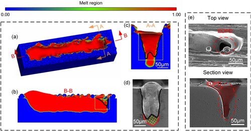
A noticeable depression is found at the trailing end of track in both simulation and experimental results in the case of laser power 340 W, as shown in Figure 3. The longitudinal cross-section morphology clearly shows a ‘V’ shaped depression, resembling a keyhole but on a smaller scale. While the transversal cross-section exhibits a ‘W’ shape, which accords well with the experimental cross-section. All these observations suggest that the developed model exhibits acceptable accuracy.

Figure 3. The melt track formation with laser power of 340 W and a scanning speed of 1.06 m/s. (a) Simulated 3D melt track. (b) Longitudinal cross-sectional view in the middle of simulated melt track. (c) Cross-sectional view of simulated melt track. (d) Cross-sectional view of the experimental melt track. (e) EOPD plots at another melt track with the same parameters.

3.2. Defect-process map

Based on the depression characteristics observed in the experiments, we propose a criterion to determine the occurrence of the EOPD defect. When the track end is significantly lower than the substrate, we will say the EOPD occurs under the current parameter set. In order to obtain EOPD-free parameter window, we perform numerous simulations with different laser powers and scanning speeds to correlate the process parameters with EOPD defect.

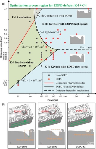
Figure 4(a) shows the defect-process map, showing the relationship between laser power, scanning speed and EOPD occurrence. The map is divided into five regions based on the melting mode and EOPD formation mechanisms. Conduction mode and the keyhole mode are two distinct melting modes in AM, defined based on the depth-to-width aspect ratio of the molten pool [40]. In the conduction mode, the input energy density is small and the molten pool is shallow. While in the keyhole mode, a critical cavity is formed in the front part of the molten pool, extending along the depth direction. These two modes are categorised based on volumetric energy density (VED), as specific in Equation (16) [41]. (16) $\mathrm{VED}={\displaystyle \frac{P}{\mathrm{VHD}}}$(16) where H (m) represents the layer thickness and D (m) signifies the diameter of laser beam. The energy density boundary for different melting modes is 2.5 × 10¹⁰ J/m³ for 316L [42]. It was first found that most of the EOPDs result from the keyhole shape and melt flow. When the molten metal does not completely fill this keyhole during the solidification process, a depression occurs at the end of the track. Therefore, a first threshold regarding the energy density of 7 × 10¹⁰ J/m³ has been established, below which the occurrence of EOPD is precluded even in the keyhole mode as shown in Figure 4(a) regions K-I and K-II. The specific EOPD defect formation process for this situation is illustrated in the flowing Section 3.3.1. However, with the increase in scanning speed, the occurrence of EOPD is not solely dependent on the energy density. Under high scanning speeds, the molten pool becomes longer and shallower, altering the shape of the keyhole. At this time, the solidification process plays the dominant role rather than the melt flow. The specific analysis of the mechanism change is discussed in detail in Section 3.3.2. Thus, a second boundary is developed based on the P–V relationship, as shown in Figure 4(a) region K-III. The curve boundary indicates that there are two thresholds for laser power and scanning speed which are 160 W and 1.1 m/s, respectively. Interestingly, this region K-III has a small overlap with the conduction mode region, indicating that the EOPD appears not only in the keyhole mode, but also in the conduction mode. The corresponding simulation result also confirms this guess. That is to say, keyhole is the main reason causing the EOPD but not the only reason. The specific analysis for EOPD in conduction mode is discussed in Section 3.3.3. Figure 4(b) shows the morphological characteristics of these three types of EOPD defects, respectively.

Figure 4. (a) In the P–V map, there are two distinct regions: a non-EOPD region (depicted in light green, comprising conduction and keyhole regimes) and an EOPD region (shown in light blue, including conduction, keyhole with EOPD in high-speed regime, and keyhole with EOPD in low-speed regime). The boundary between the EOPD and non-EOPD regions consists of a straight line with a VED of 7 × 10¹⁰ J/m³ and a curve determined by the equation ‘(V-1.1) (P-160)^0.7= 1.5’. Furthermore, the demarcation line between the keyhole and conduction regimes is represented by a straight line with a VED of 2.5 × 10¹⁰ J/m³. (b) Morphological characteristics of three types of EOPD defects.

3.3. EOPD formation mechanisms

3.3.1. EOPD occurs at low scanning speeds in keyhole mode

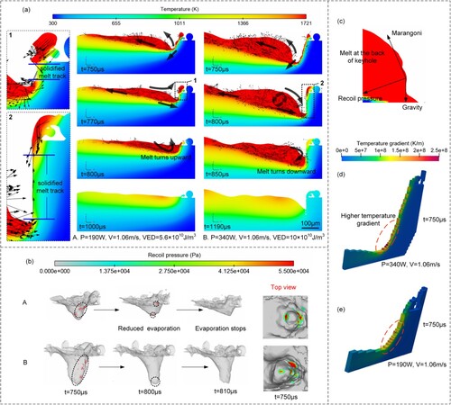
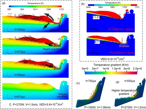
For the EOPD forming at low scanning speeds (slow than 1.1 m/s), two keyhole mode cases are compared to elucidate the mechanism of EOPD formation, with one of them exhibiting depression while the other is defect-free (see Figure 5). It can be seen case B with energy density of 10 × 10¹⁰ J/m³ has a much deeper keyhole than that in case A with energy density of 5.6 × 10¹⁰ J/m³. At 750 µs in both simulation cases, just after turning off the laser, the melt at the keyhole rear wall experiences steam recoil and Marangoni force, which overcomes the gravity effect and flow upward and backward (see Figure 5(a) and (c)). After 20 µs for case A or 50 µs for case B, the effect of recoil pressure dissipates since the evaporation phenomenon stops. At this time, melt behind the keyhole rear wall descends under the influence of gravity to fill the keyhole cavity. From this moment, the molten pool behaviours of two cases exhibit differences, leading to distinct outcomes in defect formation. It is worth noting that the low-energy density in case A results in a smaller temperature gradient at the front wall of the keyhole, reaching a maximum of approximately 2 × 10⁸ K/m, while the maximum temperature gradient at the front wall of the keyhole in case B is around 4.1 × 10⁸ K/m (see Figure 5(d, e)). Meanwhile, the keyhole in case A is much shallower than that in case B. Hence, the forward-flow melt below the keyhole tip in case A connects with the molten materials in the front of keyhole front wall and together forms a liquid channel when t = 770 µs. Upon contact with the descending melt from keyhole rear, this liquid channel leads to an upward flow of the combined melt, resulting in the formation of a counterclockwise flow pattern and filling the keyhole cavity quickly, as illustrated in Figure 5(a) t = 800 µs. On the contrary, larger temperature gradient, longer cooling time (50 µs) and deeper keyhole in case B promotes the melt in front of keyhole to solidify. The forward flow of melt below the keyhole tip is then suppressed, suggesting the upward-flow liquid channel cannot form. Consequently, when filling the keyhole to a certain extent, the melt behind the keyhole flows downward to establish a clockwise flow pattern as shown in Figure 5(a) t = 850 µs. This flow behaviour cannot fill the keyhole cavity in time and finally leave a depression after solidification. In summary, the extended vapour recoil associated with high-energy density and the significant temperature gradient in front of the keyhole contribute to the increased likelihood of depression formation at the end of the melt track.

Figure 5. Simulation of the molten pool under low-speed scanning (1.06 m/s). (a) Sequential solidification of the molten pool at the end of the melt track for laser powers of 190 and 340 W, respectively. (b) Recoil pressure on the molten pool at the keyhole for laser powers of 190 and 340 W, respectively. (c) The force diagram of the melt at the back of the keyhole at t = 750 µs in case B. (d) Temperature gradient at the solid–liquid interface of the molten pool at the moment the laser is deactivated in case A. (e) Temperature gradient at the solid–liquid interface of the molten pool at the moment the laser is deactivated in case B.

3.3.2. EOPD occurs at high scanning speeds in the keyhole mode

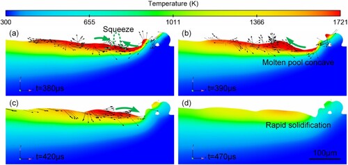
In the P–V diagram, a EOPD defect occurs even when the energy density is lower than 7 × 10¹⁰ J/m³, once the high scanning speed demarcation line is surpassed. A simulation case with a scanning speed of 1.5 m/s and VED of 5.6 × 10¹⁰ J/m³ has been chosen to compare with case A with same VED for analysing the second way of EOPD formation. Likewise, at t = 550 µs, after turning off the laser, the molten pool experiences steam recoil and Marangoni force. Its flow pattern resembles that of the 190 W, 1.06 m/s molten pool (Figure 6(a)). The molten materials behind the keyhole are unable to flow forward to fill the keyhole immediately until 20 µs later. However, it is found that the filling behaviour just maintains less than another 20 µs as shown in Figure 6(a) t = 590 µs, since the melt below keyhole tip has already solidified, which is different from that in case A. To discover the reason why the melt below keyhole tip solidifies in such a short time frame, the temperature gradients and solidification rates for the corresponding regions in case A and case C are calculated and compared. Figure 6(c) and (d) shows the calculated temperature gradients in case A and case C, respectively. It is clear that the target region in case C has a higher temperature gradient value (2 × 10⁸ K/m vs. 2.5 × 10⁸ K/m) and a larger high temperature gradient area than those in case A. The average solidification rate of the target region is used for comparison. The specific equation [43] is given in Equation (17). (17) $v_s=V\times \sin \theta$(17) where v_s (m/s) denotes the solidification rate and θ signifies the acute angle between the tangent vector of solidification front and the scanning direction, which is measured and shown in Figure 6(b). Thus, the calculated solidification rates for case A and case C are 0.2 and 0.25 m/s, respectively. Moreover, it is seen from Figure 6(b) that both the molten pool and the keyhole are elongated in the scanning direction in case C due to the high scanning speed. Therefore, the heat dissipation from the molten pool to air is more significant in the target region of case C, since the area of the target region is larger. In general, the melt below keyhole tip in case C can solidify rapidly due to higher temperature gradient, larger solidification rate and more significant heat dissipation from heat to air. Then, the fast solidification presents a remarkable flow resistance, preventing the molten material filling the cavity and finally inducing an EOPD defect.

Figure 6. Simulation of the molten pool under high-speed scanning. (a) Sequential solidification diagram of the molten pool at a VED of 5.6 × 10¹⁰ J/m³ and a scanning speed of 1.5 m/s. (b) Solid–liquid interface diagram of the molten pool at the same VED but with scanning speeds of 1.06 and 1.5 m/s, respectively, at the moment the laser is deactivated. (c) Temperature gradient at the solid–liquid interface of the molten pool at the moment the laser is deactivated in case A. (d) Temperature gradient at the solid–liquid interface of the molten pool at the moment the laser is deactivated in case C.

3.3.3. EOPD occurs in conduction mode

It implies that even though the molten pool is in conduction mode, high scanning speed may result in a slight depression at the end of track. In conduction mode, there is no melt evaporation to create keyholes, but the Marangoni force does lead to the formation of a concave surface at the front of the molten pool. When the laser is turned off at t = 380 µs, the surface melt at the front of the molten pool flows backward due to the Marangoni force. After 10 µs, the melt accumulates behind the concave surface, as shown in Figure 7(b). The temperature decreases gradually, causing the surface temperature gradient declines and the Marangoni effect weakens. At t = 420 µs, the accumulated surface melt begins to flow forward to fill the cavity in the front under the influence of gravity. However, at high scanning speeds, the molten pool can solidify rapidly, preventing the complete filling of the concave surface. This incomplete filling finally gives rise to the formation of a harmless or less harmful EOPD.

Figure 7. Sequence of solidification of the molten pool at the end of the melt track at laser powers of 170 W and a scanning speed of 2.1 m/s (conduction mode).

4. EOPD reduction method

The conduction mode EOPDs have a narrow process parameter window and have a weak negative effect on the overall LPBF process as mentioned before. Therefore, it is not necessary to develop a specific method to reduce this kind of depression. To reduce the formation frequency of severe EOPDs, we do recommend low speed (slower than 1.1 m/s) scanning strategy to avoid the high-speed type EOPDs. Hence, in this study, we mainly focus on the reduction method of addressing EOPDs which occur at low scanning speeds. Based on the EOPD formation mechanism 1, we decrease the laser power to decrease the input VED at the end of the track where the depression appears. This optimisation approach targets the depression defect without impacting the overall laser power during printing. There are numerous strategies for adjusting the power, and it's crucial to take the equipment's conditions into account when selecting the most appropriate strategy. Therefore, in conjunction with the experimental equipment conditions, this section primarily focuses on two strategies for power adjustment: the ‘step’ and ‘gradual’ approaches.

4.1. ‘Step’ variable power strategy

The ‘step’ variable power strategy is characterised by having only one power change point, where the power is reduced directly to the target power. Since there is only one power change point, this strategy allows for scanning from the power change point to the end of the melt track.

As shown in Figure 8(a), the applied laser power is 340 W and a narrow and deep (depth 132 µm) EOPD shows at the end of track. The ‘step’ variable power strategy is employed to mitigate this deep EOPD by reducing to 190 W when 500 µm away from the end point. Figure 8(c) shows the longitudinal cross-section of the experimental track created using the ‘step’ variable power strategy. It can be observed that an EOPD, with a depth of approximately 31 µm, forms at the end of the track, representing an improvement compared to the EOPD observed with constant power. Additionally, no depression forms at the point of power change. Figure 8(d) presents a longitudinal cross-section of a simulated melt track created using the same strategy, which, like the experimental results, also results in a depression at the end of the track with a depth of approximately 32 µm.

Figure 8. Comparative illustration of variable power printing strategy versus constant power printing: experimental and simulation. Longitudinal cross-sectional views of the (a) experimental and (b) simulated melt tracks with laser power maintained at 340 W. Longitudinal cross-sectional views of the (c) experimental and (d) simulated melt tracks using the ‘step’ variable power method. Longitudinal cross-sectional views of the (e) experimental and (f) simulated melt tracks using the ‘gradual’ variable power method. (g) Top view of the experimental melt track with the ‘step’ variable power method. (h) Top view of the experimental melt track using the ‘gradual’ variable power method.

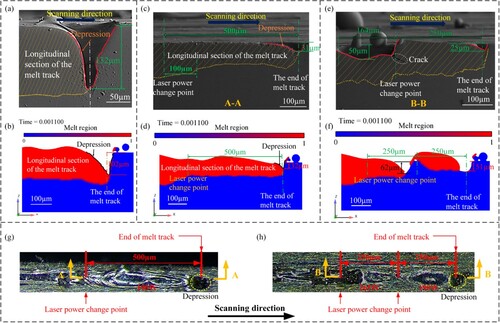
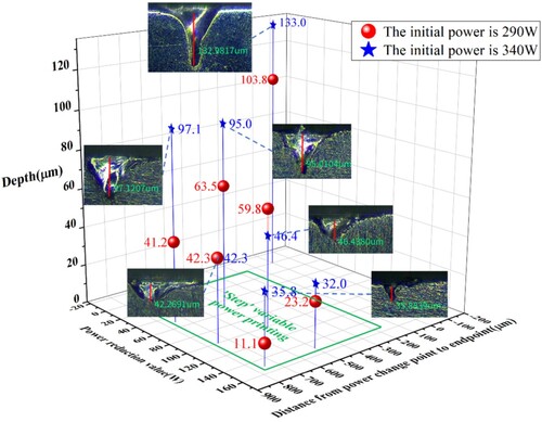
Figure 9 presents the statistical analysis of the outcomes when printing a single track using the ‘step’ variable power strategy. In this context, ‘depth’ signifies the measurement from the bottom of the depression to the top surface of the substrate. The graph illustrates significant deviations on EOPD depths at the end of the fusion track when varying both power change values and positions. A greater power reduction leads to a more powerful EOPD reduction effect, e.g. the EOPD depth of 35 µm after using power reduction of 150 W, approximately 75% shallower than that observed in the case using constant power. It’s worth noting that the distance from the power change position to the end point has a relatively weak effect on depression depth reduction. However, this step distance for different initial laser power and power reduction should not be too short, as this may lead to the decline of EOPD reduction effect. As shown in Figure 8(c), the depth of the molten pool spans about 100 µm to achieve stable when laser power decreases. In this case, the step distance should not be smaller than this 100 µm threshold. In summary, the ‘step’ variable power strategy can effectively mitigate the EOPD defect without introducing other post-process method.

Figure 9. Statistical chart of EOPD phenomena in melt tracks printed using the ‘step’ variable power method with different power change values and positions of power change points.

4.2. ‘Gradual’ variable power strategy

The ‘gradual’ variable power strategy is characterised by a gradual reduction in laser power. After each reduction in laser power, there is a scanning distance during which the laser power remains a constant value until reaching the next power change point. However, since the total length of the variable power printing melt track cannot be too long, the length of each step should be limited.

Figure 8(d) illustrates an as-built track using ‘gradual’ variable power strategy, featuring two power reduction points and each step distance of 250 µm. The laser power is decreased by 75 W each time, resulting in a total reduction of 150 W. Figure 8(g) displays a longitudinal cross-section, revealing the formation of an EOPD with a depth of approximately 25 µm. This represents a significant improvement in EOPD reduction compared to that observed under constant power condition. However, near the second power change point, a depression with a width of approximately 164 µm and a depth of about 50 µm forms, which is also detrimental to the fusion track. To elucidate why the depression emerges near the second power change point, a simulation corresponding to the ‘gradual’ variable power strategy is conducted. We have considered the laser oscillation issue due to the instrument limitation in on-line laser power modification where the laser does not come out while the mirror is still in motion. Hence, introducing an additional step without energy input following the power change point. The simulation result, depicted in Figure 8(f), exhibits a depression at the second power change point. As the laser scans through the first power change point, the melt track lacks subsequent energy input due to a brief period of no laser. This situation is similar to the end of the melt track described earlier where the previous melted materials cannot fill the keyhole completely, and an EOPD-like phenomenon is formed in the middle of the melt track. At the same time, the mirrors are still moving according to a predetermined trajectory during the period of laser non-emission, so that the laser is emitted again after a small distance away from the first power change point. Then, the newly melted materials are driven back by the Marangoni force to fill the previous depression. However, this flow aggravates the depression occurring at the second power change point. The subsequent molten pool flow after laser oscillation cannot completely eliminate this defect. Consequently, a depression shows in the middle of track near the second power. Because of the device limitation, the new defects caused by the ‘gradual’ power change strategy are difficult to avoid. Therefore, the ‘step’ variable power strategy is better than the ‘gradual’ power change strategy in optimising the EOPD phenomenon.

5. Conclusion

In this paper, the following conclusions are drawn from mesoscopic simulations of the LPBF process and the corresponding experimental results.

1. A defect-process map is developed based on our observations of EOPD phenomena under different process parameters. It clearly distinguishes areas with depressions from those without depressions. EOPD defect occurs in the melt track when VED exceeds 7 × 10¹⁰ J/m³ at low scanning speeds (V < 1.1 m/s), and also occurs in the melt track when (V-1.1) (P-160)^0.7> 1.5 at high scanning speeds (V > 1.1 m/s). The region with keyhole phenomenon while without depression phenomenon is also specifically indicated to provide guidance for subsequent research work.

2. Three types of EOPD formation mechanisms are found based on the simulation results. In keyhole mode, two scenarios arise: at low scanning speeds, the extended vapour recoil force and the higher temperature gradient at the leading edge of the keyhole facilitate the formation of EOPDs at the melt track. At higher scanning speeds, the shallower molten pool morphology and increased solidification rate lead to the rapid transformation of the keyhole into EOPDs. In the conduction mode, EOPDs formed by the Marangoni force, along with a faster solidification rate.

3. An improvement is proposed to address EOPDs occurring at low scanning speeds by using variable laser powers during printing. Corresponding experiments and simulations prove the feasibility and effectiveness of the ‘step’ variable power strategy on reducing the depth of EOPD.

Disclosure statement

No potential conflict of interest was reported by the author(s).

Data availability statement

The data that support the findings of this study are available from the corresponding author upon reasonable request.

Additional information

Funding

This work was supported in part by the National Natural Science Foundation of China [grant number 52175481].

References

- Zhang C, Li Z, Zhang J, et al. Additive manufacturing of magnesium matrix composites: comprehensive review of recent progress and research perspectives. J Mag Alloys. 2023. doi:10.1016/j.jma.2023.02.005
- Webster S, Lin H, Carter III FM, et al. Physical mechanisms in hybrid additive manufacturing: a process design framework. J Mater Process Technol. 2022;291:117048. doi:10.1016/j.jmatprotec.2021.117048
- Wang S, Ning J, Zhu L, et al. Role of porosity defects in metal 3D printing: formation mechanisms, impacts on properties and mitigation strategies. Mater Today. 2022. doi:10.1016/j.mattod.2022.08.014
- Wei C, Li L. Recent progress and scientific challenges in multi-material additive manufacturing via laser-based powder bed fusion. Virtual Phys Prototyp. 2021;16(3):347–371. doi:10.1080/17452759.2021.1928520
- Lin X, Wang Q, Fuh JYH, et al. Motion feature based melt pool monitoring for selective laser melting process. J Mater Process Technol. 2022;303:117523. doi:10.1016/j.jmatprotec.2022.117523
- Gockel J, Sheridan L, Koerper B, et al. The influence of additive manufacturing processing parameters on surface roughness and fatigue life. Int J Fatigue. 2019;124:380–388. doi:10.1016/j.ijfatigue.2019.03.025
- Nicoletto G. Influence of rough as-built surfaces on smooth and notched fatigue behavior of L-PBF AlSi10Mg. Addit Manuf. 2020;34:101251. doi:10.1016/j.addma.2020.101251
- Spece H, Yu T, Law AW, et al. 3D printed porous PEEK created via fused filament fabrication for osteoconductive orthopaedic surfaces. J Mech Behav Biomed Mater. 2020;109:103850. doi:10.1115/1.0004270v
- Andrukhov O, Huber R, Shi B, et al. Proliferation, behavior, and differentiation of osteoblasts on surfaces of different microroughness. Dent Mater. 2016;32(11):1374–1384. doi:10.1016/j.dental.2016.08.217
- Dai N, Zhang LC, Zhang J, et al. Corrosion behavior of selective laser melted Ti-6Al-4 V alloy in NaCl solution. Corros Sci. 2016;102:484–489. doi:10.1016/j.corsci.2015.10.041
- Li EL, Wang L, Yu AB, et al. A three-phase model for simulation of heat transfer and melt pool behaviour in laser powder bed fusion process. Powder Technol. 2021;381:298–312. doi:10.1016/j.powtec.2020.11.061
- Liao B, Xia RF, Li W, et al. 3D-printed ti6al4v scaffolds with graded triply periodic minimal surface structure for bone tissue engineering. J Mater Eng Perform. 2021;30:4993–5004. doi:10.1007/s11665-021-05580-z
- Li E, Zhou Z, Wang L, et al. Melt pool dynamics and pores formation in multi-track studies in laser powder bed fusion process. Powder Technol. 2022;405:117533. doi:10.1016/j.powtec.2022.117533
- Guo L, Geng S, Gao X, et al. Numerical simulation of heat transfer and fluid flow during nanosecond pulsed laser processing of Fe78Si9B13 amorphous alloys. Int J Heat Mass Transfer. 2021;170:121003. doi:10.1016/j.ijheatmasstransfer.2021.121003
- Guo L, Li Y, Geng S, et al. Numerical and experimental analysis for morphology evolution of 6061 aluminum alloy during nanosecond pulsed laser cleaning. Surf Coat Technol. 2022;432:128056. doi:10.1016/j.surfcoat.2021.128056
- Li S, Liu D, Mi H, et al. Numerical simulation on evolution process of molten pool and solidification characteristics of melt track in selective laser melting of ceramic powder. Ceram Int. 2022;48(13):18302–18315. doi:10.1016/j.ceramint.2022.03.089
- Aboulkhair NT, Maskery I, Tuck C, et al. On the formation of AlSi10Mg single tracks and layers in selective laser melting: microstructure and nano-mechanical properties. J Mater Process Technol. 2016;230:88–98. doi:10.1016/j.jmatprotec.2015.11.016
- Thijs L, Kempen K, Kruth JP, et al. Fine-structured aluminium products with controllable texture by selective laser melting of pre-alloyed AlSi10Mg powder. Acta Mater. 2013;61(5):1809–1819. doi:10.1016/j.actamat.2012.11.052
- Qiu C, Adkins NJE, Attallah MM. Microstructure and tensile properties of selectively laser-melted and of HIPed laser-melted Ti–6Al–4 V. Mater Sci Eng A. 2013;578:230–239. doi:10.1016/j.msea.2013.04.099
- Kazemi Z, Soleimani M, Rokhgireh H, et al. Melting pool simulation of 316L samples manufactured by selective laser melting method, comparison with experimental results. Int J Therm Sci. 2022;176:107538. doi:10.1016/j.ijthermalsci.2022.107538
- Cao L. Workpiece-scale numerical simulations of SLM molten pool dynamic behavior of 316L stainless steel. Comput Math Appl. 2021;96:209–228. doi:10.1016/j.camwa.2020.04.020
- Liu B, Fang G, Lei L, et al. Predicting the porosity defects in selective laser melting (SLM) by molten pool geometry. Int J Mech Sci. 2022;228:107478. doi:10.1016/j.ijmecsci.2022.107478
- Ur Rehman A, Pitir F, Salamci MU. Full-field mapping and flow quantification of melt pool dynamics in laser powder bed fusion of SS316L. Materials. 2021;14(21):6264. doi:10.3390/ma14216264
- Chia HY, Wang L, Yan W. Influence of oxygen content on melt pool dynamics in metal additive manufacturing: high-fidelity modeling with experimental validation. Acta Mater. 2023;249:118824. doi:10.1016/j.actamat.2023.118824
- Cheng B, Loeber L, Willeck H, et al. Computational investigation of melt pool process dynamics and pore formation in laser powder bed fusion. J Mater Eng Perform. 2019;28:6565–6578. doi:10.1007/s11665-019-04435-y
- Li X, Guo Q, Chen L, et al. Quantitative investigation of gas flow, powder-gas interaction, and powder behavior under different ambient pressure levels in laser powder bed fusion. Int J Mach Tools Manuf. 2021;170:103797. doi:10.1016/j.ijmachtools.2021.103797
- Wu Y, Li M, Wang J, et al. Powder-bed-fusion additive manufacturing of molybdenum: process simulation, optimization, and property prediction. Addit Manuf. 2022;58:103069. doi:10.1016/j.addma.2022.103069
- Wu S, Yang Y, Huang Y, et al. Study on powder particle behavior in powder spreading with discrete element method and its critical implications for binder jetting additive manufacturing processes. Virtual Phys Prototyp. 2023;18(1):e2158877. doi:10.1080/17452759.2022.2158877
- Klassen A, Schakowsky T, Kerner C. Evaporation model for beam based additive manufacturing using free surface lattice Boltzmann methods. J Phys D Appl Phys. 2014;47(27):275303. doi:10.1088/0022-3727/47/27/275303
- Cao L. Mesoscopic-scale numerical simulation including the influence of process parameters on slm single-layer multi-pass formation. Metall Mater Trans A. 2020;51:4130–4145. doi:10.1007/s11661-020-05831-z
- Zhuang JR, Lee YT, Hsieh WH, et al. Determination of melt pool dimensions using DOE-FEM and RSM with process window during SLM of Ti6Al4V powder. Opt Laser Technol. 2018;103:59–76. doi:10.1016/j.optlastec.2018.01.013
- Li Y, Gu D. Thermal behavior during selective laser melting of commercially pure titanium powder: numerical simulation and experimental study. Addit Manuf. 2014;1–4:99–109. doi:10.1016/j.addma.2014.09.001
- Dai D, Gu D. Thermal behavior and densification mechanism during selective laser melting of copper matrix composites: simulation and experiments. Mater Des. 2014;55(0):482–491. doi:10.1016/j.matdes.2013.10.006
- Wang S, Zhu L, Dun Y, et al. Multi-physics modeling of direct energy deposition process of thin-walled structures: defect analysis. Comput Mech. 2021;67:c1229–c1242. doi:10.1007/s00466-021-01992-9
- Wu J, Zheng J, Zhou H, et al. Molten pool behavior and its mechanism during selective laser melting of polyamide 6 powder: single track simulation and experiments. Mater Res Express. 2019;6. doi:10.1088/2053-1591/ab2747
- Cho JH, Farson DF, Milewski JO, et al. Weld pool flows during initial stages of keyhole formation in laser welding. J Phys D Appl Phys. 2009;42. doi:10.1088/0022-3727/42/17/175502
- Sinha KN. Identification of a suitable volumetric heat source for modelling of selective laser melting of Ti6Al4V powder using numerical and experimental validation approach. Int J Adv Manuf Technol. 2018;99:2257–2270. doi:10.1007/s00170-018-2631-4
- Fu CH, Guo YB. Three-dimensional temperature gradient mechanism in selective laser melting of Ti-6Al-4V. J Manuf Sci Eng. 2014;136(6):061004. doi:10.1115/1.4028539
- Ansari P, Rehman AU, Pitir F, et al. Selective laser melting of 316 l austenitic stainless steel: detailed process understanding using multiphysics simulation and experimentation. Metals. 2021;11(7):1076. doi:10.3390/met11071076
- Zhao C, Shi B, Chen S, et al. Laser melting modes in metal powder bed fusion additive manufacturing. Rev Mod Phys. 2022;94(4):045002. doi:10.1103/revmodphys.94.045002
- Bertoli US, Wolfer AJ, Matthews MJ, et al. On the limitations of volumetric energy density as a design parameter for selective laser melting. Mater Des. 2017;113:331–340. doi:10.1016/j.matdes.2016.10.037
- Dash A, Kamaraj A. Prediction of the shift in melting mode during additive manufacturing of 316L stainless steel. Mater Today Commun. 2023: 107238. doi:10.1016/j.mtcomm.2023.107238
- Majeed M, Khan HM, Rasheed I. Finite element analysis of melt pool thermal characteristics with passing laser in SLM process. Optik. 2019;194:163068. doi:10.1016/j.ijleo.2019.163068