A novel design strategy to enhance buckling resistance of thin-walled single-cell lattice structures via topology optimisation

ABSTRACT

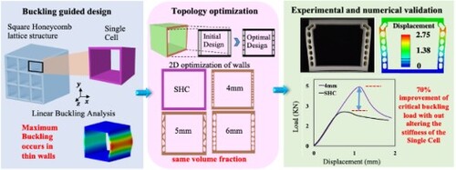
Lattice structures with thin walls or members are susceptible to instability due to their limited buckling strength. We propose a design methodology that utilises topology optimisation techniques to create lattice structure members with improved buckling resistance, demonstrated here on a single cell of a thin-walled square honeycomb lattice. We utilise the buckling mode of the single cell as a reference to inform the design of modified lattice structure members via optimisation, while ensuring the weight and stiffness of the structure remain unchanged. We apply a 2D topology optimisation method with the objective of maximising buckling load factors, while simultaneously enforcing constraints on stiffness and volume fraction within the optimisation domain. A family of designs is created via a parametric study, considering optimisation parameters like the thickness of the buckling member and the active domain. Designing and fabricating these structures also consider additive manufacturing constraints, such as minimal feature size and overhang. Experimental analysis of fabricated structures reveals a remarkable 70% increase in buckling strength without altering stiffness or weight. Numerical simulations corroborate these findings, with a discrepancy of less than 10%. This methodology shows the potential to enhance buckling resistance of thin-walled lattices in various lattice types while maintaining base cell stiffness.

GRAPHICAL ABSTRACT

KEYWORDS:

• Square honeycomb
• lattice structure buckling
• topology optimisation
• finite element analysis
• additive manufacturing

Nomenclature

Abbreviations
LS	=	lattice structure
SHC	=	square honeycomb
TO	=	topology optimisation
FE	=	finite element
SC	=	single cell
SIMP	=	Solid Isotropic Material with Penalisation
BLF	=	buckling load factor
BC	=	boundary condition
AM	=	additive manufacturing
DFAM	=	design for AM
CAD	=	computer-aided design
STL	=	stereo lithography
FDM	=	fusion deposition modelling

Notations

Variables
${\mathrm{\Omega }}_h$	=	Structure design domain
m	=	number of FEs
${\mathrm{\Omega }}_e$	=	element domain
n	=	total dofs
${\rho }_e$	=	pseudo density
$\widehat{{\rho }_e}$	=	filtered element density
$\eta$,$\beta$	=	projection parameters
rmin	=	density filter
$p_K$	=	penalisation factor for stiffness
$p_G$	=	penalisation factor for stress
EK	=	SIMP interpolation of Young’s modulus for stiffness matrix
EG	=	SIMP interpolation of Young’s modulus for stress matrix
$E_{\min }$	=	void element Young’s modulus
$E_s$	=	solid element Young’s modulus
A	=	active domain region
P1	=	passive domain region with 1 density
P0	=	passive domain region with 0 density
$V$	=	total volume fraction
$c$	=	compliance
${\lambda }_1$	=	fundamental BLF
$\mu$	=	Eigen value
$J^{\mathrm{KS}}$	=	aggregation function
$p_{\mathrm{AGG}}$	=	aggregation parameter
$J_0^{\mathrm{KS}}$	=	aggregation function for ${\mu }_1$
$J_1^{\mathrm{KS}}$	=	aggregation function for constraints
$\mathrm{gv},\mathrm{gc}$	=	constraints on volume fraction, compliance
$\overline{\lambda }$	=	minimum prescribed BLF
${\delta }_{\mathit{e}A}$	=	dirac delta
$V_f,c_f$	=	maximum allowed volume fraction, compliance

Vectors
$\mathit{\rho }$	=	pseudo densities
${\mathit{\rho }}_A$	=	active pseudo densities
${\mathit{\rho }}_{P1}$	=	passive pseudo densities vector 1
${\mathit{\rho }}_{P0}$	=	passive pseudo densities vector 0
F	=	load vector
u	=	displacement vector
$\mathit{v}$	=	eigen vector
$\mathit{\phi }$	=	normalised Eigen vector
${\mathit{w}}_i$	=	adjoint vector

Sets
${\mathbb{R}}^n$	=	n tuple

Matrices
K	=	linear stiffness matrix
G	=	stress stiffness matrix

Subscripts
KS	=	Kreisselmeier and Steinhauser
e	=	element
s	=	solid

Pseudo code variables
nelx, nely	=	FE mesh size
penalK	=	penalisation factor for stiffness
penalG	=	penalisation factor for stress
rmin	=	density filter radius
ft	=	projection filtering scheme with
beta,eta	=	projection parameters
ftBC	=	filter BCs, Neumann or Dirichlect
ocPar	=	optimality criteria parameters
maxit	=	maximum number of iterations
Lx	=	the physical length of the domain
nEig	=	number of BLFs in optimisation
pAgg	=	initial value of KS aggregation factor
prSel	=	data structure specifying optimisation problem
Cmax/C0	=	ratio of maximum allowable compliance to initial compliance
start,maxP,ds,dP	=	continuation parameters

1. Introduction

Lightweight structural design is frequently of paramount importance in engineering, particularly within aerospace and space applications. Lattice structures (LSs), formed through the arrangement of beams, struts, or plates, are extensively used due to their excellent stiffness-to-weight ratio, superior energy absorption capabilities, and specialised acoustic attributes [1]. Recent advancements in additive manufacturing (AM) technologies, which offer design freedom, enable the fabrication of LSs with exceptionally thin members, thereby precipitating both a reduction in weight and an increase in stiffness [2]. The presence of slender beams/struts/plates can introduce instability in LSs, leading to buckling failure under compressive loads, which in turn reduces the structure's load-carrying capacity [3]. Therefore, buckling is a critical design factor to prevent sudden failure, often occurring before the material reaches its yield stress. In LSs, composed of unit cells, buckling can occur either locally in individual unit cell members or globally in the entire LS, with the former being more likely [3]. It is therefore crucial to devise strategies that boost the unit cell’s buckling resistance, thus enhancing the overall buckling performance of the LS.

Numerous researchers endeavoured to enhance the buckling response of LSs [4–6] and utilised buckling to induce desirable properties, such as an auxetic response [7]. However, this is often achieved by modifying the stiffness and relative density of the LS, which can compromise its lightweight characteristics. Recently, the authors demonstrated that, guided by the buckling modes of a LS, it is possible to enhance the buckling resistance of the lattice unit cell, without changing its stiffness and volume fraction [8]. However, in this earlier study, the weak regions of the LS were altered using conventional shapes like hollow rectangles, hollow hexagons, and angles. These modifications demonstrated an increase in buckling strength of up to 35% without compromising the structure's stiffness. Therefore, there is a requirement to utilise more systematic optimisation methods to design members that provide the highest possible buckling resistance [9,10].

Topology optimisation (TO) identifies optimal structural configurations within a specified design domain, considering multiple constraints. Buckling-driven TO regained prominence in recent years, particularly as TO applications extend to complex structures comprised of lattices or plates. The pioneering work of Neves et al. [10] involved the development of a TO model aimed at controlling the critical buckling load of slender rod structures, ultimately maximising the linearised buckling load. Subsequently, several TO studies, focusing on both buckling constraints and the maximisation of buckling load were reported. Mitjana et al. [11] developed a topological gradient-based algorithm for minimising structural mass while adhering to stress and buckling constraints. Gao et al. [12,13] proposed an automatic parameter adjustment strategy within the Solid Isotropic Material with Penalisation (SIMP) framework to account for buckling constraints in the TO process, optimising material layout. Geometric nonlinearity problems optimised continuum structures against buckling in studies [14–16] and large eigenvalue problems were also studied [17]. TO based on evolutionary structural optimisation for problems with buckling constraints is also available in the literature [18]. Using topology optimisation for microstructure buckling strength optimisation was first studied by Neves et al. [19] which focused on cell-periodic buckling modes. Thomsen et al. [20] proposed a TO framework targeting the initial design of microscopic buckling instabilities in periodic materials, with the goal of achieving periodic cellular materials with maximum strength. 2D and 3D material microstructures were also designed to enhance buckling strength based on linear material analysis [21,22]. Compared to studies that treat buckling as a constraint in a stiffness design problem, research focusing on buckling load as the objective function is limited. Noteworthy contributions include works by Lindgaard and Lund [23], Lindgaard et al. [24], Luo and Tong [25], Wang and Sigmund [26], and others. Additionally, Ferrari and Sigmund [27] offered a multilevel large-scale TO approach with MATLAB codes for two scenarios: one focused on maximising buckling load while constraining compliance and volume fraction, and the other aimed at minimising volume fraction (weight) while constraining buckling load and compliance. In the current study, where the objective is to maintain the same stiffness of the structure without altering the overall volume fraction, the TO approach of maximising buckling load factors (BLFs) while imposing constraints on compliance and volume fraction appears most suitable.

Once the TO designs are obtained, fabricating them for experimental testing is the next step. Design for Additive Manufacturing (DFAM) enables design opportunities utilising the unique capabilities of AM technologies, including shape, hierarchical, functional, and material complexities [28]. The layer-by-layer AM fabrication helps in fabricating complex features such as thin features, channels, or overhangs that are essential parts of a TO design arising from low parameter values of filter radius and penalisation constants. However, there are various AM constraints, such as the need for support structures and their removal, minimum printable feature size, and overhang size, to name a few [29]. These constraints vary depending on the type of printer and the printing method. For example, a printer based on SLA technology in reference [30] exhibited a minimum feature size of 0.2 mm, while for FDM, depending on the nozzle size, the minimum feature size is 0.8 mm, which further changes depending on the capabilities of the printer. Reducing the lattice cell size during part-level design will further decrease various feature sizes. Therefore, the cell size should be chosen to ensure printability, with the minimum feature size falling well within allowable limits. To facilitate printing, minor redesign of the obtained TO designs may be necessary, which can be effortlessly performed in any computer-aided design/manufacturing (CAD/CAM) software without altering any mechanical properties achieved by TO, such as volume fraction, compliance, or buckling resistance. The redesign process involves several iterations of computational simulations on these CAD designs, guided by the AM constraints, before obtaining the final design that will be fabricated.

Apart from this, from a manufacturing point of view, there can be process-related defects within complex geometrical features designed by TO [31]. This is because TO is a purely geometrical design tool and rarely accounts for process constraints and conditions. Geometry design by TO and manufacturing simulations are viewed as two separate realms, while recently attempts are made to combine the two under a holistic computational design tool by incorporating process models as additional constraints in TO [32].

This paper introduces a novel methodology for implementing buckling load maximisation in a single-cell (SC) structure using a 2D TO approach tailored for lattices. Here, we implement this methodology in thin-walled square honeycomb (SHC) LSs, using the buckling mode of the SHC SC as a reference to guide TO. The optimisation's objective function is the maximisation of BLFs, aimed at enhancing the structure's buckling resistance. The optimisation constraints include compliance (stiffness) and volume fraction, thus ensuring the preservation of both the UC's stiffness and volume fraction. We generated a range of designs through a parametric investigation, varying optimisation parameters such as filter radius and maximum compliance limit along with geometry parameters such as the thickness of the buckling member and the optimisation's active domain. The research focused on assessing the compressive buckling strength of additively optimised LSs, and this evaluation was validated through the implementation of finite element (FE) modelling techniques.

The proposed method is specifically applied to single-cell of the thin-walled lattice structures, such as square honeycomb, commonly used as stiffeners in aerospace vehicles. These thin-walled structures are capable of resisting in-plane buckling loads. Hence, these structures can undergo 2D topology optimisation to achieve a buckling-resistant optimal design. The methodology is equally applicable to any 2D lattice structure, provided that we can identify the buckling modes, select the active domain around these modes, and aim to achieve the best-optimised design resistant to buckling. While the study primarily investigates a single-cell structure, the results’ applicability to scenarios involving multi-cell or entire structures can be achieved by adjusting the boundary conditions to accommodate a multi-cell lattice and scaling the methodology outlined in this paper to three-dimensional topology optimisation (3D TO). Consequently, the paper concludes with a discussion on the scalability of the optimisation approach and its implications for larger structures.

2. Methodology

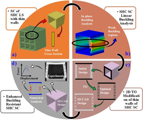
In this section, we present our innovative design methodology for achieving topology-optimised buckling-resistant lattice SCs, as depicted in Figure 1. The LS chosen involved 3D SHC with a series of square-shaped cells arranged in a honeycomb pattern, forming a grid-like structure with thin walls or partitions between adjacent cells. The initial design is a SC of this SHC structure, which is one square cell with thin walls (Figure 1(a)). The objective is to optimise the thin wall geometry of the SC using TO, to enhance its in-plane buckling resistance, while adhering to compliance (stiffness) constraints and maintaining the volume fraction constant. To achieve this, we perform a numerical 3D linear buckling analysis on a SHC SC under compressive loading using the ABAQUS FE software. It is to be noted here that this work deals with buckling analysis of the SC as an independent structure and not a part of a LS, hence periodic boundary conditions (BCs) are not imposed. The term SC is used to refer to the fact that structure geometry is inspired from a unit cell of a LS, but without periodicity conditions it is not representative of the LS, instead a stand-alone square cell structure. Analyzing prominent buckling regions in the mode shapes from this analysis helps identify the members most susceptible to buckling, with vertical walls often exhibiting buckling in a 3D-SHC SC under compressive loads (Figure 1(b)). Consequently, we modify these lattice columns by employing buckling-based TO, whilst maintaining a constant relative density of the SC. To enhance the buckling resistance of the buckled walls, we utilised 2D-SHC SC as the design domain (as shown in Figure 1(c)) and employed TO codes available in the literature [27]. The 2D-SHC SC lattice is divided into distinct regions: active, passive, and void, within the design domain as shown by grey, black and transparent regions, respectively, on the initial design in Figure 1(c). Throughout the optimisation process, only the active regions undergo material evolution, whereas the passive regions retain a consistent solid material state, and the void regions remain unchanged. The areas identified as the most vulnerable to buckling represent the active regions, while the remaining parts of the lattice face remain passive in this study. We explore three different combinations of active–passive region configurations in this work and analyse the resulting 2D geometry that emerges after TO in each case. After obtaining the optimal wall lattice design, it is extruded into the third dimension to create the 3D SC. This newly generated 3D-SHC SC is then manufactured for experimental analysis and is subsequently validated through numerical simulations, including post-buckling analyses conducted in ABAQUS (Figure 1(d)).

Figure 1. A TO-driven approach to design buckling-resistant LSs.

3. Buckling-based 2D TO

In this study, we employed 2D TO for designing the buckling-resistant SHC LSs. We followed the methodology outlined by Ferrari et al. [27], who developed a 250-line MATLAB program for optimising linearised buckling. Within this MATLAB code, the BLFs of a structure are treated either as the objective function or as constraints, leading to a significantly more efficient and computationally robust improvement compared to their previous code [33]. Initially, we reduce TO process for the 3D SHC lattice to a 2D problem. This entails optimising a 2D SHC SC and subsequently applying the obtained optimal 2D topology to the entire lattice effectively. This dimension reduction accelerates the optimisation process significantly without compromising the primary objective of achieving maximum buckling resistance. Next, the theory underpinning the buckling-based TO process on a 2D design domain is briefly described.

3.1. Formulations

Consider the 2D design domain ${\mathrm{\Omega }}_h$ which is discretised into m FEs each of equal size, ${\mathrm{\Omega }}_e$ for a total of n degrees of freedom. The element densities denoted by $\tilde{\rho }$ are used to describe the material property of the domain. It is first filtered into $\widehat{{\rho }_e}$ and then using projection parameters converted to the pseudo densities $\mathit{\rho }=\{{\rho }_e{\}}_{e=1}^m$ by [34]: (1) $\widehat{{\rho }_e}={\displaystyle \frac{{\sum }_{i=1}^m{h}_{e,i}{\tilde{\rho }}_i}{{\sum }_{i=1}^m{h}_{e,i}},{\rho }_e={\displaystyle \frac{\tanh \mathrm{\beta \eta }+\tanh (\beta (\widehat{{\rho }_e}-\eta ))}{\tanh \mathrm{\beta \eta }+\tanh (\beta (1-\eta ))}}}$(1) $\widehat{{\rho }_e}$ is obtained using linear density filter with minimum radius $r_{\min }>0$ where $h_{e,i}=max(0,r_{\min }-\mathrm{dist}({\mathrm{\Omega }}_i,{\mathrm{\Omega }}_e)),\mathrm{\forall }i,eϵ[1,m]$ and the projection parameters are $\eta \in [0,1]$, $\beta \in [1,\mathrm{\infty })$. The pseudo densities are then set up in the TO problem. It is divided into three parts: active densities $({\mathit{\rho }}_A)$ obtained from Equation 1(1) $\widehat{{\rho }_e}={\displaystyle \frac{{\sum }_{i=1}^m{h}_{e,i}{\tilde{\rho }}_i}{{\sum }_{i=1}^m{h}_{e,i}},{\rho }_e={\displaystyle \frac{\tanh \mathrm{\beta \eta }+\tanh (\beta (\widehat{{\rho }_e}-\eta ))}{\tanh \mathrm{\beta \eta }+\tanh (\beta (1-\eta ))}}}$(1) for region A, passive densities with ${\rho }_e$ = 1 $({\mathit{\rho }}_{P1})$ for region P₁ and passive densities with ${\rho }_e$ = 0 $({\mathit{\rho }}_{P0})$ for region P₀.

Let K[$\mathit{\rho }$] be the linear stiffness matrix depending on densities and G[$\mathit{\rho },\mathit{u}$] be the stress stiffness matrix (obtained from the virtual work equation [35]) depending on displacement field, u($\mathit{\rho }$), given by u($\mathit{\rho }$) = K[$\mathit{\rho }$]⁻¹F when load vector F$\in {\mathbb{R}}^n$, acts on the domain. The SIMP interpolation for Young’s modulus for formulating K is E_K and that for G is E_G with separate penalisations $p_K$, $p_G$>1, respectively given by (2) $\begin{array}{rl}& E_K({\rho }_e)=E_{\min }+(E_s-E_{\min }){\rho }_e^{p_K}\\ & E_G({\rho }_e)=(E_s){\rho }_e^{p_G}\end{array}$(2) where $E_s$ = 1 GPa, solid element Young’s modulus and $E_{\min }=1e-9$ GPa, Young’s modulus of a void, introduced to avoid singularity in K. The physical quantities of total volume fraction $V(\mathit{\rho })$, compliance $c(\mathit{\rho })$, and fundamental BLF ${\lambda }_1(\mathit{\rho },\mathit{u})$ are defined respectively as follows: (3) $\begin{array}{rl}& V(\mathit{\rho })={\displaystyle \frac{1}{m}\sum _{e=1}^m{\rho }_e}\\ & c(\mathit{\rho })={\mathit{F}}^{\mathrm{T}}\mathit{u}(\mathit{\rho })\\ & {\lambda }_1(\mathit{\rho },\mathit{u})=\underset{\mathit{v}\in {\mathbb{R}}^n,\mathit{v}\ne 0}{min}-{\displaystyle \frac{{\mathit{v}}^{T}K[\mathit{\rho }]\mathit{v}}{{\mathit{v}}^{T}G[\mathit{\rho },\mathit{u}]\mathit{v}}}\end{array}$(3) for positive eigenvectors $\mathit{v}$. The ${\lambda }_i$ refers to the inverse of eigenvalue (mode shape) which is analysed in a linear buckling analysis. The eigenvalue problem to be solved for calculating the BLF is (4) $(G[\mathit{\rho },\mathit{u}]+\mathrm{\mu K}[\mathit{\rho }])\mathit{\phi }=0,\mathit{\phi }\ne 0$(4) where eigenvectors ${\mathit{\phi }}_{\mathit{i}}$ (normalised) and eigenvalues ${\mu }_i$ = 1/${\lambda }_i$. The BLF is calculated from ${\mu }_1$ = max ${\mu }_i$ = 1/min ${\lambda }_i$ =  1/${\lambda }_1$. Here the operator ‘max’, which gives an upper bound for ${\mu }_1$ and a lower bound for ${\lambda }_1$, is approximated by the Kreisselmeier and Steinhauser (KS) smooth aggregation function [36], (5) $J^{\mathrm{KS}}[{\mu }_i](\mathit{\rho })={\mu }_1(\mathit{\rho })+{\displaystyle \frac{1}{p_{\mathrm{AGG}}}\ln \left(\sum _{i=1}^{n_{\mathrm{Eig}}}{e}^{p_{\mathrm{AGG}}({\mu }_i(\mathit{\rho })-{\mu }_1(\mathit{\rho }))}\right)}$(5) with parameter $p_{\mathrm{AGG}}\in [1,\mathrm{\infty })$ and i varying from 1 to n_Eig, number of eigenvalues considered for aggregation. The optimisation problem can be now stated as BLF maximisation with compliance and volume constraints and since $J_0^{\mathrm{KS}}[{\mu }_i]$ is linked to $1/{\lambda }_1$, we obtain (6) $\begin{array}{cc}\stackrel{min}{\tilde{\rho }\in {[0,1]}^m}& J_0^{\mathrm{KS}}([{\mu }_i](\mathit{\rho }))\\ \mathrm{such}\mathrm{that}:& J_1^{\mathrm{KS}}([\mathrm{gv},\mathrm{gc}](\mathit{\rho }))\le 0\end{array}$(6) where $J_1^{\mathrm{KS}}$ is used to aggregate multiple constraints given by (7) $\begin{array}{rl}& \mathrm{gv}={\displaystyle \frac{V(\mathit{\rho })}{V_f}-1}\\ & \mathrm{gc}={\displaystyle \frac{c(\mathit{\rho })}{c_f}-1}\\ & \mathrm{g\lambda }=1-\overline{\lambda }{J}^{\mathrm{KS}}[{\mu }_i](\mathit{\rho })\end{array}$(7) Here, $V_f,c_f$ are the maximum allowed volume fraction and compliance and $\overline{\lambda }$ is the minimum prescribed BLF. The sensitivities are calculated during the TO for the compliance, volume fraction and the KS function as: (8) $\begin{array}{rl}& {\displaystyle \frac{\mathrm{\partial }c}{\mathrm{\partial }{\rho }_e}=-{\mathit{u}}^{\mathrm{T}}{\displaystyle \frac{\mathrm{\partial }K}{\mathrm{\partial }{\rho }_e}\mathit{u}{\delta }_{\mathit{e}A}}}\\ & {\displaystyle \frac{\mathrm{\partial }V}{\mathrm{\partial }{\rho }_e}=m^{-1}{\delta }_{\mathit{e}A}}\\ & {\displaystyle \frac{\mathrm{\partial }{J}^{\mathrm{KS}}[{\mu }_i]}{\mathrm{\partial }{\rho }_e}(\mathit{\rho })=-{\displaystyle \frac{{\sum }_{i=1}^{n_{\mathrm{Eig}}}{e}^{p_{\mathrm{AGG}}({\mu }_i(\mathit{\rho })-{\mu }_1(\mathit{\rho })){\displaystyle \frac{\mathrm{\partial }{\mu }_i(\mathit{\rho })}{\mathrm{\partial }{\rho }_e}}}}{{\sum }_{i=1}^{n_{\mathrm{Eig}}}{e}^{p_{\mathrm{AGG}}({\mu }_i(\mathit{\rho })-{\mu }_1(\mathit{\rho }))}}}}\\ & {\displaystyle \frac{\mathrm{\partial }{\mu }_i}{\mathrm{\partial }{\rho }_e}=-\left[{\mathit{\phi }}_i^T{\displaystyle \frac{\mathrm{\partial }G}{\mathrm{\partial }{\rho }_e}{\mathit{\phi }}_{\mathit{i}}+{\mu }_i{\mathit{\phi }}_i^T{\displaystyle \frac{\mathrm{\partial }K}{\mathrm{\partial }{\rho }_e}{\mathit{\phi }}_{\mathit{i}}-{\mathit{w}}_i^T{\displaystyle \frac{\mathrm{\partial }K}{\mathrm{\partial }{\rho }_e}\mathit{u}}}}\right],}\\ & {\mathit{w}}_i=K^{-1}{\mathit{\phi }}_i^T({\mathrm{\nabla }}_{u}G){\mathit{\phi }}_{\mathit{i}}\end{array}$(8) The Dirac delta function ${\delta }_{\mathit{e}A}$ = 1 if e $ϵ$A, else 0. ${\mathit{w}}_i$ is the adjoint vector. The above sensitivities with respect to pseudo-densities are used in the chain rule to calculate the sensitivities with respect to the actual densities of the elements. The next section describes the MATLAB code associated with this formulation.

3.2. MATLAB code

The 250-line MATLAB code is explained in detail with all its input information in reference [27]. Here, we list only the main input data and those relevant to our structure. ‘topBuck_250(nelx,nely,penalK,rmin,ft,ftBC,eta,beta,ocPar,maxit,Lx,penalG,nEig,pAgg,prSel,x0)’ is function call with various pseudo code variables used in TO which are variables used in the above section. The physical cell size of the structure is normalised and fixed in TO code with one side Lx = 1 and discretisation are varied with number of elements on x and y directions nelx and nely, respectively such that nelx x nely = m. The other length Ly recovered from aspect ratio as nely/nelx x Lx. Hence the size of the SC is constant throughout this study, only the discretisation of the FE i.e. TO mesh size changes. The penalK, penalG represent $p_K$ and $p_G$, respectively and rmin density filter radius. The ft is filtering scheme with projection filtering scheme with parameters eta and beta ($\eta$,$\beta$) and ftBC is filter BCs, Neumann or Dirichlect described in [27]. The optimisation problem is solved using optimality criteria scheme with parameters given in ocPar, including step length (move) and two numbers for tightening and relaxing the asymptotes according to the smoothness of optimisation history. The maximum number of iterations is maxit, nEig is number of BLFs included in optimisation (n_Eig) and pAgg is $p_{\mathrm{AGG}}$. prSel is data structure specifying optimisation problem and the ratio of maximum allowable compliance to initial compliance, C_max/C₀. The prSel variable is used in our TO in two stages similar to the BLF maximisation example in [27] – firstly the domain is optimised for minimum volume or compliance. This optimised design densities are then saved in a MATLAB data file x0 (the last argument of function topBuck_250) to be used as an initial design for a buckling maximisation problem. This means that the domain is first made lightweight or stiff and then the optimised structure is strengthened against buckling. Then there are also continuation schemes for penalisation constant, projection parameters and aggregation exponent in the form {start,maxP,ds,dP} such that when optimisation iteration loop > =  start, the parameter is increased by dP every ds up to the value maxP. These are used with same values from [27]. Values of parameters and variables taken from buckling-based TO studies in [27] are constants penalK = 3, penalG = 3, ft = 2, ftBC = ‘N’, eta = 0.5, beta = 2, ocPar = [0.1,0.7,1.2], maxit = 600, nEig = 12, pAgg  = 160, x0 = ‘ig.mat’, prSel1 = {[‘V’,‘C’], C_max/C₀}, prSel = {[‘B’,‘C’,‘V’], [C_max/C₀,V_max]}. The prSel1 indicates that firstly a minimum volume design is obtained for a given upper bound of compliance ratio C_max/C₀ and subsequently the obtained topology which is saved in ig.mat file is subjected to a buckling maximisation using prSel for both compliance ratio and area fraction constraints. Hence the parameter C_max/C₀ differs from case to case and V_max is chosen higher than the volume obtained in the minimum volume design. The variables nelx, nely and rmin is discussed in next section during design. Utilising this problem setup and the code available for 2D TO, the next section offers an in-depth description of the design process.

4. SC design

4.1. Architecture

In this study, the primary structure chosen is a 3D SHC single cell. The size (thickness) of the SC wall was selected in accordance with the desired relative density. In essence, analyzing the buckling behaviour of a 3D SC closely resembles assessing its 2D counterpart, the face of the lattice as shown in Figure 2(a). As a result, we simplified the TO process for the 3D SC by reducing it into a 2D problem. The 2D SC consists of both horizontal members (2D beams) and vertical members (2D columns).

Figure 2. Design flow: (a) FE analysis of SC and mode shape for 20% relative density (b) TO on three initial designs of lattice face (c) Optimised designs and (d) Modified 2D CAD designs from smoothening TO designs.

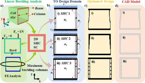
The design process starts with conducting a linear buckling analysis on 2D SHC SC to investigate in-plane buckling. This analysis aims to examine the morphologies of buckling modes and identify the members that are most susceptible to buckling under compressive loading and demonstrate maximum deformation. In this study, we utilised ABAQUS software to construct the FE model of the SC, employing plane strain elements for all members, as depicted in Figure 2(a). The chosen cell size is 60 mm, with beam thickness of 4 mm and columns with a thickness of 2.5 mm to achieve a relative density of approximately 20%. The structure is subsequently modelled using 6-node modified quadratic plane strain triangle elements (CPE6M) with plane strain thickness 60 mm and an element length of 2 mm. The material properties were taken as Young's modulus of 1 GPa and a Poisson's ratio of 0.39. The BCs on FE model are not periodic, as we consider the SC as an independent structure, and instead applied as a compressive load on top surface with fixity on bottom surface schematically shown in Figure 2(b). They are implemented as follows in the software: a reference point is connected to the nodes on the bottom surface, and a rigid body constraint is imposed on this point. Additionally, the top surface is constrained only in horizontal displacement. The loading simulates a compressive test, with the top surface receiving a vertical compressive load of 1N. This load is applied to a master node which is tied to all the other (slave) nodes on the surface. In this initial linear buckling analysis, a 1N compressive load was applied to the master node in the negative y-direction, effectively applying a 1N compressive load to the entire top surface. Figure 2(a) shows these software BCs application which are same as schematic BCs shown in Figure 2(b). In ABAQUS, linear perturbation analysis is used with the ‘buckle’ analysis step to simulate linear buckling analysis. The subspace iteration Eigen solver was selected to extract the first five eigenvalues. Figure 2(a) illustrates the mode shape resembling the compressive buckling pattern. Performing a linear buckling analysis on the base SC assists in finding regions susceptible to buckling. In the SHC SC, since there are no inclined members, the primary members prone to buckling are the two vertical columns. Consequently, the columns of the SC are subsequently modified using TO, as clearly illustrated in Figure 2(b) to achieve an optimal material distribution while preserving the relative density of the SC, as elaborated in the following section.

4.2. Buckling driven 2D TO designs of SHC

We employed the TO process to enhance the buckling strength of the LS, specifically utilising the 2D TO method outlined in Section 4.1. The 2D SHC SC shown in Figure 2(a) is considered as the design domain for TO application consisting of both beams and columns.

The optimisation design domain is defined based on prior knowledge of weak members, which is designated as active regions, while the remaining regions are considered passive regions. The linear buckling analysis (in Figure 2(a)) revealed that the columns are the most vulnerable buckling regions within the SC and are designated as active regions in the TO, where the objective is to maximise the BLFs while adhering to constraints related to compliance (stiffness) and volume fraction. In this context, the beams are considered passive regions, and the void area within the design domain corresponds to the centre of the lattice face. However, within this study, the columns are designated as both active and passive regions in three different ways to explore all possible topologies and determine their respective performance. The cases are as follows:

1. SHC1 – The active regions encompass the entire column area, extending from the top of the base beam to the bottom of the top beam (Figure 2(b-i)).

2. SHC2 – The active column area in SHC1 is complemented by a passive region with a unit or few elements width along its outer edge (Figure 2(b-ii)).

3. SHC3 – The active column area of SHC2 is further provided with a passive region of unit or few elements width along its inner edge, effectively creating a box-like enclosure of the active region within the passive one (Figure 2(b-iii)).

The three initial designs mentioned above are subsequently subjected to TO with BLF maximisation and constraints applied for compliance and volume (area).

Consider the SHC designs illustrated in Figure 2(b), where a SC size, L = 60 mm was selected. The TO square domain is hence discretised by ${\mathrm{\Omega }}_h$ = 60 × 60 elements (nelx x nely). The active region A, solid passive region P₁ and void region P₀ are indicated. The thickness of beams (s₁) are fixed as 4 mm and those of columns (s) of SHC1 and SHC2 as 4 mm and SHC3 as 5 mm (including a 1 mm passive inner wall). We initially achieve an area ratio of 25%, which we aim to reduce to approximately 21% through TO of the columns. However, s is investigated experimentally with values ranging from 4 to 6 mm. This is discussed in greater detail in the next section, which focuses on parameterisation. A distributed load with a magnitude of 1N is applied to the entire top surface. We set E₀ = 1 GPa and E_min = 10⁻⁶ GPa, ν = 0.3 and r_min is chosen as 3 for this mesh size. As explained previously, we first obtain a minimum volume design starting the TO process with full solid elements (density = 1) in the active regions for a fixed C_max/C₀, with minimum area fraction as 16.6%, 18.6% and 20.8% for SHC1, SHC2 and SHC3 respectively. The resulting optimised topology is saved as ‘xInitial’ in a mat file named ig.mat.

Next, BLF maximisation is carried out to enhance the design's resistance against buckling. This is accomplished by utilising the initial topology, adjusting the parameter β = 6 and its continuation parameters {400,24,25,2} [27]. Additionally, an area (for 2D, all volume notations in V refers to area) constraint is imposed, with V_max set at 21%, surpassing the maximum area of 20.8% attained in the minimum area design. The objective is to achieve buckling-resistant columns while maintaining a consistent area fraction across all designs. The resulting optimised designs are also shown in Figure 2(c)-(i) SHC1, (ii) SHC2, and (iii) SHC3.

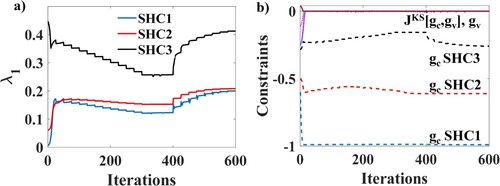
The plots of the evolution of the fundamental BLF ${\lambda }_1$, the constraints $\mathrm{gv},\mathrm{gc}$ and the aggregated constraint $J_1^{\mathrm{KS}}([\mathrm{gv},\mathrm{gc}])$ during the buckling reinforced TO are shown in Figure 3 for the three designs to study their buckling resistance. The BLF exhibits an improvement relative to their initial minimum volume design for both SHC1 and SHC2 during the optimisation process. Although the BLF initially decreases for SHC3, it ultimately reaches the same value as the initial design by the end of the optimisation process. Moreover, it notably exceeds the values achieved for both SHC1 and SHC2, indicating a greater buckling strength for the SHC3 design. The rise after 400 iterations maybe due to continuation parameters introduced after 400 iterations. The constraint $\mathrm{gv}$ coincides with $J_1^{\mathrm{KS}}([\mathrm{gv},\mathrm{gc}])$ and remains at zero for all the designs. On the other hand, the compliance constraint $\mathrm{gc}$, represented by dotted lines, also demonstrates that SHC3 with near zero $\mathrm{gc}$ follows best compliance constraint compared to the other two designs.

Figure 3. Evolution of (a) first BLF and (b) constraints for buckling maximisation TO of SHC1, SHC2 and SHC3 of 60 × 60 mesh.

The total computational cost for running the buckling optimisation (600 iterations) was very low due to the small mesh size, taking only 278 s for all the designs on a workstation equipped with an Intel(R) Xeon(R) E5-2650 v2 @ 2.60 GHz CPU, 64 GB RAM, and MATLAB 2022a running in serial mode on Windows 10. This efficiency is attributed to the speedups implemented in the MATLAB code by developers, such as fast assembly implementation and the use of volume-preserving filters. These enhancements ensure that the eigenproblem utilises most of the computational time, further improved with a highly efficient eigensolver [27]. In comparison to the example in [27] with a compressed column of 480 × 240, which took 12,900 s for the entire buckling computation, our computational time was significantly reduced due to the smaller domain sise with a central void space. Therefore, porous lattice designs will consistently yield much faster computational times than solid domains, regardless of the mesh size used.

5. 2D FE analysis

The 2D CAD models of SHC1, SHC2, and SHC3, smoothened out from the above obtained TO designs (Figure 2(d)) are now subjected to a 2D plane strain analysis in ABAQUS following the same elements, material properties and BCs detailed in Section 4.1 for the linear buckling analysis. To assess the variation in buckling strength compared to the reference design, an SHC model was also created with a modified column width of 2.65 mm to ensure the same area fraction of 21%. The first mode shapes for all designs are illustrated in Figure 4(a). Utilising this mode information, a post-buckling analysis is conducted in ABAQUS, employing static Riks analysis to account for nonlinear material yield behaviour. Arbitrary plastic stress–strain data was also provided to introduce a post-buckling material yield behaviour, with a yield stress of 35 MPa and an isotropic linear hardening modulus of 800 MPa. The ABAQUS input file utilises the *IMPERFECTION keyword under the Step command to introduce slight structural perturbations equivalent to the first three modes, scaled by factors of 0.05, 0.02, and 0.001, respectively. The applied load is now modified to match the first eigenvalue, calculated from the linear buckling analysis. The load-displacement plots from this analysis are shown in Figure 4(b), with the buckling strength represented by the maximum point on the load vs. deflection curve.

Figure 4. Numerical analysis with preliminary designs: (a) Linear Buckling modes, (b) Post buckling analysis.

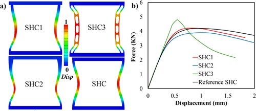
Amongst the designs, SHC3 exhibited the highest buckling strength, surpassing the reference SHC by 15%. The SHC2 sections displayed an identical strength, while SHC1 exhibited a lower strength, similar to the base reference model. These findings indicate that further exploration of TO parameters may yield additional designs with enhanced buckling performance, similar to SHC3. The parameters of mesh size and TO parameter r_min, require experimentation in this study. In the preliminary analysis, we established fixed values for the mesh size and filter radius and obtained buckling-driven TO designs for three cases of 2D SHC, as shown in Figure 2(c). In the next section, we detail their parameterisation in order to generate a family of designs.

6. Parametric study

6.1. TO parameter – maximum compliance ratio

The maximum compliance ratio C_max/C₀ for different designs was varied from 1 to 2, in order to determine the optimal value for minimising volume while maintaining structural integrity. This ratio differed for each case as 1.4–2.0 for SHC1, 1.3–2.0 for SHC2 and 1.2–1.4 for SHC3. However, it's important to note that increasing the ratio beyond the above range resulted in a rapid convergence of the TO process in fewer than 10 iterations, without any improvement in the base design. For example, SHC3 could only accommodate values up to 1.4. When the maximum allowed compliance limits are set too low, they impose constraints that limit design freedom, ultimately resulting in lower BLF [27]. Therefore, in order to maximise the design freedom while maintaining a uniform upper compliance limit for all designs, we selected the maximum possible value observed in the SHC3 design, which was 1.4, as the upper compliance limit for all designs.

6.2. TO parameter – FE mesh

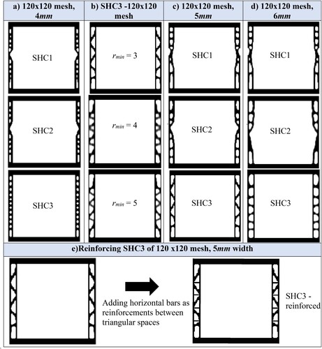
In the initial phase of the study, a FE mesh of 60 × 60 was adopted. However, as we progressed, we found it necessary to refine the mesh to 120 × 120, while keeping all other parameters constant. This means that the cell size remains the same 60 mm, but instead of discretising Lx with 60 elements, we divide Lx into 120 elements and same applies for Ly too. The computational time for the buckling analysis has now increased to 974 s for this finer mesh size, though it still does not pose a computational burden. Figure 5(a) illustrates the three distinct designs we obtained for a column thickness of 4 mm. These designs showcase denser columns while maintaining a constant relative density across all three cases. The effect of refining the mesh size also shows improvement in BLF (comparing Figure 3(a) to Figure S1), the BLF increases. Notably, the topologies of SHC1 and SHC2 closely resemble each other in design, indicating that the incorporation of an external passive wall was unnecessary, as it naturally evolved during the optimisation process. In practical terms, during fabrication, both the SHC1 and SHC2 designs can be treated as a single design for 4 mm width.

Figure 5. Parameterisation studies.

6.3. TO parameter – filter radius

Next, we conducted tests for the filter radius, r_min, using both the 60 × 60 and 120 × 120 mesh sizes to determine the appropriate value (see Supplementary information for 60 × 60 mesh results). We observed that a lower r_min resulted in an asymmetrical topology, while a higher r_min yielded a denser topology with a higher area fraction (as depicted in Figure 5(b) for 120 × 120 mesh and Figure S4 for 60 × 60 mesh). As a result, we chose r_min = 3 for both mesh sizes because this radius value consistently produced a unique 0–1 topology. In subsequent discussions, when the column thickness is modified, further experimentation with r_min is necessary to determine its suitability for the chosen thickness.

6.4. Geometry parameter – thickness of column

We conducted experiments with an increased mesh size to assess the potential for enhancing buckling resistance by accommodating greater compliance limits, achievable by using thicker columns and a refined mesh. Specifically, we examined column thicknesses of 5 mm, 6 mm, in addition to the previously analysed 4 mm. Figure 5(c,d) displays the resulting designs of SHC1, SHC2, and SHC3 for the 5 and 6 mm column configurations, respectively. As with the 60 × 60 mesh designs, we determined the volume fraction based on the maximum volume fraction achieved among the corresponding minimum volume TO designs for each configuration. The SHC3 design with a 6 mm thickness achieved a maximum relative density of 21.2%, leading us to set the upper optimisation volume limit at 22% for all 120 × 120 mesh designs, irrespective of thickness. As a result, the reference dimension for the column width in the equivalent SHC, used for comparison, was 3 mm to achieve a relative density of 22%. As outlined in section 6.3, we experimented with r_min= 3 for the new thicknesses, determining that r_min= 3 was suitable for 5 mm, while r_min= 4 was optimal for the 6 mm thickness. The C_max/C₀ ratio was maintained at 1.5. In addition to the designs generated through TO, we introduced a modified design for the 5 mm-width SHC3, incorporating horizontal stiffeners within the triangular gaps of the columns, denoted as SHC3-Reinforced, Figure 5(f).

The BLF plots (see Figure S1 in Supplementary information) from the TO analyses of the three thicknesses showed an increase in BLF with column width and they were also higher than that of the 60 × 60 mesh investigated in Figure 3. This indicates that increasing column width may help to enhance the buckling resistance. We now fabricate the designs to validate the conclusions made from the linear buckling analysis-based TO process.

7. 3D Analysis

7.1. Fabrication and experimental testing

The investigation focusing on varying key parameters in the previous section provided insight into the selection of their values for each TO design. With the knowledge gained, selected designs of SHC1, SHC2, and SHC3 for 120 x120 mesh with varying wall widths were manufactured to experimentally determine their buckling resistance, all designed at a 22% volume fraction and those of 60 × 60 mesh manufactured for 21% volume fraction.

AM based on the Material Extrusion process, as defined by ASTM 52900 [37], was adopted to manufacture all specimens. The Material Extrusion process, also known as the Fusion Deposition Modelling (FDM) process, works by extruding a molten filament of polymer material to selectively trace out the layers of the part, fabricating the 3D physical models. In this study, we employed the Creality Ender-3 V2 3D printer and used Nylon White filaments provided by Markforged, USA. The material is an unfilled thermoplastic with a density of approximately 1.1 g/cm³, low modulus, and high failure strain, allowing for a more ductile response. The printer is capable of achieving a printer accuracy of 100 microns. The process parameters of FDM include build orientation, layer thickness, air gap, print speed, and extrusion temperature [38], all carefully selected as discussed. Other process parameters such as raster angle and width, contour width and number, are automatically evaluated by the printer based on geometry.

Firstly, the 2D TO designs are converted to 3D CAD models using Fusion 360 software. Post-processing of the designs includes smoothing edges (Figure 6(a)) to remove step-like edges typically generated by TO. The CAD files were then exported as stereo lithography (STL) file format and sliced using Super Slicer 3D printing software (version 2.4.58.5) before being transferred to the Ender-3 printer. In the printer, the polymer filament is fed into a heated extruder with a temperature of 270°C by the motor driving force from a coil reel, and transferred into molten paste to be extruded from the nozzle tip with a diameter of 0.4 mm. The print speed was set at 40 mm/s, and the part cooling fan was deactivated. The extruded material is squeezed onto the base plate, which is set at a temperature of 70°C, line by line based on the pre-designed tool-paths to form a surface, and finally, the 3D part. After one layer has been completed, the extruder is lifted by a distance of the layer thickness set as 0.2 mm to deposit another layer. Due to the fact that the TO designs were 2D designs simply extruded in the Z-direction to make the 3D models, it was convenient to orient the build direction along the extruded Z-direction (Figure 6(b)), thereby alleviating the need for any support material and eliminating overhangs in prints. Subsequently, the samples were dried in a convection oven at 80°C for 5 h and then stored in a desiccator before testing.

Figure 6. DFAM considerations (a) Smoothening of sharp step edges of TO design (b) Build orientation to prevent need for support structures (c) Minimum feature size and printing defects (d) Removing designs with very thin wall thickness (e) Weights of 3D printed designs.

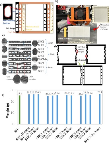
Finally, the specimens were weighed using an OHAUS Scout Pro scale, and their external dimensions were measured using a digital Vernier caliper with an accuracy of 0.01 mm. The minimum feature sizes were checked using an optical microscope, and they are listed in Figure 6(c) for all specimens. Some of the manufacturing defects obtained included over-extrusion, resulting from extruding while moving the print head in a tight area, and under-extrusion, caused by the relatively high printing speed. Additionally, rounding of sharp corners was observed, as shown in Figure 6(c).

Taking into account the DFAM considerations, especially the AM constraints, further parametric studies of TO designs were conducted, in addition to those discussed in the previous section. For instance, the thin wall sections of the SHC1, SHC2, and SHC3 structures were required to adhere to the printability limit of 0.4 mm, which is the minimum feature size possible due to the nozzle diameter. However, the minimum wall thickness of passive regions during TO was initially set at 0.5 mm, resulting in sections that were too thin after TO, very close to the minimum printability limit (Figure 6(d)). Additionally, when subjected to FE analysis, these thin sections exhibited undesirable local buckling. Consequently, the thickness of the passive region was increased to 1 mm, which, after accommodating for smoothening by rounding curves in some void parts, was further reduced to approximately 0.65 mm in the CAD design and measured as 0.7 mm in the printed part. It was once again ensured that this new thickness did not cause any local buckling or violate minimum feature limit constraints. Here, a unit cell size of 60 mm × 60 mm × 30 mm was chosen to ensure that all samples could be printed within the minimum feature size of 0.4 mm. In the future scope of continuing work, when this study is extended to multi-cell lattice structures, the unit cell will be chosen in such a way that reducing cell size at the part level design does not compromise printability.

Tensile tests were essential for assessing the mechanical properties of the parent material required in the FE simulations. Accordingly, adhering to ASTM D638 standards, we manufactured six dog-bone specimens flat on the build plate to obtain the Young's modulus and Poisson's ratio. The specimens were fabricated using the same print parameters as were used to fabricate the SHC structures to ensure the applicability of the obtained results. Finally, the measured weights of the printed specimens (Figure 6(e)) were kept in check to ensure they did not deviate much from each other and the actual CAD weight of 26.14 g.

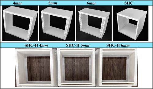
The 3D CAD designs of optimised designs and the SHC3 Reinforced design along with their 3D printed samples for 120 × 120 mesh are shown in Figures S3 and S4, respectively of supplementary information. Few representative 3D printed samples among them are depicted here in Figure 7 along with their reference SHC with wall width 3 mm for finer mesh design. The 3D CAD and printed models of optimised designs for 60 × 60 mesh are also shown in Figure S6. The reference SHC shown in Figure 7 is a solid wall section whereas the TO designs of different wall thickness is with hollow thin walls. Hence for a fair comparison, we also manufactured hollow thin wall structures of 4, 5, 6 mm wall thickness, named SHC-H along with thickness (Figure 7), to compare with the hollow TO designs of similar wall thickness.

Figure 7. Few representative 3D printed specimens extruded from the 2D designs of 120 × 120 mesh SHC3 designs for different wall widths and Reference SHC with solid wall and hollow walls.

7.2. Numerical validation

From the experimentally tested designs, the best-performing configuration among the three design cases for all wall widths of 4, 5, and 6 mm, is modelled using ABAQUS for numerical validation and compared with reference SHC SC. A 3D analysis is conducted using C3D10M elements (10-node modified quadratic tetrahedron) for the side walls and C3D20R elements (20-node quadratic brick element, reduced integration) for the top and bottom walls. The material properties, loading, and BCs are the same as those outlined in Section 4.1. The analysis included both a linear buckling analysis and a post-buckling analysis.

8. Results and discussions

8.1. Experimental results

The SHC SC designs, previously discussed with a volume fraction of 21% for 60 × 60 mesh and 22% for 120 × 120 mesh, were manufactured and subjected to uniaxial compression tests to assess their buckling strength. These were compared with solid wall cross-sections with equivalent volume fractions. Figure 8(a–c) displays the force vs. displacement diagrams for designs in various wall widths within the 120 × 120 mesh. The experimental results of the 60 × 60 mesh are shown in Figure S7 of supplementary information. In all samples, the force increased till it reached a maximum load, known as the critical buckling load, beyond which structure loses its load carrying capacity. This critical buckling load was highest for SHC3 among all wall thicknesses, hence indicated SHC3 design is the most buckling-resistant topology among all designs. Each specimen exhibited varying post-buckling responses, depending upon the column's geometry, hence a detailed study of the buckling patterns follows.

Figure 8. Experimental results. Force vs displacement curves for 120 × 120 mesh topologies of (a) 4 mm, (b) 5 mm, (c) 6 mm, (d) Comparison of best performing design SHC3 for various widths and reinforcement.

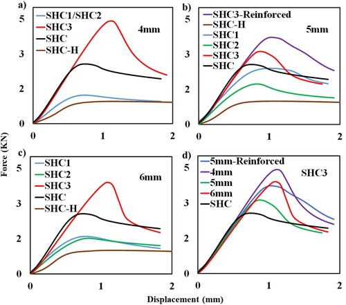
Notably, the rate of load reduction following the critical buckling load was most pronounced in SHC3, followed by samples SHC, SHC2, and SHC1, respectively. Furthermore, within the refined mesh, SHC2 was the initial design to fracture upon buckling, with the crack originated at the location of the highest stress concentration around the neck of its geometry. The poor performance of SHC1 and SHC2 can also be attributed to these neck-like regions, which were the first to undergo bending and resulted in column buckling. Conversely, SHC3 had a uniform thickness throughout, and buckling occurred only in regions with hollow sections within the thickness. Therefore, the reinforced variant of SHC3 demonstrated significantly enhanced buckling resistance compared to its unreinforced counterpart, as these hollow sections were further reinforced. All the best-performing SHC3 designs exhibited a significantly higher buckling resistance, with an improvement ranging from 30% to 70% when compared to the reference solid wall design as illustrated in Figure 8(d). Surprisingly, the most robust performance came from the 4 mm width design, contradicting the assumption that wider columns would inherently exhibit a greater buckling resistance. This discrepancy may be attributed to the fact that unlike the linear buckling analysis which developed the topologies, the nonlinear material properties along with the geometry of the new designs come into play during compression. The post-buckling analysis may depend on factors like the dense lattice topology of the 4 mm width wall, which effectively acted as reinforcement against buckling whereas the 6 mm walls had bigger void regions and thin walls in their topology, causes them to buckle sooner. The manually added reinforcement to the 5 mm design resulted in a slight improvement in buckling resistance compared to the 5 mm width design, yet it still did not surpass the performance of the 4 mm design. These results were subsequently validated through a complete post-buckling analysis in numerical simulations. Figure 8 illustrates the critical loads for the reference hollow structures (SHC-H) with column widths of 4, 5, and 6 mm, reveals a strength of approximately 1 KN, the lowest among all other designs. Therefore, a more suitable reference would be SHC with solid walls.

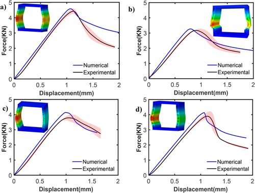
8.2. Comparison of numerical and experimental results

Figure 9 displays load-displacement plots for all designs obtained from both the post-buckling numerical analysis (bold lines) and the experimental study (dotted lines), accompanied by the first mode shapes obtained through linear buckling analysis. As anticipated, the mode shapes are susceptible to buckling in the narrow regions within the topology. The numerical study successfully validates the experimental work. It is worth noting that specimens’ conditions can influence various aspects of buckling performance, including build quality and surface roughness of the structure. As a result, minor discrepancies between experimental and numerical results are observed, but they fall within an acceptable margin of a 10% deviation.

Figure 9. Comparison of experimental and numerical results for best performing SHC3 for (a) 4 mm, (b) 5 mm (c) 5 mm Reinforced and (d) 6 mm along with the first mode shapes from linear buckling analysis.

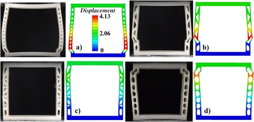
Furthermore, we compare the experimental evolution with numerical compression displacements, as illustrated in Figure 10, with a post-buckling strain of 2%. Buckling occurred for all structures within a strain range of 1.5% to 1.8%. The deformation patterns closely matched between experimental and numerical results, indicated that the numerical modelling effectively represents the mechanical behaviour during compression.

Figure 10. Comparison of experimental and numerical results for best performing SHC3 for (a) 4 mm, (b) 5 mm (c) 5 mm Reinforced and (d) 6 mm for postbuckling strain of 2%.

Despite the fact that 4 mm width walls exhibits the highest critical buckling load, it demonstrates greater post-buckling displacements compared to the reinforced design and the 6 mm design. This phenomenon may be attributed to the fact that the 4 mm width design, after reaching the critical load, experiences a more rapid buckling, which result in a more significant drop in strength compared to the other designs.

In summary, the primary objective of this study is to enhance the load-carrying capacity of members susceptible to buckling within the structure. This is achieved by transforming their simple solid topologies into configurations resistant to buckling through optimisation techniques. The presented approach focuses on the utilisation of a single-cell structure inspired by the unit cell shape of a square hexagon periodic lattice structure. The single cell is not treated as a part of the lattice but as an independent structure for the examination of buckling patterns in members. TO is employed to make these members buckling-resistant. The study specifically addresses the global buckling mode of a single cell and the optimisation of its buckling region through TO. No periodic boundary conditions are applied, and multiple-cell lattice structures are not considered in this work. Therefore, the study's results cannot be directly extrapolated to multiple-cell lattices since periodicity is not taken into account. To correctly optimise the topology for a periodic lattice, periodic boundary conditions must be applied during the TO of a single cell. This process results in a different material distribution, leading to distinct column topologies compared to those obtained in this study.

The successful demonstration in our study contributes to the development of lightweight, buckling-resistant single-cell lattice structures. It is crucial to note that this study operates at a single-cell level, establishing a pathway for designing unit cells and periodic lattices in future research.

A potential future direction for this research involves expanding beyond the single-cell study to include part-level design. However, this may necessitate extensive research efforts. The authors are working on extending the current study to explore the effects of periodicity on the single cell, making it a unit cell, and investigating the overall buckling behaviour of lattice structures with more than two cells. This include study of cell interactions, local buckling of unit cells, and the impact of cell size and number of cell arrays. Future research directions also include testing three-dimensional topology optimisation and enhancing the buckling strength of inclined members in strut-based lattices and shell-based triply periodic minimal surface within the three-dimensional topology space.

9. Applications and scalability of method

While this study focuses on a single-cell structure, extending the applicability of the results to multi-cell or whole-structure scenarios requires further research. Future directions may involve broadening the scope beyond single-cell analysis to include part-level design of larger lattices, although this may entail significant research efforts. Additionally, manufacturability limitations of large 3D structures must be considered. The authors are currently extending the study to investigate the effects of periodicity on single cells, transitioning them into unit cells, and exploring the overall buckling behaviour of lattice structures with more than two cells. This entails studying cell interactions, local buckling of unit cells, and assessing the impact of cell size and the number of cell arrays.

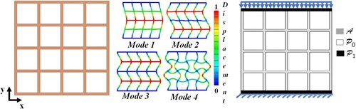
An example of a larger structure with a multiple-cell (4 × 4) lattice, as depicted in Figure 11, can illustrate the applicability of the proposed methodology. Initially, the multi-cell structure undergoes linear buckling analysis to identify its modes. By examining the first few modes, various active–passive domain combinations for optimisation are determined. Figure 11(c) shows one possible combination, where the top and bottom beams are passive, while inner members have an outer passive boundary of 1 mm, inspired by the best-performing design (SHC3) from the single-cell study in this paper. However, other combinations can also be explored by assessing the extent of buckling in different members across different mode shapes. By selectively assigning members with lower buckling (closer to supports) as active domains and those with higher buckling (centre) as passive–active combinations, the optimal buckling-resistant design can be achieved.

Figure 11. Potential future extensions: Scaling the present methodology to a 4 × 4 cell lattice structure. (a) CAD design of the lattice to be optimised (b) first four linear buckling modes and (c) active–passive-void design domains for TO.

Future research directions also include testing 3D topology optimisation (3D TO) and enhancing the buckling strength of inclined members in strut-based lattices and shell-based triply periodic minimal surfaces within the 3D topology space. This involves changing the finite element (FE) discretisation of TO to 3D elements and recalculating the buckling load factors (BLFs). Additionally, the use of different grid types other than the square grid lattice discussed above can be experimented with in this future scope of work. Various buckling-based optimisation studies on lattice structures of different grid types, such as Kagome core [39], Kirigami patterns [40], and hierarchical patterns [22], exist in the literature and can be compared when extending the current method to 3D TO.

Therefore, scaling the proposed optimisation approach from 2D single-cell thin-walled structures to multiple-cell lattice structure, and further extending it to larger and more complex 3D structures with struts or shell-based surface lattices using 3D topology optimisation (3D TO), will represent the most significant contribution to the research of buckling-resistant lattice structures for engineering applications.

Having discussed the scalability of the methodology presented in this paper, it is pertinent to mention that computational costs can significantly increase when scaling the single-cell structures studied here to larger lattices. This aspect has already been investigated by the developers of the MATLAB code in [41,42]. Additionally, one could explore parallel computing on multicore CPUs for solving the eigenproblem [43]. Although scaling the problem from 2D to 3D topology optimisation (TO) will also escalate computational costs, the work of Ferrari et al. [27] discusses that their code is efficiently prepared to handle 3D TO computations due to the efficient utilisation of cheap vectorised matrix products and sparse storage and computations within the code.

10. Conclusions

In this study, we introduced an innovative methodology for designing buckling-resistant LSs using TO. This novel TO-based approach showcases the potential of harnessing the buckling behaviour of cellular structures to create lightweight and buckling-resistant lattice designs. Specifically, we applied this methodology to SHC LSs. We harness the inherent buckling modes within the thin wall of SHC to inform the design of modified stiffened LSs, resulting in an enhanced buckling resistance.

We generated a series of designs through a parametric study, considering optimisation parameters such as the buckling member's thickness and the active domain for optimisation. While designing and fabricating these structure, considerations of DFAM such as AM constraints of minimal feature size, the need for supports, and overhangs were also taken into account. Contrary to the assumption that wider columns inherently offer greater buckling resistance, the 4 mm width design unexpectedly exhibited the strongest performance. This unexpected result can be attributed to the dense lattice topology of the 4 mm width column, which effectively reinforced it against buckling. In contrast, the 6 mm columns featured large void regions and thinner walls in their topology, leading to earlier buckling. Experimental analysis of additively optimised LSs demonstrated an impressive 70% enhancement in buckling strength, all while maintaining stiffness and weight. Numerical simulations further validated these results, showing a negligible deviation of less than 10%. Our findings highlight the potential of this methodology to create innovative LSs with significantly improved buckling resistance while maintaining their stiffness.

Disclosure statement

No potential conflict of interest was reported by the author(s).

Data availability statement

The data that support the findings of this study are available from the corresponding author upon reasonable request.

Additional information

Funding

This publication is based on work supported by the Khalifa University of Science and Technology [award No. CIRA-2021-109 / 8474000423].

References

- Ashby MF, Medalist RFM. The mechanical properties of cellular solids. Metall Trans A. Sep. 1983;14(9):1755–1769. doi:10.1007/BF02645546
- Nazir A, Abate KM, Kumar A, et al. A state-of-the-art review on types, design, optimization, and additive manufacturing of cellular structures. Int J Adv Manuf Technol. Oct. 2019;104(9):3489–3510. doi:10.1007/s00170-019-04085-3
- Nazir A, Jeng J-Y. Buckling behavior of additively manufactured cellular columns: experimental and simulation validation. Mater Des. Jan. 2020;186:108349. doi:10.1016/j.matdes.2019.108349
- Eremeyev VA, Turco E. Enriched buckling for beam-lattice metamaterials. Mech Res Commun. Jan. 2020;103:103458. doi:10.1016/j.mechrescom.2019.103458
- He Y, Zhou Y, Liu Z, et al. Buckling and pattern transformation of modified periodic lattice structures. Extreme Mech Lett. Jul. 2018;22:112–121. doi:10.1016/j.eml.2018.05.011
- Manickarajah D, Xie YM, Steven GP. Optimisation of columns and frames against buckling. Comput Struct. Mar. 2000;75(1):45–54. doi:10.1016/S0045-7949(99)00082-6
- Bertoldi K. Harnessing instabilities to design tunable architected cellular materials. Annu Rev Mater Res. 2017;47(1):51–61. doi:10.1146/annurev-matsci-070616-123908
- Viswanath A, Khalil M, Al Maskari F, et al. Harnessing buckling response to design lattice structures with improved buckling strength. Mater Des. Aug. 2023;232:112113. doi:10.1016/j.matdes.2023.112113
- Bendsøe MP, Triantafyllidis N. Scale effects in the optimal design of a microstructured medium against buckling. Int J Solids Struct. Jan. 1990;26(7):725–741. doi:10.1016/0020-7683(90)90003-E
- Neves MM, Rodrigues H, Guedes JM. Generalized topology design of structures with a buckling load criterion. Struct Optim. Oct. 1995;10(2):71–78. doi:10.1007/BF01743533
- Mitjana F, Cafieri S, Bugarin F, et al. Topological gradient in structural optimization under stress and buckling constraints. Appl Math Comput. Nov. 2021;409:126032. doi:10.1016/j.amc.2021.126032
- Gao X, Li L, Ma H. An adaptive continuation method for topology optimization of continuum structures considering buckling constraints. Int J Appl Mechanics. Oct. 2017;9(7):1750092. doi:10.1142/S1758825117500922
- Gao X, Ma H. Topology optimization of continuum structures under buckling constraints. Comput Struct. Sep. 2015;157:142–152. doi:10.1016/j.compstruc.2015.05.020
- Sekimoto T, Noguchi H. Homologous topology optimization in large displacement and buckling problems. JSME Int J Solid Mech Mater Eng. 2001;44(4):616–622. doi:10.1299/jsmea.44.616
- Bruns TE, Sigmund O. Toward the topology design of mechanisms that exhibit snap-through behavior. Comput Methods Appl Mech Eng. Sep. 2004;193(36):3973–4000. doi:10.1016/j.cma.2004.02.017
- Kemmler R, Lipka A, Ramm E. Large deformations and stability in topology optimization. Struct Multidisc Optim. Dec. 2005;30(6):459–476. doi:10.1007/s00158-005-0534-0
- Bian X, Fang Z. Large-scale buckling-constrained topology optimization based on assembly-free finite element analysis. Adv Mech Eng. Sep. 2017;9(9):1687814017715422. doi:10.1177/1687814017715422
- Xu T, Lin X, Xie YM. Bi-directional evolutionary structural optimization with buckling constraints. Struct Multidisc Optim. Mar. 2023;66(4):67. doi:10.1007/s00158-023-03517-9
- Neves MM, Sigmund O, Bendsøe MP. Topology optimization of periodic microstructures with a penalization of highly localized buckling modes. Int J Numer Methods Eng. Jun. 2002;54(6):809–834. doi:10.1002/nme.449
- Thomsen CR, Wang F, Sigmund O. Buckling strength topology optimization of 2D periodic materials based on linearized bifurcation analysis. Comput Methods Appl Mech Eng. Sep. 2018;339:115–136. doi:10.1016/j.cma.2018.04.031
- Wang F, Sigmund O. 3D architected isotropic materials with tunable stiffness and buckling strength. J Mech Phys Solids. Jul. 2021;152:104415. doi:10.1016/j.jmps.2021.104415
- Bluhm GL, Christensen K, Poulios K, et al. Experimental verification of a novel hierarchical lattice material with superior buckling strength. APL Mater. Sep. 2022;10(9):090701. doi:10.1063/5.0101390
- Lindgaard E, Lund E. Nonlinear buckling optimization of composite structures. Comput Methods Appl Mech Eng. Aug. 2010;199(37):2319–2330. doi:10.1016/j.cma.2010.02.005
- Lindgaard E, Lund E, Rasmussen K. Nonlinear buckling optimization of composite structures considering ‘worst’ shape imperfections. Int J Solids Struct. Nov. 2010;47(22):3186–3202. doi:10.1016/j.ijsolstr.2010.07.020
- Luo Q, Tong L. Structural topology optimization for maximum linear buckling loads by using a moving iso-surface threshold method. Struct Multidisc Optim. Jul. 2015;52(1):71–90. doi:10.1007/s00158-015-1286-0
- Wang Y, Sigmund O. Multi-material topology optimization for maximizing structural stability under thermo-mechanical loading. Comput Methods Appl Mech Eng. Mar. 2023;407:115938. doi:10.1016/j.cma.2023.115938
- Ferrari F, Sigmund O, Guest JK. Topology optimization with linearized buckling criteria in 250 lines of Matlab. Struct Multidisc Optim. Jun. 2021;63(6):3045–3066. doi:10.1007/s00158-021-02854-x
- Gibson I, Rosen D, Stucker B, et al. Design for additive manufacturing. In: Gibson I, Rosen D, Stucker B, et al., editors. Additive manufacturing technologies. Cham: Springer International Publishing; 2021. p. 555–607. doi:10.1007/978-3-030-56127-7_19
- Ibhadode O, Zhang Z, Sixt J, et al. Topology optimization for metal additive manufacturing: current trends, challenges, and future outlook. Virtual Phys Prototyp. Dec. 2023;18(1):e2181192. doi:10.1080/17452759.2023.2181192
- Adam GAO, Zimmer D. On design for additive manufacturing: evaluating geometrical limitations. Rapid Prototyp J. Jan. 2015;21(6):662–670. doi:10.1108/RPJ-06-2013-0060
- Mohan SR, Simhambhatla S. Adopting feature resolution and material distribution constraints into topology optimisation of additive manufacturing components. Virtual Phys Prototyp. Jan. 2019;14(1):79–91. doi:10.1080/17452759.2018.1501275
- Bayat M, Zinovieva O, Ferrari F, et al. Holistic computational design within additive manufacturing through topology optimization combined with multiphysics multi-scale materials and process modelling. Prog Mater Sci. Sep. 2023;138:101129. doi:10.1016/j.pmatsci.2023.101129
- Ferrari F, Sigmund O. A new generation 99 line Matlab code for compliance topology optimization and its extension to 3D. Struct Multidiscipl Optim. Oct. 2020;62(4):2211–2228. doi:10.1007/s00158-020-02629-w
- Wang F, Lazarov BS, Sigmund O. On projection methods, convergence and robust formulations in topology optimization. Struct Multidisc Optim. Jun. 2011;43(6):767–784. doi:10.1007/s00158-010-0602-y
- Zienkiewicz OC, Taylor RL, Fox D, editors. The finite element method for solid and structural mechanics. 7th ed. Oxford: Butterworth-Heinemann; 2014. p. i. doi:10.1016/B978-1-85617-634-7.00016-8
- Kreisselmeier G, Steinhauser R. Systematic control design by optimizing a vector performance index. In: Cuenod MA, editor. Computer aided design of control systems. Oxford: Pergamon; 1980. p. 113–117. doi:10.1016/B978-0-08-024488-4.50022-X
- 14:00–17:00. ISO/ASTM 52900:2021. ISO [Internet]. [cited 2024 Feb. 22]. Available from: https://www.iso.org/standard/74514.html
- Huang J, Chen Q, Jiang H, et al. A survey of design methods for material extrusion polymer 3D printing. Virtual Phys Prototyp. Apr. 2020;15(2):148–162. doi:10.1080/17452759.2019.1708027
- Zhang L, Feih S, Daynes S, et al. Buckling optimization of Kagome lattice cores with free-form trusses. Mater Des. May 2018;145:144–155. doi:10.1016/j.matdes.2018.02.026
- Hübner D, Wein F, Stingl M. Two-scale optimization of graded lattice structures respecting buckling on micro- and macroscale. Struct Multidisc Optim. Jun. 2023;66(7):163. doi:10.1007/s00158-023-03619-4
- Ferrari F, Sigmund O. Towards solving large-scale topology optimization problems with buckling constraints at the cost of linear analyses. Comput Methods Appl Mech Eng. May 2020;363:112911. doi:10.1016/j.cma.2020.112911
- Dunning PD, Ovtchinnikov E, Scott J, et al. Level-set topology optimization with many linear buckling constraints using an efficient and robust eigensolver. Int J Numer Methods Eng. 2016;107(12):1029–1053. doi:10.1002/nme.5203
- Li S, Liao X, Lu Y, et al. A parallel structured banded DC algorithm for symmetric eigenvalue problems. CCF Trans HPC. Jun. 2023;5(2):116–128. doi:10.1007/s42514-022-00117-9