Searching optimal process parameters for desired layer geometry in wire-laser directed energy deposition based on machine learning

ABSTRACT

The quantitative prediction of more process parameter variables for fewer layer geometry variables is challenging in wire-laser DED. This study’s novelty is combining machine learning models with a non-dominated sorting genetic algorithm-II (NSGA-II) to predict process parameters for desired layer geometries accurately. Thirty single-layer deposition experiments are conducted to obtain response data of layer geometries to process parameters. Two support vector regression (SVR) models are trained by these data to predict the layer height and width, respectively, and the mean absolute percentage errors (MAPEs) of these models are 4.16% and 1.76%. A reverse system, consisting of both SVR models and the NSGA-II algorithm, is designed to search the optimal process parameters for the desired layer geometries. The maximum MAPE between the actual layer geometry deposited by the predicted process parameters and the desired layer geometry is less than 5.5%, providing solid confirmation of this methodology’s reliability.

KEYWORDS:

• Metal additive manufacturing
• laser directed energy deposition
• process parameters
• layer geometry
• machine learning
• prediction

1. Introduction

As a disruptive manufacturing technique, metallic additive manufacturing (AM) has laid the foundations for the next industrial revolution by forming metal parts with complex structures [1]. Compared to traditional milling or casting manufacturing techniques, metal AM possesses the distinct advantages of a shorter production cycle and a higher material utilisation rate. Generally, the heat sources in metal AM can be supplied by an arc, an electron beam, or a laser [2,3]. Laser AM, which avoids the disadvantages of poor forming accuracy in wire and arc AM and strict vacuum requirements in electron beam AM, is regarded as the most promising metal AM technique [4,5]. Laser powder bed fusion (LPBF) and laser directed-energy deposition (laser-DED) are typical laser AM techniques [6]. LPBF can be used to fabricate complex components with arbitrary geometry. However, it faces the challenges of low production efficiency and high material costs. In contrast, laser-DED is more productive and can provide a larger process parameter window than LPBF.

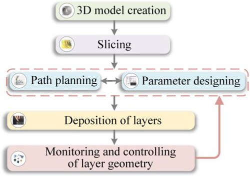
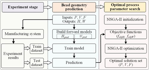
The feedstock in laser-DED can be in the form of wires or powders. Compared with powder-laser DED, wire-laser DED can markedly reduce production costs and escape metal powder’ explosive and flammable risks, which is receiving more attention in manufacturing fields [7]. Many studies have clarified the key factors affecting the deposition layer qualities and improved the intelligence level of metal AM systems [8–10]. An intelligent metal AM system includes four parts, i.e. slicing three-dimensional models, planning deposition paths, designing process parameters, and monitoring and controlling the forming quality of deposited layers (Figure 1). Note that the slicing process of the geometric model determines the deposition layer height, and the path planning process determines the deposition layer width, meaning that the dimension requirements of each deposition path have been given after the path planning is completed. Therefore, one of the central issues of the intelligent metal AM system is how to quickly search the optimal process parameters to fabricate the desired layer width and height.

Figure 1. Schematic diagram of the intelligent metal AM system.

Many models have been established to describe the input-output mapping relationships in metal AM via conventional regression equations [11,12]. In recent years, machine learning (ML) algorithms based on data-driven, such as artificial neural network (ANN), random forest (RF), Naïve Bayes (NB), and support vector regression (SVR) [13–18], have been widely used to solve the classification and regression tasks of multiple objectives by automatically establishing data dependence models. These algorithms possess the merits of excellent self-learning capacity and high adaptability. Table 1 summarises the research on data modelling between process parameters and layer geometries in metal AM. Akbari et al. [15] collected vast amounts of data pairs about process conditions and layer geometry in LPBF from previous reports. They used eight different ML models to estimate the layer geometry from process parameters and material properties, verifying the regression and classification performances of these ML models. Hong et al. [16] used laser power and scanning velocity as inputs of RF and ANN models to predict the layer geometry in LPBF, indicating that the overall R-squared values of these models exceeded 90% on the validation dataset. Zhu et al. [17] established an SVR model to predict the layer height and width by the laser power, travel speed, and powder feed rate in powder-laser DED. A prediction accuracy of 93% was obtained. Liu et al. [18] used the travel speed, laser power, and wire feed rate as both NB models’ inputs to predict the deposited layer height and width in wire-laser DED, indicating that NB models exhibited outstanding regression performances and the R-squared values of both NB models for the layer height and width were 91% and 94%, respectively. The above studies have made some progress in predicting layer geometries based on process parameters in metal AM. However, searching for the optimal process parameters via the desired layer geometry still relies on traditional trial and error methods.

Table 1. Summary of research on data modelling between process parameters and layer geometries in metal AM.

Prediction objects	Ref. & Process	Forward models	Forward inputs	Forward outputs	Reverse systems
Layer geometry	Hong et al. 2023; LPBF.	RF & ANN	Laser power & Scanning velocity.	Layer height & width & Penetration depth.	\
	Zhu et al., 2023; Powder-laser DED.	SVR	Laser power &Travel speed & Powder feed rate.	Layer height & width.	\
	Liu et al., 2022; Wire-laser DED.	NB	Laser power &Travel speed & Wire feed rate.	Layer height & width.	\
Layer geometry & Process parameters	Xiong et al. 2013; Wire arc DED.	ANN	Arc voltage &Travel speed & Wire feed rate.	Layer height & width.	Parameter iterative optimisation based on preset adjusting rules.
	Zhao et al., 2023; LPBF.	MLP	Laser power &Travel speed.	Layer width & Penetration depth.	Step-wise parameter prediction based on the ML model.

The automatic setting of process parameters based on the desired layer geometry, such as the layer height and width, can significantly reduce the time and economic costs caused by traditional trial and error methods. Predicting more process parameter variables from fewer layer geometry variables by data modelling is challenging due to the strong coupling among multiple parameters, resulting in uncertainty in predicted results. A few studies involve the reverse prediction of process parameters based on the layer geometry in metal AM. Xiong et al. [19] designed an iteration optimisation system based on a forward ANN model to predict process parameters for the desired layer geometry in wire and arc AM. However, the iteration optimisation system depends on accurate adjustment rules of the process parameters. Establishing these adjustment rules requires massive experiments and expert experience, limiting the widespread application of this system to predict the process parameters. Zhao et al. [20] used a multi-layer perceptron (MLP) model to step-wise predict process parameters for desired layer geometries in LPBF. First, the desired molten pool width and depth were used as the inputs of the MLP model to predict one process parameter, i.e. the laser power or the scanning speed. Then, the molten pool width and depth, combined with the process parameter predicted in the previous step, were input into the MLP model to predict another process parameter. However, the step-wise prediction method established by Zhao et al. [20] only considers two process parameters and two layer geometries. The capacity to predict more process parameters from given fewer layer geometries was unclear. Besides, these reverse prediction methods can only obtain a unique approximate solution and ignore the diversity of process parameter solutions. Therefore, developing a system that can predict all feasible solutions of more process parameters from given fewer layer geometries without the help of expert experience is highly significant.

To fill the current research gap, a high-efficiency reverse system, consisting of forward prediction models and a non-dominated sorting genetic algorithm-II (NSGA-II), is developed to search all feasible solutions of more process parameter variables for the fewer layer geometry variables without expert experience in wire-laser DED, which is the novelty of this study. Two forward prediction models are trained to respectively predict the deposition layer height and width from process parameters, including travel speed, laser power, and wire feed rate. Then, a closed-loop iteration system, combining two forward prediction models and an NSGA-II algorithm, is designed to predict all feasible optimal process parameter combines for the desired layer geometry. This developed approach can quickly obtain the deposition parameters of the beads with given geometric dimensions in wire laser-DED. This proposed inverse optimisation method that combines ML-based forward prediction models and multi-objective optimisation algorithms holds substantial promise for achieving the collaborative optimisation of forming quality, microstructure, and mechanical properties in laser-DED.

2. Experimental details

2.1. Instrumentation and configuration

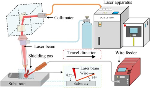
Figure 2 shows a schematic diagram of the wire-laser DED system, including an ABB-IRB4600 robot, an IPG YLS-4000 fibre laser with a wavelength of 1080 nm, and a WF-007A wire feeder. The filler wire was fed in the front feed mode with an angle of 35° to the substrate surface. The angle between the laser beam and the substrate surface was 82°. The laser spot diameter on the substrate surface was 0.6 mm. The distance between the laser spot and the wire tip on the substrate surface was kept at 0 mm to maintain a stable bridging transition of the melted wire. Purity argon with a constant flow rate of 12 L/min was used as the shielding gas. The filler wire was ER70S-6 steel with a diameter of 1.2 mm, and the substrate was Q235 steel with sizes of 300 mm × 100 mm × 6 mm.

Figure 2. Schematic diagram of the wire-laser DED system.

This study aims to establish the relationship between the process parameters and the layer geometries in wire-laser DED. The selected process parameters were the travel speed (V), laser power (P), and wire feed rate (F) since these parameters had significant influences on the layer geometries [21]. The selected layer geometries were layer height (H) and width (W). Table 2 presents the values of the process parameters at different levels. Excessive or insufficient heat input can lead to the molten pool collapse or poor wetting. In contrast, an excessive or insufficient wire feed rate will cause incomplete wire melting or a low deposition rate. The upper and lower limits of the process parameters were determined by performing preliminary deposition trials and inspecting the deposition layers’ appearance. Within these selected process parameter ranges, the sedimentary layer exhibits uniform spreading without obvious geometric defects. Then, six levels were set for each process parameter.

Table 2. The values of process parameters at different levels.

Parameters	Factor levels
	Level 1	Level 2	Level 3	Level 4	Level 5	Level 6
Travel speed V (mm/s)	2.3	2.5	2.7	2.9	3.1	3.3
Laser power P (kW)	2.2	2.4	2.6	2.8	3.0	3.2
Wire feed rate F (cm/min)	120	140	160	180	200	220

As a classic experimental design method for studying multi-factor and multi-level conditions, orthogonal experimental design can select representative points from comprehensive experiments based on orthogonality. These points are evenly distributed in the experimental space and can reflect the fundamental laws of comprehensive experiments [22]. Orthogonal experimental design can significantly reduce experimental costs. Therefore, the orthogonal experiments were performed to efficiently obtain the response relations between the process parameters and the layer geometries. Table 3 displays the designed process parameters and the corresponding layer geometries. Conducting additional testing experiments to check the generalisation performances of the forward models is essential since the actual manufacturing conditions are more complex than the designed training experiments. Eight testing experiments with randomly designed parameter combinations were performed. Table 4 presents the process parameters and measured layer geometries. The length of each deposition bead is 100 mm. Five metallographic specimens were cut from each deposited layer, as presented in Figure 3. The cross-sectional morphologies of the metallographic specimens were captured using a stereomicroscope. The height and width values of these specimens were measured by the Image J software and respectively averaged to reduce accidental errors.

Figure 3. Schematic diagram of the deposited layer geometry.

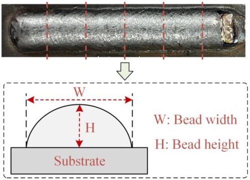
Table 3. Parameter design and results of the training experiments.

No.	P (kW)	V (mm/s)	F (cm/min)	H (mm)	W (mm)
1	2.2	2.3	160	2.77	5.20
2	2.2	2.5	200	3.28	4.72
3	2.2	2.9	140	2.09	5.04
4	2.2	3.1	180	2.64	4.50
5	2.2	3.3	220	3.09	4.17
6	2.4	2.3	140	2.09	6.24
7	2.4	2.5	180	2.79	5.87
8	2.4	2.9	120	1.69	5.84
9	2.4	3.1	160	2.17	5.42
10	2.4	3.3	200	2.53	5.32
11	2.6	2.3	120	1.86	6.75
12	2.6	2.5	160	2.50	6.73
13	2.6	2.7	200	2.88	6.21
14	2.6	3.1	140	1.69	6.28
15	2.6	3.3	180	2.20	5.68
16	2.8	2.5	140	1.77	7.31
17	2.8	2.7	180	2.43	6.71
18	2.8	2.9	220	2.75	6.51
19	2.8	3.1	120	1.47	6.42
20	2.8	3.3	160	1.96	6.59
21	3	2.3	220	3.01	7.24
22	3	2.5	120	1.44	7.95
23	3	2.7	160	1.94	7.56
24	3	2.9	200	2.40	7.17
25	3	3.3	140	1.47	7.07
26	3.2	2.3	200	2.71	7.97
27	3.2	2.7	140	1.73	7.78
28	3.2	2.9	180	2.16	7.59
29	3.2	3.1	220	2.57	6.95
30	3.2	3.3	120	1.25	7.10

Table 4. Parameter design and measured layer geometries of the testing experiments.

No.	P (kW)	V (mm/s)	F (cm/min)	H (mm)	W (mm)
1	2.3	2.5	140	1.98	6.05
2	2.5	2.6	200	2.88	5.85
3	2.6	2.4	220	3.14	6.31
4	2.7	2.8	180	2.55	6.22
5	2.7	3	200	2.72	6.48
6	2.9	2.6	180	2.35	7.15
7	2.9	3.1	160	2.05	6.83
8	3	2.3	200	2.97	7.20

2.2. Forward model for predicting layer geometry

At present, many classic data-driven ML models have been developed to handle classification, regression, and clustering tasks. This section will briefly introduce various ML models and discuss their performances in the next section.

2.2.1. Ridge linear regression ‘ridge’

As a regularised optimisation version of linear regression, ridge linear regression integrates L₂ regularisation method to reduce model overfitting when a small dataset is specified during training [23]. When overfitting appears in a trained model without regulation, the fitting error on the training dataset is quite small since the complex model can learn the features of the training dataset well, but the fitting error on the test dataset is huge. Ridge linear regression imposes a constraint on model parameters to reduce their values, which is beneficial for mitigating the model complexity and overfitting.

2.2.2. Lasso linear regression ‘Lasso’

The Least Absolute Shrinkage and Selection Operator (LASSO) is another regularisation approach utilised to optimise the linear regression model for higher prediction accuracy with less overfitting [24]. Lasso linear regression conducts L₁ regularisation. Due to the L₁ penalty, the model complexity and overfitting can be reduced by nullifying some parameters to achieve the effects of feature selection and dimensionality reduction.

2.2.3. Gaussian process regression ‘GPR’

Gaussian Process Regressor (GPR) is a non-parametric model that uses Gaussian process priors to perform regression analysis on datasets [25]. This model provides a probability distribution of all possible solution values due to its solving process following the Bayesian inference approach and has an excellent prediction performance on small datasets.

2.2.4. Random forest ‘RF’

The Random Forest (RF) model is a ML algorithm based on ensemble learning, and consists of numerous decision trees trained on random sub-samples of the dataset [26]. This model inputs data into decision trees and obtains the final prediction result by voting. For the regression task, the RF model combines the outputs of decision trees and predicts by calculating the average of the outputs. However, when the training dataset is too small, RF is prone to overfitting.

2.2.5. XGBoost

XGBoost is an end-to-end supervised learning model that improves the model’s performance by constructing multiple decision trees [27]. Similar to RF models, XGBoost uses feature column sampling to reduce computational complexity and improve model generalisation. Besides, XGBoost adopts tree regularisation to reduce the probability of overfitting to the dataset.

2.2.6. Support Vector Regression ‘SVR’

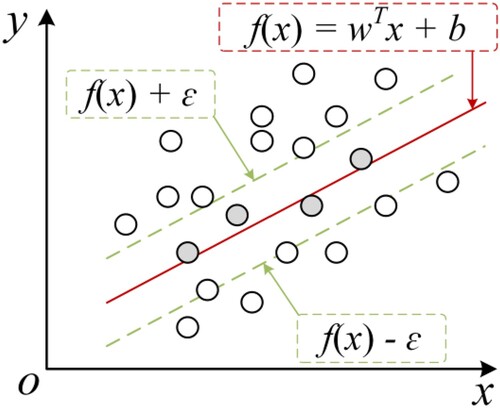
Support Vector Regression (SVR) is a supervised ML algorithm applied for classification and regression tasks [28]. In this study, the SVR model uses the SVM to handle regression tasks of layer geometries in wire-laser DED. It provides a decision boundary at a certain distance from the original hyperplane. Therefore, the sample points nearest to the hyperplane, named the support vector, are within the decision boundary lines [29]. Figure 4 exhibits a schematic diagram of the SVR model where the objective function is represented by a red solid line, and the green dashed line represents the decision boundary with an interval band of width ε.

Figure 4. Schematic diagram of the SVR model displaying the maximising ϵ-interval among the samples furthest from the hyperplane f(x).

The performances of the above-introduced ML models will be tested using the datasets explained previously in the next section. Among them, the optimal model will be used to respectively build a height prediction model (H_pred) and a width prediction model (W_pred) for forward predicting the layer geometry using the process parameters as the inputs. The hyperparameters of the ML models were determined by repeated debugging [30]. Table 5 lists the full parameter sets of various ML models for layer geometry regressions.

Table 5. Parameters of various ML models for layer geometry regressions.

Models	Parameters	Value
Ridge	Alpha	1
Lasso	Alpha	0.02
GPR	Kernel	C(1, (0.01, 0.1)) * RBF(1, (1e-3, 1000))
RF	n_estimators	500
XGBoost	n_estimators colsample_bytree	1000 0.3
SVR	Kernel C	RBF 1000

2.3. Reverse system for searching optimal process parameters

2.3.1. Non-dominated sorting genetic algorithm-II algorithm

This study attempts to use a multi-objective optimisation strategy to address the limitations of the data modelling approach in predicting more process parameters from fewer layer geometries. Traditional multi-objective optimisation algorithms often convert multi-objective problems into a weighted sum of various objectives. Then, the single objective optimisation technique is used to complete the solution. However, the allocation of weighted values for different objectives in these algorithms is highly subjective, and the objectives are constrained by decision variables, resulting in increasing complexity of the weighted objective function’s topological structure [31].

The genetic algorithm developed based on the biological evolution theory has excellent global search capacity, which can avoid falling into local optima issues in traditional multi-objective optimisation algorithms during the optimisation process. Among them, the NSGA algorithm, which introduces non-dominated sorting operators, can give excellent individuals a greater chance of inheritance and better ensure the diversity of the population. In contrast, NSGA-II further integrates fast non-dominated sorting, crowding degree and crowding distance, and elite strategy technologies, improving optimisation efficiency and accuracy [32]. NSGA-II uses a non-dominated sorting algorithm to reduce the computational complexity and merge the parent population with the offspring population, allowing the next generation population to be selected from twice the space. In addition, the elite strategy is introduced to ensure that excellent individuals in the population are not discarded during the evolution process. Therefore, the accuracy of optimisation results is markedly improved. Moreover, the crowding degree comparison operators are used to overcome the limitation of manually specifying shared parameters in the traditional NSGA algorithm and serve as a comparison standard among individuals in the population, allowing individuals in the quasi-Pareto domain to expand to the entire Pareto domain uniformly and ensuring the population diversity (Figure 5). The NSGA-II algorithm mainly includes three key steps, i.e. non-dominance sorting, crowding distance, and elitism operator [33]. NSGA-II possesses the merits of fast running velocity and excellent convergence of solution sets and has been widely used to handle multi-objective optimisation problems in aerospace and machine manufacturing fields [34,35].

Figure 5. Schematic of non-dominated sorting and crowded distance. (a) Non-dominated sorting. (b) Crowded distance.

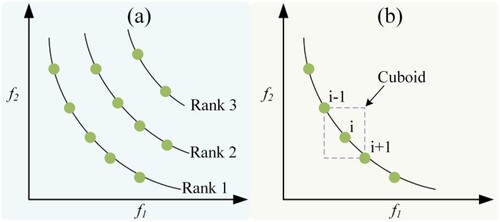
The NSGA-II algorithm considers all Pareto front surfaces instead of only selecting the optimal one, which can ensure the global optimal solutions are obtained. In addition, the solutions in the Pareto optimal solution set, obtained from the NSGA-II optimisation algorithm, are not dominated by any other solutions, meaning that these solutions are not inferior to any other solutions and are regarded as optimal. The hyperparameters of the NSGA-II optimisation algorithm are determined by repeated debugging. In this work, the population size is 100, the maximum number of evolutionary generations is 200, and the mutation probability of mutation operators is 0.2.

2.3.2. Reverse search of process parameters

This study builds a reverse system consisting of the forward H_pred and W_pred models and the NSGA-II algorithm to search the optimal process parameters for the desired layer width and height. Therefore, the approximation problem of the desired layer width and height is converted into the optimisation objective of the NSGA-II algorithm. The objective functions of the layer height and width are defined as (1) $f_{\mathrm{objH}}=|H_d-H_p|$(1) (2) $f_{\mathrm{objW}}=|W_d-W_p|$(2) where f_objH and f_objW are the objective functions of the layer height and width, respectively, H_d and W_d are the desired layer height and width, respectively, and the H_p and W_p are the prediction values of the forward H_pred and W_pred models, respectively. The NSGA-II algorithm is used to search for the optimal solutions to minimise the objective functions f_objH and f_objW simultaneously.

Figure 6 shows the flowchart of the process parameter optimisation for desired layer geometries in wire-laser DED. The fundamental response data pairs are obtained by performing the process design shown in Table 3, and these data are used to train the H_pred and W_pred models. Then, the trained H_pred and W_pred models and the desired layer height and width are used to construct the objective functions f_objH and f_objW. In the search stage for the optimal process parameters, the NSGA-II algorithm generates a number of process parameter combinations called initial population. Note that the process parameters include laser power, travel speed, and wire feed rate, and the reverse prediction of these three parameters is carried out simultaneously. The initial population is input into H_pred and W_pred models to predict the layer geometry and calculate the objective functions f_objH and f_objW. Then, the initial population is performed non-dominated sorting and crowding distance calculation based on the objective functions f_objH and f_objW, and part of the initial population is selected to enter the next generation population based on non-dominated layers and crowding degrees. The remaining part of the initial population is performed cross-mutation and enters the next generation population. The reverse system enters the next iteration when the next generation population reaches the preset size. It outputs the Pareto optimal solution set when the iteration process is completed. The construction and running of the reverse system are carried out on the Python platform using an Intel(R) Core (TM) i7-10870H CPU. The first step of the NSGA-II algorithm is the random initialisation of the parent population, and the search ranges of the process parameters are exhibited in Table 2.

Figure 6. Flowchart of the process parameter optimisation for desired layer geometries.

3. Results

3.1. Forward prediction results

The ML models introduced above are respectively used to construct an H_pred model to predict the layer height and a W_pred model to predict the layer width. Different ML models have varying prediction times at each sample point. Among them, the RF model has the longest prediction time, reaching 2.56 × 10⁻² s, while the prediction times of other models range from 2 × 10⁻⁴–1.2 × 10⁻⁴ s. The shortest prediction time of 1.27 × 10⁻⁴ s belongs to the Ridge model. The performances of these models are checked using the dataset shown in Tables 3 and 4. Table 3 lists the training dataset, and Table 4 exhibits the testing dataset. Accuracy (R²) and mean absolute error (MAE) are used to characterise the model performance quantitatively. The MAE is expressed as. (3) $\mathrm{MAE}={\displaystyle \frac{1}{n}\sum _1^n|G_{A(i)}-G_{P(i)}|}$(3) where $G_{A(i)}$ is the actual layer geometry, $G_{P(i)}$ is the predicted layer geometry, i is the experimental index, and n is the test data number.

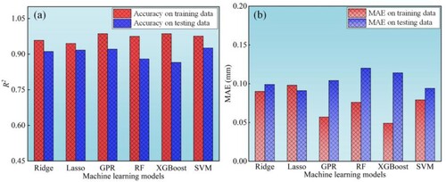
Figure 7 shows various ML models’ accuracy and MAE results for layer height prediction on training and testing datasets. These layer height prediction models present excellent fitting degrees on the training dataset, and the R² values are above 94.5%. The minimum MAE belongs to the XGBoost model, and the R² value is 0.049 mm. However, the accuracy of these layer height prediction models on the testing dataset is lower than those on the training dataset, and the SVM model possesses the highest accuracy, reaching 92.6%. The small amount and noise of datasets are the main reasons for the overfitting of these ML models. ML models are prone to learning features of specific samples or noise, which cannot be generalised to new samples, resulting in slightly lower fitting accuracy in the testing dataset compared to the training dataset. The MAEs of both the SVM and Lasso models are lower than 0.1. Note that the RF and XGBoost models exhibit low generalisation performance on the testing dataset, and both the MAE values of these models are higher than o.11 mm. Overall, the SVM and Lasso models perform better than other ML models in layer height regression.

Figure 7. Accuracy and MAE results of various ML models for layer height prediction on training and testing datasets.

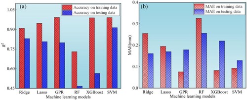
Figure 8 shows various ML models’ accuracy and MAE results for layer width prediction on training and testing datasets. The GPR, XGBoost, and SVR models have excellent accuracy, and the R² values are above 98%. The GPR model has the lowest MAE value of 0.076 mm. The accuracy of the SVM model on the testing dataset is markedly higher than that of other models, and the R² value reaches 92.4%. In addition, compared with other models, RF and XGBoost models are more sensitive to the size of the dataset and are more prone to overfitting on datasets with small volume, resulting in poor fitting accuracy on the test dataset [36]. Compared with other ML models, the SVR model shows apparent advantages in layer width regression. Therefore, the SVR model will be selected to construct the forward prediction model in the reverse system due to its outstanding performance in layer height and width regressions.

Figure 8. Accuracy and MAE results of various ML models for layer width prediction on training and testing datasets.

The above analyses have proven the SVM to be reliable in predicting layer height and width. The section will perform a detailed error analysis of the H_pred and W_pred models constructed by the SVM. The absolute percentage error (APE) and the mean absolute percentage error (MAPE) were used to evaluate the prediction performances of the H_pred and W_pred models. The APE is a percentage value equalling the absolute difference between the actual and predicted values divided by the actual value. The APE is expressed as. (4) $\mathrm{AP}{\mathrm{E}}_{(i)}={\displaystyle \frac{|G_{A(i)}-G_{P(i)}|}{G_{A(i)}}\times 100\text{\%}}$(4) MAPE is defined as the average value of all tests’ APE values. 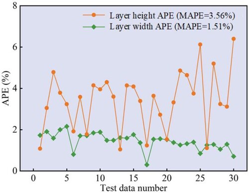The MAPE is expressed as (5) $\mathrm{MAPE}={\displaystyle \frac{1}{n}\sum _1^n\mathrm{AP}{\mathrm{E}}_{(i)}}$(5) Figure 9 illustrates the comparison of the actual and the predicted layer geometries based on the training data. The scatter points are calculated by the H_pred and W_pred models. These scatter points are distributed around the solid lines. The R² values of the H_pred and W_pred models are 99.1% and 97.6%, respectively (Figures 7 and 8). The fitting degree of the W_pred model is better than that of the H_pred model. Figure 10 shows the APE values of the H_pred and W_pred models’ prediction results. The minimum and maximum APE values of the H_pred model are 1.05% and 6.72%, respectively, and those of the W_pred model are 0.45% and 2.34%, respectively. The MAPE values of the layer height and width are less than 3.56%. Both models provide a solid foundation to construct the high-performance reverse system for searching the optimal process parameters for the desired layer geometries.

Figure 9. Predicted results of the H_pred and W_pred models based on the training data. (a) H_pred model. (b) W_pred model.

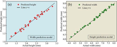
Figure 10. The APE values of the H_pred and W_pred models based on the training data.

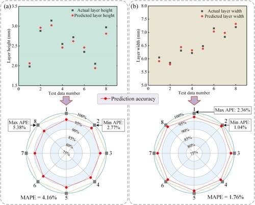
Figure 11 compares the actual and the predicted layer geometries based on the testing data. The predicted points are close to the measured points, indicating a good agreement of the prediction results with the experimental data. A detailed error analysis for the prediction results of the H_pred and W_pred models is performed. The maximum APE values of the H_pred and W_pred models are less than 5.38% and 2.36%, respectively, indicating that the performances of the prediction models can fulfil the engineering application requirements.

Figure 11. Scatter diagrams of actual and predicted layer geometries and prediction accuracy distribution based on the testing data. (a) Layer height. (b) Layer width.

3.2. Reverse prediction results

To realise the automatic setting and optimisation of the process parameters in the intelligent wire-laser DED system, developing a high-efficiency and high-precision approach to predict the process parameters for the desired layer geometries is significant. Four training input-output data pairs are selected from Table 3 to evaluate the prediction accuracy of the reverse system, including No. 10, 15, 20, and 25. The actual layer height and width are input to the reverse system. The reverse system searches the optimal process parameters that can satisfy the minimising of the objective equations f_objH and f_objW by repeated iterations. The reverse system can complete the search process of the optimal process parameters within 3.5 s.

Figure 12 shows the Pareto fronts calculated by the reverse system for different desired layer geometries. Each feasible point represents an optimal solution. The selected point denotes that the optimal solution is selected to validate the performance of the reverse system. The values of the objective equations f_objH and f_objW approach zero, indicating that these objective functions have common solutions, making objective equations’ performances optimal simultaneously. Table 6 lists the process parameters searched by the reverse system. These process parameters range within the variable limits shown in Table 2. Further, the predicted process parameters are input into the H_pred and W_pred models to predict the layer height and width, respectively. The predicted layer geometries are compared with the actual layer geometries to calculate the APE values. As shown in Table 6, there is almost no error between the measured and predicted layer geometries, proving that the developed reverse system for predicting the process parameters based on multi-objective optimisation possesses a superior performance.

Figure 12. Pareto front plots of multiple objective functions under different training experiments selected in Table 3. (a) No. 10. (b) No. 15. (c) No. 20. (d) No. 25.

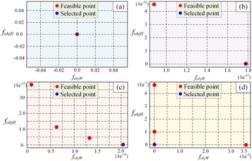
Table 6. Analysis of actual and predicted layer geometries.

No.	Actual geometries		Predicted parameters			Predicted geometries		Error
	H (mm)	W (mm)	P (kW)	V (mm/s)	F (cm/min)	H (mm)	W (mm)	H (%)	W (%)
10	2.53	5.32	2.60	2.83	203	2.53	5.31	0	0.19
15	2.20	5.68	2.89	3.06	157	2.20	5.68	0	0
20	1.96	6.59	2.94	2.56	142	1.96	6.59	0	0
25	1.47	7.07	2.94	2.99	120	1.47	7.06	0	0.14

The results shown in Table 6 demonstrate the reverse system’s feasibility and accuracy. To verify the application capability of the reverse system in the actual manufacturing process, additional eight runs were conducted to predict the optimal process parameters for various desired layer geometries. Table 7 lists the desired layer geometries and corresponding predicted process parameters. These predicted process parameters are within the limits in Table 2. Subsequently, deposition experiments were conducted using the predicted process parameters to obtain the actual layer height and width. Figure 13 shows the cross-sections of single layers deposited by the predicted process parameters. Figure 14 shows the scatter diagrams of the desired and actual layer geometries and corresponding error distribution maps. The actual layer geometries agree with the desired layer geometries, and the maximum APE value is less than 5.5%. The MAPE values of the layer height and width are less than 4.14% and 2.01%, respectively. The errors result from the instability and accidental errors in wire-laser DED and uncertainties in the reverse system. Nevertheless, the accuracy of the reverse system for predicting process parameters is still satisfactory, proving the system’s effectiveness and application potential.

Figure 13. Cross-sections of single layers deposited by the predicted process parameters in Table 7. (a) No. 1. (b) No. 2. (c) No. 3. (d) No. 4. (e) No. 5. (f) No. 6. (g) No. 7. (h) No. 8.

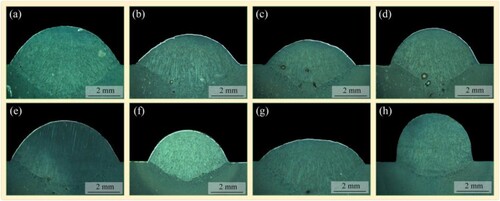
Figure 14. Scatter diagrams of desired and actual layer geometries and corresponding error distribution maps. (a) Layer height. (b) Layer width.

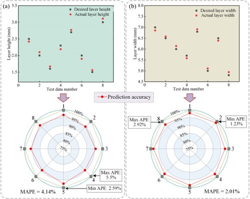
Table 7. Desired layer geometries and predicted process parameters.

No.	Desired layer geometries		Predicted process parameters
	H (mm)	W (mm)	P (kW)	V (mm/s)	F (cm/min)
1	2.5	7.0	2.86	2.52	180
2	2.0	6.5	2.74	3.21	160
3	1.6	6.0	2.58	2.96	121
4	2.3	5.7	2.77	3.20	182
5	2.7	6.8	2.89	2.57	201
6	2.0	5.0	2.20	3.04	139
7	1.5	6.5	2.82	3.15	120
8	3.0	4.8	2.20	2.67	201

3.3. Multi-objective collaborative optimisation framework in laser-DED

This work proposes a reverse optimisation method of process parameters for the desired layer geometries, which successfully achieves rapid optimisation of multiple process parameters. Laser-DED process of large-size components involves sequential multi-layer deposition and intricate thermal processes and includes many optimisation objectives, such as geometric dimension, surface roughness, and tensile strength. Table 8 summarises the controllable parameters and optimisation objectives in laser-DED. The common vision of scholars dedicated to laser-DED is to achieve the collaborative optimisation of forming quality, microstructure, and mechanical properties. Figure 15 shows a flowchart of the collaborative optimisation framework in laser-DED. The key and challenging step is to collect response data sequences of process variables and optimisation objectives. However, obtaining large amounts of data through experiments is expensive and inefficient. Physical model-driven data acquisition methods, such as analytical calculations and numerical simulations, can be used to reduce the data acquisition cost. Besides, selecting process variables and optimisation objectives based on the engineering application requirements can significantly reduce the data volumes.

Figure 15. Flowchart of the collaborative optimisation framework of forming quality, microstructure, and mechanical property in laser-DED.

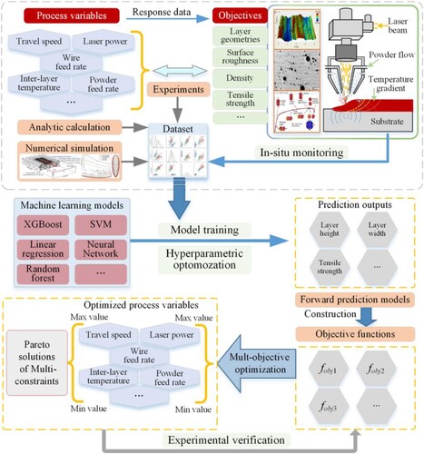
Table 8. Controllable parameters and optimisation objectives in metal laser-DED.

Variables	Objectives
Laser power	Layer geometries
Travel speed	Surface roughness
Powder feed rate	Geometric distortion
Wire feed rate	Grain size
Laser spot size	Phase content
Layer thickness	Density
Layer numbers	Microhardness
Shielding gas flow rate	Tensile strength
Deposition trajectory	Elongation rate
Inter-layer temperature	Corrosion resistance
Materials	Fatigue properties

Subsequently, a forward regression model for each optimisation objective will be established to achieve forward prediction from process parameters to optimisation objectives. Due to the differences in fitting performance of an ML model on different datasets, selecting the appropriate ML models for different optimisation objectives can effectively improve prediction performance. After determining forward prediction models, objective functions are established based on the characteristics of optimisation objectives. The optimisation objectives for extreme value issues, such as surface roughness and tensile strength, are to minimise or maximise the objectives as much as possible. The optimisation objective for specific value issues, such as layer width and height, requires constructing objective functions to transform them into extreme value issues. These optimisation objectives are introduced into multi-objective genetic algorithms as alternative models to achieve collaborative inverse optimisation of forming quality, microstructure, and mechanical properties in metal laser-DED. Furthermore, the in-situ monitoring technique can be integrated with the established optimisation framework to provide feedback on the deviations between the current and target quality states, which is expected to achieve adaptive optimisation of the deposition process in laser-DED.

4. Conclusion

This study aims to develop an approach to automatically search the process parameters for the desired layer geometry in wire-laser DED. Deposition experiments are performed by applying an orthogonal design to obtain the fundamental response data of layer geometries to the process parameters. Various ML algorithms are used to investigate the response relationships between the process parameters and the layer geometries, and the SVR performs better than other ML algorithms on the current dataset. Two SVR models are built to predict the layer height and width by the process parameters, respectively. The results show that the H_pred and W_pred models exhibit excellent performances, and the MAPE values of both models are 4.16% and 1.76%, respectively. A reverse system, consisting of the H_pred and W_pred models and an NSGA-II multi-objective optimisation algorithm, is designed to search the optimal process parameters for the desired layer geometries. The maximum APE value between the actual layer geometry deposited by the predicted process parameters and the desired layer geometry is less than 5.5%. The research results confirm the effectiveness of the proposed multi-objective optimisation system, and this system exhibits broad application prospects in the collaborative optimisation of forming quality, microstructure, and mechanical properties in laser-DED. Note that the uncertainty of the laser-DED experiment may reduce the reliability of the multi-objective optimisation system. Understanding and managing the uncertainty of experimental results is crucial. In future work, statistical methods will be used to handle the uncertainty of experimental results, such as using probability distributions to describe the uncertainty of experimental results or using confidence intervals to represent the reliability range of experimental results. These mathematical methods can more accurately evaluate and explain experimental results.

Author contribution

Yuhua Cai: Methodology; Investigation; Writing-Original Draft. Yuxing Wang: Investigation; Formal analysis. Hui Chen: Supervision; Funding acquisition. Jun Xiong: Methodology; Writing-Review & Editing; Funding acquisition.

Acknowledgements

We would like to submit the enclosed manuscript entitled ‘Searching optimal process parameters for desired layer geometry in wire-laser directed energy deposition based on machine learning’, which we wish to be considered for publication in ‘Virtual and Physical Prototyping’. This paper is original. Neither the entire paper nor any part of its content has been published or has been accepted elsewhere.

Disclosure statement

No potential conflict of interest was reported by the author(s).

Data availability statement

Data available on request from the authors.

Additional information

Funding

This work was funded by National Key R&D Program, no. 2022YFB4602300, National Natural Science Foundation of China, no. 62173280 and no. 51975491, Sichuan Science and Technology Program, no. 2023NSFSC1956, Aviation Science Foundation of China, no. 2023Z049109001, and the Fundamental Research Funds for the Central Universities, no. 2682023ZTPY023.