Intra-layer and inter-layer monitoring of laser powder bed fusion defects based on airborne acoustic and gⁿ-Res model: pore and deformation

ABSTRACT

Macroscopic deformation and microscopic pores are the main defects affecting the comprehensive performance of laser powder bed fusion (LPBF) parts. The LPBF process involves highly coupled multiple physical mechanisms over a wide time scale, making it difficult to obtain strongly correlated defect characteristics and achieve online monitoring. Thus, this study proposes an acoustic-based macro–micro defect synchronous monitoring technology. It enables monitoring by analysing process information progressively from intra-layer to inter-layer. The research identifies that high energy density leads to deformation defects, with helical scan strategy energy fluctuations exacerbating deformation. A correlation between keyhole pores and high-frequency signal components allows quantitative pore analysis directly from acoustic signals. Furthermore, an intelligent diagnosis model (gⁿ-Res_SC) is proposed, incorporating high-order information interaction and residual structure for in-depth process analysis. The model demonstrates superior performance with accuracy (90.70%), recall (90.70%) and F1-score (90.40%) in LPBF acoustic monitoring signal evaluation.

KEYWORDS:

• Laser powder bed fusion
• acoustic signal
• scan strategy
• process monitoring
• high-order interaction

1. Introduction

Laser powder bed fusion (LPBF) is a powder-based additive manufacturing (AM) technology. Under the action of a high-intensity laser beam, successive layers of metal powder are completely melted and consolidated on top of each other, so it can produce almost completely dense parts [1]. Compared with traditional manufacturing processes, this technology can solve the technical bottlenecks related to complex metal components and has strong technical advantages [2]. Due to the significant technical advantages of LPBF, it has been widely used in aerospace [3], biomedicine [4], automotive [5] and other fields [2].

LPBF technology involves the complexity of underlying physics on a wide time scale, including complex physical phenomena caused by the interaction between laser and powder and coupling effects, such as radiation absorption [6], microstructure evolution [7], molten pool flow [8], material evaporation, material solidification, etc. Further, LPBF workpiece quality is closely related to process parameters [9]. Consequently, the consistency of quality and the reproducibility of the LPBF process are constrained. Confronted with the challenge of quantifying the quality of additive manufacturing components, a dependable approach entails employing an in-process quality assessment method, which necessitates the implementation of online monitoring of the ongoing process [10].

Porosity is one of the most important defects in the LPBF process, among which keyhole pores are the most common pore defects. In keyhole mode at high laser energy densities, bubbles are trapped from the vapour depression when the unstable keyhole collapses on itself, thus forming pores [11]. The formation of pores is greatly affected by energy input, and porosity can be controlled by adjusting laser power and scanning speed [12]. Secondly, scan spacing and layer thickness also affect porosity [13]. These factors can be combined into energy density, thereby establishing a mapping relationship with porosity. But the pore defects with micron-degree spatial scales and microsecond-degree time scales are extremely difficult to observe, which have a great impact on the fatigue strength of parts [14]. Based on this, the size, shape and location of pores have a greater impact on the mechanical properties of parts [15]. The higher the pore density of the sample, the shorter the fatigue life and the pores close to the surface have a greater impact on fatigue performance [16]. Related research induced porosity distribution by controlling energy density and found that porosity significantly affects the plasticity and ultimate tensile strength of parts [17].

In order to ensure the fatigue performance of parts, X-ray computed tomography can be used to detect the pore distribution on the microscale of parts [18]. Furthermore, the time and economic cost of the X-ray inspection method is high, it is not suitable for mass production, and the raw materials have been consumed [19]. Therefore, there is an urgent need to develop a reliable and fast online monitoring solution for workpiece quality. Optical-based process monitoring technology is one of the more popular monitoring strategies. It is a common practice to integrate cameras, diodes or pyrometers into the optical path to quantify the size, shape and radiation from the melt pool [20]. Inline coherence imaging technology can also be integrated coaxially during LPBF to monitor melt pool morphology and stability [21]. However, coaxially integrating optical equipment into the optical path will affect the stability of the entire optical system, and because optical equipment is highly sensitive to dynamic plasma and vapour, it can easily lead to fault. On the contrary, off-axis sensors can be used to monitor the properties of the powder bed, the scanning path or the scanning surface [22]. The off-axis high-resolution imaging system evaluates successfully the process results at a microscopic scale based on image analysis of the powder and melted layers [23]. However, off-axis integrated sensors are easily affected by clamping position, angle and distance, and sensor integration is difficult. In addition, off-axis melt pool monitoring requires image conversion and has poor reliability and accuracy, as reported by Chen et al. [24].

Compared with pore defects, which are hot topics in research, deformation defects rarely attract attention. But macroscopic deformation defects have greatly affected the quality of LPBF parts. The characteristics of high-rate cyclic heating and cooling in the LPBF process will lead to the evolution of material residual stress [25]. Thus the uneven distribution of residual stress in the material will cause LPBF parts to deform, which lead to inaccurate part dimensions and even cracks, seriously affecting the mechanical properties of the parts [26]. So there is an urgent need to develop monitoring methods for deformation defects. The process parameters such as scan strategy, powder porosity and beam diameter may affect the residual stress in LPBF parts, leading to deformation problems [27]. Recent work by Jia et al. [28] shows that the scan strategy affects the severity of remelting in different areas, making the cooling rate and local heat treatment different, which affect the degree of part deformation.

Therefore, it is necessary to monitor the deformation during the LPBF process. Previous research on deformation mainly focused on subsequent measurement, but time and raw materials have been wasted. We should pay more attention to monitoring during the process. The deformation research of additive manufacturing is mainly carried out through numerical simulation and experimental methods. Numerical simulation is mainly implemented using the computationally complex finite element method, but it cannot guarantee calculation accuracy [29]. The experimental method is mainly implemented through coordinates and displacement sensors, but it can only achieve deformation monitoring at certain points, rather than the full range of monitoring [30]. A new digital image correlation (DIC) system has been applied to measure the full-field deformation of wire arc additive manufacturing (WAAM) processes in situ [31]. However, limited by the complex sensor configuration, it hinders its application in LPBF. For industry users, the trade-off between sensor price, accuracy and integration complexity is an issue worth thinking about.

Acoustic emission (AE)-based sensors provide an alternative for more efficient data processing and cost-effective sensing methods [32]. The AE signals can observe melt pool dynamics on a time scale of 10–100us as they have higher time resolution [33], which can obtain richer LPBF processing process information [34], such as friction vibration [35]and defect evolution in the molten pool [36]. Moreover, the noise caused by the flow of protective gas can be ignored for airborne AE signals [24]. Therefore, AE signals that do not require modification of equipment are gradually used in LPBF process quality monitoring. One such approach is sensing airborne Acoustic Emissions (AE) from process zone perturbations and comprehending flaw formation for monitoring the LPBF process [37]. Secondly, the different laser powder bed fusion (LPBF) process states can be identified by using airborne acoustic emission, such as lack of fusion, conduction mode and keyhole [38]. Combined with data mining technology, AE signals can discover changes caused by different process parameters during the LPBF process to guide the LPBF process [33]. However, due to the gradual attenuation of airborne acoustic emission during propagation and the different response levels to signals in different directions, the installation position, distance and direction of the acoustic emission sensor are extremely complicated, especially in multi-laser systems.

Most studies usually extract features from AE signals or use them directly to train machine learning models to complete the identification and prediction of defects, but this does not seem to fully unleash the potential of AE signals. Although more accurate defect signals can be obtained by intercepting fragments corresponding to defects or directly intercepting equally spaced acoustic signals for analysis, this may ignore process information under continuous processing conditions. Affected by the LPBF laser scan path, the continuous acoustic signal contains information about intra-layer and inter-layer processing state changes, but the intra-layer dynamic changes of acoustic properties at small time scales and the dynamic process changes between layers at large time scales have not attracted attention. The LPBF laser scanning path contains rich spatial prior knowledge, based on which it is necessary to observe the changes in certain state quantities within and between layers during the processing process.

There is no doubt that the high time resolution of the AE sensor will bring a massive amount of signals, and a better solution is machine learning. Machine learning can deeply mine signal features and has shown great value in on-site and real-time quality monitoring of AM processes [39]. Secondly, machine learning has been widely used in various sub-processes of additive manufacturing [40]. From parameter optimisation to on-site monitoring, machine learning provides the best solution for improving part quality [41]. Machine learning successfully revealed the potential correlation between additive manufacturing process parameters and material properties, which has guiding significance for the design and manufacturing process of products [42]. In addition, machine learning can effectively distinguish the surface appearance of different samples, which has a significant correlation with post-processing features and shows amazing potential under test samples of various geometries. [43]. However, the physical mechanism of the additive manufacturing process is highly coupled, data features are highly redundant, sensitive information is hidden at the bottom of the data. The low-order interactions of data features cannot meet the increasing demand for data feature mining capabilities in the LPBF process. In recent years, the Transformer developed by Vaswani et al. [44] has greatly challenged the dominance of CNN in downstream tasks such as image classification, target detection and semantic segmentation. One of the key factors for the success of Transformers is high-order spatial interaction [45]. Based on the complex high-order interaction between two spatial positions, a high-order spatial interaction module was developed to significantly improve the nonlinear representation capabilities of models. Affected by point-by-point, line-by-line and layer-by-layer processing methods of LPBF, there is a high degree of correlation between acoustic signals. In particular, the scan strategy in LPBF will lead to the existence of rich spatial information between acoustic signals, and it is quite effective to embed it into a deep network to make it more physically meaningful. The high-order spatial interaction module can be used as a powerful tool to deeply mine the dynamic process information hidden in the acoustic signals.

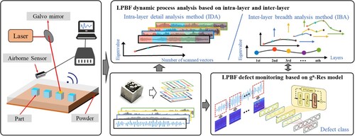
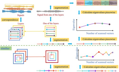
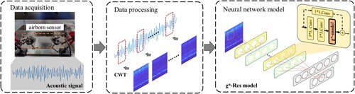
In this study, we have established a quantitative evaluation index derived from the pore distribution in microtopography images and the extent of deformation depressions present on the part's surface. This index serves to gauge the severity of defects and offers a foundation for the hierarchical categorisation of both pores and deformation defects. Secondly, this paper proposes a novel dynamic process analysis method of intra-layer to inter-layer acoustic properties, which can monitor the machining process in real time by tracking changes in statistical characteristics in units of scanning vectors. It can aid in exploring the typical characteristics of microscopic pores and macroscopic deformation defects. Based on the proposed method, the proportional relationship between the keyhole pores and the 38 k–42 kHz high-frequency component of the signal is established, providing guidance for sensor selection and accurate sensing. Finally, a novel gⁿ-Res-SC model is proposed to deeply mine process information through high-order interaction of spatial knowledge, achieving accurate identification of defects. The main structure of the article is shown in Figure 1.

Figure 1. The overview of the article.

2. LPBF experimental description

2.1. LPBF experiment

The experimental monitoring system, as illustrated in Figure 2a and b, comprises an LPBF system and an acoustic signal acquisition system. The LPBF system utilises a metal 3D printer (iSLM160), equipped with a fibre laser with a wavelength of 1064 nm, the maximum output power of the printer is 500 W, and the spot diameter ranges from 0.04 to 0.015 mm. The scan speed is 1.0–2.0 m/s.

Figure 2. LPBF acoustic signal monitoring system.

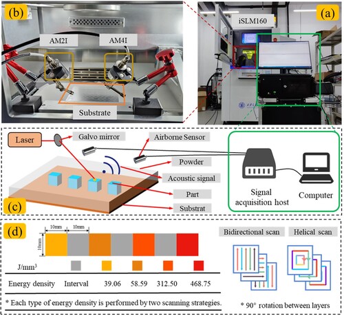
The acoustic signal acquisition system is equipped with two resonant airborne sensors (AM2I and AM4I) from the American PAC Company, which are positioned above the substrate at an angle of approximately 60° on its side. The airborne sensor uses a PCI sound signal data acquisition card and an IEIRACK305 acoustic emission host to connect to the PC for audio signal processing, and the sampling rate is set to 100 kHz. The experimental material was 316 L stainless steel powder, and the parts were arranged in the processing cabin in the positions shown in Figure 2c and d, and the scan speed of the laser in the interval is set to 800 mm/s.

The finished parts are shown in Figure 3, and their various processing parameters are shown in Table 1.

Figure 3. Characterisation of parts and their micromorphology.

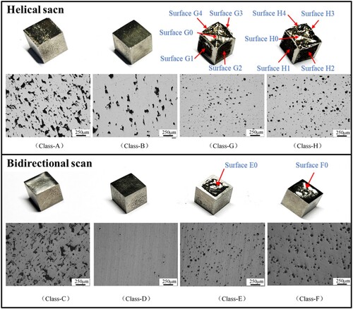
Table 1. Part processing parameters.

Class	Scan strategy	Scan power	Scan Speed	Scan line Spacing	Layer Thickness
A	Helical	100 W	800 mm/s	80 μm	40 μm
B	Helical	150 W	800 mm/s	80 μm	40 μm
C	Bidirectional	100 W	800 mm/s	80 μm	40 μm
D	Bidirectional	150 W	800 mm/s	80 μm	40 μm
E	Bidirectional	150 W	150 mm/s	80 μm	40 μm
F	Bidirectional	150 W	100 mm/s	80 μm	40 μm
G	Helical	150 W	150 mm/s	80 μm	40 μm
H	Helical	150 W	100 mm/s	80 μm	40 μm

It can be observed that Class-A, Class-B and Class-C mainly present irregular unfused morphology, with different severity, and large differences in unfused size and morphology. The reason for the unfused morphology is that due to insufficient energy input of some powders, the melt pool becomes smaller and the penetration depth is insufficient, so that the powder at the bottom of the melt pool is not fused. This may not only be directly caused by insufficient laser energy input, but also by frequent energy fluctuations in the helical scan strategy. The microscopic morphology of Class-D, Class-G, Class-H, Class-E and Class-F shows different shapes, including spherical, flat and other irregular-shaped keyhole pores.

The formation of keyhole defects is associated with the keyhole mode observed at high laser energy densities. As the energy density increases, the depth of the keyhole also increases. The keyhole exists in an unstable state, continuously expanding and contracting, while constantly changing its shape and depth. Additionally, there is a vigorous flow of liquid within the molten pool. Particularly when metal vapour inside the keyhole is expelled outward, it induces eddy currents within the keyhole that can easily draw in protective gas. With progression of the process, the position of the keyhole moves forward. When the tail end of the keyhole shrinks and collapses, bubbles are generated at its bottom. If these bubbles get trapped by solidification front during floating process, they remain in welds forming keyhole pores within them. Consequently, increasing laser energy density reduces or even eliminates unfused pores; however excessively high energy densities lead to generation of keyhole pores.

Deformation defects appear in Class-E, Class-F, Class-G and Class-H with higher laser energy density, mainly manifesting as concave distortion at the top of the part. There are also varying degrees of deformation around Class-G and Class-H parts. The top distortion is mainly due to the steep temperature gradient. During the laser melting process, the top powder material lacks the constraints of the surrounding materials. The heated top area begins to expand and form compressive stress, causing convex deformation. When a layer of powder scanning is completed, the cooling shrinkage of the heated area forms tensile stress, forming a concave distortion. The nature of the layered manufacturing method makes this process repeat, resulting in severe concave distortion. And for helical scan, the scanning path gradually decreases, which will lead to a large residual heat effect. The frequent changes in the scanning direction cause large changes in the temperature distribution, so that the degree of deformation is greater than that of bidirectional scan.

2.2. Offline quantitative characterisation of defects

Accurate evaluation of defect degrees is of great significance for analysing the source of defects and measuring product performance. Compared with qualitative evaluation of the degree of defects of Shevchik et al. [39] and Mohammadi et al. [46] when designing an LPBF defect monitoring system, this method can achieve quantitative evaluation of the degree of defects. For the preliminary results obtained by optical microscopes and optical measurement systems, software algorithms are used for secondary processing to obtain quantitative indicators that can measure the degree of defects.

For pore defects, computer vision is used to process microscopic images obtained by optical microscopy, as shown in Figure 4. Based on this, quantitative analysis indicators for measuring the degree of pores were proposed, including NP (Number of Pores), PS (Porosity, ratio of total pore area to image area), APS (Average Pore Size, ratio of total pore area to number), APP (Average Pore Perimeter, ratio of total pore perimeter to number). The results are shown in Table 2. Note that the area of the pore is the actual number of pixels in the pore area, and the perimeter of the pore is the distance between pairs of adjacent pixels at the boundary of the pore area.

Figure 4. Microscopic image processing process based on computer vision.

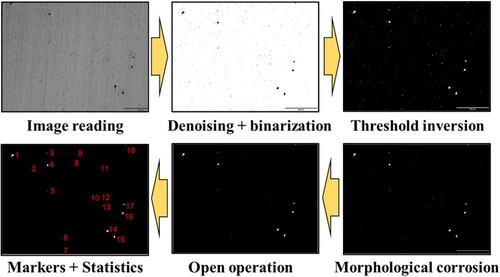
Table 2. Characterisation of pore defect categories and degrees.

Class	NP	PS	APS	APP	Defect definition
A	424	10.650%	1234.80	126.70	Heavily unfused pores (PS:10–15%)
B	116	5.086%	2151.47	166.98	Moderate unfused pores (PS:5–10%)
C	509	15.100%	1457.72	145.99	Severely unfused pores (PS:>15%)
D	21	0.069%	171.11	38.35	Seldom keyhole pores (PS:0–0.5%)
E	371	3.286%	432.13	68.30	Heavily keyhole pores (PS:3–5%)
F	443	5.071%	544.58	77.41	Severely keyhole pores (PS:>5%)
G	116	0.908%	395.67	64.09	Mild keyhole pores (PS:0.5–1%)
H	258	2.734%	523.79	73.03	Moderate keyhole pores (PS:1–3%)

The results are the average of all microscopic images of each type.

For macroscopic deformation defects, the optical fibre dispersion confocal three-dimensional measurement system is used to measure the degree of deformation, which can accurately measure microscopic deformation within 1 mm. As shown in Figure 4, the relevant deformation surfaces of the deformed parts are measured.

The degree of defect is defined by calculating the average deformation amount and maximum deformation amount of the deformation area within each deformation plane, as shown in Table 3. Note that the measurement points involved in the calculation are all located in the deformation area, that is to say, the measurement points in the non-deformation area are removed by using the algorithm. Secondly, for each measurement point, the result is processed as the amount of depression relative to the undeformed area within the scan line where it is located.

Table 3. Deformation defect characterisation.

Class		Max deformation	Mean deformation	Deformation
A/B/C/D		None	None	None
E	E0	467.90 μm	176.31 μm	Moderate
F	F0	801.39 μm	417.25 μm	Heavy
G	G0	>>1 mm	>>1 mm	Severely
	G1	660.76 μm	302.64 μm
	G2	894.04 μm	489.85 μm
	G3	784.06 μm	367.84 μm
	G4	589.01 μm	235.9 μm
H	H0	>>1 mm	>>1 mm	Severely
	H1	851.99 μm	320.73 μm
	H2	680.71 μm	315.15 μm
	H3	817.42 μm	395.81 μm
	H4	1129.80 μm	682.87 μm

Combining the defect characterisation results and processing parameters, scanning method and energy density are the main factors affecting the degree of part defects. For unfused pores, increasing energy density will reduce unfused pores. Compared with helical scan, bidirectional scan results in more unfused pores when the energy density is lower. When the energy density is increased, bidirectional scan presents better part quality. For keyhole pores, increasing energy density results in increased pores, while bidirectional scan results in more pores relative to helical scan.

3. LPBF dynamic process analysis based on intra-layer and inter-layer

3.1. Real-time analysis method based on statistical characteristics of scan vectors

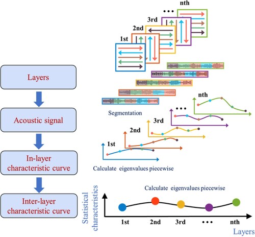
LPBF is a point-by-line manufacturing technology, so directly obtaining features from a layer of signals cannot reflect the changes within the layer. Directly obtaining features by violent segmentation of a layer of signals will lose the physical meaning of the information. In order to overcome this drawback, this paper proposes a real-time analysis method for the statistical characteristics of intra-layer and inter-layer scan vectors, including the intra-layer detail analysis method (IDA) and the inter-layer breadth analysis method (IBA). The IDA can analyse changes within the layer in detail, while the IBA can comprehensively analyse the overall processing status.

3.1.1. Intra-layer detail analysis method (IDA)

The IDA is shown in Figure 5. Different part sizes, scan line spacing and scan strategies result in different laser movement paths according to which the acoustic signals within the layer are segmented. This method can capture the acoustic wave signal corresponding to each scanning vector, and perform LPBF dynamic process analysis based on it.

Figure 5. Intra-layer detail analysis method (IDA) diagram.

During LPBF processing, the acoustic signal $x(t)$ can be expressed as: (1) $x(t)=[x_1(t),x_2(t),\dots ,x_n(t)]$(1) Where $n$ is the number of processing layers. For intra-layer signals $x_k(t),k\in [1,n]$, divide it into $p$ sequences according to the scan strategy. For the helical scan strategy, the number of scan vectors can be expressed as: (2) $p=C\times 4=\lfloor {\displaystyle \frac{L}{2\times l}+1}\rfloor \times 4$(2) Where $L$ is the side length of the part, $l$ is the scan line interval, $C$ represents the number of helical, and one helical number contains four scan vectors;

For bidirectional scan, the number of scan vectors can be expressed as: (3) $p=\lfloor {\displaystyle \frac{L}{l}+1}\rfloor$(3) For signal $x_k(t)$ within a layer, can be expressed as: (4) $x_k(t)=[x_k^1(t),x_k^2(t),\dots ,x_k^p(t)]$(4) Calculating the statistical characteristics of a single scan vector in a single layer signal can obtain the statistical feature sequence of the intra-layer processing status changing with the scan vector during the processing process: (5) $f_a(x_k(t))=[f_a(x_k^1(t)),f_a(x_k^2(t)),\dots ,f_a(x_k^p(t))]$(5) where $f_a$ is the intra-layer statistical feature calculation function, which can be time domain statistical features such as mean square value, variance, waveform factor, etc., or it can also be frequency domain features. Of course, it can also be a custom feature.

In this way, the intra-layer scan vector statistical characteristic curve is drawn with the scan vector $p$ as the independent variable and $f_a(x_k(t))$ as the dependent variable, which can represent the dynamic change of the processing state in a single layer following the scan vector.

3.1.2. Inter-layer breadth analysis method (IBA)

Based on IDA, the inter-layer breadth analysis method (IBA) is proposed, which can better observe the changes in the entire processing process. It analyses the entire processing process in terms of changes in the statistical characteristics of the scan vectors within a layer, combining the intra-layer changes with the global changes, which is implemented as shown in Figure 6.

Figure 6. Inter-layer breadth analysis method (IBA) diagram.

IDA can be used to obtain the statistical feature sequence of each layer signal that changes with the scan vector. Therefore, for the overall acoustic signal $x(t)=[x_1(t),x_2(t),\dots ,x_n(t)]$, the statistical feature change sequence within the $n$ layers can be expressed as (6) $f_a(x(t))=[f_a(x_1(t)),f_a(x_2(t)),\dots ,f_a(x_n(t))]$(6) For the statistical feature change sequence $f_a(x_k(t))$ of the k-th layer signal, its statistical feature can be calculated as$F_{\mathrm{b}}(f_a(x_k(t)))$, which measures the variation of the scan vector within the k-th layer. $F_{\mathrm{b}}$ is the inter-layer statistical feature calculation function.

For the overall processing signals$x(t)=[x_1(t),x_2(t),\dots ,x_n(t)]$, the change sequence of the statistical feature within the layer following the change of the number of layers can be obtained: (7) $F_{\mathrm{b}}(f_a(x(t)))=[F_{\mathrm{b}}(f_a(x_1(t))),F_{\mathrm{b}}(f_a(x_2(t))),\dots ,F_{\mathrm{b}}(f_a(x_n(t)))]$(7)

3.2. Time domain analysis of dynamic process of unfused pores based on IBA

In time domain, the IBA is used to conduct dynamic analysis of unfused pores, and the calculation function of the statistical feature quantity within the layer is defined as the mean square value: (8) $f_a(m(i))={\psi }_m^2(i)={\displaystyle \frac{1}{n}\sum _{i=1}^n{m}^2(i)=E(m^2(i))}$(8) where $m(i)$ is the acoustic signal corresponding to one of the scan vectors in a certain layer. Let the inter-layer statistical feature calculation function be the mean and variance, which can represent the distribution and changes of the signal: (9) $\{\begin{array}{c}{F}_{\mathrm{b}1}(n(j))={\displaystyle \frac{1}{p}\sum _{j=1}^{p}n(j)}\\ F_{\mathrm{b}2}(n(j))={\displaystyle \frac{1}{p}\sum _{j=1}^p{(n(j)-\overline{n})}^2}\end{array}$(9) where $n(i)$ is the statistical feature sequence of a certain layer, and $p$ is the number of scan vectors in a layer.

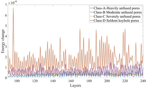
In order to ensure the reliability of the experimental results, the number of intermediate layers with stable processing processes was selected for analysis and processing. The dynamic change curves of the unfused pore process based on IBA are shown in Figures 7 and 8. It can be seen that in the case of unfused pores, the helical scan is more sensitive to changes in energy density than bidirectional scan. Under the same energy difference, the difference of dynamic change curves between Class-A and Class-B is much greater than that between Class-C and Class-D. Moreover, at lower energy densities, the energy distribution of Class-A is much smaller than that of Class-C, and the energy fluctuation is smaller than that of Class-C. After the energy density increases, the energy distribution of Class-B is smaller than Class-D, while the energy fluctuation is larger than Class-D. Secondly, the increase in energy density will lead to energy fluctuations, especially in helical scan, which is consistent with the characteristics of helical scan that continuously changes the length and direction of the scan vector. This results in a greater degree of unfused than bi-directional scan, and it is worth noting that Class-D has moved away from unfused porosity, while Class-B still exhibits unfused porosity.

Figure 7. Dynamic real-time analysis of unfused pore energy distribution based on IBA.

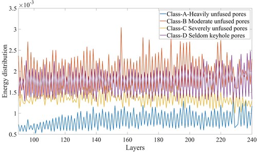
Figure 8. Dynamic real-time analysis of unfused pore energy fluctuation based on IBA.

3.3. Frequency domain analysis of keyhole pore dynamic process based on IBA

In frequency domain, the IBA is used to conduct dynamic real-time analysis of keyhole pores, and the calculation function of the statistical characteristic quantity within the layer is defined as: (10) $\{\begin{array}{c}{f}_a(m(i))=\mathrm{High}\mathrm{\_rate}(\mathrm{VMD}(m(i)))\\ \mathrm{High}\mathrm{\_rate}(c_v(i))={\displaystyle \frac{\mathrm{high}\mathrm{\_power}(c_v(i))}{\mathrm{all}\mathrm{\_power}(c_v(i))}}\\ \mathrm{all}\mathrm{\_power}(c_v(i))=\sum _{i=1}^N{|c_v(i)|}^2\\ \mathrm{high}\mathrm{\_power}(c_v(i))=\sum _{v=1}^N{|c_v(i)|}^2\mathrm{ifCen}\mathrm{\_Fre}(c_v(i))>R\end{array}$(10) where $f_a(m(i))$ is used to calculate the energy proportion of high-frequency signals in the signal. $m(i)$ is the acoustic signal corresponding to one of the scan vectors in a certain layer. VMD is the modal decomposition algorithm, which decomposes the signal into v Intrinsic Mode Functions $c_{\mathrm{v}}(i)$ with different frequency and amplitude characteristics [47]. $\mathrm{Cen}\mathrm{\_Fre}(c_{\mathrm{v}}(i))$ is used to calculate the centre frequency of $c_v(i)$. R is the frequency division threshold, which is 20 kHz by default. In the programme, scan vectors with a time length of less than 20 ms will not be computed because too short a signal length can cause distortion in the VDM decomposition results.

Let the inter-layer statistical feature calculation function be the mean value: (11) $F_{\mathrm{b}}(n(j))={\displaystyle \frac{1}{p}\sum _{j=1}^{p}n(j)}$(11) where $n(j)$is the sequence of statistical features of a layer and $p$ is the number of scan vectors within a layer.

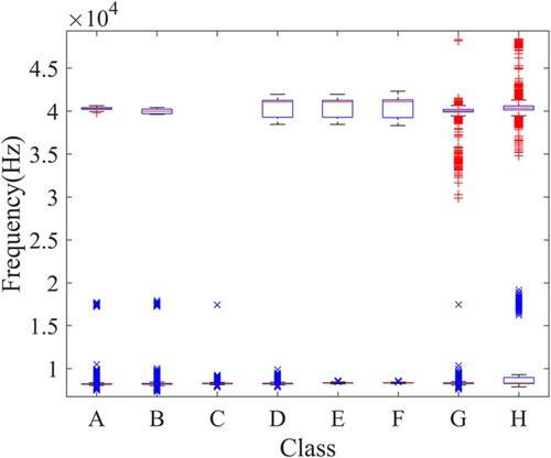
As shown in Figure 9, frequency components above 20 kHz are basically absent in the unfused pores, and high-frequency components are present only in the keyhole pores. Combined with the results in Figure 10, it can be seen that the higher the number of keyholes, the more high-frequency components, which is basically proportional to the relationship. Thus the keyhole pores bring in high-frequency components, which coincides with the discovery of the keyhole pore formation mechanism [48]. During the formation of a keyhole pore, the root of the keyhole is deformed in the form of a needle, which then expands explosively, releasing acoustic waves (shock waves) in the melt pool, thus leading to a high-frequency acoustic signal. Secondly, bidirectional scan leads to more high-frequency components, and an increase in energy density leads to an increase in high-frequency components, which is the same as the result of keyhole porosity characterisation. The frequency distribution of the centre of each mode for each scan vector throughout the machining process is counted. An energy threshold is designed so that only modes with an energy share of more than 30% are recorded, and the results are shown in Figure 11. The low-frequency components of unfused and keyhole pores are distributed in the range of 8 k to 8.5 kHz, and the high-frequency components of keyhole pores are distributed in the range of 38 k to 42 kHz. The helical scan has more abnormal points in this range, which may be due to anomalies caused by large energy fluctuations in the helical scan.

Figure 9. Dynamic real-time analysis of high-frequency percentage of pore defects.

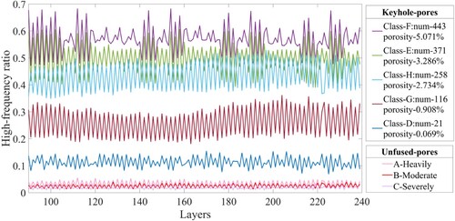
Figure 10. Correlation curve between number of keyholes and proportion of high frequency.

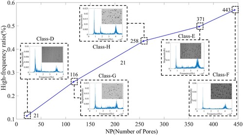
Figure 11. High and low frequency distribution interval.

3.4. Time domain analysis of deformation dynamic process based on IDA

For deformation defects, the Intra-layer detail analysis method is used to conduct dynamic real-time analysis of the deformation process, and the calculation function of the statistical feature within the layer is defined as the mean square value: (12) $f_a(m(i))={\psi }_m^2(i)={\displaystyle \frac{1}{n}\sum _{i=1}^n{m}^2(i)=E(m^2(i))}$(12)

Where $m(i)$ is the acoustic signal corresponding to one of the scan vectors in a certain layer.

As shown in Figure 12, severely deformation defects generally cause sudden changes in the energy of the acoustic signal during the later stages of the processing process. The Hilbert-Huang Transform (HHT) is used to obtain the instantaneous frequency changes during the entire machining process within the layer. It was found that the main frequency of the acoustic signal did not change during the machining process, but the number of excitations was greatly reduced. The time domain waveform of the acoustic signal confirmed this phenomenon.

Figure 12. Comprehensive analysis of deformation defect acoustic signal energy phenomenon.

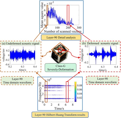
This phenomenon was not observed in the deformation induced by bidirectional scan, indicating that it is caused by the characteristics of helical scan. The outside-in scanning characteristic of helical scan causes large heat accumulation in the centre of the part. The large energy fluctuations cause the molten pool in the centre of the part to spatter, causing the surface of the part to be uneven. The uneven surface causes abnormal powder spreading, causing the laser to directly act on the moulding surface, resulting in a significant reduction in acoustic signals. In addition, the uneven surface and powder coating anomalies promote each other.

In summary, it should be noted that high energy input can induce part deformation, with scan strategy playing a crucial role in this regard. Deformation defects are primarily observed at elevated energy densities, and an increase in energy density leads to a higher degree of deformation, particularly when employing helical scan as opposed to bi-directional scan. During the LPBF process, the localised action of the high-energy laser beam results in rapid temperature distribution changes due to its swift movement, thereby causing significant alterations in the temperature gradient. Consequently, any modification in the scan strategy directly influences the temperature distribution throughout the LPBF process. Unlike direct application of energy density onto powder particles, altering the scan strategy allows for different cooling rates and heat treatment methods within specific processing areas by manipulating temperature distribution patterns. This aspect exerts a profound influence on stress and deformation distributions within LPBF-formed parts.

4. LPBF defect monitoring based on gⁿ-Res model

4.1. The proposed general process of LPBF online evaluation

The online evaluation of the LPBF process is implemented in this section using a deep learning algorithm. The implementation process is illustrated in Figure 13. Initially, airborne sensors and data acquisition devices are employed to capture acoustic signals during the processing stage. These signals are then segmented and processed using continuous wavelet transform to generate a time-frequency image dataset. Subsequently, by incorporating the concept of higher-order interaction into the residual network, we develop the gⁿ-Res model with enhanced feature extraction capabilities, enabling effective online evaluation of defects in the LPBF process.

Figure 13. LPBF Online Assessment Generic Process.

4.1.1. The preparation of the acoustic dataset

The above studies have well demonstrated that time-frequency features can effectively represent the process information of LPBF, so using time-frequency images as ML input is a higher choice. Wavelet transform can calculate the relative energy density of different frequency bands, so that it can express acoustic characteristics in frequency and time at the same time, which is very suitable for analysing non-stationary signals and extracting local features of signals.

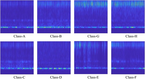
For the acoustic signal$x(t)\in L^2(R)$, its continuous wavelet transform is: (13) $W(\mathrm{a},\mathrm{b})={\displaystyle \frac{1}{\sqrt{a}}{\int }_{-\mathrm{\infty }}^{\mathrm{\infty }}x(t){\phi }^{\ast }({\displaystyle \frac{t-b}{a})\mathrm{dt}}}$(13) Where a is the scale factor, b is the time shift factor, and $\phi ({\displaystyle \frac{t-b}{a})}$ is the wavelet basis function. Figure 14 shows the wavelet transform results of the 100 ms segment from the acoustic signal of each category.

Figure 14. Time-frequency feature map of each class.

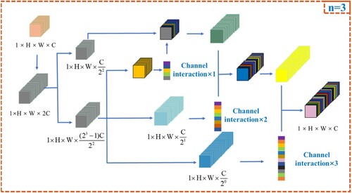
4.1.2. The proposed high-order interaction module

The high-order spatial interaction module uses the ideas of gating and recursion to realise high-order interaction of spatial information, but it ignores the information interaction in the channel. In order to better capture feature information, this work uses attention mechanism to help the model selectively focus on important information. Specifically, the channel attention operation is performed after the depth-separable convolution of spatial information is obtained, so that the perspective is focused on channels rich in spatial information.

Compared with the high-order spatial interaction module, gⁿ-SC integrates channel information before spatial interaction. The channel attention mechanism uses Efficient Channel Attention (ECA) [49]. The reason is that ECA uses 1 × 1 convolution to extract channel attention, and its receptive field is determined by the number of channels, which allows for optimal receptive fields for information sequences of different orders. It is worth mentioning that for different application scenarios, different channel attention can be used to implement different feature extraction operations.

Assume the input feature is $\mathrm{x}\in {\mathbb{R}}^{\mathrm{H}W\times C}$, and obtain a series of projection features ${\mathbf{p}}_0$ and $\{{\mathbf{q}}_h{\}}_{\mathrm{h}=0}^{\mathrm{n}\text{-}1}$ through ${\varphi }_{\mathrm{in}}$: (14) $[{\mathbf{p}}_0^{\mathrm{HW}\times C_0},{\mathbf{q}}_0^{\mathrm{HW}\times C_0},\dots ,{\mathbf{q}}_0^{\mathrm{HW}\times C_{n-1}}]={\varphi }_{\mathrm{in}}(x)\in {\mathbb{R}}^{\mathrm{HW}\times (C_0+{\sum }_{0\le k\le n-1}{C}_k)}$(14) where ${\varphi }_{\mathrm{in}}$ is a linear projection operation, which realises dimension conversion and dimension information exchange, and then performs gated convolution in a recursive manner: (15) ${\mathbf{p}}_{h+1}=f_h({\mathbf{q}}_h)\odot [\mathrm{att}(f_h({\mathbf{q}}_h))\times g_h({\mathbf{p}}_h)]/\alpha ,h=0,1,\dots ,n-1$(15) Where, $\{f_h\}$ is a set of deep convolutional layers; $\{\mathrm{att}\}$ is the channel attention mechanism. Different channel attention mechanisms are selected according to different data characteristics, and the ECA attention mechanism is selected. Note that ${\mathbf{p}}_{h+1}^{(i,c)}={\sum }_{j\in {\Omega }_i}{w}_{i\to j}^c{\mathbf{q}}_h^{(j,c)}{\mathbf{p}}_h^{(i,c)}$, where ${\Omega }_i$ is a local window centred at $i$ and $w$ represents the convolution weight of $f$. Therefore, the above formulation explicitly introduces interactions among the neighbouring features ${\mathbf{p}}_h^{(i)}$ and ${\mathbf{q}}_h^{(j)}$ through the element-wise multiplication.

In addition, the process of spatial interaction can be removed, channel information can be extracted directly, and an iterative channel attention operation gⁿ-CH can be implemented. Since spatial interaction is abandoned and the calculation of matrix multiplication is eliminated, the amount of calculation is greatly reduced, and only high-order interactions at the channel degree are performed recursively: (16) ${\mathbf{p}}_{h+1}=\mathrm{att}({\mathbf{q}}_h)\times g_h({\mathbf{p}}_h)/\alpha ,h=0,1,\dots ,n-1,$(16) Where, $\{\mathrm{att}\}$ is the channel attention mechanism, this article chooses to use the ECA.$\{g_k\}$ are used to match the dimension in different orders: (17) $g_h=\{\begin{array}{c}\mathrm{Identity},\mathrm{k}=0\\ \mathrm{Linear}({\mathrm{C}}_{\mathrm{h}\text{-}1},{\mathrm{C}}_h),1\le h\le n-1\end{array}$(17)

Finally, we feed the output of the last recursion step ${\mathbf{q}}_n$ to the projection layer ${\varphi }_{\mathrm{out}}$ to obtain the result of the gⁿ-SC or gⁿ-CH. (19) $y={\varphi }_{\mathrm{out}}({\mathrm{p}}_{\mathrm{n}})\in {\mathbb{R}}^{\mathrm{HW}\times C}$(19)

From the recursive formula Equations (14) or (15), it is easy to show that the interaction-order of ${\mathrm{p}}_{\mathrm{k}}$ will be increased by 1 after each step. To ensure that high-order interactions do not introduce too much computational overhead, the channel dimensions of each order $C_k$ are set to: (19) $C_h={\displaystyle \frac{C}{2^{n-h-1}},0\le h\le n-1}$(19)

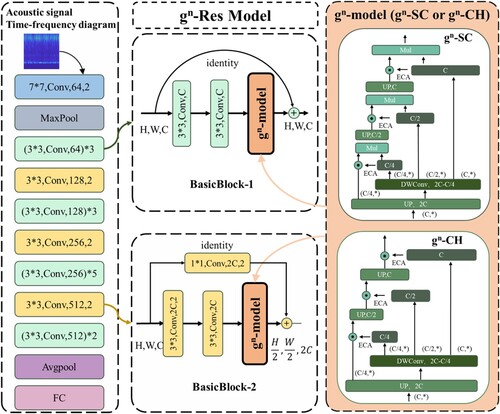
For the original implementation of high order spatial interaction, please refer to [45]. Through the above settings, we obtain the high-order information interaction module gⁿ-SC and the high-order channel interaction module gⁿ-CH. The third-order information interaction structure is shown in Figures 15 and 16.

Figure 15. Schematic diagram of gⁿ-SC structure.

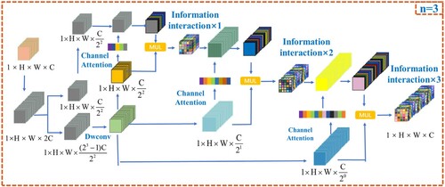
Figure 16. Schematic diagram of gⁿ-CH structure.

4.1.3. The proposed gⁿ-Res model

The improved high-order interaction module gⁿ-SC has more powerful feature extraction capabilities, but increases the complexity of the network. This effect is particularly pronounced within the HorNet network architecture due to its deeper and more intricate structure. This paper combines the gⁿ-SC module with the residual structure and designs the gⁿ-Res model, its network structure is shown in Figure 17. The residual structure jump connection can effectively solve the problem of performance degradation caused by too deep a network [50].

Figure 17. gⁿ-Res model structure.

4.2. Model evaluations

The performance of the proposed method is evaluated from four aspects: accuracy, precision, recall and F1 score, as shown in Table 4. All comparison methods were implemented based on Pytorch and Python, and the experiments were run on a server equipped with NVIDIA GeForce RTX 3090. The model parameters are shown in Table 5.

Table 4. Model performance metrics.

Metrics	Equations	Notes
Accuracy	${\displaystyle \frac{\mathrm{TP}+\mathrm{TN}}{\mathrm{TP}+\mathrm{TN}+\mathrm{FP}+\mathrm{FN}}}$	/
Precision	${\displaystyle \frac{\mathrm{TP}}{\mathrm{TP}+\mathrm{FP}}}$	Positive Predicted Value (PPV)
Recall	${\displaystyle \frac{\mathrm{TP}}{\mathrm{TP}+\mathrm{FN}}}$	True Positive Rate (TPR) or Sensitivity
F1-score	$2\times {\displaystyle \frac{\mathrm{Precision}\times \mathrm{Recall}}{\mathrm{Precision}+\mathrm{Recall}}}$	Harmonic mean of Precision and Recall

Note: TP, FN, TN and FP represent true positive, false negative, true negative and false positive respectively.

Table 5. Parameters used for the model.

Training parameters	Model
Training objective	Classification
Rate of learning	0.001
Optimizer used	Adam
Total epochs	100
Training batch size	128
Shuffle	Ture
Loss	Cross-entropy loss
Train dataset	19,200(2400/class)
Validation dataset	4800(600/class)
Test dataset	4000(500/class)

4.2.1. Effectiveness analysis of high-order interactive modules

Due to the layer-by-layer processing characteristics of LPBF, the acoustic signals in the middle and later stages of processing encapsulate physical information from preceding layers. The intricate intertwining of spatial and temporal scales gives rise to highly abstract features. Leveraging the concept of high-order interaction can facilitate more effective extraction of underlying information.

In order to verify its effectiveness, the gⁿ-SC and gⁿ-CH modules were embedded into the original framework HorNet, and their performance was compared using the time-frequency dataset. The results are presented in Table 6. The results are presented in Table 6. It is evident that the performance of HorNet_SC with incorporated channel information surpasses that of the original framework significantly. Although HorNet uses high-order spatial interaction to greatly improve feature extraction capabilities, its implementation involves complex channel settings, so HorNet_SC with added channel information can better achieve information flow. The performance of HorNet_CH is similar to that of the original framework, but gⁿ-CH removes matrix multiplication and has more advantages in terms of calculation amount.

Table 6. Performance comparison of high-order interactive modules.

Models	Auracy_score	Precision_score	Recall_score	F1_score
HorNet	81.97%	84.36%	81.97%	81.48%
HorNet_CH	82.25%	82.98%	82.25%	81.68%
HorNet_SC	87.65%	88.80%	87.65%	87.33%

HorNet_SC with high-order space and channel interaction has powerful feature extraction capabilities, but it also increases the complexity of the network. The complexity of HorNet_SC, which is combined with complex feature extraction architecture of HorNet, has been greatly increased. The stacked gⁿ-SC modules have resulted in a larger network depth, which has not achieved the expected performance.

4.2.2. Comparison with the state of the arts approach

To evaluate the proposed model, other popular attention modules are replaced with the proposed network to analyse their performance changes, including SE-Net [51], CMBA [52] and ECA; and Other CNN and RNN network architectures, including AlexNet [53], Vision Transformer [54], Efficientnet [55], GRU [56] and LSTM [57]. Secondly, the models based on one-dimensional features are compared, such as the Support Vector Machine (SVM) and Artificial Neural Network (ANN). The construction of one-dimensional features is based on the research of [58].

From the performance comparison shown in Table 7, it can be found that the realisation of GRU and LSTM is not outstanding, and all the information of the processing process cannot be fully obtained through Timing characteristics alone. This is to be expected, because due to the layer-by-line processing characteristics of LPBF, feature information is often more relevant to space. The performance of AlexNet, Efficientnet and ViT is also unsatisfactory. By increasing the complexity and depth of the network, the LPBF process information cannot be effectively extracted, and better feature extraction methods are needed. The addition of attention mechanism can greatly improve the feature extraction ability of the network. Res_HorNet is far ahead in precision, which combines the high-order spatial interaction ideas of HorNet. And the improved information high-order interaction module gⁿ-Res_SC performs best in accuracy, recall and F1 scores. This shows that the high-order interaction method can fully extract highly abstract LPBF process information. It can be seen through the poor performance of Res_SE, Res_ECA and Res_CMBA. What is surprising is the performance of gⁿ-Res_CH. Compared with gⁿ-Res_SC, it reduces the amount of calculation, but the performance is only slightly reduced.

Table 7. Network performance comparison.

Models	Auracy score	Precision score	Recall score	F1 score
ANN	47.20%	52.19%	47.20%	43.49%
SVM	42.08%	42.35%	42.08%	41.97%
GRU	76.08%	77.31%	76.08%	73.50%
LSTM	72.75%	72.88%	72.75%	70.78%
AlexNet	81.20%	85.58%	81.20%	80.36%
VGG	88.35%	90.14%	88.35%	87.72%
ViT	87.60%	89.32%	87.60%	87.18%
Efficientnet	87.15%	89.40%	87.15%	87.18%
Res_SE	88.10%	89.80%	88.10%	87.99%
Res_ECA	89.98%	91.88%	89.98%	89.88%
Res_CMBA	89.83%	91.80%	89.83%	89.73%
Res_HorNet	90.17%	92.1%	90.17%	90.05%
g^n-Res_CH	90.47%	91.15%	90.17%	90.10%
g^n-Res_SC	90.70%	91.50%	90.70%	90.40%

It is worth noting that Res_HorNet has a very high precision (the proportion of correct predictions that are positive to all predictions that are positive), which is an important indicator for real-time monitoring of defects. Because predicting a critical defect as minor may result in the system continuing to operate without interruption or correction. However, gⁿ-Res_SC adds channel information on its basis and does not inherit its performance in precision. This may be due to the fact that the original spatial information is affected when the channel information is adjusted. Therefore, how to adjust channel information while retaining the original spatial information will be a future research direction.

At the same time, the model can realise defect identification in the LPBF process with an accuracy of 90.70% in a 100 ms window. It is worth noting that the selection of the segmentation length of 100 ms is a balance of the LPBF process under different processing parameters. Due to the difference in scan speed under the same sampling rate, the scan time of the laser per unit length is different. This results in different acoustic signal lengths under different processing parameters. Therefore, we truncated the acoustic signals under each class into 100 ms acoustic signal segments, and selected 3500 acoustic signal segments under each class of processing conditions in a random sampling manner to generate time-frequency images. In other words, we only used part of the data. Generally, a longer acoustic signal can provide more information about the acoustic signal, thereby improving the accuracy of the intelligent model. Choosing a window of 100 ms ensures the same information input to the intelligent model in different categories, while providing better spatiotemporal resolution. The model deeply mines the spatial information of LPBF through high-order spatial interaction, but does not explicitly utilise spatial information. The physical interpretability of the model needs to be further developed, which is the focus of the next step of research.

5. Conclusion

This paper obtained components with complex defects through variable parameter experiments, dynamically analysed the changing rules of acoustic signals based on the intra-layer-inter-layer feature analysis method, and finally achieved on-line evaluation of defects. The following conclusions can be drawn:

1. Insufficient energy density leads to unfused pores, but too high energy density leads to keyhole pores and deformation defects, and helical scan is more sensitive to changes in energy density, with greater energy fluctuations leading to more severe deformation, while bidirectional scan leads to more keyhole pores.

2. High frequency acoustic signals of 38 k–42 kHz are generated by keyhole pores, and the proportion of high frequency energy in the acoustic signals is proportional to the number of keyhole pores.

3. For the components with both different degrees of pores and deformation defects, gⁿ-Res_SC based on higher-order interactions is able to better extract the spatial information of the LPBF process, which is better than the current SOTA method in terms of accuracy (90.70%), recall (90.70) and F1-score (90.40%) on the test results on the acoustic time-frequency dataset.

However, the proposed LPBF process analysis method relies on the scan strategy to realise the segmentation of acoustic signals, which means that the corresponding acoustic signal segmentation algorithms need to be implemented in the face of different scan strategies, which will undoubtedly cost more time as well as labour costs, hindering the application of this method. Future research will focus on acoustic signal segmentation algorithms applicable to different scan strategies. And the research based on cubic parts ignores the changes in build performance and signal response caused by complex structural parts. When faced with defects caused by different geometric structures, the generalisation ability of the model needs further study. Secondly, the model achieves real-time monitoring of defects by mining the underlying information of AE signals, but it is not intuitive compared to video input, which can explicitly relate component performance in greater depth [59]. Finally, this study utilised random sampling to solve the problem of the difference in the amount of data generated under different processing parameters, but it also produced a waste of data. Therefore, solving the problem of acoustic signal length difference caused by scan speed is also one of the future research focuses.

CRediT authorship contribution statement

Shuai Zhang: Data curation, Software, Supervision, Writing – original draft, Writing – review & editing. Zhifen Zhang: Conceptualisation, Funding acquisition, Investigation, Writing – original draft. Rui Qin: Methodology, Supervision, Writing – original draft. Jie Wang: Data curation, Supervision. Zijian Bai: Data curation, Supervision. Zhiwen Li: Data curation, Supervision. Jing Huang: Data curation, Supervision. Guangrui Wen: Conceptualisation, Funding acquisition. Xuefeng Chen: Supervision, Validation.

Disclosure statement

No potential conflict of interest was reported by the author(s).

Data availability statement

The raw/processed data required to reproduce these findings cannot be shared at this time as the data also forms part of an ongoing study.

Additional information

Funding

This research is supported by the National Key R&D Program of China (No. 2022YFB4600800).

References

- Kruth J-P, Badrossamay M, Yasa E, et al. Part and material properties in selective laser melting of metals. Paper presented at: Proceedings of the 16th International Symposium on Electromachining (ISEM XVI); 2010.
- Frazier WE. Metal additive manufacturing: a review. J Mater Eng Perform. 2014;23(6):1917–1928. doi:10.1007/s11665-014-0958-z
- Jiaoxi Y, Wenliang W, Changliang W, et al. Development status and typical application of selective laser melting technology applications in aerospace field. 航空材料学报. 2021;41(2):1–15.
- Ataee A, Li Y, Brandt M, et al. Ultrahigh-strength titanium gyroid scaffolds manufactured by selective laser melting (SLM) for bone implant applications. Acta Mater. 2018;158:354–368. doi:10.1016/j.actamat.2018.08.005
- Vasco JC. Additive manufacturing for the automotive industry. In: Pou J, Riveiro A, Paulo Davim J, editors. Additive manufacturing. Elsevier; 2021. p. 505–530.
- Trapp J, Rubenchik AM, Guss G, et al. In situ absorptivity measurements of metallic powders during laser powder-bed fusion additive manufacturing. Appl Mater Today. 2017;9:341–349. doi:10.1016/j.apmt.2017.08.006
- Acharya R, Sharon JA, Staroselsky A. Prediction of microstructure in laser powder bed fusion process. Acta Mater. 2017;124:360–371. doi:10.1016/j.actamat.2016.11.018
- King WE, Barth HD, Castillo VM, et al. Observation of keyhole-mode laser melting in laser powder-bed fusion additive manufacturing. J Mater Process Technol. 2014;214(12):2915–2925. doi:10.1016/j.jmatprotec.2014.06.005
- Du Y, Arnold CB. Powder melting efficiency during laser powder bed fusion of stainless steel and titanium alloy. J Manuf Process. 2024;120:161–169. doi:10.1016/j.jmapro.2024.04.046
- Chua C, Liu Y, Williams RJ, et al. In-process and post-process strategies for part quality assessment in metal powder bed fusion: a review. J Manuf Syst. 2024;73:75–105. doi:10.1016/j.jmsy.2024.01.004
- Forien J-B, Calta NP, DePond PJ, et al. Detecting keyhole pore defects and monitoring process signatures during laser powder bed fusion: a correlation between in situ pyrometry and ex situ X-ray radiography. Addit Manuf. 2020;35:101336. doi:10.1016/j.addma.2020.101336
- Guo C, Xu Z, Zhou Y, et al. Single-track investigation of IN738LC superalloy fabricated by laser powder bed fusion: track morphology, bead characteristics and part quality. J Mater Process Technol. 2021;290:117000. doi:10.1016/j.jmatprotec.2020.117000
- Du C, Zhao Y, Jiang J, et al. Pore defects in laser powder bed fusion: formation mechanism, control method, and perspectives. J Alloys Compd. 2023;944:169215. doi:10.1016/j.jallcom.2023.169215
- Leuders S, Thöne M, Riemer A, et al. On the mechanical behaviour of titanium alloy TiAl6V4 manufactured by selective laser melting: fatigue resistance and crack growth performance. Int J Fatigue. 2013;48:300–307. doi:10.1016/j.ijfatigue.2012.11.011
- Hojjatzadeh SMH, Parab ND, Guo Q, et al. Direct observation of pore formation mechanisms during LPBF additive manufacturing process and high energy density laser welding. Int J Mach Tools Manuf. 2020;153:103555. doi:10.1016/j.ijmachtools.2020.103555
- Fatemi A, Molaei R, Sharifimehr S, et al. Multiaxial fatigue behavior of wrought and additive manufactured Ti-6Al-4 V including surface finish effect. Int J Fatigue. 2017;100:347–366. doi:10.1016/j.ijfatigue.2017.03.044
- Jost EW, Miers JC, Robbins A, et al. Effects of spatial energy distribution-induced porosity on mechanical properties of laser powder bed fusion 316L stainless steel. Addit Manuf. 2021;39:101875. doi:10.1016/j.addma.2021.101875
- Krakhmalev P, Fredriksson G, Yadroitsava I, et al. Deformation behavior and microstructure of Ti6Al4 V manufactured by SLM. Phys Procedia. 2016;83:778–788. doi:10.1016/j.phpro.2016.08.080
- Everton SK, Hirsch M, Stravroulakis P, et al. Review of in-situ process monitoring and in-situ metrology for metal additive manufacturing. Mater Des. 2016;95:431–445. doi:10.1016/j.matdes.2016.01.099
- Clijsters S, Craeghs T, Buls S, et al. In situ quality control of the selective laser melting process using a high-speed, real-time melt pool monitoring system. Int J Adv Manuf Technol. 2014;75(5-8):1089–1101. doi:10.1007/s00170-014-6214-8
- Kanko JA, Sibley AP, Fraser JM. In situ morphology-based defect detection of selective laser melting through inline coherent imaging. J Mater Process Technol. 2016;231:488–500. doi:10.1016/j.jmatprotec.2015.12.024
- Grasso M, Colosimo BM. Process defects and in situ monitoring methods in metal powder bed fusion: a review. Meas Sci Technol. 2017;28(4):044005. doi:10.1088/1361-6501/aa5c4f
- Zur Jacobsmühlen J, Kleszczynski S, Schneider D, et al. High resolution imaging for inspection of laser beam melting systems. Paper presented at: 2013 IEEE international instrumentation and measurement technology conference (I2MTC); 2013.
- Chen L, Yao X, Tan C, et al. In-situ crack and keyhole pore detection in laser directed energy deposition through acoustic signal and deep learning. Addit Manuf. 2023;69:103547. doi:10.1016/j.addma.2023.103547
- Zhang L, Attar H. Selective laser melting of titanium alloys and titanium matrix composites for biomedical applications: a review. Adv Eng Mater. 2016;18(4):463–475. doi:10.1002/adem.201500419
- Thijs L, Verhaeghe F, Craeghs T, et al. A study of the microstructural evolution during selective laser melting of Ti–6Al–4 V. Acta Mater. 2010;58(9):3303–3312. doi:10.1016/j.actamat.2010.02.004
- Mercelis P, Kruth J. Residual stresses in selective laser sintering and selective laser melting. Rapid Prototyp J. 2006;12(5):254–265. doi:10.1108/13552540610707013
- Jia H, Sun H, Wang H, et al. Scanning strategy in selective laser melting (SLM): a review. Int J Adv Manuf Technol. 2021;113(9-10):2413–2435. doi:10.1007/s00170-021-06810-3
- Sames WJ, List FA, Pannala S, et al. The metallurgy and processing science of metal additive manufacturing. Int Mater Rev. 2016;61(5):315–360. doi:10.1080/09506608.2015.1116649
- Bartlett JL, Li X. An overview of residual stresses in metal powder bed fusion. Addit Manuf. 2019;27:131–149. doi:10.1016/j.addma.2019.02.020
- Wang Q, Jia J, Zhao Y, et al. In situ measurement of full-field deformation for arc-based directed energy deposition via digital image correlation technology. Addit Manuf. 2023;72:103635. doi:10.1016/j.addma.2023.103635
- Shevchik SA, Kenel C, Leinenbach C, et al. Acoustic emission for in situ quality monitoring in additive manufacturing using spectral convolutional neural networks. Addit Manuf. 2018;21:598–604. doi:10.1016/j.addma.2017.11.012
- Pandiyan V, Wróbel R, Richter RA, et al. Monitoring of laser powder bed fusion process by bridging dissimilar process maps using deep learning-based domain adaptation on acoustic emissions. Addit Manuf. 2024;80:103974. doi:10.1016/j.addma.2024.103974
- Pandiyan V, Drissi-Daoudi R, Shevchik S, et al. Analysis of time, frequency and time-frequency domain features from acoustic emissions during laser powder-bed fusion process. Procedia CIRP. 2020;94:392–397. doi:10.1016/j.procir.2020.09.152
- Ye D, Zhang Y, Zhu K, et al. Characterization of acoustic signals during a direct metal laser sintering process; 2017. p. 1315–1320.
- Ye D, Hong GS, Zhang Y, et al. Defect detection in selective laser melting technology by acoustic signals with deep belief networks. Int J Adv Manuf Technol. 2018;96(5-8):2791–2801. doi:10.1007/s00170-018-1728-0
- Pandiyan V, Wróbel R, Leinenbach C, et al. Optimizing in-situ monitoring for laser powder bed fusion process: deciphering acoustic emission and sensor sensitivity with explainable machine learning. J Mater Process Technol. 2023;321:118144. doi:10.1016/j.jmatprotec.2023.118144
- Pandiyan V, Wróbel R, Richter RA, et al. Self-Supervised Bayesian representation learning of acoustic emissions from laser powder bed fusion process for in-situ monitoring. Mater Des. 2023;235:112458. doi:10.1016/j.matdes.2023.112458
- Shevchik SA, Masinelli G, Kenel C, et al. Deep learning for in situ and real-time quality monitoring in additive manufacturing using acoustic emission. IEEE Trans Ind Inf. 2019;15(9):5194–5203. doi:10.1109/TII.2019.2910524
- Babu SS, Mourad A-HI, Harib KH, et al. Recent developments in the application of machine-learning towards accelerated predictive multiscale design and additive manufacturing. Virtual Phys Prototyp. 2022;18(1):e2141653. doi:10.1080/17452759.2022.2141653
- Zhang J, Yin C, Xu Y, et al. Machine learning applications for quality improvement in laser powder bed fusion: a state-of-the-art review. Int J AI Mater Design. 2024;1(1):2301. doi:10.36922/ijamd.2301
- Goh GD, Huang X, Huang S, et al. Data imputation strategies for process optimization of laser powder bed fusion of Ti6Al4 V using machine learning. Mater Sci Addit Manuf. 2023;2(1):50. doi:10.36922/msam.50
- Nguyen NV, Hum AJW, Do T, et al. Semi-supervised machine learning of optical in-situ monitoring data for anomaly detection in laser powder bed fusion. Virtual Phys Prototyp. 2023;18(1):e2129396. doi:10.1080/17452759.2022.2129396
- Vaswani A, Shazeer N, Parmar N, et al. Attention is all you need. Adv Neural Inf Process Syst. 2017;30:5998–6008.
- Rao Y, Zhao W, Tang Y, et al. Hornet: efficient high-order spatial interactions with recursive gated convolutions. Adv Neural Inf Process Syst. 2022;35:10353–10366.
- Mohammadi MG, Mahmoud D, Elbestawi M. On the application of machine learning for defect detection in L-PBF additive manufacturing. Opt Laser Technol. 2021;143:107338. doi:10.1016/j.optlastec.2021.107338
- Dragomiretskiy K, Zosso D. Variational mode decomposition. IEEE Trans Signal Process. 2013;62(3):531–544. doi:10.1109/TSP.2013.2288675
- Zhao C, Parab ND, Li X, et al. Critical instability at moving keyhole tip generates porosity in laser melting. Science. 2020;370(6520):1080–1086. doi:10.1126/science.abd1587
- Wang Q, Wu B, Zhu P, et al. ECA-net: efficient channel attention for deep convolutional neural networks. Paper presented at: Proceedings of the IEEE/CVF conference on computer vision and pattern recognition; 2020.
- He K, Zhang X, Ren S, et al. Deep residual learning for image recognition. Paper presented at: Proceedings of the IEEE conference on computer vision and pattern recognition; 2016.
- Hu J, Shen L, Albanie S, et al. Gather-excite: exploiting feature context in convolutional neural networks. Adv Neural Inf Process Syst. 2018;31:9423–9433.
- Woo S, Park J, Lee J-Y, et al. Cbam: convolutional block attention module. Paper presented at: Proceedings of the European conference on computer vision (ECCV); 2018.
- Krizhevsky A, Sutskever I, Hinton GE. Imagenet classification with deep convolutional neural networks. Adv Neural Inf Process Syst. 2012;25:1097–1105.
- Dosovitskiy A, Beyer L, Kolesnikov A, et al. An image is worth 16 × 16 words: transformers for image recognition at scale. Preprint, arXiv:2010.11929; 2020.
- Tan M, Le Q. Efficientnet: rethinking model scaling for convolutional neural networks. Paper presented at the International conference on machine learning; 2019.
- Cho K, Van Merriënboer B, Gulcehre C, et al. Learning phrase representations using RNN encoder-decoder for statistical machine translation. Preprint, arXiv:1406.1078; 2014.
- Hochreiter S, Schmidhuber J. Long short-term memory. Neural Comput. 1997;9(8):1735–1780. doi:10.1162/neco.1997.9.8.1735
- Guo L, Li N, Jia F, et al. A recurrent neural network based health indicator for remaining useful life prediction of bearings. Neurocomputing. 2017;240:98–109. doi:10.1016/j.neucom.2017.02.045
- Williams RJ, Sing SL. Spatiotemporal analysis of powder bed fusion melt pool monitoring videos using deep learning. J Intell Manuf. 2024:1–14. doi:10.1007/s10845-024-02355-w