Using satellite imagery to estimate heavy vehicle volume for ecological injury analysis in India

Abstract

A major limitation of road injury research in low- and-middle income countries is the lack of consistent data across the settings, such as traffic counts, to measure traffic risk. This study presents a novel method in which traffic volume of heavy vehicles – trucks and buses – is estimated by identifying these vehicles from satellite imagery of Google Earth. For Rajasthan state in India, a total of ∼44,000 such vehicles were manually identified and geo-located on national highways (NHs), with no distinction made between trucks and buses. To estimate population living in proximity to NHs, defined as those living within 1 km buffer of NH, we geocoded ∼45,000 villages and ∼300 cities using Google Maps Geocoding Application Programming Interface (API). We fitted a spatio-temporal Bayesian regression model with the number of road deaths at the district level as the outcome variable. We found a strong Pearson correlation of 0.84 (p < 0.001) between Google Earth estimates of heavy vehicles and freight vehicle counts reported by a national-level study for different road sections. The regression results show that the volume of heavy vehicles and rural population in proximity to highways are positively associated with fatality risk in the districts. These effects have been estimated after controlling for other modes of travel.

Keywords:

• Heavy vehicles
• google earth
• GIS
• traffic fatalities
• India
• ecological analysis

1. Introduction

India has suffered a nearly continuous growth of road fatalities over the past few decades. Over the 25-year period from 1980 to 2015, the number of road deaths grew 17 times, while the death rate rose 6 times, from 2.1 to 12 per 100,000 persons (MoRTH, 2017; NCRB, 2015). The analyses of crash-level data in various settings of India have shown that the buses and trucks are involved in 50–75% of fatal crashes on highways and 40% to 52% in the cities (Mohan et al., 2016; Naqvi & Tiwari, 2017). These shares are much higher than their share in total vehicles registered (∼5%), though it is likely that travel distance per vehicle is much greater than for cars and motorized two-wheelers (Goel et al., 2016; Malik & Tiwari, 2017). In case of a crash, buses and trucks also have greater likelihood than cars to result in fatality, because of their much higher weight as well as the design of vehicle front (Desapriya et al., 2010; Paulozzi, 2005). Freight movement in India is also dominated by on-road modes, with up to 60% of the freight mass transported on roads (RITES, 2014). The movement of trucks is strongly linked with the economy (Dhar & Shukla, 2015; Tiwari & Gulati, 2013), which has been rapidly growing in India during this period. With a focus on constructing new highways and widening the existing ones, the propensity of freight to use the road is likely to increase even further (Datta, 2012).

Given the strong evidence indicating heavy vehicle volume as a strong risk factor of road deaths in India and high likelihood of this volume to grow in the future, epidemiological research of traffic crashes needs to develop methods so that this risk factor can be adequately measured. Traffic volume is the traditional variable accounting for risk in accident prediction models (Elvik, 2011). However, data on freight movement in India are scarce. Vehicle-classified counts are usually conducted for a specific purpose such as planning a new road infrastructure, are restricted to a few locations, and often not in the public domain. Lack of any systematic efforts in traffic volume counts results in poor comparability across the settings. Vehicle registration data for freight vehicles can be misleading as their trips often span across multiple jurisdictions. For instance, in India, average distance travelled by on-road freight vehicles from origin to destination is 300 km (RITES, 2013). Censuses and travel surveys report data on passenger travel and have often been used in area-level accident prediction models (Aldred et al., 2018; Goel, 2018; Schepers & Heinen, 2013). However, these data sources lack any information on freight movement. Absence of a variable representing freight can potentially bring omitted-variable bias in the model results and significantly modify the effects of other variables (Mitra & Washington, 2012). For instance, in Goel (2018), effect of motorized two-wheelers on traffic fatality risk was overestimated by 70% when heavy-vehicle traffic measure was not accounted for in the model.

Researchers have successfully used commonly available geospatial data sources to fill data gaps in settings with lack of GIS data on built environment. In Goel et al. (2018), Google Earth and Google Maps were used to geocode the locations of traffic built-environment such as grade separated junctions, bus stops and traffic lights, as well as for mapping of built-up area. Further, satellite imagery has been used for mapping environmental variables for epidemiology of vector-borne diseases (Chang et al., 2009). Satellite images can also be used to detect traffic on the roads. There is a growing literature on developing machine learning methods for automatic detection of traffic using satellite imagery (Cao et al., 2016; Eikvil et al., 2009; Larsen et al., 2013; Tang et al., 2017). However, in these studies, there is much more focus on improving detection rates by the algorithms. Few studies have compared satellite-based estimation of traffic counts with ground-based data (Eikvil et al., 2009), and fewer still have shown application of such methods in the context of transportation research.

In this paper, we aim to test the use of widely accessible geospatial data sources to overcome the lack of data availability for road injury epidemiology in a low-income setting. We present the novel use of Google Earth satellite imagery to estimate heavy vehicle volume on highways for road safety epidemiology. To account for the population exposure to traffic injury risk, we present the use of Google Maps Application Programming Interface (API) for large-scale mapping of villages and towns. This will further demonstrate the use of a novel method to facilitate the development of geospatial dataset often unavailable in low- and -middle income settings (Hamilton et al., 2018). Finally, we present an ecological model using spatial regression methods to assess the relationship between road deaths and heavy vehicle volume.

2. Data and method

The study setting is Rajasthan, the north-western state of India (Figure 1). Geographically it is the largest state in India. In 2011, the state had a population of 68.6 million which is similar to that of France or the United Kingdom. Its surface area (3,42,000 km²) is comparable to that of Germany. Through road and rail, the state connects Delhi to its north-east, the capital city and an important commercial and industrial hub, with the seaports of Mumbai and Jawaharlal Nehru port (JNPT) on the western coast, and the latter is the largest container port in India. The state is also a major tourist destination with more than 30 million tourists per year (Rajasthan Tourism Department, 2014). The western half of the state, bordering Pakistan, is low-density desert region while the eastern half is where most population resides.

Figure 1. Map of India and location of Rajasthan state (top left), districts and national highway network with district census IDs in ellipses (bottom left) and 6-year average (and 95% confidence interval) of road death rates of the districts (right).

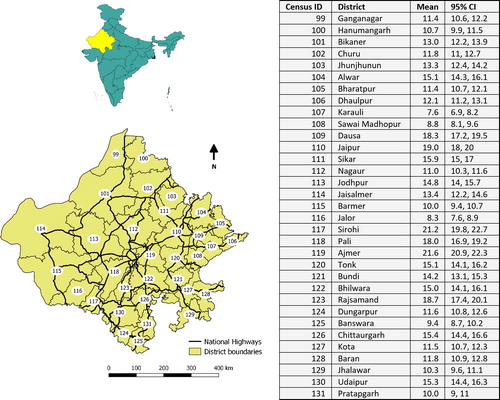
The aerial units of analysis are the 33 districts that represent administrative divisions within the state, and are comparable to counties in many countries. We used district-level number of road deaths from 2011 to 2016 reported by state police on their website (http://police.rajasthan.gov.in/default.aspx). Over the 6-year period, annual road deaths across the state increased from 9232 to 10,465. In 2011, the death rate of the state was 13.5 per 100,000 persons compared with country-wide rate of 11.3, and it is one of the 10 states with the highest death rates in India (Mohan et al., 2016). We used district-level population from 2001 and 2011 Censuses to estimate population of each district from 2012 through 2016 using linear extrapolation. For each district, the average death rates and 95% confidence interval (CI) using Poisson distribution over the 6-year period are presented in Figure 1. The rate varies from 7.7 deaths per 100,000 persons to more than 21 deaths per 100,000 persons in two districts.

In the 2011 Census of India, mode of travel to work was reported for workers (Census-India, 2017). We used the number of workers travelling to work by different modes in each district to represent passenger travel patterns. The different modes included in this analysis are walk, cycle, motorized two-wheelers (m2w), car, intermediate public transport (ipt) modes such as three-wheeled auto rickshaws or tuk-tuks (Kumar et al., 2016), bus and train. Table 1 presents the descriptive statistics of all the variables.

Table 1. Descriptive statistics of study variables for 33 districts.

Variable name	Description		Mean	Standard deviation	Median	Minimum	Maximum
deaths	Annual number of deaths		302	228	241	70	1446
population	Population of district		2,157,713	1,168,779	1,968,516	672,008	7,289,051
walk commuters	Number of commuters travelling to work by	Walking	81,800	48,401	69,083	25,896	301,476
cycle commuters		Cycling	28,910	24,059	19,669	3922	111,328
m2w commuters		Motorised two-wheelers	49,851	61,547	26,433	8454	344,930
car commuters		Car	7848	13,113	4614	477	77,872
ipt commuters		Intermediate public transport modes	8585	6670	6912	947	26,459
bus commuters		Bus	35,755	41,458	22,430	5073	236,423
train commuters		Train	4705	5102	3088	225	24,739
Heavy vehicle density	Heavy vehicle density on national highways		517	449	410	43	1928
rural population	Rural population within 1km of national highways		194,870	126,510	172,180	7371	570,559
urban population	Urban population within 1km of national highways		405,090	604,313	213,784	1	3,386,644

It is, unfortunately, common in India that highways pass through populated areas often with no frontage or service roads for the movement of local population, leading to population exposure to high-speed traffic on highways. To estimate the population exposed to highways, we accessed population of 44,572 villages and 296 cities from the 2011 Census. We geo-located all the villages and the cities using Google Maps Geocoding API (https://developers.google.com/maps/documentation/geocoding/intro). In the API, village/city name was supplied as an input along with its corresponding district name and the name of the state – Rajasthan.

We used a GIS shapefile of road network downloaded from OpenStreetMap (OSM; https://download.geofabrik.de/asia.html). In QGIS (v.2.18.14; QGIS, 2016), we imported Google Maps using “OpenLayers” plugin. Next, we overlaid road network shapefile on the Google Maps in order to detect and correct any discrepancy between actual highway alignment and those mapped in OSM. For this, we also used the section-by-section description of the highways provided by National Highways Authority of India (NHAI) on their website (NHAI, 2017). The description includes the different towns and villages that the highways pass through.

We created a buffer of 1 km along the national highways and the villages lying within the buffer were identified as those in proximity to the highways (see Figure 2). Cities are much larger in area than a village and, therefore, a point location is a limited way to measure its distance from the highway. We considered cities to be lying within 1 km of the road buffer if the distance of the edge of the built-up area to the highway was within 1 km. The built-up of the cities was visually identified using Google Earth imagery. The population of the villages and the cities lying within the buffer was calculated for each of the districts and the two variables are referred to as rural population and urban population, respectively.

Figure 2. Snapshot of geocoded heavy vehicles and villages along with 1 km buffer around National Highways.

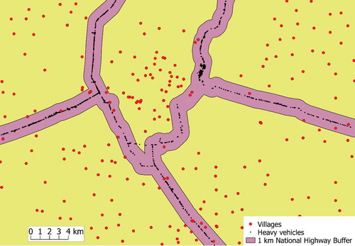
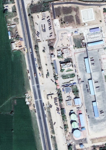
We used Google Earth satellite imagery to identify trucks and buses across the whole network of national highways (∼430 km) in the state. In QGIS, the satellite imagery was imported using “OpenLayers” plugin. Next, the GIS layer of national highways was overlaid on the imagery to guide the data collection. National highways are constructed and maintained by NHAI, a federally funded agency, and are intended for interstate long-distance connectivity. Therefore, long-distance heavy vehicles are more likely to move on those. A new point layer was created by geocoding every heavy vehicle identified (see Figure 2). This work was carried out by one researcher (RG). The buses and trucks are easily identified given that their size is much larger than other motorized modes in India such as cars, vans, and auto rickshaws. We did not attempt to differentiate between buses and trucks as this could have resulted in misclassification. The year of the imagery varied from 2015 to 2018, which is indicated in the lower right corner of the image. Therefore, observations of traffic across the state belonged to 1 of these 4 years. Data collection was restricted to national highways and the abutting land-use (see Figure 3).

Figure 3. A Google Earth screenshot of the satellite imagery showing trucks on the highway and nearby land-use (source: Google Earth snapshot).

Since satellite image is a snapshot and captures traffic across space, therefore, a greater number of vehicles will be detected in a district simply because that district covers a greater length of national highways. Therefore, a better measure of traffic is traffic density, defined as the number of vehicles per unit length of roadway, which is a traditional measure in traffic flow theory. Accordingly, we calculated the number of vehicles per unit length of national highway in the district. We refer to this variable as heavy vehicle density. To calculate this density, we assigned all the geocoded points to their respective districts. Next, for each district, we calculated heavy vehicle density by dividing the total number of geocoded heavy vehicles in a district by the total length of national highways in that district.

2.1. Regression model

We modelled fatalities as Poisson-lognormal mixture using Bayesian hierarchical modelling. The regression modelling was done using R-INLA (Rue et al., 2009), an R package, which employs integrated nested Laplace approximations to estimate the posterior distributions. The package has been used for injury modelling by DiMaggio (2015) for census tracts in New York city, Goel et al. (2018) for wards in Delhi, and Goel (2018) for states in India. The hierarchical model is described as follows: (1) $$y_n=\mathit{Poisson}\left(f_n\right)$$(1) (2) $$\log \left(f_n\right)=\log \left(p_n\right)+{\mathrm{\beta }}_0+\mathrm{\beta }{\mathrm{X}}_n+{\mathrm{\mu }}_n+{\mathrm{\delta }}_n+{\mathrm{\phi }}_t+{\mathrm{\gamma }}_{tn}$$(2) (3) $${\mathrm{\delta }}_n\sim N(0,1/{\tau }_{\mathrm{\delta }})$$(3) (4) $${\log (\tau }_{\mathrm{\delta }})\mathrm{}\sim \log \mathrm{Gamma}(1,0.0005)$$(4) where, $y_n\mathrm{}$ are the observed annual fatality counts of all road users in district $n,$ $f_n$ are the expected count of fatalities, ${\mathrm{X}}_n$ represents a vector of explanatory variables, $p_n$ is the population as an offset, ${\mathrm{\beta }}_0$ is the intercept,$\mathrm{}\mathrm{\beta }$ is a vector of fixed effect parameters, ${\mathrm{\mu }}_n$ is the uncorrelated heterogeneity or unstructured error,$\mathrm{}{\mathrm{\delta }}_n\mathrm{}$ is the spatially structured error, ${\mathrm{\phi }}_t$ is the structured temporal effect, and ${\mathrm{\gamma }}_{tn}$ is the spatio-temporal interaction effect. Here ${\mathrm{\delta }}_n\mathrm{}$ has the intrinsic conditional autoregressive (CAR) specification as proposed by Besag et al. (1991) and ${\mathrm{\phi }}_t$ is the first-order random walk-correlated time variable. Further details can be seen in DiMaggio (2015) and Goel et al. (2018).

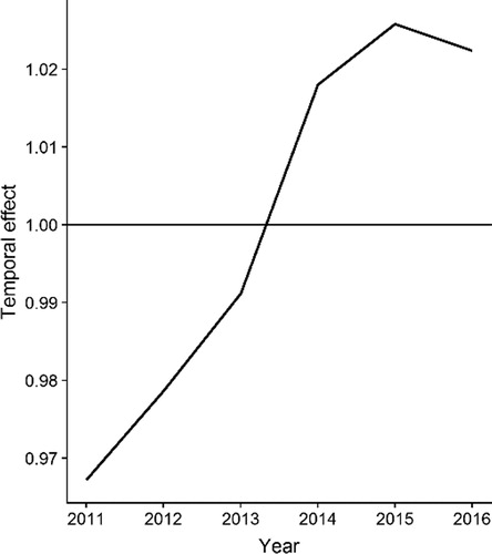
We first fitted a frailty model with no covariates and with only spatially structured error (${\mathrm{\mu }}_n),$ unstructured error (${\mathrm{\delta }}_n)$ and auto-correlated year effect (${\mathrm{\phi }}_t$). The temporal trend$({\mathrm{\phi }}_t$) term is shown in Figure 4, and shows that it has the least variation over the 3-year period from 2014 to 2016. These years are also closest to the satellite imagery (2015–2018) used for estimating heavy vehicle traffic. Therefore, for the regression analysis we included time series from 2014 to 2016 . We assume that the traffic movement does not vary greatly over the years, so that the mismatch between the time period of road fatality data and that of satellite imagery does not affect our analysis. All other variables were considered constant across this period. For sensitivity analysis, we used road deaths for the 6-year period (2011–2016) in the regression analysis.

Figure 4. Temporal effect of fatality rates.

The covariates at the district level used in the regression model are presented in Table 1 and have been described in Section 2. These include number of workers travelling to work by different modes of transport denoted as walk commuters, cycle commuters, m2w commuters, car commuters, ipt commuters, bus commuters, and train commuters. The other covariates include rural population and urban population which denote population living within 1 km of the national highways. Finally, heavy vehicle density denotes the heavy traffic volume. We fitted two sets of regression models, each with two models. In the first set, the two models include the model with only commuting-related variables (Model 1) and the second model (Model 2) with commuting-related variables and also controlling for rural and urban population. In the second set, the same two models were developed but the four variables walk commuters, bus commuters, train commuters, and ipt commuters were replaced by a new variable which combined walk with the three public transport modes (ipt, bus, and train) and is referred to as walk + PT commuters. This variable represents all the walking-related modes given that in Indian context each public transport trip is likely to include at least two walking trips in the form of access and egress. The two models in the second set with and without controlling for rural population and urban population are referred to as Models 3 and 4.

3. Results

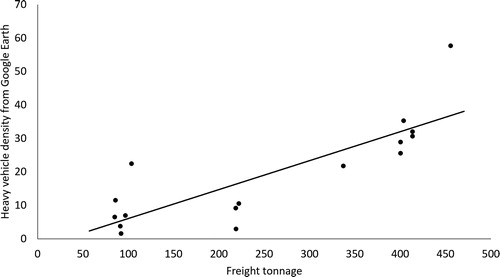
Using the observations from satellite images, we geolocated a total of 43,884 heavy vehicle. Heavy vehicle density on national highways vary from 43 to 1928 vehicles per km. To validate the estimate of heavy vehicle traffic, we used the freight tonnage reported for different national-highway sections as a part of nation-wide study conducted in 2007–2008 (RITES, 2014). For the corresponding road sections reported in the study, we estimated the heavy vehicle density as described above. We found that the two variables (freight tonnage and heavy vehicle density) are strong associated with a Pearson correlation of 0.84 (p < 0.001) (Figure 5). Although it should be noted that the tonnage data and Google Earth estimates of volume are separated in time by 7–8 years. Further, we estimated heavy vehicle traffic including both buses as well as trucks, while the comparison with the reported data is only for freight.

Figure 5. Observed freight tonnage and GE estimates of heavy vehicle density for selected road sections.

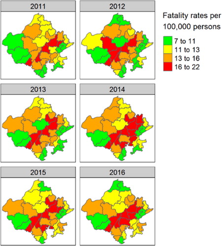
Figure 6 presents the relationship between heavy vehicle density and fatality rates. For this plot, fatality rates are the average over 2014–2016 period. The Pearson correlation between the two variables is 0.63 (p < 0.001) and excluding the three highest values of heavy vehicle density, the correlation value is 0.45 (p < 0.01). Figure 7 presents year-specific plot of fatality rates at the district level. There are some districts that have consistently high-risk levels across the years. The districts highlighted in red lie along the major corridor that connects Delhi with the Mumbai port.

Figure 6. A scatterplot showing district-level death rates and heavy vehicle density on national highways.

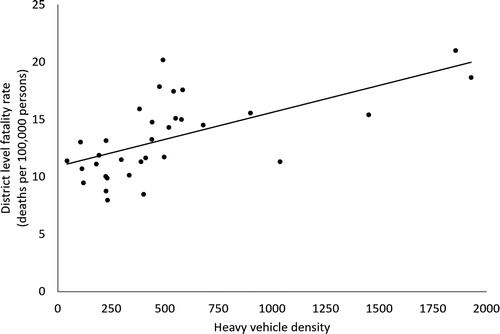
Figure 7. Year-specific fatality rates of districts of Rajasthan state.

The results of the four regression models are presented in Table 2 with mean and standard deviation (SD) of the posterior distributions of the coefficients. To compare the performance of Bayesian models, Deviance information criterion (DIC) is estimated which is a Bayesian version of Akaike information criterion (AIC). Similar to AIC, lower value of DIC implies higher predictive accuracy.

Table 2. Regression results.

	Mean (SD)
Variable	Model 4	Model 3	Model 2	Model 1
Intercept	−9.120(1.464)	−8.525(1.311)	−12.433(1.860)	−9.167(1.427)
log(heavy vehicle density)	0.149(0.078)	0.170(0.072)	0.130(0.076)	0.177(0.077)
log(car commuters)	0.238(0.131)	0.218(0.127)	0.323(0.125)	0.243(0.130)
log(m2w commuters)	−0.076(0.170)	−0.004(0.151)	−0.492(0.231)	−0.100(0.182)
log(cycle commuters)	−0.005(0.115)	−0.062(0.098)	0.331(0.174)	0.019(0.130)
log(walk commuters)			0.087(0.195)	−0.085(0.197)
log(train commuters)			−0.195(0.079)	−0.077(0.068)
log(bus commuters)			−0.055(0.103)	−0.042(0.111)
log(ipt commuters)			0.014(0.078)	−0.002(0.085)
log(walk + PT commuters)	−0.238(0.186)	−0.222(0.182)
log(rural population)	0.094(0.096)		0.297(0.120)
log(urban population)	−0.018(0.029)		−0.058(0.031)
DIC	906.62	906.51	906.68	906.57

The most consistent finding across all the models is that heavy vehicle density and car commuters have positive associations with fatality risk, and combined walk and PT usage have a negative association. Further, the magnitudes of the effects of heavy vehicle density and car commuters are the highest, consistently across the models. Rural population living in proximity to highways has a positive association, while urban population has a negative association, though rural population has a much larger effect size than urban population. All these variables except urban population in proximity to highways also have strong statistical significance.

The two variables, namely cycle commuters and walk commuters, show changing signs across the models and weaker statistical significance compared with other variables. Cycle commuters has a positive sign in Models 1 and 2 and negative sign in Models 3 and 4. Walk commuters has a negative sign in Model 1 but a positive sign in Model 2. The variable m2w commuters (motorized two-wheelers) also show large variation across the models. This variable has a high magnitude in Model 2 but its magnitude reduces to almost zero in Model 3.

Comparison of Models 1 and 3 with their more controlled counterparts (Models 2 and 4, respectively, including rural and urban population in proximity to highways) shows that the effect of heavy vehicles is weakened, both in magnitude, from 0.18 (Model 1) to 0.13 (Model 2) and from 0.17 (Model 3) to 0.15 (Model 4), as well as in statistical significance. In contrast, the effect of car commuters is strengthened in both respects (magnitude: 0.24–0.32 and 0.22–0.24). In other words, the effects of trucks and cars are modified, though the direction of association remains the same, when the population directly exposed to highway traffic is accounted for in the models.

To test the sensitivity of results to the inclusion of variable of heavy vehicle volume, we compared the results of Models 1 and 3 with their respective models without this variable (not shown in Table 2). We found that in Model 1, without the inclusion of heavy vehicle variable, the coefficient of cycle commuters increases by more than five times in magnitude (0.02–0.10), while that of bus commuters changes from negative to positive (−0.04 to 0.02). In Model 3, the effect of m2w commuters also increases significantly in magnitude. Therefore, it seems that, in the absence of heavy vehicle variable, its effect is absorbed by other modes. We also present the results of the four models with data for the 6-year period (Table A1 in appendix). The results show only slight reduction in effect size of most variables while the direction of association remains the same for all. Therefore, the conclusions of the regression models are independent of the years for which road deaths data has been used.

4. Discussion

4.1. Statement of principal findings

We estimated heavy vehicle (buses and truck) volume on national highways using Google Earth satellite images. We found that the estimated volume correlate reasonably well with the traffic counts reported in a government study, with a Pearson correlation of 0.84 (p < 0.001) We used Google Maps API for large-scale mapping of villages and cities to estimate population living in proximity to the highways. We further fitted a spatiotemporal regression model using Bayesian modelling framework with number of road deaths at the district level as the outcome variable. The model results indicate that heavy vehicle density has a positive association with road deaths. Rural population living in proximity to national highways has a positive association while urban population have a negative association. Among the passenger modes of travel, car is positive associated while combined walking and public transport usage has a negative association with road deaths. We also found that not accounting for heavy vehicle volume results in omitted variable bias in the model results. In our models, this was reflected in the effects of other modes of travel, which were biased upwards.

4.2. Strengths and weaknesses of the study

Traffic volume is an important factor contributing to traffic injuries (Aldred et al., 2018; Elvik et al., 2009) and, therefore, essential for epidemiological investigation of traffic injuries. In countries such as India and other LMICs, there are no mechanisms to ensure systematic collection of traffic counts in the cities or highways. In accident prediction models, lack of such variables can result in omitted variable bias (Elvik, 2011; Goel, 2018; Mitra & Washington, 2012). This study presents a novel method to estimate traffic volume of heavy vehicles. This is the first study to use satellite-imagery based vehicle count at a large scale for epidemiological research. We also used Google API for large-scale mapping of rural settlements. The methods presented here are easily replicable in virtually every setting in the world as both Google Earth and Google Maps API have a global coverage, and the use of former is free of cost while the cost of using the latter can be minimized with a limited daily use of the API.

While this study presents an area-level analysis, these methods can potentially be replicated for micro-level studies. Future studies should investigate the potential of satellite imagery to estimate traffic volume at the street level and investigate if these methods work at smaller scale. While the identification of vehicles in this study was limited to heavy vehicles, this method can be extended to include other motor vehicles of smaller size such as cars, vans, and three-wheeled auto rickshaws. However, with the given resolution of Google Earth for India, it is not possible to differentiate between these vehicles. Within Google Earth, there are variations in the resolution of the imagery across the countries. In India, the images are likely 15 m resolution. In North America and western Europe, Google Earth images are often obtained through aerial data collection which includes photography using an aeroplane and such images can have resolution up to 0.15 m. High-resolution images of 1 m or lower can also be obtained through other satellites such as WorldView-2 or Quickbird, however, these are not available for free.

There are certain limitations in our work. In Google Earth, the year corresponding to the imagery was found to vary across the state, which is likely to bring spatial bias in the estimates of heavy vehicles. Further, heavy vehicle identification was restricted to only national highways. For two districts with high volume of heavy vehicle, we found that the volume of state highways is only a minor fraction of the volume of national highways, therefore, this is less likely to result in any bias. It is an ecological study and, therefore, has the limitation arising from modifiable area unit problem. A district comprises of cities as well as villages, and highways as well as urban streets. At an aggregate level, these differences are not accounted for. Further, the traffic volume estimates from Google Earth needs to be validated for other settings and road types.

4.3. Meaning of the study: possible mechanisms and implications for policymakers

The study results highlight the implications of freight policies on road traffic injuries. India has much higher share of its freight movement through road compared to other large countries such as the USA and China (McKinsey, 2009). In India, policy discussions of mode shift of freight in favour of railways often occur in the context of transport efficiency, energy use, greenhouse gas emissions or air quality (Dhar & Shukla, 2015). However, evidence from this study as well as from previous research (Goel, 2018; Mohan et al., 2016; Naqvi & Tiwari, 2017) highlights that on-road freight movement has significant implications for traffic injuries. Therefore, policy formulation around freight movement should account for traffic injuries as one of the externalities.

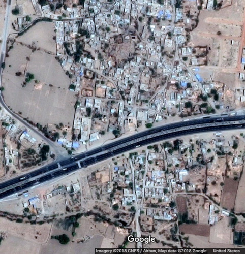
A positive association between rural population living in proximity to national highways and death rates has important implications. Highways in India often pass through the villages and towns or run in their vicinity (e.g. Figure 8). Since people in Indian villages predominantly travel by walking, cycling or use motorized two-wheelers (Census-India, 2017), their exposure to high-speed heavy traffic on highways results in serious injuries or deaths. As a result, the three road users contribute up to 60% of all road deaths victims on Indian highways (Naqvi & Tiwari, 2017). It is a remarkably high proportion given that highways are often thought of as being used exclusively by cars and trucks. Given the rapid growth of highway network in India (NHDP, 2019), it is important that future development of highways minimize proximity to the inhabited rural areas. In contrast to the rural population, the association of urban population in proximity to highways has a negative association with the fatality rates. It is possible that highways close to urban areas tend to be congested in the vicinity of urban areas, and as a result, tend to have lower rates of fatalities. We should note that the effect size of urban population in proximity to highways is much smaller than rural population.

Figure 8. A six-lane national highway passing through a village (Source: Google Earth snapshot).

4.4. Unanswered questions and future research

Google Earth is a freely available data source and covers the entire world. While the identification of vehicles in this study was limited to heavy vehicles, this method can be extended to include other motor vehicles such as three-wheeled auto rickshaws and cars. Further, distinction can also be made between trucks and buses. The possibility to detect pedestrians, cyclists and motorcycles from overhead satellite images is unlikely.

Further, the potential application of these data are not limited to traffic safety epidemiology. These new data sources can be further applied to estimate travel patterns at the city level. While our study used manual annotation, this work can be scaled up by using machine learning based image recognition (Cao et al., 2016). The methods presented here can be replicated at the city level as well as scaled up for the whole country.

Acknowledgements

Contributions from R. G. and J. W. were undertaken under the auspices of the Centre for Diet and Activity Research (CEDAR), a UKCRC Public Health Research Centre of Excellence funded by the British Heart Foundation, Cancer Research UK, Economic and Social Research Council, Medical Research Council, the National Institute for Health Research (NIHR) and the Wellcome Trust (MR/K023187/1). R. G., J. J. M., N. G., and J. W. were supported by TIGTHAT, an MRC Global Challenges Project.

Disclosure statement

No potential conflict of interest was reported by the authors.

Appendix

Table A1. Regression model using fatality data for the 6-year period from 2011 to 2016.

	Mean (SD)
Intercept	Model 4	Model 3	Model 2	Model 1
log(heavy vehicle density)	−9.610 (1.381)	−8.987 (1.243)	12.527 (1.745)	−9.363 (1.350)
log(car commuters)	0.127 (0.074)	0.148 (0.068)	0.100 (0.071)	0.145 (0.073)
log(m2w commuters)	0.213 (0.123)	0.192 (0.120)	0.292 (0.117)	0.213 (0.123)
log(cycle commuters)	−0.061 (0.161)	0.014 (0.143)	−0.473 (0.217)	−0.092 (0.172)
log(walk commuters)	0.024 (0.109)	−0.036 (0.093)	0.351 (0.163)	0.048 (0.123)
log(train commuters)			0.054 (0.183)	−0.112 (0.187)
log(bus commuters)			−0.186 (0.074)	−0.072 (0.064)
log(ipt commuters)			−0.039 (0.097)	−0.026 (0.105)
log(walk + PT commuters)			0.053 (0.074)	0.037 (0.080)
log(rural population)	−0.211 (0.176)	−0.194 (0.173)
log(urban population)	0.099 (0.091)		0.289 (0.113)
DIC	−0.02 (0.028)		−0.057 (0.029)
Intercept	1788.09	1788.05	1788.19	1788.1

References

- Aldred, R., Goodman, A., Gulliver, J., & Woodcock, J. (2018). Cycling injury risk in London: A case-control study exploring the impact of cycle volumes, motor vehicle volumes, and road characteristics including speed limits. Accident; Analysis and Prevention, 117, 75–84. https://doi.org/10.1016/j.aap.2018.03.003
- Besag, J., York, J., & Molli, A. (1991). Bayesian image restoration, with two applications in spatial statistics. Annals of the Institute of Statistical Mathematics, 43(1), 1–20. https://doi.org/10.1007/BF00116466
- Cao, L., Wang, C., & Li, J. (2016). Vehicle detection from highway satellite images via transfer learning. Information Sciences, 366, 177–187. https://doi.org/10.1016/j.ins.2016.01.004
- Census-India. (2017). B-28 'Other Workers' by distance from residence to place of work and mode of travel to place of work – 2011. http://www.censusindia.gov.in/2011census/B-series/B_28.html
- Chang, A. Y., Parrales, M. E., Jimenez, J., Sobieszczyk, M. E., Hammer, S. M., Copenhaver, D. J., & Kulkarni, R. P. (2009). Combining Google Earth and GIS mapping technologies in a dengue surveillance system for developing countries. International Journal of Health Geographics, 8(1), 49. https://doi.org/10.1186/1476-072X-8-49
- Datta, S. (2012). The impact of improved highways on Indian firms. Journal of Development Economics, 99(1), 46–57. https://doi.org/10.1016/j.jdeveco.2011.08.005
- Desapriya, E., Subzwari, S., Sasges, D., Basic, A., Alidina, A., Turcotte, K., & Pike, I. (2010). Do light truck vehicles (LTV) impose greater risk of pedestrian injury than passenger cars? A meta-analysis and systematic review. Traffic Injury Prevention, 11(1), 48–56. https://doi.org/10.1080/15389580903390623
- Dhar, S., & Shukla, P. R. (2015). Low carbon scenarios for transport in India: Co-benefits analysis. Energy Policy, 81, 186–198. https://doi.org/10.1016/j.enpol.2014.11.026
- Dimaggio, C. (2015). Small-area spatiotemporal analysis of pedestrian and bicyclist injuries in New York City. Epidemiology (Cambridge, MA), 26(2), 247–254. https://doi.org/10.1097/EDE.0000000000000222
- Eikvil, L., Aurdal, L., & Koren, H. (2009). Classification-based vehicle detection in high-resolution satellite images. ISPRS Journal of Photogrammetry and Remote Sensing, 64(1), 65–72. https://doi.org/10.1016/j.isprsjprs.2008.09.005
- Elvik, R. (2011). Assessing causality in multivariate accident models. Accident; Analysis and Prevention, 43(1), 253–264. https://doi.org/10.1016/j.aap.2010.08.018
- Elvik, R., Vaa, T., Hoye, A. and Sorensen, M. (Eds.). (2009). The handbook of road safety measures. Emerald Group Publishing.
- Goel, R. (2018). Modelling of road traffic fatalities in India. Accident; Analysis and Prevention, 112, 105–115. https://doi.org/10.1016/j.aap.2017.12.019
- Goel, R., Jain, P., & Tiwari, G. (2018). Correlates of fatality risk of vulnerable road users in Delhi. Accident; Analysis and Prevention, 111, 86–93. https://doi.org/10.1016/j.aap.2017.11.023
- Goel, R., Mohan, D., Guttikunda, S. K., & Tiwari, G. (2016). Assessment of motor vehicle use characteristics in three Indian cities. Transportation Research Part D: transport and Environment, 44, 254–265. https://doi.org/10.1016/j.trd.2015.05.006
- Hamilton, S. E., Talbot, J., & Flint, C. (2018). The use of open source GIS algorithms, big geographic data, and cluster computing techniques to compile a geospatial database that can be used to evaluate upstream bathing and sanitation behaviours on downstream health outcomes in Indonesia, 2000–2008. International Journal of Health Geographics, 17(1), 1–11.
- Kumar, M., Singh, S., Ghate, A. T., Pal, S., & Wilson, S. A. (2016). Informal public transport modes in India: A case study of five city regions. IATSS Research, 39(2), 102–109. https://doi.org/10.1016/j.iatssr.2016.01.001
- Larsen, S. Ø., Salberg, A.-B., & Eikvil, L. (2013). Automatic system for operational traffic monitoring using very-high-resolution satellite imagery. International Journal of Remote Sensing, 34(13), 4850–4870. https://doi.org/10.1080/01431161.2013.782708
- Malik, L., &Tiwari, G. (2017). Assessment of interstate freight vehicle characteristics and impact of future emission and fuel economy standards on their emissions in India. Energy Policy, 108, 121–133.
- McKinsey (2009). Building India: Transforming the nation’s logistics. India: McKinsey & Company. https://www.mckinsey.com/industries/travel-transport-and-logistics/our-insights/transforming-indias-logistics-infrastructure
- Mitra, S., & Washington, S. (2012). On the significance of omitted variables in intersection crash modeling. Accident; Analysis and Prevention, 49, 439–448. https://doi.org/10.1016/j.aap.2012.03.014
- Mohan, D., Tiwari, G., & Mukherjee, S. (2016). Urban traffic safety assessment: a case study of six Indian cities. IATSS Research, 39(2), 95–101. https://doi.org/10.1016/j.iatssr.2016.02.001
- MoRTH. (2017). Road accidents in India – 2016. India: Ministry of Road Transport and Highways Transport Research Wing.
- Naqvi, H. M., & Tiwari, G. (2017). Factors contributing to motorcycle fatal crashes on national highways in India. Transportation Research Procedia, 25, 2084–2097. https://doi.org/10.1016/j.trpro.2017.05.402
- NCRB. (2015). ADSI Reports of Previous Years. National Crime Records Bureau. http://ncrb.gov.in/StatPublications/ADSI/PrevPublications.htm
- NHAI. (2017). State-wise length of National Highways (NH) in India as on 30.06.2017. http://www.nhai.org/writereaddata/Portal/Images/pdf/StateWiseLengthNHsIndia.pdf
- NHDP. (2019). National Highways Development Project. Retrieved on March 7, 2019, from http://www.nhai.org/about-nhdp.htm
- Paulozzi, L. J. (2005). United States pedestrian fatality rates by vehicle type. Injury Prevention : Journal of the International Society for Child and Adolescent Injury Prevention, 11(4), 232–236. https://doi.org/10.1136/ip.2005.008284
- Rajasthan Tourism Department. (2014). Tourism Department Annual Progress Report 2013–14. http://www.tourism.rajasthan.gov.in/content/dam/rajasthan-tourism/english/others/tourism-department-annual-progress-report-2013-14.pdf
- RITES. (2013). Total transport system study on traffic flows and modal costs (highways, railways, airways and coastal shipping). In A study report for the Planning Commission. India: The Government of India.
- Rue, H., Martino, S., Lindgren, F., Simpson, D., Riebler, A., & Krainski, E. (2009). INLA: functions which allow to perform a full Bayesian analysis of structured additive models using Integrated Nested Laplace Approximation. R package version 0.0.
- Schepers, J. P., & Heinen, E. (2013). How does a modal shift from short car trips to cycling affect road safety? Accident; Analysis and Prevention, 50, 1118–1127. https://doi.org/10.1016/j.aap.2012.09.004
- Tang, T., Zhou, S., Deng, Z., Zou, H., & Lei, L. (2017). Vehicle detection in aerial images based on region convolutional neural networks and hard negative example mining. Sensors, 17(2), 336. https://doi.org/10.3390/s17020336
- Tiwari, P., & Gulati, M. (2013). An analysis of trends in passenger and freight transport energy consumption in India. Research in Transportation Economics, 38(1), 84–90. https://doi.org/10.1016/j.retrec.2012.05.003