More than surface temperature: mitigating thermal exposure in hyper-local land system

ABSTRACT

Regional land surface temperature (LST) maps derived from remote sensing data are most available to cities to assess and respond to heat. Yet, LST only captures one dimension of urban climate. This study investigates the extent to which remote sensing derived estimates of LST are a proxy for multiple climate variables at hyper-local scales (<10s of meters). We compare remotely sensed estimates of LST (RS-LST) to field and simulated LST, MRT, and air temperature (AT), in a neighborhood in Tucson, Arizona, USA. We find that LST, MRT, and ST follow different diurnal trends masked by RS-LST. We also find that three-dimensional urban design is a better predictor of MRT than two-dimensional land cover and albedo – a known determinant of RS-LST. Shade is a better predictor of both simulated LST and MRT than RS-LST. We conclude that RS-LST is not adequate for guiding heat mitigation at hyper-local scales in cities.

KEYWORDS:

• Climate adaptation
• thermal comfort
• extreme heat
• urban planning
• New Urbanism
• urbanization
• remote sensing
• land use planning

Introduction

Land cover plays a large role in determining the thermal conditions in cities, which is an increasingly urgent concern in cities around the world that must contend with increasingly extreme and inequitable heat impacts. Regional climate science has unequivocally established the connection between urban land features such as buildings, roads, and parking lots and hotter land surface temperature in cities than proximate undeveloped, vegetated land: the urban heat island phenomenon (UHI)(Bowler et al., 2010; Deilami et al., 2018; Oke, 1982; Voogt & Oke, 2003). These studies direct attention toward the role of density of vegetation and albedo in regulating land surface temperature (LST) by controlling evaporation and the amount of solar radiation reflected off a surface. Building on this insight, land systems scholars have found that, in addition to the extent of high albedo surface materials and trees, the spatial arrangement of urban land features also explains heterogeneity in LST across neighborhoods within cities (Connors et al., 2013; X. X. Li et al., 2016; Mohajerani et al., 2017). LST, albedo, and vegetative density (e.g. Normalized Difference Vegetation Index, NDVI and Soil Adjusted Vegetation Index, SAVI) are relatively easily derived from remote sensing data products that are publicly available over large spatial extents, at fine resolutions, and many are free. As such, LST maps are widely available for use by cities to guide decision-making on heat mitigation and adaptation (L. Keith et al., 2019). Yet, cities have a variety of cooling goals, many of which are contingent on factors beyond LST, albedo, and vegetative density. For instance, mean radiant temperature (MRT) is a composite indicator that more closely characterizes the thermal burden of heat on the human body than LST. The strongest predictor of MRT is shade, which controls the amount of exposure to incoming solar radiation a person is exposed to as opposed to surface albedo (Middel et al., 2016). In fact, high albedo, LST mitigating surfaces can re-radiate heat, causing increased thermal burden for pedestrians during midday hours (Erell et al., 2014; Middel et al., 2020). High resolution, spatial data on MRT is not, however, currently available at a city scale for use by decision-makers. There is a potential mismatch, therefore, between the type of information provided through conventional remote sensing-based land systems data outputs and the type of information that cities need to make effective decisions (Ladd Keith et al., 2021; Mackey et al., 2017).

This study examines the appropriateness of remote sensing-based temperature data in guiding municipal heat planning beyond UHI mitigation through the overarching question: To what extent is LST data derived from remote sensing analysis a proxy for a larger range of climate conditions captured through field and simulated data? To address this question, we compare relationships between the built environment and multiple temperature variables: remote sensing derived LST and field and simulated LST, air temperature (AT), and MRT. Specifically, we ask the following empirical questions: (1) How do temperature variables vary diurnally in comparison to one another? (2) Does LST predict temperature variables? (3) Which urban land features explain variation in temperature variables? Data are drawn from remote and in situ observations and microclimate simulations of Civano, a planned community in Tucson, Arizona, USA, that is known to have reduced LST through clustering of high albedo surface materials and vegetation, compared to similar, adjacent sites (Turner & Galletti, 2015). The findings are discussed with respect to implications for municipal heat planning specifically, and the use of remote sensing data in climate adaptation planning more broadly. We discuss synergies and tradeoffs across temperature variables in the context of two urban planning goals: urban heat island mitigation, which highlights the importance of surface albedo and vegetative density, and improving thermal comfort, which is more nuanced and largely influenced by incoming solar radiation and radiative heat.

Disambiguating the role of urban land in moderating heat in cities

Heat has become a central concern to cities around the world. While heat has always been a concern in major hot climate cities such as Dubai, Phoenix, and New Delhi, climate change has forced cities everywhere to confront the challenges of a hotter future. In 2021, for example, extreme heat in the temperate Pacific northwest United States and Canada broke temperature records observed in hotter regions: Lytton, Canada, north of 50°N, broke the heat record of Las Vegas, United States – a city with a hot desert climate at 36°N (Di Liberto, 2021, June). Most models predict that cities will experience increased average high and low temperatures, more frequent and severe extreme heat events, and a longer heatwave season (Jones et al., 2015; Meehl & Tebaldi, 2004). In this context, cities have become increasingly aware of the role that conventional urban land development plays in exacerbating extreme heat conditions, as well as the central role alternative approaches will need to play in mitigating and adapting to a hotter future. Moreover, heat exposure and health impacts are inequitable, disproportionately affecting the low income and communities of color (Chambers, 2020; Hoffman et al., 2020; Sheridan et al., 2021). Yet, not all extreme heat is urban – and not all urban heat is extreme – therefore, it is essential to disambiguate the ways that urbanization directly contributes to hotter or cooler conditions in cities.

Broadly, urban land controls thermal conditions in cities through the regional UHI, local climate zones, and hyper-local climate regulation. Regionally, urban land contributes to the UHI phenomenon through which low albedo built materials such as buildings, roads, and parking lots absorb incoming solar radiation and slowly reradiate it as heat, leading to elevated afternoon and evening temperatures compared to undeveloped areas (Arnfield, 2003). The most efficient way to reduce UHI is through high albedo, reflective surfaces such as white roofs that reduce LST or through increased vegetative cover, which cools ground surfaces through shading and air temperature through evapotranspiration. Within cities, there is significant heterogeneity in LST, and the spatial arrangement of land features is known to augment thermal conditions (Buyantuyev et al., 2010; Connors et al., 2013; X. X. Li et al., 2016; Liao et al., 2021). At the neighborhood scale (100s–1000s square meters), Local Climate Zones (LCZs) highlight the importance of the three-dimensional environment in addition to surface materials (Stewart & Oke, 2012). Recent work has found, for example, that LCZs with more compact buildings tend to have higher LST and near surface AT (Kotharkar & Bagade, 2018; Thomas et al., 2014; Yang et al., 2020). LCZ studies find that mechanisms such as the amount of shade also influence the neighborhood heat distribution in addition to surface materials (Middel et al., 2014). Urban climate is highly sensitive to hyper-local (10s square meters or less) variation in the built environment; ST and MRT are especially sensitive to the built environment and can vary between points just a few feet apart due to micro-variation in surface material and sun exposure (Salata et al., 2016). AT, on the other hand, is relatively ubiquitous at hyper-local scales and not as sensitive to urban design features as LST and MRT. Municipal planning for regions, neighborhoods, and sites, therefore, must consider different features of urban land and different types of temperature to achieve ‘cooling.’

Yet, UHI is the dominant framing for urban heat problems and regional LST–and sometimes regional AT–maps are the most prevalent tools at the disposal of cities, if they have any data at all (Keith et al., 2019; Meerow and Keith 2021). A major reason why LST maps are so prevalent is that spatial data are readily available and straightforward to process for entire regions. AT mapping requires modeling sophistication that some cities may not have access to, and MRT data requires field data collection and and model simulations using specialized software only capable of small spatial extents. The variety of ways that urban land influences thermal conditions in cities has, therefore, been collapsed to just a small subset of urban heat dynamics

Martilli et al. (2020) review a variety of reasons that UHI has conceptual shortcomings in guiding municipal heat planning. Fundamentally, it describes a very specific, regional phenomenon–and, perhaps, is better described as the regional urban heat island (RUHI)–based on a comparison between urban and proximate rural and undeveloped regions. The scale of the phenomenon is mismatched with the sub-city scale of many municipal heat problems (e.g. pedestrian thermal burden) or urban land interventions. Moreover, UHI describes differences between urban and non-urban regions and may fail to capture the severity of urban heat in arid environments, where the introduction of irrigated urban land may actually cause some urban areas to have lower surface temperatures than the desert (Aram et al., 2019; Daniel et al., 2018). Additionally, regional models of urban climate reveal that the relative efficacy of reflective surfaces versus vegetation depends on regional context, and increasing vegetation, for instance, tree planting, is not without environmental trade-offs (Georgescu et al., 2014; Roman et al., 2020). The surface UHI (SUHI)–also frequently just called the UHI–is usually characterized using LST, which captures the importance of surface reflectivity in regulating temperature, but it leaves out other important aspects of urban climate such as humidity, wind speed, and radiant heat.

Operationalizing the UHI using regional LST maps to guide land planning is also potentially problematic. LST is frequently derived from satellite images taken at one time of day. For instance, one of the most commonly used remote sensing sources, Landsat, provides images taken at 10:00am. Single time-stamp images are not capable of capturing diurnal variation. This is problematic because LST, AT, and MRT all change throughout the day. The UHI phenomenon in particular is most pronounced in the late afternoon and early evening hours, so UHI estimates derived from Landsat imagery likely underestimate the effect (Turner and Galletti, 2014). Surface materials also radiate incoming solar radiation at different times of day: high albedo surface radiate energy quickly and thus peak earlier in the day during peak sunlight, while low albedo surfaces radiate energy more slowly throughout the day and peak later after sunlight has peaked (Middel et al., 2020). That is why the UHI effect, which is driven in large part by concentrations of low albedo surface in built-up areas, is most pronounced in the late afternoon and evening. Robust analysis of LST incorporates multiple sensors across a period of days, months, or years (Yang et al., 2020). More recent and novel use of remote sensing data estimate MRT using LST and ancillary products (e.g. LiDAR). It is unlikely that such analyses are widely used by municipalities that report difficulty obtaining LST maps (Meerow & Keith 2021).

Regional LST maps are also typically generated at coarse resolutions, which introduces several measurement biases. Free and widely available maps like Aster (15 square meters), Landsat (30 square meters), and Ecostress (70 square meters) are too coarse to capture variation in LST temperature at hyper-local scales. Some private sector satellites provide temperature data at relevant scales (e.g. Quickbird, 1 square meter), but exist behind paywalls. LST is not a perfect proxy for actual ST. LST is an estimate of the Earth’s skin temperature based on atmosphere-level readings that is known to underestimate the actual surface temperature of built materials (J. K. Vanos et al., 2016). Additionally, remote sensing product can only measure surfaces ‘visible’ to the sensor. Therefore, an open question remains as to whether remote sensing data can reliably assess conditions such as shaded areas underneath trees and other objects (Cheung et al., 2021).

Potentially most problematic, however, is the fact that LST is just one of several types of temperature and most relevant for representing the regional UHI and not hyper-local urban heat challenges. Sub-neighborhood scale urban design and natural features control human thermal burden by determining exposure to incoming solar radiation and outgoing radiative heat from urban objects proximate to the body, in addition to controlling factors such as air flow. Yet, several studies have found that high albedo surfaces that reduce LST have little effect on or even decrease thermal comfort for people locally (Middel et al., 2020; Salata et al., 2015; Saneinejad et al., 2014). MRT, a composite indicator that factors in multiple factors that contribute to thermal burden, has been used as a closer proxy to the human experience of heat (Jennifer K. Vanos et al., 2010; Kruger et al., 2014). Providing shade is the most effective way to lower MRT, prevent bodies and surfaces from exposure to incoming solar radiation, reduce outdoor human thermal burden through urban land features in hot dry environments (Saneinejad et al., 2014). While differences exist in the effectiveness of different types of shade – depending on the transmissivity and material of the shade – all shade is substantially better at improving thermal comfort than none at all (Middel et al., 2021). AT also plays a large role in explaining thermal burden, but it is not as responsive to urban design as ST or MRT. This feedback effect would not likely be triggered at small spatial extents. In sum, LST does not capture the full suite of temperature variables that are important to consider in planning at hyper-local scales. An open question is the extent to which LST provides an adequate signal for those variables.

Temperature types may respond differently to urban land interventions. Using multiple measures of temperature makes trade-offs between UHI mitigation and human thermal burden visible: interventions like ‘cool streets’ effectively reduce surface temperatures, but also increase human heat burden during mid- to late afternoon hours (Middel et al., 2020). Hypothetical models that increase surface albedo over large areas like a region show that cool surfaces could reduce air temperatures and improve thermal comfort (Santamouris, 2013; Synnefa et al., 2007; may also reduce air temperature as well if the spatial extent is sufficiently large (Georgescu et al., 2014; Imran et al., 2018; Taha, 1997). Generally studies find that augmenting surface albedo will most directly influence LST (Taha, 1997). Shade interventions influence surface temperatures locally and the thermal burden experienced by humans (Middel et al., 2016). But, even tree shade can have unintended consequences, elevating AT in certain contexts (Cheung et al., 2021). Therefore, an important question for cities when designing cooling interventions is the extent to which LST versus solar exposure are relevant and which aspects of urban land moderate each.

Methods

Research questions and hypothesis

In order to elucidate the implications of using LST derived from remote sensing to guide hyper-local planning, we compare trends and relationships between remote, field observation, and model-derived data in order to answer to test the following hypotheses:

• 1. How do temperature variables vary diurnally in comparison to one another?

We hypothesize that LST and AT values will be highest in the afternoon and remain elevated during the evening due to heat retained in impervious surfaces. MRT will be highest midday and coolest after sunset due to the relationship with incoming solar radiation. It will also be the most variable based on the amount of shade from nearby objects.

• 2. Does LST predict temperature variables?

We hypothesize that remote sensing estimates of LST will be most predictive of simulated LST during the daytime, especially near the time when the remote sensing image was taken. Incoming solar radiation will be most predictive of simulated MRT because shade controls thermal comfort. Neither remote sensing estimates of LST or incoming solar radiation will predict AT.

• 3. Which urban land features explain variation in temperature variables?

We hypothesize that Land cover features, albedo, and SAVI will explain LST. Land design will explain MRT. AT will not relate to land features because the whole study area is one Local Climate Zone.

Study area

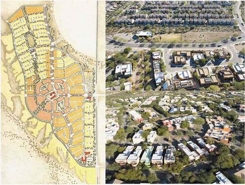
Civano (32°09ʹ19.5”N 110°46ʹ10.3”W), an environmentally sustainable planned development located 40 miles Southeast of Tucson, Arizona, USA in the Sonoran Desert. The climate is hot semi-arid (Koeppen, BSh) with an average annual rainfall of 299.7 mm. During the summer, temperatures above 38 degree Celsius are common (Meadow et al., 2019). Civano (Figure 1) is an early example of New Urbanist neighborhood design and, while heat mitigation was not a central goal, many of the design features intended to reduce energy and water use have heat mitigation co-benefits. For instance, the use of white roofs to reduce building energy consumption and the compact, networked building and road configuration, coupled with the use of washes and non-potable irrigation systems to create shaded pedestrian routes and encourage passive transportation, contribute to lower LST compared to adjacent neighborhoods (Turner & Galletti, 2015). The designers also focused on the use of building and street orientation to maximize passive cooling. Civano is an LCZ 6 C – typical of single family detached dwelling neighborhoods – characterized by open low rise buildings dominated by bush and scrub vegetation; however, the mixed-use imperative of New Urbanism created a more varied built environment than a typical suburban residential neighborhood. Civano is an ideal laboratory for comparative work because, developed in two phases–Civano I utilized the design features described here and Civano II (Sierra Morado) only used water and energy efficient buildings–and is adjacent to a conventional residential subdivision. While Civano I is known to contain land cover and configuration that produce an abundance of low LST census blocks, it also has a large variation in urban form (composition and two dimensional configuration of land cover), LST, albedo, and vegetation (a higher standard deviation than adjacent neighborhoods). New Urbanist design is intentionally heterogeneous and uses a wide variety of building types, set backs, road widths, alleys, and green spaces. Similar to a previous study on New Urbanist design and thermal comfort (Crewe et al., 2016), we take advantage of this internal heterogeneity to examine how hyper-local climate conditions might vary with urban design as well.

Figure 1. Civano Town Plan follows a conventional New Urbanist formula: the most compact housing (dark orange) is centrally located around a community center and the least compact housing is at the periphery of the development (yellow) (left, source: Moule & Polyzoides, Architects and Urbanists), larger ‘compound housing’ in Civano across the street from standard single family residential housing in Civano II (top right, source: James Nicholas Polyzoides), compact and centrally located ‘courtyard housing’ (bottom right, source: Stephanos Polyzoides).

Data collection

Dependent variable field observations in civano I: LST, MRT, AT

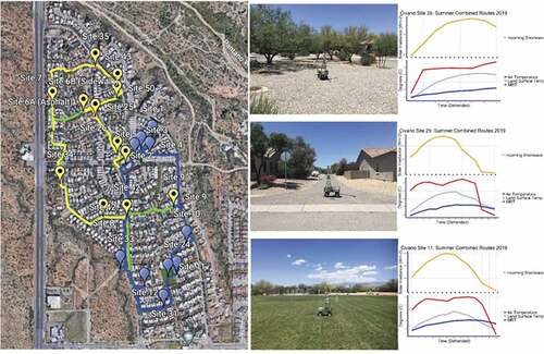
Field data measurements in Civano I were taken on a sunny, clear-sky day (25 May 2019) between 7:00 MST and 21:00 MST using two biometeorological MaRTy carts (Middel & Krayenhoff, 2019). Every 2 seconds, MaRTy records location (latitude/longitude), AT, relative humidity (RH), wind speed, and six-directional long- and shortwave radiant flux densities. A total of 23 sun-exposed or shaded locations with different surface properties were measured, though 5 of those locations were only measured until 14:00 MST due to a flat tire (Figure 2). A single measurement transect covered all locations approximately in 60 minutes, with 45 second stops to account for sensor lag (Häb et al., 2015). For details on data processing we refer to the method section of Middel and Krayenhoff (2019). Additionally, an overall comparison between sampled observed AT, ST, and MRT by surface cover type (asphalt, gravel, grass, concrete) and sun exposed versus shaded sites was conducted using the non-parametric difference in means test, the Kruskal-Wallis Test (Kruskal & Wallis, 1952).

Figure 2. Map of the 23 locations of field measurements, transect paths, and three example figures from sample sites that can be viewed using the interactive map online. To interact with the figure online and see figures with AT, ST, and MRT readings overlaid on the site LST map visit: https://studyingplace.space/civano/.

Dependent variables from microclimate modeling: simulated LST, MRT, AT

The processed MaRTy observations were used to validate ENVI-met model simulations, a microclimate modeling software, that extrapolated microclimate conditions to the entire study area. Urban design of the model domain was built from LiDAR point clouds, OpenStreetMap, and classified NAIP imagery. LiDAR data were converted to a canopy height map (CHM) using the lidR package in R (Roussel, 2021; Roussel et al., 2020). A digital terrain model was used to normalize the LiDAR data, values less than zero were removed, then the p2r algorithm in the lidR package was applied to create the CHM. Cells with values over 30 m were removed from the CHM. The CHM data was then filtered using NDVI data derived from NAIP imagery. CHM data where NDVI values were greater than 0.3 were retained. To identify individual crown polygons, a watershed analysis was performed on the filtered CHM data. Erroneous squares were removed by 1) simplifying the polygons to reduce the number of vertices, 2) removing polygons with five vertices or less, 3) buffering each polygon, 4) masking the NDVI-filtered CHM using the buffered crown polygons, and 5) rerunning the watershed analysis on the masked data. NAIP imagery and Google Earth were used to quality control the results Google Earth (7.3.2.5776), 2019). Points at the center of each polygon crown were identified, and the maximum height of each crown was spatially bound with the tree point data frame.

To model micro-scale climate conditions we used the modeling software, ENVI-met version 4.4.6 (Summer 2021 release), a non-hydrostatic Computational Fluid dynamics model that simulates surface-plant-air microscale interactions (Bruse, 2020; Bruse & Fleer, 1998; Middel et al., 2014). The digital representation of Civano was created through a three-step process. Buildings, surfaces, and vegetation were analyzed and coded in QGIS version 3.14 using 1 m resolution remote sensing imagery, LiDAR and OpenStreetMap (QGIS Development Team (Version 3.14), 2019 OpenStreetMap contributors, 2019). These data were assigned profile codes corresponding to respective thermal properties from the ENVI-met database system and imported into ENVI-met’s Monde software for digitization and the creation of area input files for model simulation. The abledo profiles were adjusted for the following surface profiles: Sandy Loam 0100SL (.15), Pavement 0100PP (.2), and Asphalt Road 0100ST (.1). Building walls and roof materials were set to the default setting – moderate insulation. Final edits and model geometry were processed in ENVI-met’s Spaces. Receptors were placed in corresponding areas where field data were collected in order to get high resolution modeled atmospheric conditions for comparison. Civano was subdivided into three 3D area input files with approximately 150 m overlap between each sub-area. The input files were set to a 1 m grid resolution and resulted in the following sizes: Area 1 (383x277x25), Area 2 (382x284x25), Area 3 (384x302x25). For meteorological forcing, we used meteorological conditions data from the Tuscon International Airport Station for 25 May 2019, the day field data were collected (Supplement 1). Soil conditions were set to xeric values gathered by Middel et al. (2014) (Supplement 2). Finally, each model was run for a 23 hour period, allowing for required spin-up time, starting at 0 hour, with a data output every 30 min.

To validate the ENVI-met microclimate model for each sub area of Civano, we placed receptors throughout the model that corresponded to locations where field measurements were taken using MaRTy. The receptors provided modeled temperature measurements that we could compare to observed temperature measurements recorded by MaRTy. To validate the accuracy of each subarea model we calculated model performance statistics as outlined by (Willmott, 1981) (Table 1). Finally, we conducted a non-parametric difference in means test, the Kruskal–Wallis Test, to compare simulated AT, ST, and MRT by surface cover type (asphalt, grass, concrete) and sun exposed versus shaded sites (Kruskal & Wallis, 1952).

Table 1. ENVI-met model performance

Area modeled	Performance metrics	Air temperature (◦C)	Mean radiant temperature (◦C)
Area 1	MBE	−0.53	5.65
	RMSE	1.03	9.63
	MAE	0.91	7.31
	d	0.99	0.90
Area 2	MBE	−0.57	0.6
	RMSE	1.12	9.72
	MAE	0.86	7.79
	D	0.98	0.88
Area 3	MBE	−0.09	6.63
	RMSE	0.89	7.33
	MAE	0.61	6.63
	D	0.99	0.9

Independent variables for regression models: remote sensing-derived data

Land cover and remote sensing derived estimates of LST, Albedo, and Soil Adjusted Vegetation Index (SAVI), were characterized using summertime 0.6 m NAIP imagery (15 June 2019) and 30 m Landsat 8 OLI images (27 May 2019), respectively. The Landsat Provisional Surface Temperature was derived from the Landsat Level-1 thermal infrared bands, ASTER Global Emissivity Database (GED), and NDVI data using a single-band approach (Cook, 2014). Under no clouds conditions, the average error in LST was −0.262°C based on North America measurements (Laraby & Schott, 2018). The 2014 raw LiDAR (Light Detection and Ranging) point cloud data was acquired from the United States Geological Survey (USGS). We derived the study area’s 1-m surface height model from the point cloud using ArcGIS 3D tools. The analysis includes Civano I and two adjacent communities that were part of a previous study (Turner & Galletti, 2015). This study compared Civano I, II, and the comparison, and found that albedo foremost, followed by SAVI, were positively correlated with LST. It found that clustering (configuration) of high albedo land cover positively correlated to lower LST.

Due to the sparse vegetation and abundant bare soil in the study areas, SAVI was chosen to assess local vegetation presence and greenness and was derived from the NAIP imagery. The index includes a transformation in the Normalized Difference Vegetation Index (NDVI) equation to minimize the influence of soil brightness from spectral vegetation indices involving red and near-infrared (NIR) wavelengths. Albedo was calculated using the Landsat infrared and visible bands with the following equation:

(((0.300 * Band 2) + (0.233 * Band 4) + (0.143 * Band 5) + (0.036 * Band 6) + (0.012 * Band 7) - 0.018)/0.724) * 0.0001

Random forest supervised classification was used in the Google Earth Engine environment to determine land cover types in our study areas (Google Earth Engine, 2019). The NAIP imagery was classified for eight land cover types including simple vegetation; trees; high, medium, and low albedo services; bare soil and gravel; water; and shadows. Ten neighborhood blocks were chosen to sample 10 points per land cover class for a total of 100 samples each, or 800 samples total. However, water was not present in every neighborhood block, so the 100 water sampling points were chosen from backyard and community swimming pools and fountains. We validated our results using accuracy assessments within the Google Earth Engine environment achieving an overall accuracy of 98.45%. The resulting land cover image was used for microclimate model analysis. Lastly, zonal statistics were calculated for Civano I, II, and the comparison community, to determine minimum, maximum and mean values for all derived datasets (refer to Figure 3(a)).

Figure 3. (a) Map of Civano I and II neighborhoods in relation to the comparison community; (b) Land Cover map of eight classified land cover types; (c) soil adjusted vegetation index indicating the largest prevalence of greenery in all neighborhoods;, (d) albedo with brightness summaries by neighborhood; (e) land surface temperature with temperature summaries by neighborhood; and (f) visualization of the LISA analysis showing the level of confidence for the locations of the coolest and hottest spots across all study areas.

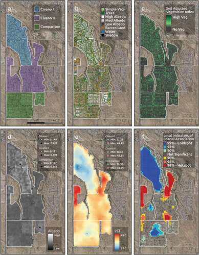
To account for local spatial autocorrelation (LISA) in the LST data set, the Hotspot Analysis QGIS plugin was used to identify spatial hot and cold spots in the data (Oxoli & Prestifilippo, 2017). The Hotspot Analysis computes Z-scores and p-values of the Gi* local statistic (Getis & Ord, 1992) for each geometry of a GIS file input (Oxoli & Prestifilippo, 2017). The resulting Gi* local statistic indicates clusters of high values (hot spot) and low values (cold spot).

Regression models to examine predictive power

To examine the predictive power of remote sensing based LST, shortwave radiation, and land cover variables on the simulated LST, MRT, and AT, we designed a series of linear regression models. Models 1 to 6 were univariate linear regression to test the predictive power of RS-LST and simulated shortwave radiation. Models 7 to 9 were multiple linear regression to examine the predictability of land cover variables, Albedo, and SAVI. We used the stepwise method to build the multiple linear regression models, in which the candidate predictors entered or removed from the model in a stepwise manner. To avoid multicollinearity, we also kept the VIF values low and removed those variables that show sign change during the stepwise process. The input predictors of model 7 to 9 were listed on the right side of the function. The final predictors that entered into the regression models are shown in Table 2, Table 3.

Table 2. Univariate linear regression results between Landsat 8 LST (RS-LST) and the simulated LST, MRT and AT at hour i and simulated shortwave radiation and simulated LST, MRT and AT at hour i at 30 m resolution. For RS-LST, all models are significant at 0.001 level (2-tailed) except for AT_15. For simulated shortwave radiation, all models are significant at 0.001 level (2-tailed) except for AT_08 and AT_15

RS-LST			Shortwave radiation
Simulated temperatures	R	R^2	Simulated temperatures	R	R^2
LST_08	−0.49	0.24	LST_08	0.05	0.003
LST_10	0.4	0.16	LST_10	0.69	0.47
LST_12	0.53	0.28	LST_12	0.76	0.58
LST_15	0.39	0.16	LST_15	0.48	0.23
LST_20	−0.72	0.52	LST_20	na	na
MRT_08	0.65	0.42	MRT_08	0.99	0.98
MRT_10	0.63	0.4	MRT_10	0.98	0.96
MRT_12	0.63	0.39	MRT_12	0.85	0.73
MRT_15	0.64	0.41	MRT_15	0.98	0.97
MRT_20	−0.67	0.45	MRT_20	na	na
AT_08	−0.1	0.01	AT_08	0.28	0.08
AT_10	0.17	0.03	AT_10	0.16	0.03
AT_12	0.25	0.06	AT_12	0.16	0.03
AT_15	0	0	AT_15	0.07	0.01
AT_20	−0.64	0.41	AT_20	na	na

Table 3. Multiple linear regression results between land cover variables and the simulated LST and MRT at hour i. **Correlation is significant at the 0.001 level, *correlation is significant at the 0.01 level (2-tailed)

Simulated LST					Simulated MRT
	Variables	Std. coeff.	Unstd. coeff.	VIF		Variables	Std. coeff.	Unstd. coeff.	VIF
LST_08	R^2 = 0.75				MRT_08	R^2 = 0.52
	% Building	0.76**	9.87	2.5		% Tree	−0.38**	−16.76	3.1
	% Impervious	0.40**	6.45	1.4		Mean building height	−0.23**	−0.43	2.3
	% Tree	−0.14**	−2.1	1.6		% Bare soil	0.13*	3.08	4.6
	Mean building height	0.06*	0.04	3.7		Mean tree height	−0.08*	−0.23	1.8
LST_10	R^2 = 0.47				MRT_10	R^2 = 0.53
	% Building	−0.22**	−2.8	2.5		% Tree	−0.51**	−11.81	2.1
	% Impervious	0.49**	7.73	1.4		Mean building height	−0.20**	−0.2	1.9
	% Tree	−0.40**	−5.75	1.6		Albedo	−0.08**	−7.42	1.2
	Mean building height	−0.10*	−0.05	3.7		Mean tree height	−0.07*	−0.12	1.7
LST_12	R^2 = 0.65				MRT_12	R^2 = 0.56
	% Building	−0.64**	−11.93	1.4		% Bare soil	0.77**	3.77	3.9
	% Impervious	0.30**	7.06	1.1		% Impervious	0.33**	3.12	2.5
	% Tree	−0.31**	−6.64	1.2		Mean building height	−0.18**	−0.07	2.4
						Albedo	−0.11**	−4.18	1.2
LST_15	R^2 = 0.64				MRT_15	R^2 = 0.50
	% Building	−0.68**	−12.16	1.4		% Tree	−0.45**	−10.61	2.1
	% Impervious	0.38**	8.46	1.1		Mean building height	−0.21**	−0.21	1.9
	% Tree	−0.16**	−3.37	1.2		Albedo	−0.10**	−9.8	1.2
						Mean tree height	−0.10**	−0.15	1.7
LST_20	R^2 = 0.86				MRT_20	R^2 = 0.43
	% Bare soil	−0.94**	−5.77	5.2		% Tree	0.52**	4.24	1.6
	% Tree	−0.39**	−5.05	2.5		Mean tree height	0.14**	0.08	1.8
	Mean building height	0.24**	0.11	3.1		% Impervious	0.08*	0.63	1.3
	Mean tree height	0.06**	0.05	1.9

Subscript _Hour-i means ‘at hour i of the day’. (i = 8, 10, 12, 15, 20)

• 1. Simulated LST_Hour-i = f (RS-LST)

• 2. Simulated MRT_Hour-i = f (RS-LST)

• 3. Simulated AT_Hour-i = f (RS-LST)

• 4. Simulated LST_Hour-i = f (Simulated shortwave radiation_Hour-i)

• 5. Simulated MRT_Hour-i = f (Simulated shortwave radiation_Hour-i)

• 6. Simulated AT_Hour-i = f (Simulated shortwave radiation_Hour-i)

• 7. Simulated LST_Hour-i = f (Land cover variables, Albedo, SAVI)

• 8. Simulated MRT_Hour-i = f (Land cover variables, Albedo, SAVI)

• 9. Simulated AT_Hour-i = f (Land cover variables, Albedo, SAVI)

Results

Comparing neighborhood LST in civano I, civano II, and comparison site

Results of the LISA analysis demonstrate with a high level of confidence (greater than 90%) that concentrations of the coolest pixels in the study are predominantly located in Civano I, with smaller hotspots of cool pixels located near a dense cluster of trees located in Civano II and a section of high albedo rooftops in the comparison community. The RS show some variation in LST; in Civano I, LST varied by 7.1°C (min 37.4°C, max 44.5°C) with high LST pixels located near the perimeter closer to hot features like a major road and open desert. Variation in LST was smaller in Civano II (5.0°C) and the comparison community (4.0°C).

Field observations of diurnal trends in ST, AT, and MRT in civano I

AT observations were similar across sites, which is expected due to the small size of the neighborhood (ATmin 15.18°C at 7:00, ATmax 32.19°C at 16:00). AT observations followed a bell curve trend with the lowest temperature observations in the morning and late evening and peak temperatures in the mid-afternoon. Civano is dominated by four main surface types: asphalt, concrete, grass, and gravel. ST varied by surface type and sun exposure (Figure 3). The downward facing pyrgeometer at times captured adjacent surface patch types; however, we refer to methods used by Middel et al. (2021) to account for this variation. Impervious surfaces and gravel followed similar diurnal trends with the hottest temperatures falling between 10:00 MST and 16:00 MST. Asphalt had the highest STs, followed by gravel and then concrete, which had the most varied STs, which may be tied to land use: concrete surfaces were largely sidewalks, adjacent to shade-producing buildings and street trees. Overall grass had the lowest ST with the most modest diurnal variation, even with full sun exposure. Peak ST on asphalt approached 55°C at 12:00, MST during which time grass was ~15°C cooler. MRT measurements followed a diurnal trend but measurements were more varied than AT and ST for any given hour. Some morning MRT observations reached nearly 60°C, but observations were quite varied (~40°C range). In contrast to AT, the lowest MRT readings were taken at 18:00 to 19:00 after sunset, ~5°C lower than AT. Additionally, MRT remained consistently high during daylight hours (8:00–17:00 MST), only falling around sunset (19:22 MST). In sum, AT, ST, and MRT did not follow the same diurnal trends and ST and MRT observations were more varied than AT (Figure 4, Supplemental Tables 4–6).

Figure 4. Hourly air temperature, mean radiant temperature, and surface temperature of 23 MaRTy sites taken on25 May 2019 by land cover type and sun exposed vs shade. Independent variables with statistically significant relationships with dependent variables at the 0.05 confidence interval are marked with asterisks. (a) Hourly air temperature at sites by surface cover type; (b) hourly air temperature at sites by sun exposed versus shade; (c) hourly mean radiant temperature at sites by surface cover type; (d) hourly mean radiant temperature at sites by sun exposed versus shade; (e) hourly surface temperature at sites by surface cover type; (f) hourly surface temperature at sites by sun exposed versus shade.

The results of the Kruskal–Wallis test revealed that differences in mean AT were not significantly different by surface type or sun exposure (Supplement 8). Differences in MRT were significant for all land covers. Differences in ST were significant for all land covers with the exception of grass. When comparing the difference in means of observed ST, AT, and MRT between sun exposed and shaded sites both ST and MRT were significant at the .05 confidence interval, while air temperature was not significant (Supplement 9).

ENVI-Met simulation diurnal trends in ST, AT, and MRT

Consistent with field observations, simulated MRTs showed the largest diurnal temperature change and spatial variability of all variables (Figure 5

Figure 5. Simulated hourly air temperature, mean radiant temperature, and surface temperature of MaRTy sites taken on 25 May 2019 by land cover type and sun exposed vs shade, excluding sites where data were recorded on gravel (5 sites). Independent variables with statistically significant relationships with dependent variables at the 0.05 confidence interval are marked with asterisks. (a) Simulated hourly air temperature at sites in model by surface cover type; (b) simulated hourly air temperature at sites in model by sun exposed versus shade; (c) simulated hourly mean radiant temperature at sites in model by surface cover type; (d) simulated hourly mean radiant temperature at sites in model by sun exposed versus shade; (e) simulated hourly surface temperature at sites in model by surface cover type; (f) simulated hourly surface temperature at sites in model by sun exposed versus shade.

). The difference in maximum MRT during the hottest hour (81.1°C at 15:00) and maximum MRT during the coolest hour (26.7°C at 20:00) was 54.4°C, with the largest variation for any particular hour occurring in the morning (43.81°C at 8:00). The difference diurnal change for simulated LST was smaller: maximum LST during the hottest hour (58.3°C at 15:00) and maximum MRT during the coolest hour (35.0°C at 8:00) was 23.4°C. Also, in contrast, the largest variability in simulated LST occurred in the afternoon (34.1°C, at 15:00). MRT increased faster than LST after sunrise. At 8:00 MST, the maximum value of MRT already reached 66.62°C, compared to 35.0°C LST. From 10:00 to 15:00 MST, the value ranges of MRT are consistently higher than LST. MRT drops quickly around and after sunset compared to LST, which drops more slowly shortly after noon when the sun is at its highest point: at 20:00 MST, the maximum value of MRT is 26.7°C compared to 35.61°C of LST. Variation in AT at any given hour was relatively small compared to MRT and LST, with peak temperature and variation in temperature in the afternoon (13.1°C at 15:00). Diurnal change in AT (12.26°C) was far less pronounced than MRT and LST over time.

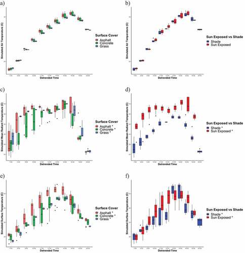
MRT and LST appear to respond differently to land features. For MRT, tree canopies were cooler spots during the day, but then became warm spots after sunset. For LST, the white rooftops, followed by impervious surfaces (roads) were the hottest surface features at 8:00 and 20:00 and trees and other vegetation were the coolest. From 10:00 to 15:00, however, the white rooftops became the coolest surface feature and impervious surfaces became the hottest. MRT and AT simulations do not include buildings. Excluding rooftops, impervious surfaces were consistently hot in all models.

The results of the Kruskal–Wallis test revealed that differences in mean simulated AT were not significantly different by surface type, while they were significant by surface type for both MRT and ST (Supplement 9). Similarly, for sun exposed and shaded sites ST and MRT means were significant at the .05 confidence interval, but not AT (Supplement 10).

Predictive power of RS-LST and shortwave radiation on simulated climate conditions

In order to assess the predictive capacity of RS-LST, we ran a set of regressions with all simulated temperature variables aggregated to 30 m (Table 2). Overall, RS-LST most strongly associated with the simulated LST, MRT, and AT in the evening after sunset, and in all cases that relationship was negative. The strongest relationship was inverse between RS-LST and simulated LST after sunset. The 10:30 MST RS-LST had a weak relationship with simulated LST at 10:00 MST. The strongest positive relationship between RS-LST and any variable was simulated LST at noon, but RS-LST explained less than one third of the variance. During the day, RS-LST predicted more variance in simulated MRTs than LSTs and could explain approximately 40% of the variance for all hours. AT was not correlated with RS-LST except in the evening after sunset and the relationship was negative.

MRT is known to be highly influenced by incoming solar radiation (shade variation), so we ran a second set of regressions with all temperature variables. The incoming solar radiation explained more variation in simulated results than the RS-LST analysis. Incoming solar radiation best explained the temporal change of MRT, with R2 ranging from 0.73 to 0.98. Simulated incoming solar radiation explained approximately 50% of the simulated LST variation at 10:00 and 12:00 MST. Simulated incoming solar radiation has little predictive power over AT.

To implement the multiple linear regression analysis, we aggregated the fine-scale land cover, building height, and ENVI-met simulation results to the 30 m Landsat grid level using the zonal tool in ArcGIS. There are in total 1173 observations (the number of 30 m Landsat pixels in the study area). In the result, land cover variables explained LST the best of the simulated variables, with the highest R2 of 0.89 (Table 3). Buildings and impervious surfaces explained most of the variation in simulated LST for all hours except evening after sunset, for which bare soil was the strongest predictor (−0.94). Trees were a weaker predictor of simulated LST than impervious surfaces. Albedo had a negligible effect on the model.

Different land cover variables explained MRT to a lesser extent. Tree cover and building height were strongest predictors for all hours except noon, for which bare soil and imperviousness were the largest predictors of MRT. Except for 20:00 MST, land cover variables show little association with AT.

Discussion

To better understand the utility of RS-LST in hyper-local urban planning, this study investigated diurnal trends, the predictive capacity of proxy variables, and relationships with urban land features of three field and simulated climate variables: LST, MRT, and AT. Diurnal observations and simulations revealed different trends in LST, MRT, and AT over the course of a day. Consistent with expectations, LST and AT observations were lowest in the morning, peaked around noon (LST) and in the afternoon (AT), and remained relatively high into the evening. This diurnal trend is in line with the UHI and SUHI phenomena and points to the role of impervious surface materials in retaining heat in the late afternoon and evening hours. In contrast, but also expected, MRT observations were comparatively high in unshaded areas, peaked in the afternoon, but cooled down precipitously in the evening around sunset due to the absence of incoming solar radiation. This diurnal trend forefronts the role of sunlight: temperature observations varied widely in the morning because MRT is dependent on full sun exposure versus shade, and observations were low in the evening with no sun.

Compared to field-based and simulated LST, the RS-LST values derived from a single, daytime, 30 m resolution Landsat8 scene under-estimated high and over-estimated low surface temperature values that occurred throughout the day and for the same time of day. This finding is consistent with other studies comparing remote and in situ observations (J. K. Vanos et al., 2016), especially as the performance of LST-retrieval algorithms depends on site context (Sekertekin & Bonafoni, 2020). Uncertainty in the remotely sensed LST data has been chronicled in previous studies: in the single-channel algorithm, the downwelling radiance used to generate the provisional surface temperature product could result in ~0.5°C underestimation on average (USGS, n.d.). This underestimation may be more pronounced over desert and arid regions where the atmospheric relative humidity is low. The mismatch between in situ observed LST and remotely-sensed LST is in part driven by the scale mismatches between the datasets and the relatively coarse, 30 m resolution, RS-LST data, which masks touch-scale urban features (Z.-L. J. K. Vanos et al., 2016). Moreover, peak simulated LST occurred in the afternoon. The Landsat8 image used for this study was taken mid-morning, further attenuating surface temperature readings for the day. As a proxy indicator for surface temperature, therefore, RS-LST generated a modest estimate.

As a predictor of our three climate variables, overall RS-LST was weaker than the model-derived estimate of sunlight/shade. Incoming solar radiation was a better predictor of both simulated LST and MRT than RS-LST, which may be partly driven by the finer scale of analysis, but also the importance of sun exposure in determining high hyper-local variation in climate conditions, including LST (Middel & Krayenhoff, 2019). Although weaker overall, RS-LST was a stronger predictor of simulated MRT than simulated LST. Moreover, the strongest predictive relationships for RS-LST were negative for evening observations: sites that have high RS-LST at 10:30 MST such as barren soil have the coolest night-time MRT. ENVI-met simulations are known to underestimate heat retention. In the simulated results, MRT drops faster than LST around sunset due to the absence of shortwave radiation and stays below AT. At 20:00 MST, the maximum simulated value of is MRT is 26.7◦C compared to 35.6◦C of LST. As expected, AT did not vary much throughout the study area and neither proxy variable held much predictive power.

The observational data enabled for more nuanced exploration of land features and ST. For instance, within one category of surface material, concrete, LST observations were highly varied. Remote sensing-based insights would suggest that LST would be similar within one particular land class because surface material factors such as reflectance would be the same. Variability suggests that factors other than albedo may be influencing LST. One potential hypothesis is that shading from buildings and street trees on concrete sidewalks was driving differences in observed LST. This hypothesis is further supported by the results of the regression analysis that showed a stronger than expected relationship between incoming shortwave radiation (shade variability) and observed LST (Zhang et al., 2019). Another pattern confirmed through high-resolution field and simulation data is that grass effectively lowers ST similar to patterns observable in RS-LST, but does not provide the same cooling benefit for AT or MRT (Lindberg et al., 2016). Additionally, our simulations reveal trees trapping heat in the evening, leading to higher LST values than the background desert, and slightly elevated MRT values. This finding contrasts with conventional remote sensing analysis that typically returns a negative relationship between trees and LST because remote observations assess the tree canopy surface (Rogan et al., 2013; Zhou et al., 2017). Our LST finding contrasts with one study used remote sensing to estimate below canopy LST; it did not find large differences in canopy and below canopy LST, but did find that canopy LST underestimated AT (Cheung et al., 2021). Understanding how different temperature variables respond to below trees and other shade casting canopies varies from the surface temperature of the shade structure itself under different contexts is an important future question for municipal planning. Our study findings potentially add to a growing list of contingent factors and ecosystem service trade-offs to consider in urban tree planting programs and turf grass-based greening (Monteiro, 2017; Roman et al., 2020). Resolving trade-offs among measure, resolution, and time of day associated with a robust analysis of heat conditions will ultimately require a normative discussion of priorities that consider how, when, and by whom space is used.

Our regression analysis of land cover features reveals that conventional land cover classes describing two-dimensional land attributes were a better predictor of simulated LST than MRT. Three-dimensional attributes like building height and tree canopy were better predictors of MRT. This finding is in line with existing scholarship demonstrating the relationship between buildings, trees, and other shade features and MRT (Middel et al., 2021). It also suggests that surfaces are less relevant for predicting thermal comfort than three-dimensional morphology, similar to findings from (Zhang et al., 2019) that three-dimensional urban form is a better predictor of LST than two-dimensional land cover assessments. Additionally, our regression analysis did not find a strong relationship between albedo and simulated LST, moderating findings from a previous study of the site that found a strong relationship between albedo and RS-LST (Turner & Galletti, 2015). This result highlights the difference between conventional remote sensing analysis and hyper-local field and simulated analysis. It also underscores the importance of factors other than surface reflectivity such as evapotranspiration and thermal emittance, which also have a strong influence on surface temperature in hyper-local settings (Sailor, 2014; Taha, 1997).

There are several limitations in our investigation of similarities and differences in the way that different data sets describe microclimate conditions. The simulation did not include the different types of gravel present in the neighborhood due to the complexity of capturing each type. Instead, gravel surface covers were consolidated into a simplified category, sandy loam. Simulation results in these areas are slightly underestimated during the day, as gravel heats up more quickly than soil, and are slightly overestimated at night since gravel cools down more quickly. The ENVI-met simulation results for ST, AT, and MRT by land cover type and sun exposure in Figure 2, while very similar, are not a direct comparison to in-situ observations in Figure 3. Several receptor sites in the ENVI-met simulation were removed from the analysis since those corresponding receptor sites were located on gravel. Additionally, the simulated sun exposure patterns at each of the receptor sites were close, but did not follow the exact observed sun exposure patterns. The remotely sensed data were obtained from a single, daytime image at 30 m resolution at 10 am, so we were unable to assess how well RS-LST derived from other sensors predicted variation in ST, AT, and MRT at the same time of day. Similarly, field data were also collected on one day because of resource and safety concerns related to the physical demands and technical skills required to operate MaRTy. Future studies should include multiple observation days for the same site. Estimates of surface temperature were averaged over a larger spatial unit than field and simulated data. All data are subject to known estimation and simulation biases. For instance, RS-LST estimates for daytime are low, MRT estimates for nighttime are low. To compare data at two different scales, all data were aggregated to 30 m, which potentially increases the strength of predicted relationships in the regression model. Hyper-local conditions are highly context dependent. Our study focused on a single-family residential setting in an arid environment, but the degree to which surfaces versus two-dimensional configuration of those surfaces are predictive of thermal conditions is not ubiquitous across land use (Connors et al., 2013). In addition, the extent to which albedo versus evapotranspiration contribute to cooling is not ubiquitous across climate zones (Georgescu et al., 2014). Future studies should consider the extent to which RS-LST is a proxy across other land use categories and environmental conditions.

Conclusion, future directions, and policy relevance

As a proxy variable for guiding urban heat mitigation efforts, LST has several shortcomings in its capacity to fully explain spatial and diurnal variation in climate conditions and differences between LST, MRT, and AT. These are not simply nuances in the data, but important factors for cities to consider as they plan outdoor space to mitigate heat in the built environment, address regional UHI, protect people from extreme heat exposure, and redress heat disparities in low income and communities of color. Cities have multiple heat problems to solve and will require hyper-local data to consider multiple measures of temperature across different contexts. Currently, such data sets are not widely available to cities because it is fieldwork and modeling intensive. Future work should move toward deriving better regional estimates of measures such as MRT and, simultaneously, determining which case-study insights are transferable under what conditions. Until such technology is made widely available, increasing urban climate literacy among planners and policymakers so that discussions about urban cooling clarify which heat problem is being discussed, which temperature type is the appropriate metric, and a discussion of trade-offs with other heat-related goals is a good first step (Ladd Keith et al., 2021). Another step for urban climate scientists is to develop guidelines or typologies that help decision-makers select context-appropriate cooling interventions, when field-intensive assessments of ST, AT, and MRT are not feasible.

Although RS-LST maps are widely used by cities (L. Keith et al., 2019), municipalities might reconsider the extent to which the regional UHI concept is meaningful in guiding action at hyper-local scales (Martilli et al., 2020). This is especially salient as cities consider using high albedo impervious surfaces to combat UHI. An Environmental Protection Agency (EPA) report conducted in conjunction with the Lawrence Berkeley Lab summarizes the benefits and drawbacks of reflective surfaces, stating, ‘Using reflective of permeable pavements where people congregate or children play can provide localized comfort benefits through lower surface and near-surface air temperatures,’ (pg. 24). Our findings, and other urban climate studies on high albedo previous surfaces in hyper-local contexts, suggest otherwise (Middel et al., 2020; Salata et al., 2015; Saneinejad et al., 2014). Increasing surface albedo on previous surfaces without considering multiple climate regulation services provided by impervious surfaces, the role of three-dimensional urban environment, and the central role of shade, will not necessarily provide hyper-local thermal comfort improvements and, potentially, increases human heat load. In other words, ‘cool surfaces’ cannot be considered a substitute for other cooling interventions.

This study underscores the importance of urban heat literacy for climate adaptation. Extreme heat events and the urban heat island are rapidly becoming mainstream policy lexicon as climate change forces all cities – even in temperature environments – to confront urban heat. Thermal comfort and the difference between LST, MRT, and AT are not as readily understood. It is incumbent on the urban climate community to make clear that heat is a multifaceted phenomenon and there is no one-size-fits all solution, especially in hyper-local settings.

Disclosure statement

No potential conflict of interest was reported by the author(s).

Supplementary materials

Supplemental data for this article can be accessed here.

References

- Aram, F., Higueras García, E., Solgi, E., & Mansournia, S. (2019). Urban green space cooling effect in cities. Heliyon, 5(4), e01339. https://doi.org/10.1016/j.heliyon.2019.e01339
- Arnfield, A.J. (2003). Two decades of urban climate research: A review of turbulence, exchanges of energy and water, and the urban heat Island. International Journal of Climatology, 23(1), 1–26. https://doi.org/10.1002/joc.859
- Bowler, D.E., Buyung-Ali, L., Knight, T.M., & Pullin, A.S. (2010). Urban greening to cool towns and cities: A systematic review of the empirical evidence. Landscape and Urban Planning, 97(3), 147–155. https://doi.org/10.1016/j.landurbplan.2010.05.006
- Bruse, M. (2020). ENVI-met4.4.6. [Software]. http://www.envi-met.com
- Bruse, M., & Fleer, H. (1998). Simulating surface–plant–air interactions inside urban environments with a three dimensional numerical model. Environmental Modelling & Software, 13(3), 373–384. https://doi.org/10.1016/S1364-8152(98)00042-5
- Buyantuyev, A., Wu, J., & Gries, C. (2010). Multiscale analysis of the urbanization pattern of the Phoenix metropolitan landscape of USA: Time, space and thematic resolution. Landscape and Urban Planning, 94(3), 206–217. https://doi.org/10.1016/j.landurbplan.2009.10.005
- Chambers, J. (2020). Global and cross-country analysis of exposure of vulnerable populations to heatwaves from 1980 to 2018. Climatic Change, 163(1), 539–558. https://doi.org/10.1007/s10584-020-02884-2
- Cheung, P.K., Jim, C.Y., & Hung, P.L. “Preliminary Study on the Temperature Relationship at Remotely-Sensed Tree Canopy and below-Canopy Air and Ground Surface.” Building and Environment 204 (October 15, 2021): 108169. https://doi.org/10.1016/j.buildenv.2021.108169
- Connors, J.P., Galletti, C.S., & Chow, W.T.L. (2013). Landscape configuration and urban heat Island effects: Assessing the relationship between landscape characteristics and land surface temperature in Phoenix, Arizona. Landscape Ecology, 28(2), 271–283. https://doi.org/10.1007/s10980-012-9833-1
- Cook, M.J. (2014). Atmospheric Compensation for a Landsat Land Surface Temperature Product [Ph.D., Rochester Institute of Technology]. ProQuest Dissertation Publishing. https://www.proquest.com/docview/1649232520/abstract/DD11F3059A4241F7PQ/1
- Crewe, K., Brazel, A., & Middel, A. (2016, November). Desert New Urbanism: Testing for Comfort in Downtown Tempe, Arizona. Journal of Urban Design, 21(6), 746–763. https://doi.org/10.1080/13574809.2016.1187558
- Daniel, M., Lemonsu, A., & Viguié, V. (2018). Role of watering practices in large-scale urban planning strategies to face the heat-wave risk in future climate. Urban Climate, 23, 287–308. https://doi.org/10.1016/j.uclim.2016.11.001
- Deilami, K., Kamruzzaman, M., & Liu, Y. (2018). Urban heat Island effect: A systematic review of spatio-temporal factors, data, methods, and mitigation measures. International Journal of Applied Earth Observation and Geoinformation, 67, 30–42. https://doi.org/10.1016/j.jag.2017.12.009
- Di Liberto, T. (2021, June). Astounding heat obliterates all-time records across the Pacific Northwest and Western Canada in June 2021 | NOAA Climate.gov. NOAA. https://www.climate.gov/news-features/event-tracker/astounding-heat-obliterates-all-time-records-across-pacific-northwest
- Erell, E., Pearlmutter, D., Boneh, D., & Kutiel, P.B. (2014). Effect of high-albedo materials on pedestrian heat stress in urban street canyons. Urban Climate, 10, 367–386. https://doi.org/10.1016/j.uclim.2013.10.005
- Georgescu, M., Morefield, P.E., Bierwagen, B.G., & Weaver, C.P. (2014). Urban adaptation can roll back warming of emerging megapolitan regions. Proceedings of the National Academy of Sciences, 111(8), 2909–2914. https://doi.org/10.1073/pnas.1322280111
- Getis, A., & Ord, J.K. (1992). The Analysis of Spatial Association by Use of Distance Statistics. Geographical Analysis, 24(3), 189–206. https://doi.org/10.1111/j.1538-4632.1992.tb00261.x
- Google Earth (7.3.2.5776). (2019). https://earth.google.com/web/. [Accessed 2019]
- Google Earth Engine (2019). National Agriculture Imagery Program. https://developers.google.com/earth-engine/datasets/catalog/USDA_NAIP_DOQQ. [Accessed 2019]
- Häb, K., Ruddell, B.L., & Middel, A. (2015). Sensor lag correction for mobile urban microclimate measurements. Urban Climate, 14, 622–635. https://doi.org/10.1016/j.uclim.2015.10.003
- Hoffman, J.S., Shandas, V., & Pendleton, N. (2020). The Effects of Historical Housing Policies on Resident Exposure to Intra-Urban Heat: A Study of 108 US Urban Areas. Climate, 8(1), 12. https://doi.org/10.3390/cli8010012
- Imran, H.M., Kala, J., Ng, A.W.M., & Muthukumaran, S. (2018). Effectiveness of green and cool roofs in mitigating urban heat Island effects during a heatwave event in the city of Melbourne in southeast Australia. Journal of Cleaner Production, 197, 393–405. https://doi.org/10.1016/j.jclepro.2018.06.179
- Jones, B., O’Neill, B.C., McDaniel, L., McGinnis, S., Mearns, L.O., & Tebaldi, C. (2015). Future population exposure to US heat extremes. Nature Climate Change, 5(7), 652–655. https://doi.org/10.1038/nclimate2631
- Keith, L., Meerow, S., Hondula, D.M., Turner, V.K., & Arnott, J.C. (2021, October). Deploy Heat Officers, Policies and Metrics. Nature, 598 (7879), 29–31. https://doi.org/10.1038/d41586-021-02677-2
- Keith, L., Meerow, S., & Wagner, T. (2019). Planning for Extreme Heat: A Review. Journal of Extreme Events, 6( 03n04), 2050003. https://doi.org/10.1142/S2345737620500037
- Kotharkar, R., & Bagade, A. Evaluating Urban Heat Island in the Critical Local Climate Zones of an Indian City. Landscape and Urban Planning, 169, January 1, 2018, 92–104. https://doi.org/10.1016/j.landurbplan.2017.08.009
- Krüger, EL., Minella, FO., and Matzarakis, A. (2014). Comparison of different methods of estimating the mean radiant temperature in outdoor thermal comfort studies. International Journal of Biometeorology, 58, 1727–1737.
- Kruskal, W.H., & Wallis, W.A. Use of Ranks in One-Criterion Variance Analysis. Journal of the American Statistical Association, 47 (260), December 1, 1952, 583–621. https://doi.org/10.1080/01621459.1952.10483441
- Laraby, K.G., & Schott, J.R. (2018). Uncertainty estimation method and Landsat 7 global validation for the Landsat surface temperature product. Remote Sensing of Environment, 216, 472–481. https://doi.org/10.1016/j.rse.2018.06.026
- Li, X., Li, W., Middel, A., Harlan, S.L., Brazel, A.J., & Turner, B.L. (2016). Remote sensing of the surface urban heat Island and land architecture in Phoenix, Arizona: Combined effects of land composition and configuration and cadastral–demographic–economic factors. Remote Sensing of Environment, 174, 233–243. https://doi.org/10.1016/j.rse.2015.12.022
- Liao, W., Hong, T., & Heo, Y. (2021). The effect of spatial heterogeneity in urban morphology on surface urban heat Islands. Energy and Buildings, 244, 111027. https://doi.org/10.1016/j.enbuild.2021.111027
- Lindberg, F., Onomura, S., & Grimmond, C.S.B. September 1, 2016. Influence of Ground Surface Characteristics on the Mean Radiant Temperature in Urban Areas. International Journal of Biometeorology, https://doi.org/10.1007/s00484-016-1135-x 60 9, 1439–1452.
- Mackey, C., Galanos, T., Norford, L., Roudsari, M.S., & Architects, P. (2017). Wind, Sun, Surface Temperature, and Heat Island: Critical Variables for High-Resolution Outdoor Thermal Comfort. International Building Performance Simulation Association. (pp. 9).
- Martilli, A., Krayenhoff, E.S., & Nazarian, N. (2020). Is the Urban Heat Island intensity relevant for heat mitigation studies? Urban Climate, 31, 100541. https://doi.org/10.1016/j.uclim.2019.100541
- Meadow, A.M., LeRoy, S., Weiss, J., & Keith, L. (2019). Climate Profile for The Highlands at Dove Mountain (p. 35). University of Arizona. Climate Assessment for the Southwest (CLIMAS). https://climas.arizona.edu/sites/default/files/CLIMAS%20Highlands-Dove-Mountain-FINAL.pdf
- Meehl, G.A., & Tebaldi, C. (2004). More Intense, More Frequent, and Longer Lasting Heat Waves in the 21st Century. Science, 305(5686), 994–997. https://doi.org/10.1126/science.1098704
- Meerow, S., and Keith, L. (2021). Planning for extreme heat: A national survey of U.S. planners. Journal of the American Planning Association. https://doi.org/10.1080/01944363.2021.1977682
- Middel, A., Alkhaled, S., Schneider, F.A., Hagen, B., & Coseo, P. (2021). 50 Grades of Shade. Bulletin of the American Meteorological Society, 1(aop), 1–35. https://doi.org/10.1175/BAMS-D-20-0193.1
- Middel, A., Häb, K., Brazel, A.J., Martin, C.A., & Guhathakurta, S. (2014). Impact of urban form and design on mid-afternoon microclimate in Phoenix Local Climate Zones. Landscape and Urban Planning, 122, 16–28. https://doi.org/10.1016/j.landurbplan.2013.11.004
- Middel, A., & Krayenhoff, E.S. (2019). Micrometeorological determinants of pedestrian thermal exposure during record-breaking heat in Tempe, Arizona: Introducing the MaRTy observational platform. Science of the Total Environment, 687, 137–151. https://doi.org/10.1016/j.scitotenv.2019.06.085
- Middel, A., Selover, N., Hagen, B., & Chhetri, N. (2016). Impact of shade on outdoor thermal comfort—A seasonal field study in Tempe, Arizona. International Journal of Biometeorology, 60(12), 1849–1861. https://doi.org/10.1007/s00484-016-1172-5
- Middel, A., Turner, V.K., Schneider, F.A., Zhang, Y., & Stiller, M. (2020). Solar reflective pavements—A policy panacea to heat mitigation? Environmental Research Letters, 15(6), 064016. https://doi.org/10.1088/1748-9326/ab87d4
- Mohajerani, A., Bakaric, J., & Jeffrey-Bailey, T. (2017). The urban heat Island effect, its causes, and mitigation, with reference to the thermal properties of asphalt concrete. Journal of Environmental Management, 197, 522–538. https://doi.org/10.1016/j.jenvman.2017.03.095
- Monteiro, J.A. (2017, August 1). Ecosystem Services from Turfgrass Landscapes. Urban Forestry & Urban Greening, Special Feature: TURFGRASS, 26, 151–157. https://doi.org/10.1016/j.ufug.2017.04.001
- Moule & Polyzoides. Civano New Town | Moule & Polyzoides. (n.d.). Retrieved from November 19, 2021, https://mparchitects.com/site/projects/civano-new-town
- Oke, T.R. (1982). The energetic basis of the urban heat Island. Quarterly Journal of the Royal Meteorological Society, 108(455), 1–24. https://doi.org/10.1002/qj.49710845502
- OpenStreetMap contributors. (2019). https://planet.openstreetmap.org
- Oxoli, D., & Prestifilippo, G. (2017). Hotspot Analysis: An experimental Python plugin to enable LISA mapping into QGIS. Proceedings of FOSS4G Europe 2017. https://re.public.polimi.it/handle/11311/1046656#.YQXf7FNKjvU
- QGIS Development Team (Version 3.14). (2019). QGIS Geographic Information System. Open Source Geospatial Foundation Project. http://qgis.osgeo.org”
- Rogan, J., Ziemer, M., Martin, D., Ratick, S., Cuba, N., & DeLauer, V. (2013). The impact of tree cover loss on land surface temperature: A case study of central Massachusetts using Landsat Thematic Mapper thermal data. Applied Geography, 45, 49–57. https://doi.org/10.1016/j.apgeog.2013.07.004
- Roman, L.A., Conway, T.M., Eisenman, T.S., Koeser, A.K., Ordóñez Barona, C., Locke, D.H., Jenerette, G.D., Östberg, J., & Vogt, J. (2020). Beyond ‘trees are good’: Disservices, management costs, and tradeoffs in urban forestry. Ambio. https://doi.org/10.1007/s13280-020-01396-8
- Roussel, J.-R., Auty, D., Coops, N.C., Tompalski, P., Goodbody, T.R.H., Meador, A.S., Bourdon, J.-F., de Boissieu, F., & Achim, A. (2020). lidR: An R package for analysis of Airborne Laser Scanning (ALS) data. Remote Sensing of Environment, 251, 112061. https://doi.org/10.1016/j.rse.2020.112061
- Roussel, J.-R., documentation), D. A. (Reviews the, features), F. D. B. (Fixed bugs and improved catalog, segment_snags()), A. S. M. (Implemented wing2015() for, track_sensor()), B. J.-F. (Contributed to R. for, track_sensor()), G. D. (Implemented G. for, & management), L. S. (Contributed to parallelization. (2021). lidR: Airborne LiDAR Data Manipulation and Visualization for Forestry Applications (3.1.4) [Computer software]. https://CRAN.R-project.org/package=lidR
- Sailor, D.J. (2014). A holistic view of the effects of urban heat Island mitigation Lehmann, Steffen. In Low Carbon Cities. London: Routledge.
- Salata, F., Golasi, I., de Lieto Vollaro, R., and de Lieto Vollaro, A. (2016). Outdoor thermal comfort in the Mediterranean area. A transversal study in Rome, Italy. Building and Environment, 96, 46–61.
- Salata, F., Golasi, I., de Vollaro, A.L., & de Vollaro, R.L. (2015). How high albedo and traditional buildings’ materials and vegetation affect the quality of urban microclimate. A case study. Energy and Buildings, 99, 32–49. https://doi.org/10.1016/j.enbuild.2015.04.010
- Saneinejad, S., Moonen, P., & Carmeliet, J. (2014). Comparative assessment of various heat Island mitigation measures. Building and Environment, 73, 162–170. https://doi.org/10.1016/j.buildenv.2013.12.013
- Santamouris, M. (2013). Using cool pavements as a mitigation strategy to fight urban heat Island—A review of the actual developments. Renewable and Sustainable Energy Reviews, 26, 224–240. https://doi.org/10.1016/j.rser.2013.05.047
- Sekertekin, A., & Bonafoni, S. (2020). Land Surface Temperature Retrieval from Landsat 5, 7, and 8 over Rural Areas: Assessment of Different Retrieval Algorithms and Emissivity Models and Toolbox Implementation. Remote Sensing, 12(2), 294. https://doi.org/10.3390/rs12020294
- Sheridan, S.C., Dixon, P.G., Kalkstein, A.J., & Allen, M.J. (2021). Recent Trends in Heat-Related Mortality in the United States: An Update through 2018. Weather, Climate, and Society, 13(1), 95–106. https://doi.org/10.1175/WCAS-D-20-0083.1
- Stewart, I.D., & Oke, T.R. (2012). Local Climate Zones for Urban Temperature Studies. Bulletin of the American Meteorological Society, 93(12), 1879–1900. https://doi.org/10.1175/BAMS-D-11-00019.1
- Synnefa, A., Santamouris, M., & Apostolakis, K. (2007). On the development, optical properties and thermal performance of cool colored coatings for the urban environment. Solar Energy, 81(4), 488–497. https://doi.org/10.1016/j.solener.2006.08.005
- Taha, H. (1997). Urban climates and heat Islands: Albedo, evapotranspiration, and anthropogenic heat. Energy and Buildings, 25(2), 99–103. https://doi.org/10.1016/S0378-7788(96)00999-1
- Thomas, G., Sherin, A.P., Ansar, S., & Zachariah, E.J. “Analysis of Urban Heat Island in Kochi, India, Using a Modified Local Climate Zone Classification.” Procedia Environmental Sciences, Urban Environmental Pollution 2013 – Creating Healthy, Livable Cities, 21 (January 1, 2014): 3–13. https://doi.org/10.1016/j.proenv.2014.09.002
- Turner, V.K., & Galletti, C.S. (2015). Do Sustainable Urban Designs Generate More Ecosystem Services? A Case Study of Civano in Tucson, Arizona. The Professional Geographer, 67(2), 204–217. https://doi.org/10.1080/00330124.2014.922021
- Turner, VK., and Galletti, CS. 2014. Do Sustainable Urban Designs Generate More Ecosystem Services? A Case Study of Civano in Tucson, Arizona. The
- USGS. (n.d.). Landsat Science Products. Landsat Provisional Surface Temperature. Retrieved November 16, 2021, from https://www.usgs.gov/core-science-systems/nli/landsat/landsat-provisional-surface-temperature?qt-science_support_page_related_con=0#qt-science_support_page_related_con
- Vanos, J.K., Middel, A., McKercher, G.R., Kuras, E.R., & Ruddell, B.L. (2016). Hot playgrounds and children’s health: A multiscale analysis of surface temperatures in Arizona, USA. Landscape and Urban Planning, 146, 29–42. https://doi.org/10.1016/j.landurbplan.2015.10.007
- Vanos, J.K., Warland, J.S., Gillespie, T.J., & Kenny, N.A. Review of the Physiology of Human Thermal Comfort While Exercising in Urban Landscapes and Implications for Bioclimatic Design. International Journal of Biometeorology, 54 (4), July 1, 2010, 319–334. https://doi.org/10.1007/s00484-010-0301-9
- Voogt, J.A., & Oke, T.R. (2003). Thermal remote sensing of urban climates. Remote Sensing of Environment, 86(3), 370–384. https://doi.org/10.1016/S0034-4257(03)00079-8
- Willmott, C.J. (1981). On the Validation of Models. Physical Geography, 2(2), 184–194. https://doi.org/10.1080/02723646.1981.10642213
- Yang, J., Wang, Y., Xiu, C., Xiao, X., Xia, J., & Jin, C. Optimizing Local Climate Zones to Mitigate Urban Heat Island Effect in Human Settlements. Journal of Cleaner Production, 275, December 1, 2020, 123767. https://doi.org/10.1016/j.jclepro.2020.123767
- Zhang, Y., Middel, A., & Turner, B.L. (2019). Evaluating the effect of 3D urban form on neighborhood land surface temperature using Google Street View and geographically weighted regression. Landscape Ecology, 34(3), 681–697. https://doi.org/10.1007/s10980-019-00794-y
- Zhou, W., Wang, J., & Cadenasso, M.L. (2017). Effects of the spatial configuration of trees on urban heat mitigation: A comparative study. Remote Sensing of Environment, 195, 1–12. https://doi.org/10.1016/j.rse.2017.03.043