Hyperspectral NIR time series imaging used as a new method for estimating the moisture content dynamics of thermally modified Scots pine

ABSTRACT

The purpose of this research is to develop a method for estimating the spatially and temporally resolved moisture content of thermally modified Scots pine (Pinus sylvestris) using remote sensing. Hyperspectral time series imaging in the NIR wavelength region (953–2516 nm) was used to gather information about the absorbance of eight thermally modified pine samples each minute as they dried during a period of approximately 20 h. After preprocessing the collected spectral data and identifying an appropriate wavelength selection, partial least squares regression (PLS) was used to map the absorbance data of each pine sample to a distribution of moisture contents within the samples at different time steps during the drying process. To enable separate studying and comparison of the drying dynamics taking place within the early- and latewood regions of the pine samples, the collected images were spatially segmented to separate between early- and latewood pixels. The results of the study indicate that the 1966–2244 nm region of a NIR spectrum, when preprocessed with extended multiplicative scatter correction and first order derivation, can be used to model the average moisture content of thermally modified pine using PLS. The methods presented in this paper allows for estimation and visualization of the intrasample spatial distribution of moisture in thermally modified pine wood.

KEYWORDS:

• Hyperspectral imaging
• thermally modified pine
• TMT
• hyperspectral time series
• moisture content
• PLS

1. Introduction

Altering the properties of timber using heat is a practice that dates back thousands of years (Brelid 2013). It is well known that exposing timber to high temperatures in an oxygen deficient environment—i.e. thermally modifying it—can increase the dimensional stability of the wood and improve its resistance towards moisture-related inconveniences caused by fungi and mold growth (Cirule et al. 2015, Dunningham and Sargent 2015, Sandberg and Kutnar 2016) such as wood discoloration, visible mold growth or unpleasant smelling. More recently, along with an increased demand for environmentally friendly construction materials, thermally modified timber (TMT) has rapidly gained popularity in applications such as claddings, decks and floors partly due to the nontoxic and eco-friendly nature of the treatment (Cirule et al. 2015, Dunningham and Sargent 2015). It is known that the equilibrium moisture content (EMC) of wood decreases when undergoing thermal modification (Hill 2006, Esteves and Pereira 2009). It is also known that as wood dries, gradients of varying moisture content are formed in the wood structure in both the radial, tangential and longitudinal direction (Edward 1957). Internal differences in the moisture content of a wood board cause swelling and contraction to occur at different rates within the board, which in turn leads to tensile stresses in the wood which may cause several undesired consequences: for instance, it may cause the wood, or coatings applied to the wood surface, to crack (Schweitzer 1999), or it may cause the wood to deform, sometimes permanently (Edward 1957). Methods enabling the spatial distribution of moisture within a wood board to be quantified is therefore of interest within wood sciences. Previous studies have used magnetic resonance imaging (MRI) to study the distribution of moisture within both thermally modified (Kekkonen et al. 2014, Javed et al. 2015) and unmodified (Hameury and Sterley 2006) pine. The spatial resolution of MRI is however still relatively low, and such instruments are large and difficult to use outdoors to survey existing structures. Near infrared (NIR) spectroscopy has become a popular tool in wood sciences due to its ability of nondestructively allowing several useful wood properties to be characterized. Previous studies have shown that the density of wood (Fujimoto et al. 2012), the mechanical stress of wood (Sandak et al. 2013), the geographical growth region of wood (Sandak et al. 2010) and its moisture content (Watanabe et al. 2011) can all be approximated from nondestructive NIR measurements of the sample. Using hyperspectral imaging, as opposed to traditional point based NIR measurements, allows the NIR data to be used to nondestructively approximate the spatial distribution of wood properties. Kobori et al. demonstrated that hyperspectral imaging in the vis-NIR wavelength region can be used together with multivariate regression as a viable means of determining the spatial distribution of moisture content in unmodified pine (Kobori et al. 2013). Myronycheva et al. used hyperspectral NIR imaging to exploratively study the chemical composition of thermally modified pine using principal component analysis (Myronycheva et al. 2018).

In the present study, the feasibility of using hyperspectral imaging in the near infrared region (953–2516 nm) to estimate the moisture content distribution of thermally modified pine is evaluated. The ambition of the study is to develop a multivariate regression model capable of nondestructively estimating the spatial distribution of moisture in thermally modified pine samples based on the individual spectra of each pixel of a sample. Partial least squares regression (PLS) will be used to calibrate a regression vector which maps the spectra of the pine samples to a corresponding moisture content. The predicted distributions will then be spatially segmented such that separate estimates are obtained of the moisture content within the early- and latewood regions of each samples. To ensure that the developed model can accurately predict the moisture content of samples at a wide variety of different moisture contents, hyperspectral time series imaging will be used to gather spectral measurements of each sample on a minute-by-minute basis as the samples dry over the course of a day. Whilst hyperspectral cameras cannot be used to measure radial moisture variations in a sample (due to the limited surface penetration depth of the radiation), the relatively high spatial resolution offered by such cameras allow for a detailed view of the tangential and longitudinal variations at the surface.

2. Materials & methods

2.1. Sample preparation & image acquisition

Eight thermally modified boards of Scots pine (Pinus sylvestris) were planed to ensure surface flatness and cut into samples of dimension 18 × 100 × 280 mm. The boards were bought at a local (20 km south of Oslo, Norway) lumberyard and were manufactured by Moelven. The pine originated from a forest in Finland and the thermal modification was performed in Estonia (Tallinn) at 210–215°C for a duration of 46 h according to the ThermoWood method. After being cut, the eight samples were dried at 103°C for 120 h to ensure that only chemically bound moisture resided in the samples. The dryness of the samples was verified by repeatedly measuring the weight of the samples and confirming that their weight had stabilized before removing them from the oven, at which point the oven-dry weight of each sample was recorded and we assumed that there was no free water left in the sample.

In addition to the dry weight, the average annual ring distance ${\text{Å}}_{\overline{x}}$ of each sample was measured in the radial direction (calculated according Section 8 of the SKANORM 2 method (Bohumil 1992)) and a dry density ${\rho }_0$ was calculated for every sample. When establishing the dry density of our samples, the original volume of 18 × 100 × 280 mm was used as dry volume since any shrinkage which may have occurred during drying was too small for us to reliably measure.

After the dry weights were established, the samples were fully submerged in tap water for a period of approximately one and a half months. After the soaking period, the samples were one at a time taken from the water and placed on a digital scale which in turn was placed on a translation stage situated underneath a hyperspectral camera as can be seen depicted in Figure 1.

Figure 1. Illustration of experimental setup. A drying wood sample is positioned on a digital scale which in turn is situated under a hyperspectral push-broom camera and illuminated with halogen spotlights. Figure from (Stefansson et al. 2019a).

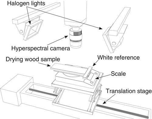
The hyperspectral line scan camera (HySpex SWIR-384 manufactured by Norsk Elektro Optikk, Skedsmokorset, Norway) situated above the sample was automated to scan each sample every minute for a period of roughly 21.5 h as the pine dried. During the first hour or so a film of free water was still present on the surface of some samples which distorted the measured spectra and partly concealed the spectra of the pine sample. The first one hundred images (i.e. the data from the first 100 min of drying) from each sample’s time series was therefore removed from the dataset. The hyperspectral time series data used in the study consists in 1196 images per pine sample, depicting the samples between 1.5 and 21.5 h of drying. The room the image acquisition/drying took place in was conditioned to be approximately 21°C. For every image taken, the corresponding sample weight was also registered. Using the preestablished dry weight, the average moisture content (MC) of each pine sample was calculated for each time point during the drying process based on the instantaneous scale reading using the relation (Kobori et al. 2013):(1) $\mathrm{M}\mathrm{C}=\frac{w_{\mathrm{w}\mathrm{e}\mathrm{t}\mathrm{w}\mathrm{o}\mathrm{o}\mathrm{d}}-w_{\mathrm{d}\mathrm{r}\mathrm{y}\mathrm{w}\mathrm{e}\mathrm{i}\mathrm{g}\mathrm{h}\mathrm{t}}}{w_{\mathrm{d}\mathrm{r}\mathrm{y}\mathrm{w}\mathrm{e}\mathrm{i}\mathrm{g}\mathrm{h}\mathrm{t}}}$(1) where $w_{\mathrm{w}\mathrm{e}\mathrm{t}\mathrm{w}\mathrm{o}\mathrm{o}\mathrm{d}}$ represents the weight of the drying pine sample and $w_{\mathrm{d}\mathrm{r}\mathrm{y}\mathrm{w}\mathrm{e}\mathrm{i}\mathrm{g}\mathrm{h}\mathrm{t}}$ represents the predetermined dry weight of the same sample. The outcome of Equation 1(1) $\mathrm{M}\mathrm{C}=\frac{w_{\mathrm{w}\mathrm{e}\mathrm{t}\mathrm{w}\mathrm{o}\mathrm{o}\mathrm{d}}-w_{\mathrm{d}\mathrm{r}\mathrm{y}\mathrm{w}\mathrm{e}\mathrm{i}\mathrm{g}\mathrm{h}\mathrm{t}}}{w_{\mathrm{d}\mathrm{r}\mathrm{y}\mathrm{w}\mathrm{e}\mathrm{i}\mathrm{g}\mathrm{h}\mathrm{t}}}$(1) describes the amount of water contained in a sample compared to the weight of its dry matter expressed as a percentage. For instance, applying Equation 1 to an oven-dried sample would yield 0%. Whereas a moisture content of 100% would indicate that the weight of the water in the sample is equal to the weight of the same sample in an oven-dried state. Table I provides a summary of each sample’s recorded dry weight, average annual ring distance, dry density, together with highest, lowest, range, average and standard deviation of the calculated moisture content during the drying process.

Table I. Dry weights, average annual ring distance (Å${}_{\overline{\mathrm{x}}}$), dry density (${\rho }_0$), initial moisture content (MC_High), final moisture content (MC_Low), difference between highest and lowest moisture content (MC_Range), average moisture content (MC_µ) and standard deviation of moisture content (MC_σ) of all samples in the study.

Sample	Dry weight	Å${}_{\overline{x}}$	${\rho }_0$	MCHigh	MCLow	MCRange	MCµ	MCσ
S1	188.9 g	2.8 mm	375 kg/m³	73.7%	44.1%	29.5%	56.0%	8.2%
S2	187.0 g	3.1 mm	371 kg/m³	66.9%	38.9%	28.1%	49.4%	7.6%
S3	202.2 g	2.2 mm	401 kg/m³	80.6%	53.2%	27.4%	64.2%	7.2%
S4	211.8 g	2.2 mm	420 kg/m³	63.3%	33.9%	29.4%	44.1%	7.8%
S5	185.8 g	3.7 mm	369 kg/m³	85.4%	47.1%	38.3%	61.0%	10.3%
S6	193.5 g	2.7 mm	384 kg/m³	70.0%	40.2%	29.8%	51.6%	8.2%
S7	190.7 g	3.0 mm	378 kg/m³	77.5%	45.3%	32.3%	57.2%	8.7%
S8	205.5 g	3.0 mm	408 kg/m³	65.1%	35.6%	29.5%	46.6%	8.0%

The hyperspectral camera registered 288 equally spaced bands in the 953–2516 nm range. The spatial resolution of the region of interest of each sample was 801 × 335 pixels. The complete dimensions of the collected hyperspectral dataset is therefore 801 × 335 × 288 × 1196 × 8 (rows x columns x spectral bands x time x sample). Which equates to roughly 5.3 terabytes of spectral intensity data when stored in double-precision format. The region of interest extracted out from each hyperspectral image included roughly 87 mm of the width of each board and 209 mm of the length, centered around the middle of the board. The spatial size of each pixel corresponds to 0.227 × 0.227 mm.

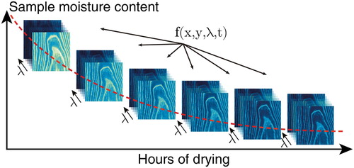
The resulting structure of the experimentally collected data for each sample can be seen conceptually illustrated in Figure 2: each sample is associated with its own four-dimensional hyperspectral time series as well as a one-dimensional time series of its average moisture content.

Figure 2. Illustration of hyperspectral time series data of a drying thermally modified pine sample. The spectral signal of the pine sample is resolved through both time and space. At each time step the average moisture content of the sample is known. Figure from (Stefansson et al. 2019a).

2.2. Early-/latewood image segmentation

To allow for separate estimates to be obtained of the moisture content within early- and latewood regions of a sample during the drying process, the pixels of each hyperspectral image was categorized according to wood type belonging. Wood is a notoriously inhomogeneous material and the seasonal growth patterns takes many, sometimes relatively complex, forms which makes manual segmentation tedious and nontrivial. To enable semi-automatic segmentation of the dataset we employed the principal component analysis-based segmentation technique introduced by Smeland et al. (2016) for discriminating between early- and latewood pixels within our hyperspectral images. The method consists in performing principal component analysis (PCA) on a hyperspectral image and then forming a histogram from the resulting scores associated with one of the principal components. Two thresholds are then placed in the histogram, and datapoints below the lower threshold are classified as earlywood whereas datapoints above the higher threshold are classified as latewood.

2.3. Normalization & linearization of raw spectral signal

The spectrally resolved light intensity images $I\left(\lambda \right)$ registered by the hyperspectral camera were initially converted into reflectance units $R\left(\lambda \right)$, relative to a Spectralon white reference plate included in each image, according to(2) $R\left(\lambda \right)=\frac{I\left(\lambda \right)-I_d\left(\lambda \right)}{I_0\left(\lambda \right)-I_d\left(\lambda \right)}.$(2)

In Equation 2, $I_0\left(\lambda \right)$ represents the measured light intensity of the Spectralon white reference and $I_{\mathrm{d}}\left(\lambda \right)$ represents the dark signal of each image (signal captured with the camera shutter closed). The reflectance images were then transformed into apparent absorbance $A\left(\lambda \right)$ in accordance with Lambert Beer’s law (Rinnan et al. 2009):(3) $A\left(\lambda \right)={\log }_{10}\left(1/R\left(\lambda \right)\right).$(3)

2.4. Regression & data division

The hyperspectral time series data was spatially averaged to obtain one spectrum per image. The data was then reshaped into a two-dimensional matrix $X$ with observations of samples at various time points along the rows and wavelengths along the columns. The average moisture content of each sample and time step—the response values of the dataset—were placed in a one-dimensional vector $y$ such that the rows of $y$ correspond to the same sample and point in time as the rows of $X$. 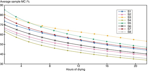The average moisture content of each sample for each time step ($y$) is shown in Figure 3. A partial least squares regression model was calibrated which mapped the average spectra of the wood samples ($X$) to the average measured moisture content ($y$).

Figure 3. Calculated average moisture content of all thermally modified pine samples in the study during the drying period.

In order for the spectra observed at the surface of the pine to be able to predict the bulk moisture content of the sample, the moisture distribution should be homogeneous throughout the thickness of the sample, such that what is observed at the surface of a sample is representative of what occurs throughout its thickness. As wood is inhomogeneous this is naturally never entirely the case. The assumption in our mapping from $X$ to $y$ is that the relation between inner moisture content and surface moisture content is stable enough to allow for useful approximations of the moisture distribution to indirectly be made by studying only the surface of the sample.

To test the developed model’s ability to generalize to new unseen data, the hyperspectral time series of two samples, S5 and S2, were randomly chosen and withheld from the calibration procedure. After calibrating the model on the remaining six samples’ time series the model was applied to the data from the two withheld time series (2 × 1196 images) to validate its performance on new data. In total, 7176 hyperspectral images were included in the training set and 2392 images were included in the validation set.

To enhance the performance of the PLS model, spectral preprocessing and wavelength selection was applied to the measured absorbance data. In order to identify a spectral preprocessing technique that would yield a low prediction error in the PLS regression, a grid search over different common NIR preprocess methods was therefore conducted. In addition to the unprocessed absorbance spectra, the methods included in this search were: Savitzky–Golay derivation (Savitzky and Golay 1964) of first, second and third order, Multiplicative Scatter Correction (Geladi and MacDougall 1985) (MSC), Standard Normal Variate (Barnes et al. 1989) (SNV) and Extended Multiplicative Scatter Correction (Martens and Stark 1991) (EMSC) as well as pairwise combinations of these methods. For each of the preprocessing methods a PLS model was calibrated and cross-validated with 10-fold cross-validation. The preprocessing technique resulting in the lowest cross-validated root-mean-squared-error (RMSEcv) was chosen for the final model.

Once a suitable preprocessing technique was identified, the preprocessed data was subjected to variable selection in order to further enhance the model’s performance by eliminating irrelevant or noisy wavelengths. Forward selection, backwards elimination, interval PLS (Nørgaard et al. 2000) (iPLS) in backwards mode and moving window variable selection (Jiang et al. 2002, Fang et al. 2009) (MW) were applied to the data. When applying interval PLS and moving window variable selection every interval/window width between 1 and n was tested, where n denotes the total number of variables in the spectra. Because this wavelength selection search required many thousands of PLS models to be calibrated and evaluated, the feature selection calibrations were performed using the kernel PLS feature selection technique introduced by Stefansson et al. (2019b) in order to speed up the feature selection process.

Once a combination of preprocessing technique and wavelength selection had been identified the final PLS model was calibrated using the bidiag2 (Björck and Indahl 2017) algorithm. All modeling was performed in MATLAB 2019a (The MathWorks Inc., Natick, Massachusetts) (MATLAB 2019).

3. Results

3.1. Segmentation

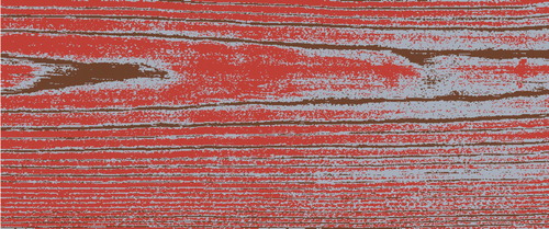
Smeland et al. (2016) found that the wood segmentation algorithm they developed worked best using the second principal component from PCA and suggested that thresholds be positioned at the 25th and 65th percentile in the scores histogram. For our dataset however, we found that, when performing PCA on the absorbance data, the first principal component worked better than the second and that the percentile thresholds needed to be tweaked manually for each sample in order to adequately approximate the early- and latewood distribution observed by studying the samples visually. An example of a generated image segmentation mask can be seen in Figure 4. In the figure, red color indicates earlywood, brown color indicates latewood, the intermediary region between the two classes which was not considered as either early- or latewood is shown in gray. Since our samples were kept stationary during the time series acquisition and only negligible contraction of the samples was found to take place during the drying process, the segmentation was performed only once per sample and then applied to all images within the time series. The segmentation was performed using the last image of each series, i.e. the image corresponding to the driest sample state.

Figure 4. Spatial early-/latewood segmentation of one of the samples in the study (sample S7). Brown color indicates pixels classified as latewood and red color indicates pixels classified as earlywood. Gray color indicates intermediate wood which was not treated as either early- or latewood.

3.2. PLS regression modeling

The grid search over spectral preprocessing techniques indicated that a combination of extended multiplicative scatter correction followed by first order Savitzky–Golay derivation yielded the lowest cross-validated prediction error. During EMSC the basic EMSC model (Afseth and Kohler 2012) was used, which entails a model containing an intercept term, slope term, linear term and a quadratic term. The average spectrum from the training dataset was used as a reference spectrum in the EMSC correction. The Savitzky–Golay derivation was carried out with a window size of seven and a polynomial degree of one.

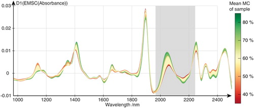
The best performing variable selection was identified using the moving window algorithm. Moving window selection is when a window iteratively traverses the entire spectra and a model is calibrated and cross-validated at each possible location using only the wavelengths within the window for each location. The window width and location found to result in the lowest cross-validated error is then used in the final model. In our experiment, the best region found by the algorithm consisted in 52 wavelengths between 1966 and 2244 nm. Figure 5 shows the average spectrum of every hyperspectral image in the dataset after preprocessing along the region identified during wavelength selection.

Figure 5. Mean absorbance spectrum of every time series image in the collected dataset preprocessed with basic EMSC followed by first order Savitzky-Golay derivation. Gray region indicates wavelength region identified by the moving window feature selection algorithm. All spectra in the figure are colored according to the average of moisture content of the sample they originate from.

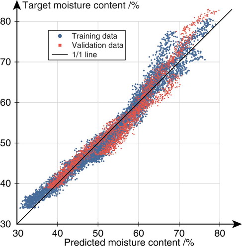
Using the combination of identified preprocessing and wavelength selection, the lowest RMSE_cv (and first local minima) after 10-fold cross-validation was obtained using nine PLS components, which was subsequently used when calibrating the final PLS model. Figure 6 shows a regression plot of PLS-modeled vs. average measured moisture content of each image in the eight time series sequences. Blue dots indicate data originating from any of the six training time series, red squares indicate data from the two validation time series. The model’s root-mean-squared-error, RMSE, on the training data was 2.1%, with a coefficient of determination, R², of 0.98. Applying the model to the validation data resulted in a RMSE of 2.7% and a R² of 0.97. For most samples in the study, the discrepancy between modeled MC and sample-average MC was larger during the first few hours of drying compared to the rest of the drying sequence.

Figure 6. Regression plot of PLS modeled vs. measured mean moisture content for every image of the dataset. Blue dots represent images belonging to the training data, red squares represent images belonging to the validation data.

3.3. PLS modeled spatial distribution & temporal development of moisture content

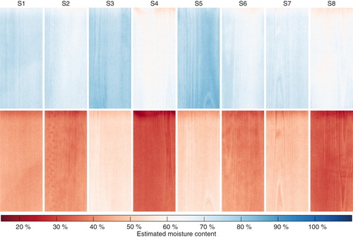
 Figure 7 shows chemical maps of the PLS-estimated spatial distribution of moisture content for every sample in the study obtained by applying the PLS model to the full resolution hyperspectral data. The upper row depicts the samples at the start of their time series, i.e. after 100 min of drying. The lower row depicts the same samples at the end of their time series, i.e. after 21.5 h of drying. Some samples, such as S4, S6, S7 and S8, can be seen in the figure to have a locally higher moisture content at the top of the sample, indicating a slower rate of drying at the top. A possible explanation for this could be that the Spectralon white reference plate, which in our experimental setup is located at the top edge of the sample, is hindering drying to freely take place at the top of the sample.

Figure 7. Spatial distribution of PLS-estimated moisture content for every sample in the study. Upper row depicts the samples at the initial stages of drying, lower row depicts the same samples approximately 20 h of drying later.

 Figure 8 shows the average PLS-estimated early- and latewood moisture content for every image in the dataset displayed as eight individual time series/drying curves. These curves were obtained by applying the developed early-/latewood segmentation masks of each sample onto the modeled spatial distribution of moisture content for every time step in the series. The moisture content estimates for all early- and latewood pixels were then separately averaged to form two drying curves per sample; one containing the estimated drying curve for latewood and the other for earlywood.

Figure 8. Temporal development of predicted moisture content of all samples (S1-S8). In each subplot the orange lines indicate the average modeled moisture content in all earlywood pixels of a sample, blue lines indicate the average moisture content in the latewood pixels of a sample.

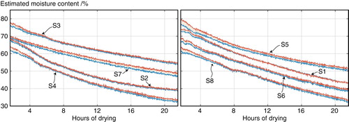
During the first few hours of drying the estimated moisture content of the earlywood was noticeably higher than the latewood estimates for all samples. Averaged across all samples the estimated moisture content was 1.7% higher in the earlywood than the latewood at the beginning of the time series and decreased over time down to a 0.8% difference at the end of the drying process. The samples with the lowest estimated moisture difference between early- and latewood, S2, S1 and S3, all have a fine grained early- and latewood structure with densely packed growth regions as can be seen in Figure 7. It is also interesting to note that the sample with the greatest radial annual ring distance of the sample set, S5, also had the largest estimated moisture differential between early- and latewood (2.9% during the initial stages of drying).

4. Discussion & conclusions

Our developed PLS model, calibrated on six time series consisting of 7176 hyperspectral images in total, proved capable of estimating the sample-average moisture content of thermally modified pine at different points in time during drying with a high degree of accuracy. Extended multiplicative scatter correction combined with first order derivation proved useful in relieving light scatter effects from the spectra and enhancing the correlation between spectra and moisture content. The wavelength region 1966–2244 nm was found to hold strong predictive capacity over the moisture content of the pine. This region includes several wavelengths which are known to cause absorption in free water at room temperature, although it slightly misses the absorption peak which occurs around 1930–1950 nm (Curcio and Petty 1951). Fujimoto et al. (2008) found 1980nm to be a region representative of water absorption in larch wood, which is included in our identified region. Our model produced the best results at nine principal components, which is rather high. Kobori et al. (2013) found six PLS components to be optimal for estimating MC in unmodified pine using vis-NIR hyperspectral spectral data—thus, both experiments indicate that a surprisingly high number of latent variables is beneficial when estimating the moisture content of pine using PLS regardless of wood treatment.

By superimposing a segmentation mask onto the PLS-estimated spatially and temporally resolved distributions of moisture content, our presented method allows separate estimates to be obtained of the MC of early- and latewood regions within a board during drying. However, as is often the case with studies such as this one—were a model is trained using a measured sample-average response value and later used to estimate the spatial distribution of the response throughout the sample—a major limitation is that the chemical maps generated by the regression model cannot easily be validated; since the true pixel-by-pixel distribution of moisture is unknown to us. We therefore cannot conclude that the spatial predictions are accurate, only that the spatial estimates appear realistic upon visual inspection and that the PLS model is capable of estimating the average moisture content of a thermally modified pine sample based on the average spectra of the sample. Further studies should therefore investigate the possibility of training a regression model with hyperspectral input data together with spatially resolved response values—obtained for instance by using magnetic resonance imaging on the same samples as are scanned with a hyperspectral camera.

Despite the successfulness of using surface reflected visible and near-infrared radiation to model the moisture content of wood samples, demonstrated in this study for thermally modified pine as well as in Kobori et al. (2013) for unmodified pine, it is important to note that such models rest on the assumption that the moisture content is consistent throughout the thickness of the sample. This assumption is of course never entirely valid, and it likely increases in invalidity when thicker wood samples are used with a more inhomogeneous internal annual ring structure. To circumvent this issue entirely remote sensing technologies with a greater penetration depth, such as MRI, are necessary. To lessen the effects of this limitation in our own experimental setup, thinner samples could have been used in our experiment—such that there is less room for unobserved radial moisture variations in the sample. In some preliminary experiments we conducted prior to the experiment presented here however, we monitored thinner samples with hyperspectral imaging and found that although it certainly seems possible to estimate the moisture content of such samples, the drying dynamics of thin samples (∼2-3 mm thickness) appears substantially different from that of thicker boards (∼2 cm thickness). When using thin samples the moisture evaporated rapidly around the edges of the sample when exposed to the warm halogen light of the experimental setup. Our motivation for choosing larger samples in this experiment is that we wanted a slower, more controlled, drying process.

Lastly it should be mentioned that we in our paper have chosen to calibrate our model using a moisture content which expresses the weight of the moisture in the wood in relation to the wood’s dry matter according to Equation 1.

In Equation 1 $w_{\mathrm{w}\mathrm{e}\mathrm{t}\mathrm{w}\mathrm{o}\mathrm{o}\mathrm{d}}$ is the weight of the drying sample and $w_{\mathrm{d}\mathrm{r}\mathrm{y}\mathrm{w}\mathrm{e}\mathrm{i}\mathrm{g}\mathrm{h}\mathrm{t}}$ is the weight of the sample in its dry state. This moisture content formulation is commonly used in wood science and calibrating models to approximate this value from hyperspectral data has previously been proven viable (Kobori et al. 2013). However, an alternative approach would be to use the mass percentage of the water when calibrating the model, i.e. the mass of the constituent of interest (water) divided by the total mass of the object multiplied by 100:(4) $\mathrm{M}\mathrm{a}\mathrm{s}\mathrm{s}\mathrm{P}\mathrm{e}\mathrm{r}\mathrm{c}\mathrm{e}\mathrm{n}{\mathrm{t}}_{\mathrm{w}\mathrm{a}\mathrm{t}\mathrm{e}\mathrm{r}}=\frac{w_{\mathrm{w}\mathrm{e}\mathrm{t}\mathrm{w}\mathrm{o}\mathrm{o}\mathrm{d}}-w_{\mathrm{d}\mathrm{r}\mathrm{y}\mathrm{w}\mathrm{e}\mathrm{i}\mathrm{g}\mathrm{h}\mathrm{t}}}{w_{\mathrm{w}\mathrm{e}\mathrm{t}\mathrm{w}\mathrm{o}\mathrm{o}\mathrm{d}}}\cdot 100\left(\text{\%}\right)$(4)

Given a $\mathrm{M}\mathrm{a}\mathrm{s}\mathrm{s}\mathrm{P}\mathrm{e}\mathrm{r}\mathrm{c}\mathrm{e}\mathrm{n}{\mathrm{t}}_{\mathrm{w}\mathrm{a}\mathrm{t}\mathrm{e}\mathrm{r}}$ value, the conventional MC, expressed in relation to the wood’s dry matter, can then be obtained using the conversion:(5) $\mathrm{M}\mathrm{C}=\frac{\mathrm{M}\mathrm{a}\mathrm{s}\mathrm{s}\mathrm{P}\mathrm{e}\mathrm{r}\mathrm{c}\mathrm{e}\mathrm{n}{\mathrm{t}}_{\mathrm{w}\mathrm{a}\mathrm{t}\mathrm{e}\mathrm{r}}}{1-\left(\mathrm{M}\mathrm{a}\mathrm{s}\mathrm{s}\mathrm{P}\mathrm{e}\mathrm{r}\mathrm{c}\mathrm{e}\mathrm{n}{\mathrm{t}}_{\mathrm{w}\mathrm{a}\mathrm{t}\mathrm{e}\mathrm{r}}/100\right)}\left(\text{\%}\right)$(5)

Since absorbance spectra are related to the mass of an absorbing species in relation to the mass of the sample as a whole, it should in theory be advantageous to calibrate a model using a target variable produced by Equation 4 and then converting the model’s output to a conventional moisture content using Equation 5, as opposed to calibrating the model on the values produced by Equation 1. Employing this strategy may help to resolve the nonlinearity present in our results, observed in Figure 6 predominantly at low moisture contents. The primary culprit of the deviations observed in Figure 6 may be our choice of target variable (Equation 1), the use of which is not as theoretically well-grounded in the domain of spectroscopic modeling as the use of Equation 4. Future studies should, therefore, investigate if the “detour” of calibrating a model on the values produced using Equation 4 and then converting the model’s output using Equation 5 is superior to calibrating directly on the conventional moisture content produced by the Equation 1.

Disclosure statement

No potential conflict of interest was reported by the author(s).

References

- Afseth, N. K. and Kohler, A. (2012) Extended multiplicative signal correction in vibrational spectroscopy, a tutorial. Chemometrics and Intelligent Laboratory Systems, 117, 92–99.
- Barnes, R., Dhanoa, M. and Lister, S. J. (1989) Standard normal variate transformation and de-trending of near-infrared diffuse reflectance spectra. Applied Spectroscopy, 43(5), 772–777.
- Björck, Å and Indahl, U. G. (2017) Fast and stable partial least squares modelling: A benchmark study with theoretical comments. Journal of Chemometrics, 31(8), e2898.
- Bohumil, K. (1992) Skandinaviske normer for testing av små feilfrie prøver av heltre (Ås, Norway: Skogforsk. Norwegian Forest Research Institute).
- Brelid, P. L. (2013) Benchmarking and State of the Art for Modified Wood (Borås: SP Technical Research Institute of Sweden).
- Cirule, D., Meija-Feldmane, A., Kuka, E., Andersons, B., Kurnosova, N., Antons, A. and Tuherm, H. (2015) Spectral sensitivity of thermally modified and unmodified wood. BioResources, 11(1), 324–335.
- Curcio, J. A. and Petty, C. C. (1951) The near infrared absorption spectrum of liquid water. Journal of the Optical Society of America, 41(5), 302.
- Dunningham, E. and Sargent, R. (2015) Review of New and Emerging International Wood Modification Technologies (Melbourne: Forest & Wood Products Australia).
- Edward, C. P. (1957) How Wood Shrinks and Swells (Wisconsin: Forest Service, U.S. Department of Agriculture).
- Esteves, B. and Pereira, H. (2009) Wood modification by heat treatment: A review. BioResources, 4, 370–404.
- Fang, S., Zhu, M.-Q. and He, C.-H. (2009) Moving window as a variable selection method in potentiometric titration multivariate calibration and its application to the simultaneous determination of ions in Raschig synthesis mixtures. Journal of Chemometrics, 23(3), 117–123.
- Fujimoto, T., Kobori, H. and Tsuchikawa, S. (2012) Prediction of wood density independently of moisture conditions using near infrared spectroscopy. Journal of Near Infrared Spectroscopy, 20(3), 353–359.
- Fujimoto, T., Kurata, Y., Matsumoto, K. and Tsuchikawa, S. (2008) Application of near infrared spectroscopy for estimating wood mechanical properties of small clear and full length lumber specimens. Journal of Near Infrared Spectroscopy, 16(6), 529–537.
- Geladi, P. and MacDougall, D. M. H. (1985) Linearization and scatter-correction for near-infrared reflectance spectra of Meat. Applied Spectroscopy, 39(3), 491–500.
- Hameury, S. and Sterley, M. (2006) Magnetic resonance imaging of moisture distribution in Pinus sylvestris L. exposed to daily indoor relative humidity fluctuations. Wood Material Science and Engineering, 1(3-4), 116–126.
- Hill, C. A. S. (2006) Wood Modification (Chichester: Wiley).
- Javed, M. A., Kekkonen, P. M., Ahola, S. and Telkki, V.-V. (2015) Magnetic resonance imaging study of water absorption in thermally modified pine wood. Holzforschung, 69(7), 899–907.
- Jiang, J.-H., Berry, R. J., Siesler, H. W. and Ozaki, Y. (2002) Wavelength interval selection in multicomponent spectral analysis by moving window partial least-squares regression with applications to mid-infrared and near-infrared spectroscopic data. Analytical Chemistry, 74(14), 3555–3565.
- Kekkonen, P. M., Ylisassi, A. and Telkki, V.-V. (2014) Absorption of water in thermally modified pine wood as studied by nuclear magnetic resonance. The Journal of Physical Chemistry C, 118(4), 2146–2153.
- Kobori, H., Gorretta, N., Rabatel, G., Bellon-Maurel, V., Chaix, G., Roger, J.-M. and Tsuchikawa, S. (2013) Applicability of Vis-NIR hyperspectral imaging for monitoring wood moisture content (MC). Holzforschung, 67(3), 307–314.
- Martens, H. and Stark, E. (1991) Extended multiplicative signal correction and spectral interference subtraction: New preprocessing methods for near infrared spectroscopy. Journal of Pharmaceutical and Biomedical Analysis, 9(8), 625–635.
- MATLAB (2019) MATLAB, Version 9.6.0 (R2019a) (Natick, Massachusetts: The MathWorks Inc).
- Myronycheva, O., Sidorova, E., Hagman, O., Sehlstedt-Persson, M., Karlsson, O. and Sandberg, D. (2018) Hyperspectral imaging surface analysis for dried and thermally modified wood: An exploratory study. Journal of Spectroscopy, 2018, 1–10.
- Nørgaard, L. S. A., Wagner, J., Nielsen, J., Munck, L. and Engelsen, S. (2000) Interval partial least-squares regression (iPLS): A comparative chemometric study with an example from near-infrared spectroscopy. Applied Spectroscopy, 54(3), 413–419.
- Rinnan, Å, Berg, F. v. d. and Engelsen, S. B. (2009) Review of the most common pre-processing techniques for near-infrared spectra. TrAC Trends in Analytical Chemistry, 28(10), 1201–1222.
- Sandak, A., Sandak, J. and Negri, M. (2010) Relationship between near-infrared (NIR) spectra and the geographical provenance of timber. Wood Science and Technology, 45(1), 35–48.
- Sandak, J., Sandak, A., Pauliny, D., Krasnoshlyk, V. and Hagman, O. (2013) Near infrared spectroscopy as a tool for estimation of mechanical stresses in wood. Advanced Materials Research, 778, 448–453.
- Sandberg, D. and Kutnar, A. (2016) Thermally modified timber: recent developments in Europe and North America. Wood and Fiber Science, 48, 28–39.
- Savitzky, A. and Golay, M. J. E. (1964) Smoothing and differentiation of data by simplified least squares procedures. Analytical Chemistry, 36(8), 1627–1639.
- Schweitzer, P. A. (1999) Atmospheric Degradation and Corrosion Control (New York: M. Dekker), p. 197.
- Smeland, K. A., Liland, K. H., Sandak, J., Sandak, A., Gobakken, L. R., Thiis, T. K. and Burud, I. (2016) Near infrared hyperspectral imaging in transmission mode: Assessing the weathering of thin wood samples. Journal of Near Infrared Spectroscopy, 24(6), 595–604.
- Stefansson, P., Fortuna, J., Rahmati, H., Burud, I., Konevskikha, T. and Martens, H. (2019a) Hyperspectral time series analysis: Hyperspectral image data streams interpreted by modeling known and unknown variations. In Jose Manuel Amigo (ed.) Hyperspectral Imaging, Volume 32, 1st ed. (Copenhagen: Elsevier), pp. 305–331.
- Stefansson, P., Indahl, U. G., Liland, K. H. and Burud, I. (2019b) Orders of magnitude speed increase in partial least squares feature selection with new simple indexing technique for very tall datasets. Journal of Chemometrics, 33(11), 1–9.
- Watanabe, K., Mansfield, S. D. and Avramidis, S. (2011) Application of near-infrared spectroscopy for moisture-based sorting of green hem-fir timber. Journal of Wood Science, 57(4), 288–294.