Stochastic optimisation of long-term block cave scheduling with hang-up and grade uncertainty

Abstract

Mass mining methods provide alternatives in developing deeper and lower-grade mineral deposits. Consequently, block cave mining has been increasingly popular mass mining method, especially for large copper deposits currently being mined by open pit methods. This study adopts similar concepts as in stochastic open pit production planning to the planning of block cave mines, to evaluate their effectiveness in a different approach to mass mining. The main contribution of this study is the incorporation of the uncertainty of delays from hang-ups and grades directly into the production scheduling process of a cave mining operation. Hang-up uncertainty relates to the uncertainty linked to the occurrence of ore that clogs the production draw points. This clogging causes time delays in the production cycle leading to tonnage losses and additional costs. Grade uncertainty is incorporated by means of stochastic orebody simulations. Both uncertainty sources are directly linked to the extraction decisions and influence the optimized schedules. The proposed stochastic integer programming model is applied to the optimization of the long-term schedule of a large-scale, low-grade copper deposit by taking into account hang-up delays in block caving. The results of the optimization maximizing net present value clearly show the capability of the formulation to mitigate the effects of both grade and hang-up uncertainty.

Keywords:

• Mine production scheduling
• block caving
• stochastic integer programming
• hang-up delays
• stochastic schedule optimisation
• technical risk management

1. Introduction

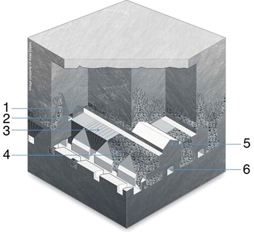
Block caving is a nonselective underground mining method that extracts ore from the bottom of the orebody to the top. This is achieved by developing production levels below the orebody before the extraction is started as shown in Figure 1. Once all development is completed, the orebody is undercut by blasting a layer of ore (1 and 2 in Figure 1). After the undercutting, the rock mass above starts to cave under its own weight and in situ rock stresses. The broken ore is extracted by load-haul-dump (LHD) machines from the draw points located in the production level (4 and 6 in Figure 1). The planning of block cave mines focuses on the sequence of extraction from these draw points. The plan has to determine how much is to be extracted from which draw points for each period. The basic extraction unit is called a slice and represents the vertical discretisation of the column of ore above a draw point. The schedule also has to decide when new draw points are opened. A major surge in block caving projects for base metal production is currently observed all over the world with various projects starting up or being near the end of the feasibility process, such as Oyu Tolgoi (Mongolia), Resolution (Arizona, US), Chuiquicamata (Chile), DMLZ Grasberg (Indonesia), etc. [1].

Figure 1. Illustration of a block cave mine (©Atlas Copco): 1. blast holes for the undercut, 2. undercut level, 3. blast holes for the draw bell construction, 4. draw point, 5. major apex (the in situ rock that defines the draw points) and 6. production drift.

Chanda [2] proposes a short-term schedule optimisation on a shift basis by a combination of a mixed integer programming (MIP) optimisation, which creates the schedule and a simulation model of the ore flow, which uses the earlier mentioned schedule as an input. Guest et al. [3] propose a linear programming formulation to optimise the long-term schedule of a block caving operation as a part of a draw control system. Rahal et al. [4] develop an MIP-model for the long-term optimisation of the shape of the draw profile. Pourrahimian et al. [5] consider a multi-step optimisation of an MIP model. The first step is an optimisation on clusters of draw points, the second step optimises for the draw points individually within the clusters, and finally a slice-based optimisation within each draw point is performed. Pourrahimian and Askari-Nasab [6] propose an MIP model where the best-height-of-draw (BHOD) follows directly from the optimisation on clusters of slices. The proposed model in this paper also determines the BHOD as a result of the optimisation. Khodayari and Pourrahimian [7] discuss most of the recent approaches to block cave scheduling using operations research methods. Diering et al. [8] present a deterministic approach called PCBC, which is the industry standard programme for block cave scheduling.

All the formulations above consider a single estimated orebody model. However, estimated orebodies smooth grades and give rise to unrealistic mine plans and unlikely revenue forecasts [9,10]. Malaki and Pourrahimian [11] and Vargas et al. [12] define the optimal footprint, the size and depth of the extraction level, of a cave mine under geological uncertainty. Dimitrakopoulos and Grieco [13] develop a probabilistic method for the definition of stopes in an underground mine incorporating geological uncertainty. Carpentier et al. [14] propose a stochastic integer program (SIP) for underground mine planning for a mining method that is a hybrid between cut-and-fill and long hole stoping. Their formulation includes geological (grade) uncertainty, while the access to and scheduling of underground ore zones are optimised. Montiel et al. [15] present the long-term simultaneous stochastic optimisation of a gold mining complex that includes both underground and open pit mines. Issues related to life-of-mine planning and the integration and management of geological risk (grades, material types, boundaries of geological zones) based on stochastic optimisation for open pit mines are discussed in several studies [16–18, and others]. Geological uncertainty is addressed through the geostatistical simulation framework [19–22] of the pertinent attributes of a mineral deposit.

The second source of uncertainty comes from the delays from hang-ups in draw points. A hang-up is defined as caved ore, which, due to its size (too fine or too coarse), obstructs the draw point and temporarily stops production from it. This production stoppage results in time delays, which in turn, cause tonnage losses and additional remediation costs. Rubio and Dunbar [23] and Rubio and Troncoso [24] consider hang-up frequency and impact uncertainty and show how it influences the maximum available production tonnage of a caving operation. Ngidi and Pretorius [25] also demonstrate the influence that hang-ups can have on a production system. However, the aforementioned authors do not integrate hang-up uncertainty directly into the schedule optimisation. They provide methods to quantify the influence of hang-ups without considering its direct effect on production schedule optimisation through which its influence can be mitigated.

The proposed method explicitly includes hang-up uncertainty in the optimisation model, where it can influence the extraction schedule to minimise the total delays. The influence that the delays from hang-ups can have is acknowledged by industry experts as one of the major issues that arise in current long-term plans. By integrating the delays directly in the optimisation process, the proposed model can mitigate their effect and produce more reliable long-term plans. The model proposed in this paper also considers the geological uncertainty of the metal grade. This has been proven to improve long-term scheduling results for open pit formulations in various instances [26–28]. The dilution process inherent in cave mining is modelled for each grade simulation via a simple mixing algorithm as presented in Laubscher [29]. Many other sources of uncertainty and delays for block caving, such as fragmentation, geomechanics, equipment failures, oversize for the equipment are acknowledged, but not considered in the proposed model.

The following sections first discuss the used optimisation model and specify all constraints. Second, the solution approach for the proposed model is explained. The last section discusses the case study. The discussion of the case study opens with an explanation of the used parameters for the optimisation, the modelling of the two types of uncertainty is detailed thereafter and finally the results of the optimisation are presented.

2. Method

2.1. Overview

The optimisation of the long-term block caving schedule under uncertainty is modelled as a SIP with recourse. This SIP with recourse was first applied to mine planning by Dimitrakopoulos and Ramazan [30]. Its success has been shown many times in the past for open pit planning [15,26–28,31,32]. The proposed model is the first application of a model of this kind to the scheduling of a block caving operation. The used recourse model allows for deviations from constraints, meaning that over- or underproduction is permitted. The optimisation model maximises the net-present-value (NPV) of the block caving operation, while it minimises time deviations caused by the hang-up uncertainty and grade deviations caused by the grade uncertainty.

2.2. Optimisation model

Tables 1–6 include the sets, variables and parameters used in the formulation (1)–(19). All variables are positive; $z_d^t$, $a_d^t$, and $y_{\mathit{id}}^t$ ∈ {0, 1} and $x_{\mathit{id}}^t\le 1$.

Table 1. Overview of the sets used for the sub- and superscripts in the formulation.

Sets
T	Set of the time periods in the life-of-mine
D	Set of the draw points
Id	Set of the slices per draw point
S	Set of the grade scenarios
H	Set of the hang-up scenarios
J	Set of the bottlenecks

Table 2. Overview of the decision variables.

Decision variables
$a_d^t$	Binary variable denoting the activity of draw point d in period t
$z_d^t$	Binary variable denoting the opening of draw points d by period t
$y_{\mathit{id}}^t$	Binary variable denoting the activity of slice i in draw point d by period t
$x_{\mathit{id}}^t$	Continuous variable denoting the extraction percentage of slice i in draw point d in period t

Table 3. Overview of the deviation variables.

Deviation variables
$TimeDe{v}_{d,+}^{\mathit{th}}$	Continuous variable denoting the time exceeding the limit in hang-up scenario h for draw point d in period t [in h]
$GradeDe{v}_{-}^{\mathit{ts}}$	Continuous variable denoting the shortcoming in the grade target at the mill for grade scenario s in period t [in g/t]
$MillTonDe{v}_{+}^t$	Continuous variable denoting the tonnage exceeding the target at the mill in period t [in t]
$MillTonDe{v}_{-}^t$	Continuous variable denoting the tonnage shortfall for the target at the mill in period t [in t]

Table 4. Overview of the economic parameters in the formulation.

Economic parameters
r	The financial discount rate [in %]
MetalPrice^t	The undiscounted metal price per ton Cu in period t [in $/t]
ProcessCost^t	The undiscounted processing cost per ton of ore in period t [in $/t]
MineCost^t	The undiscounted mining cost per ton of ore in period t [in $/t]
OpeningCost^t	The undiscounted opening cost per draw point in period t [in $/DP]
ActivityCost^t	The undiscounted cost of keeping a draw point active in period t [in $/year]
DelayCost^t	The undiscounted cost per hour lost due to a hang-up in period t [in $/h]

Table 5. Overview of the model parameters in the formulation.

Model parameters
g	The geological discount rate [in %]
$C_{\dots }^t$	The undiscounted penalty terms for the various deviations in period t
$Grad{e}_{\mathit{id}}^s$	The grade of slice i in draw point d for scenario s [in g/t]
Ton id	The tonnage of slice i in draw point d [in t]
Time id	The extraction time in hours of slice i in draw point d [in h]
$Dela{y}_{\mathit{id}}^h$	The delay in hours of a hang-up for slice i in draw point d for scenario h [in h]
P d′	The precedence set for draw point d’
P i′	The precedence set for slice i’
Adj(d′)	The set of adjacent draw points of draw point d’
$AbsDif{f}_{\mathit{Max}}^{td{d}^{\prime }}$	The maximum absolute extracted tonnage difference between adjacent draw points d and d’ in period t [in t]

Table 6. Overview of the operating parameters in the formulation.

Operating parameters
Rec	The metallurgical recovery at the mill [in %]
$A_{\mathit{Max}}^t$	The maximum number of active draw points in period t
$Z_{\mathit{Max}}^t$	The maximum number of draw points that can be opened in period t
$D{P}_{\mathit{Max}}^t$	The maximum extraction capacity of a draw point in period t [in t/year]
$D{P}_{\mathit{Min}}^t$	The minimum extraction requirement of a draw point in period t [in t/year]
$TimeD{p}_{d,Max}^t$	The maximum amount of time available for draw point d in period t [in h]
$BottleNec{k}_{j,Max}^t$	The capacity of bottleneck j in period t [units vary by type of bottleneck as explained below, mostly in t]
MillTonTarget^t	The tonnage target at the mill in period t [in t]
GradeTarget^t	The grade target at the mill in period t [in g/t]

The objective function in Equation (1) maximises the NPV and at the same time minimises deviations from targets. Three types of deviations are considered. First are the deviations from the mill tonnage target. Second, the grade deviation to control the influence of the grade uncertainty. Finally, the time deviation, the main contribution of this model, to control the influence of the delays from hang-ups. The penalty costs for the deviations (denoted by $C_{\dots }^t$ in Equation (1)) are discounted in terms of geological risk discounting (GRD), as introduced by Dimitrakopoulos and Ramazan [33]. GRD allows to control risk in meeting production targets; more specifically, it minimises deviations in early production years and defers risk (of not meeting production targets) to later periods when more information will become available. The objective function shows the value calculation on a block basis with a fixed recovery. This is a simplification required to keep the model linear such that it is solvable using commercially available optimisers. To make the notation shorter and simpler, it is assumed that $z_d^0=0$ for all draw points. The opening of draw points is modelled as an ‘opened-by’ variable as proposed by Caccetta and Hill [34] for the open-pit mining context. This formulation has been proved to be stronger than the more intuitive ‘opened-in’ formulation.

(1) $$\begin{array}{c}\mathit{Max}\frac{1}{S}\sum _{s=1}^S\sum _{t=1}^T\sum _{d=1}^D\sum _{i=1}^I\left[\frac{MetalPric{e}^t}{{\left(1+r\right)}^t}·Rec·Grad{e}_{\mathit{id}}^s·To{n}_{\mathit{id}}·x_{\mathit{id}}^t\right]\hfill \\ --\frac{1}{H}\sum _{h=1}^H\sum _{t=1}^T\sum _{d=1}^D\sum _{i=1}^I\left[\frac{DelayCos{t}^t}{{\left(1+r\right)}^t}·Dela{y}_{\mathit{id}}^h·x_{\mathit{id}}^t\right]\hfill \\ -\sum _{t=1}^T\sum _{d=1}^D\sum _{i=1}^I\left[\left(\frac{MineCos{t}^t}{{\left(1+r\right)}^t}+\frac{ProcessCos{t}^t}{{\left(1+r\right)}^t}\right)·To{n}_{\mathit{id}}^{}·x_{\mathit{id}}^t\right]\hfill \\ -\sum _{t=1}^T\sum _{d=1}^D\left[\frac{OpeningCos{t}^t}{{\left(1+r\right)}^t}·\left(z_d^t-z_d^{t-1}\right)+\frac{ActivityCos{t}^t}{{\left(1+r\right)}^t}·a_d^t\right]\hfill \\ -\sum _{t=1}^T\left[\frac{C_{millton+}^t}{{\left(1+g\right)}^t}·MillTonDe{v}_{+}^t+\frac{C_{millton-}^t}{{\left(1+g\right)}^t}·MillTonDe{v}_{-}^t\right]\hfill \\ -\frac{1}{H}\sum _{h=1}^H\sum _{t=1}^T\sum _{d=1}^D\left[\frac{C_{\mathit{time}}^t}{{\left(1+g\right)}^t}·TimeDe{v}_{d,+}^{\mathit{th}}\right]-\frac{1}{S}\sum _{s=1}^S\sum _{t=1}^T\left[\frac{C_{\mathit{grade}}^t}{{\left(1+g\right)}^t}·GradeDe{v}_{-}^{\mathit{ts}}\right]\hfill \end{array}$$(1)

Constraints (2) and (3) limit the number of active draw points from which material can be extracted, and the number of draw points that can be opened in each period.

(2) $$\sum _{d=1}^D{a}_d^t\le A_{\mathit{Max}}^t\forall t$$(2)

(3) $$\sum _{d=1}^D{z}_d^t\le Z_{\mathit{Max}}^t\forall t$$(3)

Constraints (4) govern the precedence sequence of opening new draw points. The precedence refers to which draw points have to be started before the next one can be started. This is similar to the slope constraints in open pit optimisation. However, in block caving, this is an operational constraint that is necessary to avoid isolated drawing from draw points to reduce dilution and improve recovery control, while in open pit mining it is a physical constraint. Constraints (5) ensure that the extraction of a slice can begin only if all the slices underlying it are extracted.

(4) $$z_d^t\le z_{d^{\prime }}^t\forall t,d\mathrm{and}\forall {\mathrm{d}}^{\prime }\in {\mathrm{P}}^{\mathrm{d}}$$(4)

(5) $$y_{\mathit{id}}^t\le \sum _{t^{\prime }=1}^t{x}_{\mathit{id}}^t\forall t,d,i\mathrm{and}\forall {\mathrm{i}}^{\prime }\in {\mathrm{P}}^{\mathrm{i}}$$(5)

A maximal extraction capacity per draw point per period is controlled by Constraints (6). This is required due to limitations of the LHDs and the draw rate.

(6) $$\sum _{i=1}^I\left(To{n}_{\mathit{id}}·x_{\mathit{id}}^t\right)\le D{P}_{\mathit{Max}}^t·a_d^t\forall t,d$$(6)

Constraints (7) and (8) avoid that mining from draw points is started and stopped at will, as this is not realistic due to geomechanical issues. Indeed, once mining from a draw point is stopped, it is very difficult (if not impossible) to re-start production. The minimal extraction requirement imposed by Constraints (9) ensure that a certain tonnage is extracted from each active draw point. Combined, Constraints (7)–(9) ensure the continuous extraction from active draw points.

(7) $$a_d^t-a_d^{t-1}\le z_d^t-z_d^{t-1}\forall t\ge 2,\forall d$$(7)

(8) $$a_d^1=z_d^1\forall d$$(8)

(9) $$a_d^t·D{P}_{\mathit{Min}}^t\le \sum _{i=1}^I\left(To{n}_{\mathit{id}}·x_{\mathit{id}}^t\right)\forall t,d$$(9)

Constraints (10) guarantee that the difference in the quantity of extracted ore between adjacent draw points is below a given threshold. These constraints are required to keep a relatively smooth cave front, which avoids stress-induced stability issues and reduces dilution.

(10) $$\sum _{i=1}^I\left(To{n}_{\mathit{id}}·x_{\mathit{id}}^t\right)-\sum _{i=1}^I\left(To{n}_{i{d}^{\prime }}·x_{i{d}^{\prime }}^t\right)\le AbsDif{f}_{\mathit{Max}}^{td{d}^{\prime }}\forall t,d\mathrm{and}\forall {\mathrm{d}}^{\prime }\in \mathrm{Adj}({\mathrm{d}}^{\prime })$$(10)

The above constraints are typically used in a block cave scheduling model; the only ‘unconventional’ constraints are the Constraints (11), which are added to govern the influence of delays caused by hang-ups. These constraints are modelled with one deviation allowing for overproduction, or better overtime in this case. Deviations are penalised in the objective function to reduce overtime. This leads to changes in extraction sequence and schedule through the $x_{\mathit{id}}^t$-variable in Constraints (11).

(11) $$\sum _{i=1}^I\left(Tim{e}_{\mathit{id}}+Dela{y}_{\mathit{id}}^h\right)·x_{\mathit{id}}^t-TimeDe{v}_{d,+}^{\mathit{th}}\le TimeD{p}_{d,Max}^t\forall t,d,h$$(11)

Constraints (12) and (13) govern the proper functioning of the mill. Constraints (12) have two deviations, and thus aim to achieve the exact mill target, but allow for over- and underproduction. The grade constraints in Constraints (13) have only one deviation, allowing for underproduction. This ensures a certain head grade at the mill, but a higher grade is not penalised. GradeAvg ^ts in Constraints (13) is defined in Equation (14).

(12) $$\sum _{d=1}^D\sum _{i=1}^I\left(To{n}_{\mathit{id}}·x_{\mathit{id}}^t\right)+MillTonDe{v}_{-}^t-MillTonDe{v}_{+}^t=MillTonTarge{t}^t\forall t$$(12)

(13) $$GradeAv{g}^{\mathit{ts}}+GradeDe{v}_{-}^{\mathit{ts}}\ge GradeTarge{t}^t\forall t,s$$(13)

(14) $$GradeAv{g}^{\mathit{ts}}=\frac{{\sum }_{d=1}^D{\sum }_{i=1}^I\left(Grad{e}_{\mathit{id}}^s·To{n}_{\mathit{id}}·x_{\mathit{id}}^t\right)}{{\sum }_{d=1}^D{\sum }_{i=1}^I\left(To{n}_{\mathit{id}}·x_{\mathit{id}}^t\right)}$$(14)

Constraints (15) are the bottleneck constraints and are written in a general form to represent multiple bottlenecks in the system. These constraints assume that all extracted tonnages pass through the bottleneck. Three bottlenecks are accounted for the set J: first, the underground sizers that do a size reduction of the ore after it is extracted by the LHDs from the draw points; second, the underground conveyors that transport ore in the underground workings from the sizers to the surface transportation conveyors; and finally, the conveyors that transport ore from the underground to the surface.

(15) $$\sum _{d=1}^D\sum _{i=1}^I\left(To{n}_{\mathit{id}}·x_{\mathit{id}}^t\right)\le BottleNec{k}_{j,Max}^t\forall t,j$$(15)

Constraints (16) ensure that every draw point can only be started once but does not have to be started. This is the typical reserve constraint of resource extraction optimisation.

(16) $$z_d^{t-1}\le z_d^t\forall t,d$$(16)

Constraints (17) link the extraction and activity variables, meaning: ‘Mining from a draw point forces it to be active’. A note on this linkage constraint is that the opposite (‘You cannot mine from an inactive draw point’.) is enforced by the combination of Constraints (6) and (9).

(17) $$\frac{{\sum }_{i=1}^I{x}_{\mathit{id}}^t}{I}\le a_d^t\forall t,d$$(17)

Constraints (18) link the starting of the slice in a draw point to the extraction percentages from that slice, meaning: ‘Extracting from a slice is only possible if that slice is started’. These constraints also ensure that no more than 100% can be extracted from

(18) $$\sum _{t^{\prime }=1}^t{x}_{\mathit{id}}^{t^{\prime }}\le y_{\mathit{id}}^t\forall t,d,i$$(18)

The linkage between the start and the activity of a slice keeps a slice active once it is activated and is given by Constraints (19). This allows extraction from a slice over multiple periods.

(19) $$y_{\mathit{id}}^{t-1}\le y_{\mathit{id}}^t\forall t\ge 2,\forall d,i$$(19)

3. Solution approach

The block caving SIP on a slice basis (1)–(19) introduced in the previous section is very difficult to solve due to the various linking constraints (17)–(19), precedence constraints (4) and (5), and especially because of the adjacent draw point constraints (10). It is solved with CPLEX in a C++ environment. Initial efforts to solve the whole optimisation at once for all periods without any reduction of the number of variables or any simplifications were unsuccessful. Even after 24 h, no solution for the linear relaxation was found.

Therefore, some variable reduction techniques and a heuristic are implemented. The first effort to reduce the solution time was to use the earliest start algorithms as introduced by Topal [35], which allows reducing the size of the problem by fixing 35% of the variables for the case study considered in this paper. The earliest start algorithm fixes variables based on implied bounds from Constraints (2), (3) and (6). Even after this variable reduction, the solution time was still very long and further measures to reduce the computational burden were taken. Specifically, a sliding time window heuristic (STWH) [30,36,37] was used. The STWH is based on a sequential solution of each period with binary variables while all following periods are relaxed. Once a solution for this period is found, the corresponding variables are fixed and the time window with binary variables is advanced. In more detail:

1. A time window of size |τ| is chosen. This window starts a period t. 


2. In this time window, all variables and constraints are added and defined in their regular form as described in the formulation above.

3. The variables in all other periods t ∉ τ are relaxed to be continuous. In some cases, the constraints are also relaxed by a Langrangian relaxation, but this is optional. Usually all constraints are added in full for all periods.

4. This is solved as a whole with the variables of periods t ∈ τ as binary and all others relaxed. The solution for the binary variables in period t is retained.

5. The window of size |τ| is moved one forward to start at t + 1 and all variables of period t are fixed to their solution from the previous optimisation.

6. This is repeated until a solution is found for all time periods t ∈ T.

Cullenbine et al. [36] apply this to open pit scheduling and show that a solution achieved in this manner is not far from an optimal solution even when using, |τ| = 1 and relaxing the constraints via Langrangian relaxation in all periods t ∉ τ. Lamghari and Dimitrakopoulos [37] also apply STWH with |τ| = 1, but the constraints are not relaxed in the other periods; the variables are only relaxed to be continuous. They also show good results. The same approach with |τ| = 1 and a relaxation of the variables in the other periods is taken herein. The constraints for all periods are always added in full. An advantage of the formulation, as presented above relating to the STWH, is that the x-variables and the extraction decisions from the slices are continuous and are thus optimised every time for the whole life-of-mine after the other binary variables have been fixed. The STWH also allows to revisit the earliest start algorithm for each period that has been solved based on the decisions that are made.

4. Case study

The first part of this section gives a brief overview of the size and scope of the case study and discusses some of the used parameters. The second part details how the two sources of uncertainty are modelled. The third and final part demonstrates the results of the optimisation.

4.1. Case study parameters

The proposed formulation is applied to a massive, homogeneous copper deposit in its prefeasibility stage. The goal of the optimisation is to assess the financial viability of a block caving project in the long-term future while incorporating grade and hang-up uncertainty. The geotechnical and geomechanical requirements for a caving project have been assessed by a professional consulting company and the deposit has been found favourable for caving in their report. The block size distribution, caveability and dilution are all in line with what has been considered to be viable for block caving. The design parameters (Table 7), footprint design and grid lay-out are provided by the engineering team of the mine site. The only modification by the authors is a size reduction of the footprint to keep the problem solvable with the chosen commercial solver. Consequently, the number of active draw points and the production profile are also scaled down from their original values.

Table 7. Overview of some parameter values for the optimisation.

Design parameters
Number of draw points [D]	408	Start draw rate	0.1 $\frac{t}{m^{2}d}$
Max new DP (a) [$Z_{\mathit{Max}}^t$]	100	Max draw rate	0.6 $\frac{t}{m^{2}d}$
Max active DP (a) [$A_{\mathit{Max}}^t$]	400	Slice height	16 m
Max production DP (a) [$D{P}_{\mathit{Max}}^t$]	42,120 t	Slice weight [Ton id ]	6755 t
Daily production	35,000 t	Rock density	2.5 $\frac{t}{m^3}$
Life-of-mine	12 years	Financial discount [r]	7%
Ramp-up	6 years	Geological discount [g]	15%

Notes: Annual quantities are denoted by (a). The daily production is for the whole mine after ramp-up. The related parameters from the model are added between the square brackets.

Table 7 shows some of the parameter values for the constraints that are used in the optimisation. The maximum draw rate is the maximum one allowed after the ramp- up is completed. A lower draw rate in certain draw points is permitted. The reported daily production leads to 12 Mt per year for the mill, when some spare flexibility is left for unexpected and unincorporated delays. With these parameters, the life-of-mine is 12 years, allowing for a full extraction of the orebody if the optimizer indicates that this is the optimal solution. The slice weight is based on its rock density and its surface area, as defined by a parallelogram with sides of 13 and 15 m and an acute angle of 60°. Table 7 does not show any information on the used cost and price data. This information was also provided by the mining company, but cannot be shared due to confidentiality reasons.

The considered precedence relation between the draw points is demonstrated in Figure 2. It is defined for a mining front in a wide V-shape. To be more specific, the draw points below the red lines have no predecessors and these can be readily started in the first period. Draw points above the red lines and below the blue lines can only be started if extraction of the draw points below the red lines has started. Similarly, the draw points above the red line and below the blue lines are the predecessors of the draw points below the green line and above the rightmost blue line (only the 5 draw points on the right). Predecessors for the whole footprint are defined in a similar fashion following the demonstrated V-shaped advancing front.

Figure 2. The precedence relations for the first draw points in plan view.

Notes: The coloured lines define the precedence relation. The arrow indicates the direction of mining. North is pointed straight up.

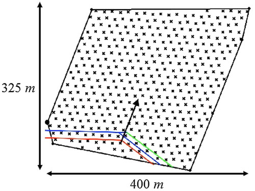
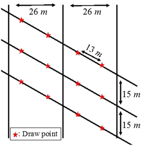
Figure 2 also shows the shape of the footprint, which is located approximately 500 m below the surface. The width of the footprint is 400 m and the length 325 m, leading to a surface area of ±80,000 m ² . This footprint contains a total of 408 draw points in a single panel with an El-Teniente grid lay-out. The spacing of the production drifts oriented to the north-east is 26 m and the spacing of the cross-headings that contain the draw points is 15 m. A detailed view of the El-Teniente grid is shown in Figure 3.

Figure 3. El-Teniente grid (26 m × 15 m).

Figure 4 shows in detail how the slices are defined in the column of ore above each draw point. These slices are used as the discretization unit of the orebody and all relevant parameters, such as time, tonnage, grades and hang-ups, are modelled on a slice basis. The total column is modelled up to a height of 512 m, which is approximately the distance to the surface. It is important to remark that the BHOD is not predefined, although it is limited to 512 m.

Figure 4. Definition of the slices in the column above an underlaid draw point.

4.2. Modelling of the uncertainty

The stochastic orebody simulations are generated by direct block simulation [16,38]. Fifteen orebody simulations are used for the optimisation and an additional fifteen different simulations are used for the generation of the risk profiles. Using different simulations for both the risk assessment and the optimisation provides a better representation of the risk resilience of the schedule.

The hang-up uncertainty is modelled as a distribution based on the tonnage between events (TBE), as in Rubio and Troncoso [24]. This varies with the slice location according to the possible height of the column of broken ore above that slice. The higher this column, the higher the vertical stress is and thus the higher the fragmentation and the lower the hang- up frequency are (or the higher the TBE), as presented by Gonzalez Iturriaga [39]. The expected time loss per hang-up is 1 h and 30 min, which is based on the performance of secondary breakage units provided by the engineering team of the mining company. The base case expected TBE for this operation is 1400 t of ore drawn per draw point. The base case refers to material right above the production level at the start of caving. Once caving is initiated, the column of fractured rock increases, and, based on the logic described above, the expected TBE increases too. This increase stops once the column of fractured ore reaches the surface at±500 m. From there on, it decreases, as does the expected TBE. The range of the expected TBE is modelled as a Gaussian distribution. One standard deviation up or down represents plus or minus 15% on the expected TBE. This information is provided as expert knowledge from the engineering team of the mining company. Kenzap and Kazakidis [40] show that this is often the best available information for a mining operation and can be used in preliminary assessments of a project’s financial viability. Five hang-up simulations are used for the optimisation, as this proved to be sufficient to cover the variability of the hang-ups. Fifteen different simulations are used for the risk assessment. It is important to stress that these simulations are a fixed input to the model and are not influenced by extraction decisions made during the optimisation.

4.3. Results of the optimisation

The case study focuses on four different cases to demonstrate the influence of both sources of uncertainty. In the rest of the paper, the bolded names in the list below will be used to indicate which of these cases is being addressed. The presented case study is solved with CPLEX 12.6.1 in a C++ environment on a computer with two Intel Xeon CPU E5-2697 v3 @ 2.60 GHz processors and 128 GB RAM.

1. The Conventional approach: assumes no delays and uses one single estimated ore-body model. This case is always represented in red in all figures below. This is a deterministic case and mimics the traditional optimizers discussed in the literature in Section 1.

2. The Stochastic HU approach: incorporates five delay scenarios into the optimisation and uses one single estimated orebody model. This case is always represented in green in all figures below.

3. The Stochastic G approach: assumes no delays and incorporates fifteen grade simulations into the optimisation. This case is always represented in orange in all figures below.

4. The Stochastic HU-G approach: incorporates five delay scenarios and fifteen grade simulations into the optimisation. This case is always represented in blue in all figures below.

The risk analyses are done by running the different scenarios of delays and grades through the optimised schedules of each of the four cases. This is then summarised by the tenth (P10), fiftieth (P50) and ninetieth (P90) percentiles. The P10 represents the low end of the distribution, being the best case for the delay scenarios and the worst case for the grade scenarios. The P90 represents the high end of the distribution, being the worst case for the delay scenarios and the best case for the grade scenarios. The P90 is always above the P50, the P10 is below the P50. All presented risk analyses include grade and/or hang-up uncertainty based on fifteen grade and fifteen hang-up scenarios not used in the optimisation.

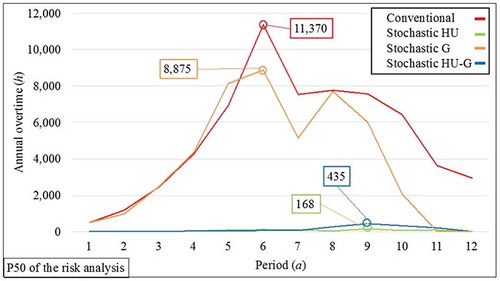
Figure 5 shows the P50 of the risk analysis for the overtime per period for the four different cases. The boxes highlight the maximum of the P50 of the overtime for each case. The overtime is calculated by summing up the time spent on slice extraction and the time incurred by delays within one period for all active draw points and subtracting from this the available time for extraction from these draw points. Therefore, the overtime is the additional time that is required to execute the proposed extraction schedule when delays from hang-ups occur, as would be the case during the operation of the mine. The delays used in this calculation are considered in 15 delay scenarios not used in the optimisation process, the P50 is the fiftieth percentile of all overtimes due to these scenarios. The first conclusion from this graph is the most important one from this work. The schedules that include hang-up uncertainty in the optimisation immensely outperform the schedules that do not. The annual overtime in the conventional and stochastic G cases is so high, right from the first periods, that these schedules, as well as their forecasted tonnages and NPV, are overly optimistic and unachievable. Using either of these schedules for calculating forecasts for a new block caving operation will drive the project into the ground as the operation will never achieve the forecasted production and thus NPV. The overtimes for the stochastic HU and HU-G cases are in stark contrast with the ones for the other two cases. The later are much lower and show the benefit of including the hang-up uncertainty and associated delays directly into the optimisation where they can influence the extraction schedule.

Figure 5. Comparison of the P50 of the risk analysis on the overtime for all four cases.

Note: The boxes highlight the highest overtime of the P50 for each case.

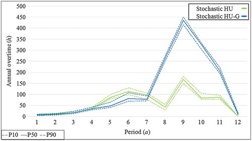
Figure 6 emphasises the risk profiles of the stochastic HU and HU-G schedules, which include hang-up uncertainty in the optimisation. It clearly shows that these schedules keep the annual overtime under control. Their overtime is never higher than 450 h, which is manageable with reactive planning on the short-term. It is noted that, as the material flow is not modelled explicitly in the simulation model and in order to provide a constraint to limit the dilution from intermixing of ore with waste at the caving interface front during the draw, a practical assumption was made to control the direct flow of ore to the draw point and to take into account the need for differential extraction cycle from draw points. The graph in Figure 6 also shows the effect of GRD: the overtime is larger in later periods because the penalty controlling it in the objective function is lower due to the discounting. This is desired because, as mining progresses, more information becomes available and the schedule can be altered based on the new information, effectively reducing the influence of delays in the later periods. The overtime decreases strongly in the last periods (11–12) because of the lower demand by the mill and, as such, most draw points have some overcapacity.

Figure 6. Comparison of the risk analysis on the overtime for the stochastic HU and stochastic HU-G cases.

Figure 7 shows the strategies for opening new draw points in the four different cases, the periods only increase to eight because no new draw points are opened later than period eight. From this illustration, it is clear that including different sources of uncertainty produces different sequences for opening new draw points and thus different extraction schedules. Mainly towards the end of the life-of-mine, the differences become apparent. This is one of the reasons why the overtimes are so different: the schedules are extracting from different draw points in different periods and, therefore, different delays are incurred. However, this is not the only reason for differences in the overtime. The number of active draw points and the tonnage extracted per draw point also play a large role. One of the main observations is that the schedules that include delay uncertainty in the optimisation (stochastic HU and HU-G) tend to save some time capacity in each draw point to cover for delays that are considered. This means that these schedules do not use the full draw capacity for most draw points but save some time to cover for the incurred delays. They still achieve similar tonnage extraction as demonstrated in Figure 8, while extracting less per draw point but doing this for more active draw points. This does not happen in the schedules resulting from the optimisation without hang-up uncertainty. The conventional and stochastic G schedules tend to always extract the maximum capacity from each draw point and thus overlook the influence of delays leading to large overtimes.

Figure 7. Plan view of the sequence of opening draw points for all four cases. Top left (1) is conventional, top right (2) is stochastic HU, bottom left (3) is stochastic G and bottom right (4) is stochastic HU-G.

Note: The legend of the periods is only shown up to period eight because no new draw points need to be opened later than this to meet the demand.

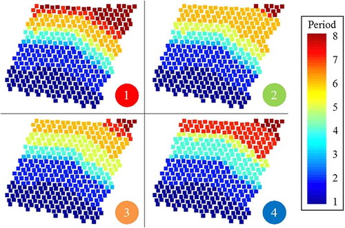
Figure 8. Comparison of the annual tonnage extraction for all four cases.

Note: The black line is the target.

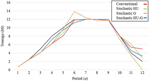
Figure 8 shows the annual extracted tonnages for all cases, where the black line indicates the mill target. Important to remark again is that the tonnages for the conventional (red) and the stochastic G (orange) cases are overly optimistic. The overtimes are so high that these forecasts are impossible to meet. However, it is also impossible to adjust these tonnages non-arbitrarily for the delays because it is not known how the slice extraction would move from period to period due to the overtime. This would have repercussions for the active draw points as well and then the whole schedule should be changed, which can only happen arbitrarily. Therefore, it is opted not to alter them, but to raise awareness that these forecasts will not be achieved. Figure 8 also shows that the stochastic HU and HU-G cases both meet the preset production targets while limiting the overtime in all periods. This emphasises, once again, the benefit of including the delays from hang-ups directly into the optimisation of the schedule. All schedules, except the stochastic G schedule, provide too much material in the final three periods of the life-of-mine. Recall that this is allowed since the mill constraints are modelled as soft constraints, and thus deviations are allowed (Constraints (12)). The reason for this increased production is that the tonnage targets in the final years are approximate targets of the demand. The demand reduces slightly from 12 Mt in period 9 because the number of active draw points is reduced in the later years so less production is to be expected. However, the exact tonnage that would be deliverable cannot be predicted in advance because it is schedule-dependent. This indicates that there is an option to increase the targets in the last years and reduce the mine life if desired. The stochastic G schedule, on the other hand, provides too much material in periods 6 and 7. This is probably caused by some high-grade areas extracted around that time in this schedule, and it does not represent an issue as this material can easily be stockpiled at the surface.

The tonnage targets are met while achieving the grade target in all the different cases. The inclusion of grade uncertainty in the optimisation does not have a high influence on this because the deposit in this case study is a very homogeneous, low grade copper deposit. The only influence from grade uncertainty is that the schedule is driven towards different zones earlier on, as illustrated in Figure 7. The same can be said for the BHOD. The BHOD is similar for all cases, usually more than half of the draw points are extracted up to the final limit of 512 metres. The only deviant case is the stochastic G schedule, where only grade uncertainty is considered. Here the optimiser leaves more material behind from the last draw points, in the top right corner of Figure 2, where the BHOD is only ±350 m. This is a result of deciding not to mine in the final period for this schedule, which is probably caused by lower grade material in that zone. The reason that this lower grade does not influence the stochastic HU-G case, which also includes grade uncertainty, is that in the stochastic HU-G case, this material is mined at the same time with material from other areas and thus the total average grade at the mill is different. The incorporation of the grade uncertainty is expected to have a higher influence on the BHOD and overall scheduling in a more traditional block caving deposit where the ore is capped by an in situ layer of waste rock. This transition zone would be quantified more accurately by the simulated grade models and, therefore, a higher difference is to be expected when compared to an optimisation that is based on an estimated model.

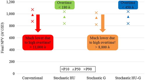
Figure 9 shows the risk analysis on the final NPV for the four different cases. In this figure, the boxes emphasise the incurred overtime and demonstrate for the conventional and stochastic G case that the NPV forecast is overly optimistic due to the high incurred overtimes. However, as mentioned, the earlier forecast cannot be adjusted for this in a non- arbitrary way. The forecasts for the stochastic HU and HU-G schedules are realistic because of the low overtimes, which are easily mitigated by daily schedule changes. Figure 9 also shows that the influence of the grade uncertainty is relatively low on the final NPV when the results of the optimised schedules of the stochastic HU and HU-G cases are compared in four scenarios. Their P10, P50 and P90 only marginally differ due to the homogeneity of the deposit, as pointed out earlier.

Figure 9. Comparison of the risk analysis of the final NPV for all four cases.

5. Conclusions

This paper addresses the long-term scheduling of block cave mines with the inclusion of hang-up delay uncertainty. Ignoring this uncertainty gave rise to overly optimistic schedule results, as demonstrated herein. This paper presents a novel approach to the long-term planning of block cave mines by explicitly including grade and hang-up uncertainty. The optimisation capitalises on this uncertainty and shows that the incorporation of the delays due to hang-up uncertainty strongly improves the results. Four different uncertainty scenarios are used to demonstrate the effectiveness of the presented optimisation formulation. The first scenario ignores uncertainty and the resulting ‘conventional’ schedule is rendered infeasible by conducting a risk analysis with hang-up scenarios. The same holds true for the second scenario with only grade uncertainty. In comparison, the third and fourth scenarios (one with only hang-up uncertainty, the other with both hang-up and grade uncertainty) lead to significantly better results. The schedules resulting from the optimisation of scenarios 3 and 4 easily meet production targets with minimal overtimes, which can be easily mitigated in short-term planning. The resulting schedules (from scenario 3 and 4) provide more accurate and, most importantly, feasible estimates of the projects’ NPV, which is critical to assessing accurately the economic feasibility. It is recommended that hang-up and other production delays are included in project schedule optimisation. The variability of their uncertainty is to be considered in the debottlenecking of tonnage, time schedule and production cost forecasts when examining the feasibility of a mineral resource project.

Future work on this topic is suggested to progress in two different paths, which, at some point, need to converge. The first would be to develop better solvers that are capable of tackling larger and more complex problems, such as metaheuristic solvers [32,41]. The second would be to develop models that incorporate more complex flows of the rock mass due to the excavation; this has potential to substantially improve the outcomes as compared to reality.

Disclosure statement

No potential conflict of interest was reported by the authors.

Funding

This work was supported by the Natural Sciences and Engineering Research Council of Canada (NSERC) Discovery [grant number 239019], [grant number 249942]; and the COSMO Mining Industry Consortium (AngloGold Ashanti, Barrick Gold, BHP Billiton, De Beers Canada, Kinross Gold, Newmont Mining and Vale) supporting the COSMO laboratory.

Acknowledgements

We thank the organisations that funded this research: The Natural Sciences and Engineering Research Council of Canada (NSERC) Discovery grant 239019 of Prof. Dimitrakopoulos, (NSERC) Discovery grant 249942 of Prof. Kazakidis, and the COSMO Mining Industry Consortium (AngloGold Ashanti, Barrick Gold, BHP Billiton, De Beers Canada, Kinross Gold, Newmont Mining and Vale) supporting the COSMO laboratory.

References

- S. Nadolski, B. Klein, D. Elmo, and M. Scoble, Cave-to-mill: A mine-to-mill approach for block cave mines, Min. Technol. 124(1) (2015), pp. 47–55.10.1179/1743286315Y.0000000001
- E. Chanda, An application of integer programming and simulation to production planning for a stratiform ore body, Min. Sci. Technol. 11(2) (1990), pp. 165–172.10.1016/0167-9031(90)90318-M
- A. Guest, G. Van Hout, A. Von Johannides, and L. Scheepers, An application of linear programming for block cave draw control. In Proceedings of the 3rd International Conference & Exhibition on Mass Mining, 2000, pp. 461–468.
- D. Rahal, M. Smith, G. Van Hout, and A. van Johannides, The use of mixed integer linear programming for long term scheduling in block caving mines. In Proceedings of the 31st International Symposium on the Application of Computers and Operations Research in the Minerals Industries, 2003, pp. 123–131.
- Y. Pourrahimian, H. Askari-Nasab, and D. Tannant, A multi-step approach for block-cave production scheduling optimization, Int. J. Min. Sci. Technol. 23(5) (2013), pp. 739–750.
- Y. Pourrahimian and H. Askari-Nasab, An application of mathematical programming to determine the best height of draw in block-cave sequence optimisation, Min. Technol. 123(3) (2014), pp. 162–172.10.1179/1743286314Y.0000000061
- F. Khodayari and Y. Pourrahimian, Mathematical programming applications in block-caving scheduling: A review of models and algorithms, Int. J. Min. Min. Eng. 6(3) (2015), pp. 234–257.10.1504/IJMME.2015.071174
- T. Diering, O. Richter, and D. Villa, Block cave production scheduling using pcbc. In Proceedings of the SME Annual Meeting & Exhibit 2010, 2010, pp. 455–467, Phoenix, Arizona.
- P. Dowd, Risk assessment in reserve estimation and open-pit planning, Trans. Inst. Min. Metall., Sect. A 103 (1994), pp. A148–A154.
- P.J. Ravenscroft, Risk analysis for mine scheduling by conditional simulation, Trans. Inst. Min. Metall. Sec. A 101 (1992), pp. A104–A108.
- S. Malaki and Y. Pourrahimian, Footprint calculation for block cave mining under grade uncertainty, Research Report 6 – Unpublished, Mining Optimization Laboratory, University Of Alberta, Edmonton, 2015.
- E. Vargas, N. Morales, and X. Emery, Footprint and economic envelope calculation for block/panel caving mines under geological uncertainty, 4th International Seminar on Mine Planning, Presentation, 2015. Available at https://www.researchgate.net/publication/281639806_Footprint_and_Economic_Envelope_Calculation_for_BlockPanel_Caving_Mines_Under_Geological_Uncertainty.
- R. Dimitrakopoulos and N. Grieco, Stope design and geological uncertainty: Quantification of risk in conventional designs and a probabilistic alternative, J. Min. Sci. 45(2) (2009), pp. 152–163.10.1007/s10913-009-0020-y
- S. Carpentier, M. Gamache, and R. Dimitrakopoulos, Underground long-term mine production scheduling with integrated geological risk management, Min. Technol. 125(2) (2016), pp. 93–102.10.1179/1743286315Y.0000000026
- L. Montiel, R. Dimitrakopoulos, and K. Kawahata, Globally optimising open-pit and underground mining operations under geological uncertainty, Min. Technol. 125(1) (2016), pp. 2–14.10.1179/1743286315Y.0000000027
- M. Godoy, The effective management of geological risk in long-term production scheduling of open pit mines, PhD thesis, The University of Queensland, Brisbane, Qld, 2002.
- M. Spleit and R. Dimitrakopoulos, Risk management and long-term production schedule optimization at the LabMag iron ore deposit in Labrador, Canada, Min. Eng. 69(10) (2017).
- R. Dimitrakopoulos, Stochastic optimization for strategic mine planning: A decade of developments, J. Min. Sci. 47(2) (2011), pp. 138–150.
- C.V. Deutsch and A.G. Journel, GSLIB: Geostatistical software library and user’s guide, Oxford University Press, New York, NY, 1992.
- P. Goovaerts, Geostatistics for natural resources evaluation, Oxford University Press, Oxford, 1997.
- N. Remy, A. Boucher, and J. Wu, Applied geostatistics with SGeMS: A user’s guide, Cambridge University Press, Cambridge, 2009.10.1017/CBO9781139150019
- I. Minniakhmetov and R. Dimitrakopoulos, Joint high-order simulation of spatially correlated variables using high-order spatial statistics, Math. Geosci. 49(1) (2017), pp. 39–66.10.1007/s11004-016-9662-x
- E. Rubio and S. Dunbar, Integrating uncertainty in block cave production scheduling, In Proceedings 32nd International Symposium on the Application of Computers and Operations Research in the Mineral Industry, 2005, pp. 635–642.
- E. Rubio and S. Troncoso, Discrete events simulation to integrate operational interruption events in block cave production scheduling, In Proceedings of the 3rd International Conference on Mining Innovation, 2008.
- S.N. Ngidi and D.D. Pretorius, Impact of poor fragmentation on cave management, In Proceedings 6th Southern African Base Metals Conference 2011, The Southern African Institute of Mining and Metallurgy, 2011, pp. 111–122.
- S. Ramazan and R. Dimitrakopoulos, Production scheduling with uncertain supply: A new solution to the open pit mining problem, Optim. Eng. 14(2) (2013), pp. 361–380.10.1007/s11081-012-9186-2
- L. Montiel and R. Dimitrakopoulos, Optimizing mining complexes with multiple processing and transportation alternatives: An uncertainty-based approach, Eur. J. Oper. Res. 247(1) (2015), pp. 166–178.10.1016/j.ejor.2015.05.002
- R.C. Goodfellow and R. Dimitrakopoulos, Global optimization of open pit mining complexes with uncertainty, Appl. Soft Comput. 40 (2016), pp. 292–304.10.1016/j.asoc.2015.11.038
- D. Laubscher, Cave mining-the state of the art, J. South Afr. Inst. Min. Metall 94(10) (1994), pp. 279–293.
- R. Dimitrakopoulos and S. Ramazan, Stochastic integer programming for optimising long term production schedules of open pit mines: Methods, application and value of stochastic solutions, Min. Technol. 117(4) (2008), pp. 155–160.10.1179/174328609X417279
- J. Benndorf and R. Dimitrakopoulos, Stochastic long-term production scheduling of iron ore deposits: Integrating joint multi-element geological uncertainty, J. Min. Sci. 49(1) (2013), pp. 68–81.10.1134/S1062739149010097
- R.C. Goodfellow and R. Dimitrakopoulos, Simultaneous stochastic optimization of mining complexes and mineral value chains, Math. Geosci. 49(3) (2017), pp. 341–360.10.1007/s11004-017-9680-3
- R. Dimitrakopoulos and S. Ramazan, Uncertainty based production scheduling in open pit mining, Trans. Soc. Min. Metall. Explor. 316 (2004), pp. 106–112.
- L. Caccetta and S.P. Hill, An application of branch and cut to open pit mine scheduling, J. Global Optimiz. 27(2/3) (2003), pp. 349–365.10.1023/A:1024835022186
- E. Topal, Early start and late start algorithms to improve the solution time for long-term underground mine production scheduling, J. South Afr. Inst. Min. Metall. 108(2) (2008), pp. 99–107.
- C. Cullenbine, R.K. Wood, and A. Newman, A sliding time window heuristic for open pit mine block sequencing, Optimiz. Lett. 5(3) (2011), pp. 365–377.10.1007/s11590-011-0306-2
- A. Lamghari and R. Dimitrakopoulos, Progressive hedging applied as a metaheuristic to schedule production in open-pit mines accounting for reserve uncertainty, Eur. J. Oper. Res. 253(3) (2016), pp. 843–855.10.1016/j.ejor.2016.03.007
- A. Boucher and R. Dimitrakopoulos, Block-support simulation of multiple correlated variables, Math. Geosci. 41(2) (2009), pp. 215–237.10.1007/s11004-008-9178-0
- R. A. Gonzalez Iturriaga, Desarrollo de flowsim 3.0: Simulador de flujo gravitacional para mineria de block/panel caving, Master’s thesis, Universidad de Chile, Santiago, 2014.
- S. Kenzap and V. Kazakidis, Simulation of operating risk in mine feasibilities, Trans. Soc. Min. Metall. Explor. 330 (2011), pp. 591–597.
- A. Lamghari and R. Dimitrakopoulos, A diversified Tabu search approach for the open-pit mine production scheduling problem with metal uncertainty, Eur. J. Oper. Res. 222(3) (2012), pp. 642–652.10.1016/j.ejor.2012.05.029