A monotone approximation for a size-structured population model with a generalized environment

Abstract

We study a nonlinear size-structured population model with an environment general enough to include hierarchy. We also remove the standard requirement that individuals have nonnegative growth rates, which allows the modeling of populations in which individuals may experience a reduction in size. To show existence and uniqueness of the solution to the model, we establish a comparison principle and construct monotone sequences. A fully discretized numerical scheme based on these monotone sequences is presented and utilized to provide some numerical examples.

Keywords:

• Size-structured population model
• Generalized environment
• Negative growth rates
• Monotone approximation
• Existence-uniqueness
• Numerical simulations

1. Introduction

Size and age structured population models have been a popular area of research over the past three decades 1–7. Most of these investigations have focused on the case where the vital rates depend on the total population. Since hierarchical rankings can play an important role in biological populations 8, some recent studies 6 9 10 have examined the case where these rates are dependent on a hierarchy which is established in the population. A common example of such a population is trees in a forest, where the competition for light that a given individual experiences comes only from individuals with the same or greater height, not the total population. The two cases mentioned above are in some sense the two extremes, i.e. in one, the competition is with the entire population and in the other, the competition is only with individuals with larger size. Between these two extremes, there can be competition with the entire population, while those with smaller sizes have a less significant effect.

In this paper, we study the following size-structured population model:

Here u(x, t) denotes the density distribution of a population of size x at time t, and the environment, Q(u)(x, t), a function of the density u, is given by

This definition of an environment is a generalization of those in 3 6 11. The functions and are, respectively, the mortality and birth rates of an individual of size x at time t and are dependent upon the environment. The function g(x, t) represents the growth rate of an individual of size x at time t, and γ(x, y) is a kernel used to define a given environment. We also assume that the population has a maximum size l<∞.

We chose to define the environment Q(u)(x, t) so that all the cases discussed above are covered. Note that for trees we could choose

and for the more general case in 9 we have

where . Note that if α=1, then Q(x, t)=P(t) is the total population. We present another example of how γ can be chosen to fit a given population in section 4.

Another uncommon feature of (1) is that we do not require individuals to have nonnegative growth rates. This allows the modeling of populations where individuals may experience a size reduction which may happen, for example, during a resource shortage.

Our approach for obtaining existence-uniqueness as well as for approximating solutions of (1) is in the spirit of those in 1 9 12 13. The analysis therein is based on the development of a comparison principle and the construction of a monotone approximation. This method has been successfully applied to many nonlinear differential equations 14–16 and is generally quite robust. However, for certain nonlocal nonlinearities, such as those in (1), the comparison principle based on the usual definition of upper and lower solutions fails 12. This difficulty is overcome by redefining the upper and lower solutions in a coupled form. With this new definition, we are able to establish a comparison principle and thus construct monotone sequences of upper and lower solutions which, upon passing to the limit, provide existence of a solution to (1).

The paper is organized as follows. In section 2 we establish a comparison principle and obtain uniqueness of solutions. Further, we construct monotone sequences and show how they converge to the solution of (1). In section 3 we discuss how one can discretize the monotone scheme in order to approximate solutions to (1). Finally, in section 4 we provide some examples and numerical simulations based on the approximations in sections 2 and 3.

2. The comparison principle, monotone approximation and existence-uniqueness of the solution

Throughout the paper we make the following assumptions on our parameters. The notation m _Q and β _Q will be used to denote and , respectively.

•  (A1) m(x, t, Q) is nonnegative and . Furthermore, m is locally Lipschitz with respect to Q and a.e.

•  (A2) is nonnegative and . Also, β is locally Lipschitz with respect to Q and a.e.

•  (A3) u ₀(x) is nonnegative and .

•  (A4) . Furthermore, g(0, t)>0 and g(l, t)=0 for 0≤t≤T.

•  (A5) γ(x, y) is nonnegative and

We begin by defining what we mean by a solution to (1). Let . We say that u(x, t) is a solution to (1) if and for every t∈(0, T) and every

We can now introduce the definition of coupled upper and lower solutions of (1).

Definition 2.1

A pair of functions and are called an upper and a lower solution of (1) on D _T , respectively, if all of the following hold.

• (i) 

• (ii)  a.e. in (0, l).

• (iii) For every t∈(0, T) and every nonnegative ,

With the definition given above, we can establish the following comparison principle.

Theorem 2.2

Suppose that (A1)−(A5) hold. Let and u be nonnegative upper and lower solutions of (1), respectively. Then a.e. in D _T .

Proof

Let and choose a nonnegative . Then w satisfies

and

Now choose and λ>0 so that on D _T . Let . Then we find

Now consider the following backward problem:

where and The existence of follows from the fact that by the variable change τ=t−s, (9) can be written as

Further, one can deduce from the initial data that on D _T . After substituting such a ζ into (8) and observing that we obtain

where

Now from the condition on the initial data in (6), we have

Since this equation holds for every χ, we can choose a sequence {χ _k } on (0, l) converging to

It then follows that

which by Gronwall's inequality yields

and the proof is complete.    ▪

We are now in a position to establish the following uniqueness result.

Theorem 2.3

Suppose that (A1)–(A5) hold. Then problem (1) has at most one solution.

Proof

Let u=u ₁−u ₂ be the difference of two solutions of (2). Then u satisfies

Choose such that

Here , and hence Substituting such a ξ into (12) and recalling that we have

where

This inequality is independent of χ˜, and so we can choose a sequence on (0, l) converging to

Consequently, we have

Now applying Gronwall's inequality yields

which is the desired result.    ▪

We now proceed to construct sequences of upper and lower solutions. Let . Choose a constant μ large enough so that

Fix this μ and choose δ large enough so that . Finally, choose γ so that

Let . Then it can be easily shown that and are a pair of coupled lower and upper solutions of (1) on D _T . Next we obtain two sequences and as follows.

For k=1, 2, … let and satisfy the system

and

Existence and uniqueness of solutions to (15) and (16) follow from the fact that they are both linear problems with local boundary conditions (also see 17). Further, by an argument similar to that in 9, we obtain two monotone sequences that satisfy

for each k=1, 2, … Since the sequences and are monotone, it follows that there exist functions u and such that and pointwise in D _T . Clearly a.e. in D _T . We now show that . To this end, let . Since , w(x, t)≥0 and from (15)–(16), w(x, 0)=0. Integrating (15)–(16) and then letting gives

where

It now follows from Gronwall's inequality that w(x, t)=0, i.e. . If we define u to be this common limit, we find that u is the solution of (1). We can now state the following existence-uniqueness result.

Theorem 2.4

Suppose that (A1)−(A5) hold. Then there exist monotone sequences and which converge to the unique solution of (1).

3. Implementation of the numerical scheme

In this section, we elaborate on how one can implement the numerical scheme given by (15)–(16). Many other approaches 18–26 have been taken to obtain numerical solutions of population models, although none have considered the generalized environment in (1). Our approach is based on a combination of the standard method of characteristics and the scheme discussed in the previous section. Each characteristic curve satisfies

Therefore, the solution of (15) satisfies

along a characteristic curve (t(s), x(s)). It is clear that the existence of a unique solution of (18) follows from assumption (A4). If we parameterize the characteristic curves with the variable t, then a characteristic curve passing through the point is given by , where X satisfies

Now let be the inverse relation of the function Define . Then (x, G(x)) represents the characteristic curve emanating from the origin and dividing the (x, t)-plane into two regions. For any point (x, t) with t≤G(x), the solution is determined through the initial condition by

On the other hand, if t>G(x), then the solution is determined via the boundary condition by

where

Note that the contribution of the monotone approximation lies in the fact that since the system defined by (15) and (16) is linear, (21) and (22) are explicit representations of .

It is worth mentioning that although Γ is not a well-defined function, is a unique number for each (x, t) with t>G(x) since we assume in (A4) that g(0, t)>0. A similar representation can be derived for the solution by interchanging and in (21) and (22).

We can now discretize the region , and hence the solution representations for and . Choose two integers m, n>1. Define and . Now let and for . Similarly, let for . With the points and we have discretized the bottom and left boundaries of D _T , respectively. Using an appropriate numerical method, (we used the classical 4th order Runge–Kutta method with Δ t as our step size) one can easily produce m+n−1 (one for each and ) characteristics by solving the following differential equations:

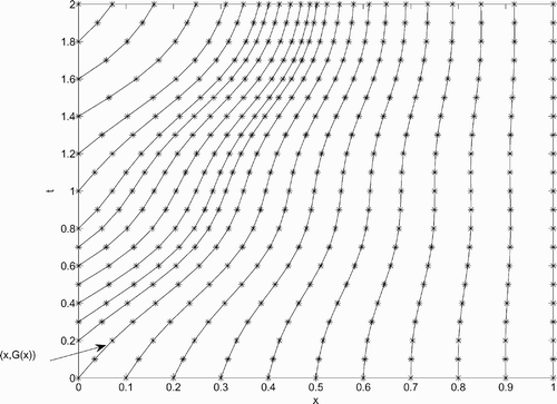
At this point we have a set of discrete points in at which the solutions and will be approximated. An example of output from (23) is shown in figure 1.

Figure 1. Discretized characteristics in D _T .

Denote each discrete characteristic emanating from the initial condition by , corresponding to , and each discrete characteristic emanating from the boundary by , corresponding to . Notice that and that while each consists of n values, consists of n−i values. Denote each of these values by and . To approximate at each of these values, it is convenient to define to be the sth point along the rth time step. Here r=1, …, n and s=1, … m+r. Then for s>1 we can approximate with a right Riemann sum as follows:

A similar procedure can be used to approximate .

Now let . Then for the points we have

and for the points we have

Again, a similar procedure can be used to calculate .

In order to test our method, we chose the following vital rates:

with the initial condition . We also chose , which implies that is the total population. Now if we consider the quantity , which is commonly known as the total biomass of the population, and integrate (1), we obtain the following ODE:

In a similar manner, multiplying the PDE in (1) by x and integrating gives:

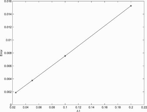
We used MATLAB's ode45 routine to solve (27) and (28) and compared the results with our method. We fixed and used our method to calculate P(t) with and 0.2. Further, we chose T=4, l=1 and k=1, 2, … 15. Our initial upper and lower solutions were and . We then calculated the error associated with Δ t as the maximum difference between our upper and lower total populations and the total population calculated with ode45. Figure 2 suggests that the method is first order with respect to the step sizes.

Figure 2. Error analysis.

4. Applications

In this section, we apply (1) to two specific problems to show how the generalization of Q(u)(x, t) and the relaxed conditions on the parameters of the model have practical value. For each application, we present the numerical solution of (1) obtained from the methods discussed in section 3.

4.1 Populations which undergo metamorphosis

Many populations, such as frogs and butterflies, undergo the process of metamorphosis. Although individuals at each stage are technically of the same species, competition between stages is often negligible. For example, frogs and tadpoles have completely different food sources. In this section we will consider the frog–tadpole example. Since little dynamics take place at the egg stage, we choose not to model this stage explicitly. We first assume that T=2 and all parameters have been scaled so that tadpoles have sizes in the range 0≤x<0.5 and frogs have sizes in the range 0.5≤x<1. Since frogs do not compete with tadpoles, we chose γ(x, y) so that

This is achieved by letting

When considering the fact that only frogs give birth, we choose as follows

The factor is chosen to mimic the frogs periodic birth rate. For the death rate we choose

The death rate is chosen to be constant while the population remains small and to increase linearly when the population becomes larger than the carrying capacity of the environment. We are essentially modeling an area that can sustain 50 tadpoles and 5 frogs. The growth rate and initial population are chosen to be g(x, t)=1 and . For the steps sizes we used and with . We chose and . Note by choosing g(x, t)=1 the model becomes age structured. Also we chose , and . 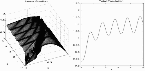In figure 3 we show the plots of the lower solution after 20 iterations and the total population of frogs.

Figure 3. (Left) Approximate lower solution after 20 iterations (u ²⁰). (Right) The total population after 20 iterations (Q(u ²⁰)).

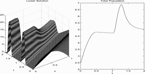
Notice that the increases in the total frog population shown in figure 3 occur shortly after the breeding seasons. It is also worth mentioning that , indicating the rapid convergence of the method.

4.2 Periodic resource shortages

Many populations live in environments that subject them to extended periods of scarce resources. Examples might be long, cold winters or long dry seasons. In both cases, individuals of a species are likely to experience some reduction in size. In order to model this situation, one must remove the common condition that g(x, t)≥0. To begin, we assume that T=5 and l=1. To represent the reduction of the size of individuals due to a seasonal resource shortage, we chose

This function is modeling a situation where the largest 25% of the population periodically experiences some reduction in their size. We chose the death rate to be

Notice that this death rate is largest during the same time period where the resource shortage occurs. During this time period, we should also see low birth rates and so we chose

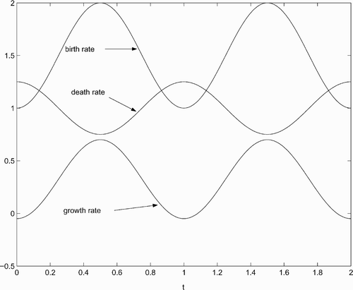
To illustrate the motivation for these particular choices of growth, birth and death, we show the plots of their periodic factors in figure 4 (we chose x=0.8 in the periodic factor of g(x, t)). Notice that the resource shortages occur at the integers. Hence at times t=0, 1, 2 growth and birth are at their minima and death is at its maximum. Notice also that g(x, t) periodically becomes negative, causing a reduction in size for certain individuals.

Figure 4. Periodic factors for growth, death and birth.

We assume that individuals compete equally with the entire population, and hence γ (x,y) = 1, which implies

For the initial population we chose and for the step sizes we used and with . Our initial upper and lower solutions were and . We show the numerical results in figure 5. Notice from figure 5 that the maxima of the total population occur just before the integers, which correspond to the worst time periods for the population. Figure 5 also suggests that the population approaches a periodic solution. Also, in figure 5 we see that the individuals with x≥0.75 periodically reduce in size, as expected.

Figure 5 (Left) Approximate lower solution after 20 iterations (u ²⁰). (Right) The total population after 20 iterations (Q(u ²⁰)).

Acknowledgements

The work of A.S. Ackleh was supported in part by the National Science Foundation under grants DUE-0531915 and DMS-0718465. The work of K. Deng was supported in part by the National Science Foundation under grant DMS-0718465.

References

- Ackleh , A. S. and Deng , K. 2000 . Existence-uniqueness of solutions for a nonlinear nonautonomous size-structured population model: an upper-lower solution approach . Canadian Applied Mathematics Quarterly , 8 : 1 – 15 .
- Calsina , A. and El odrissi , O. 2002 . Asymptotic behavior of a semilinear age-structured population model with a dynamics for the resource . Mathematical, Computer Modeling , 35 : 403 – 427 .
- Calsina , A. and Saldana , J. 1997 . Asymptotic behavior of a model of hierarchically structured population dynamics . Journal of Mathematical Biology , 35 : 967 – 987 .
- Clemons , C. B. , Hariharan , S. I. and Quinn , D. D. 2001 . Amplitude equations for time-dependent solutions of the McKendrick equations . SIAM Journal of Applied Mathematics , 62 : 684 – 705 .
- Gurtin , M. and MacCamy , R. C. 1974 . Nonlinear age-dependent population dynamics . Archive for Rational Mechanics and Analysis , 54 : 281 – 300 .
- Kraev , E. A. 2001 . Existence and uniqueness for height structured hierarchical population models . Natural Resource Modeling , 14 : 45 – 70 .
- Tucker , S. I. and Zimmerman , S. O. 1988 . A nonlinear model of population dynamics containing an arbitrary number of continuous structure variables . SIAM Journal of Applied Mathematics , 48 : 549 – 591 .
- Lomnicki , A. 1998 . Population Ecology of Individuals, Monographs in Population Biology, 25 , Princeton : Princeton University Press .
- Ackleh , A. S. and Deng , K. 2005 . Monotone approximation for a hierarchical age-structured population model . Continuous and Discrete Impulse Systems Series B , 12 : 203 – 214 .
- Cushing , J. 1994 . The dynamics of hierarchical age-structured populations . Journal of Mathematical Biology , 32 : 705 – 729 .
- Ackleh , A. S. , Deng , K. and Hu , S. 2005 . A quasilinear hierarchical size-structured model: well-posedness and approximation . Applied Mathematics and Optimization , 51 : 35 – 59 .
- Ackleh , A. S. and Deng , K. 1997 . Monotone method for first order nonlocal hyperbolic initial-boundary value problems . Applicable Analysis , 67 : 283 – 293 .
- Ackleh , A. S. and Deng , K. 2000 . A monotone approximation for a nonlinear nonautonomous size-structured population model . Applied Mathematics and Computation , 108 : 103 – 113 .
- Bellman , R. 1973 . Methods of Nonlinear Analysis , Vol. II , New York : Academic Press .
- Ladde , G. S. , Lakshmikantham , V. and Vatsala , A. S. 1985 . Monotone Iterative Techniques for Nonlinear Differential Equations , Boston : Pitman .
- Pao , C. V. 1992 . Nonlinear Parabolic and Elliptic Equations , New York : Plenum Press .
- Ackleh , A. S. and Deng , K. 1999 . A monotone approxiamtion for the non-autonomous size-structured population model . Quarterly Applied Mathematics , 57 : 261 – 267 .
- Abia , L. M. , Angulo , O. and López-Marcos , J. C. 2004 . Size-structured population dynamics models and their numerical solutions . Discrete and Continuous Dynamical Systems Series Ba , 4 : 1203 – 1222 .
- Ackleh , A. S. and Ito , K. 1997 . An implicit finite difference scheme for the nonlinear size-structured population Model . Numerical Functional Analysis and Optimization , 18 : 865 – 884 .
- Angulo , O. and López-Marcos , J. C. 2004 . Numerical integration of fully nonlinear size structured population models . Applied Numerical Mathematics , 50 : 291 – 327 .
- Angulo , O. and López-Marcos , J. C. Numerical integration of a size-structured cell population model in an environment of changing substrate concentration . Proceedings of the International Conference on Computational Methods in Sciences and Engineering . Kastoria, Greece. Vol. 1 , pp. 28 – 32 .
- Fairweather , G. and López-Marcos , J. C. 1994 . An explicit extrapolated box scheme for the Gurtin–MacCamy equation . Computers & Mathematics with Applications , 27 : 41 – 53 .
- Ito , K. , Kappel , F. and Peichl , G. 1991 . A fully discretized approximation scheme for size-structured population models . SIAM Journal of Numerical Analysis , 28 : 923 – 954 .
- Kostova , T. 2003 . An explicit third-order numerical method for size-structured population equations . Numerical Methods for Partial Differential Equations , 19 : 1 – 21 .
- Sulsky , D. 1993 . Numerical solution of structured population models, I, Age structure . Journal of Mathematical Biology , 31 : 817 – 839 .
- Sulsky , D. 1994 . Numerical solution of structured population models, II, Mass structure . Journal of Mathematical Biology , 32 : 491 – 514 .