Ecology and evolution of symbiosis in metapopulations

Abstract

We present a model for symbionts in plant host metapopulation. Symbionts are assumed not only to form a systemic infection throughout the host and pass into the host seeds, but also to reproduce and infect new plants by spores. Thus, we study a metapopulation of qualitatively identical patches coupled through seeds and spores dispersal. Symbionts that are only vertically inherited cannot persist in such a uniform environment if they lower the host's fitness. They have to be beneficial in order to coexist with the host if they are not perfectly transmitted to the seeds; but evolution selects for 100% fidelity of infection inheritance. In this model we want to see how mixed strategies (both vertical and horizontal infection) affect the coexistence of uninfected and infected plants at equilibrium; also, what would evolution do for the host, for the symbionts and for their association. We present a detailed classification of the possible equilibria with examples. The stability of the steady states is rigorously proved for the first time in a metapopulation set-up.

Keywords:

• metapopulation dynamics
• equilibrium
• coexistence equilibrium
• stability
• fitness
• invasion fitness

1. Introduction

There are many examples of symbiotic associations with plant hosts in nature.

• Rhizobia are nitrogen fixing bacteria in soil that form root nodules on legume plants. The legume–rhizobium symbiosis is a classic example of mutualism; rhizobium provides amino acids to the plant, which in turn supplies the rhizobia with organic acids that are a source of carbon and energy for the bacteria. Rhizobia inoculants are used for legume cultures when a nitrogen fertilizer is not used. [6,7 

• Trichoderma are free-living fungi in soil. They are recognized agents for plant-disease control, for their ability to increase plant growth and development, and are widely used in horticulture. They are opportunistic, avirulent plant symbionts and parasites to other fungi. [3 

• Mycorrhizae are ubiquitous symbiotic associations of plant roots and certain soil fungi. They are present in more than 95% of all plant species. [1 

• Endophytic fungi live internally and asymptomatically within plant tissues–occurring in above-ground tissue and also occasionally in roots, but lacking in external hyphae as mycorrhiza has. They range from fungal plant pathogens and saprophytes to specialized grass fungi that are considered as mutualists. [2,4,5,24,30,32 

• Epiphytes are plants that grow upon another living plant. They are usually non-parasitic on their host, growing independently and deriving only physical support (mosses, lichens, orchids); but there are also parasitic and semiparasitic epiphytes such as mistletoe. [28,33 

Most of these plant symbiont associations are mutualistic (rhizobia, mycorrhiza, trichoderma), horizontally spread and appear to be stable 25 26 34.

Numerous studies have shown that vertically transmitted symbionts should be non-parasitic in order to persist 14 15 23, as their reproductive success relies entirely on the host's fitness, while horizontally transmitted symbionts are usually pathogens decreasing their host's fitness. Also, symbionts with different reproductive strategies may coexist on the same host when they exploit different ecological niches 25 – vertically transmitted symbionts exploit their host's capacity to reproduce, while horizontally transmitted ones exploit their survival capacity.

In this paper, we develop a mathematical model that is primarily designed for endophytic symbiosis, where symbionts have a mixed reproduction strategy, but the methodology may easily be applied to any kind of symbiotic association.

Most of the natural plant populations have a patchy spatial structure. With this kind of habitat fragmentation, the population becomes a network of local populations interconnected through dispersal, a so-called metapopulation 21 22. The model is formulated and analysed for possible steady states in Section 2. We work in the cumulative framework developed in 8–13,18 19. We present a detailed classification by degree of infection transmission fidelity for the possible solutions of the steady-state problem. Then, in the next section, we present the stability analysis of the equilibria. In Section 4, we give invasion criteria for different set-ups – invasion in a virgin environment, invasion of the symbiont in a symbiont-free metapopulation and invasion of a mutant symbiont in a coexisting infected – susceptible plant metapopulation at equilibrium. The trait undergoing selection is the the fidelity of the vertical transmission. Some examples are presented in Section 5, followed by concluding remarks in the last section.

2. Model description and analysis

Several simplifying assumptions are made in order to reduce the model's complexity, nonetheless they are not unrealistic and allow for both mathematical analysis and biological insight. We consider a metapopulation with infinitely many identical patches of carrying capacity K that are equally coupled through dispersal. 16 18 19

Local populations may become extinct due to random catastrophes (occurring at a rate ϵ) after which the patch is recolonized by dispersers arriving from a dispersal pool. Each habitable patch supports a local population of age of coexisting symbiont infected plants with density i(a) and symbiont uninfected plants with density s(a). The age of the local population is the time elapsed since the last extinction–colonization event.

We assume the per capita mortality rates μ _s , μ _i and per capita fertility rates γ _s , γ _i of the susceptible and infected plants are density independent. The biomass of symbionts living within the host tissue grows with the infected plant and passes into the seeds. The newly produced seeds of both the infected and susceptible plants enter the dispersal pool and will eventually migrate into a new patch at rate α, or die during dispersal with per capita rate ν. Thus, they survive migration with probability

A proportion p of the seeds proceeding from one infected plant is infected, while the rest of (1−p) remains symbiont free. The fidelity of vertical transmission may be an attribute of either the plant or the symbiont. The plant may hinder the symbiont's transfer into all the seeds, or some of the infected seeds may lose their infectivity while they are dormant in the seed bank. On the other hand, the symbiont strives to infect as many seeds as possible. When p=0 the symbiont is transmitted only horizontally to new plants, when p=1, there is a 100% fidelity of the vertical transmission of the infection, whereas the intermediate values of p∈(0, 1) correspond to the mixed strategy symbionts.

We assume that symbionts sporulate with per host capita rate σ. Spores are globally dispersed by pollinators or wind, being exposed to a death risk at per spore rate η, and will enter a local population at rate β. Thus, they survive dispersal with probability . Once they are in a local patch, they infect new susceptible plants at a contact rate C, otherwise they die.

At a certain moment of time t, we have densities for uninfected and infected seeds, and density D _sp(t) for spores in the dispersal pool.

Although death and birth are density independent phenomena, we still account for local competition, namely for germination sites. Seeds entering a local population of age a germinate with probability , if they are not infected or , if they are infected.

The local population dynamics at time t of a local population with age a is described by the ODE system

If the metapopulation is at a steady state, the densities in the dispersal pool become constant and the local dynamics is governed by the linear differential equations with constant coefficients

Then one can solve the initial value problem for an empty patch ($s(0)=0,i(0)=0$) and get the solution

where are the eigenvalues (depending on ) associated with system (1). If a long enough time is allowed for the local population's dynamics, the local densities approach the equilibrium values. However, local catastrophes that happen with constant rate ϵ obstruct the progress of the local population towards equilibrium. When a catastrophe occurs the local population is completely destroyed, but the patch remains habitable and it is immediately recolonized by new seeds continuously arriving from the dispersal pool. In fact, the local catastrophes are the only ingredient that gives the system the metapopulation structure. Because dispersal is assumed to be global and uniform and the patches are identical, all local populations would reach the unique equilibrium (s*, i*), and the metapopulation would behave as one well-mixed population, if catastrophes were absent.

Given that local catastrophes may occur, the metapopulation consists of many local populations with different ages (time since the last catastrophe of the patch) and it is fully characterized by the age distribution of the local populations

The questions we address are concerned with invasion of the metapopulation in a virgin environment, invasion of a symbiont in the symbiont-free plant metapopulation, and, more importantly, the metapopulation as well as the symbiont persistence at equilibrium and the evolution of the symbiont. The formulation of the general deterministic nonlinear structured population models developed by Diekmann et al. 8–13 and adapted to metapopulation models by Gyllenberg et al. 17–19 befits particularly well these types of problems. Essentially, this formulation is based on the notion of environmental condition. At a steady state, the environmental condition is a constant; thus individuals are independent of one another and the equations become linear. The general form of the steady-state problem becomes

where the vector I describes the environmental condition, b is a vector of steady birth states, b - vector of steady birth states L - next generation operator!L(I)- in the general formulation L(I) is the next-generation-matrix (given the environmental condition I) I - input!I - environmental conditions in the general formulation and G(I) G(I) - feedback matrix is the feedback matrix describing the life-time contribution of an individual to the environmental conditions 10.

We choose the environmental variables to be the inflows of seeds and spores into the local patches. Thus, We are dealing with a metapopulation of plants, so our first thought would be to consider, as birth states, the infected and uninfected seeds. However, for the generation growth of the population, the adult state is important – when the plant is already established and may start producing seeds. We have a certain degree of freedom in choosing the renewal state of an individual (see 12). It has to pass the seed and seedling state before being able to reproduce, so the renewed individual is the adult plant.

The (i, j)–element of the next generation matrix L(I) is the expected number of offspring with renewal state i produced by an individual that itself had renewal state j, under environment I, whereas the (i, j)–element of the feedback matrix G(I) is the lifetime contribution to the ith component of I of an individual renewed in state j.

Consider one susceptible adult plant before the first reproductive burst – it will survive uninfected up to age a with probability and it will produce on average: seeds during its entire life, provided it is not horizontally infected. These seeds survive the dispersal with probability π and enter an arbitrary patch of age a, where they germinate with probability where is the age-distribution of the local population.

We reason similarly for all components of the matrices L(I), G(I) and introduce the following shorthand notations in order to avoid cumbersome formulas

where are the overall mortality rates of susceptible and infected plants, respectively.

Given one plant born uninfected, Q is the average lifetime seed production of this plant for as long as it stays uninfected. If it would become infected at a certain age, then H is the average life time production of seeds during the period of infection ((1−p) uninfected, p infected) and is the production of spores during the same period. Similarly, T is the average life time production of seeds and is the average life time production of spores for a plant that was born infected. With these simplifications, we get the next generation and the feedback matrices

The steady state problem is thus reduced to a system of two equations

Note that the first equation in system (8) is the equilibrium condition that the long-term growth rate of the metapopulation, which in our case is the dominant eigenvalue of the matrix L(I), is exactly one, therefore the metapopulation neither grows nor declines.

Let

be the expected numbers of new plants produced by one susceptible and one infected plant, respectively, during their entire lives in a virgin environment.

Solving the linear system (8), we get several solutions

• the trivial solution corresponding to metapopulation extinction,

• the symbiont-free metapopulation equilibrium provided R _s>1

• if p=1, which means 100% fidelity of vertical transmission of the infection, we get

  		which for R i>1 is the equilibrium for totally infected metapopulation,
  		if and there is an equilibrium in the interior of the positive orthant. This is biologically counterintuitive. One would expect totally infected metapopulation when vertical transmission is perfect and symbionts have mixed spreading strategy. In fact, the symbiont reduces the host's fitness so much that they would go extinct if they were only vertically transmitted, whereas the uninfected plants are fit enough to persist at equilibrium.

• if p=0 the infection spreads only via spores, and the possible equilibria are

  possibly one or two equilibria , where and I sp is a solution to the second degree equation if it is real and positive

• for p∈(0, 1) there are possibly one or two coexistence equilibria the positive solutions of the system below

where and are two hyperbolas

with coefficients

The coexistence equilibria of the metapopulation are the intersection points of the hyperbolas situated in the first quadrant. We have performed an exhaustive graphical analysis, which allows us to give conditions for the existence of one or two interior equilibria. This analysis is rather lengthy and is included as an appendix in 29.

For a fixed set of parameters, as p runs from 0 to 1, the equilibrium solution can bifurcate from the endophyte-free equilibrium to one or two coexistence equilibria that may persist or not for new values of p. We present several possible cases in Table 1. Later on, in Section 5, we show concretely how each case works together with the bifurcation and stability diagrams. Other combinations may be possible but the behaviour of the system is essentially similar.

Table 1. Interior equilibria and bifurcation by p.

Case 1
	There is no interior equilibrium
Case 2
	There is one interior equilibrium
Case 3	p∈[0, p 0)			p∈[p 0, 1]
	No equilibrium			One equilibrium
Case 4	p∈[0, p 0)	p = p 0	p∈(p 0, 1]
	No equilibrium	One equilibrium	Two equilibria
Case 5	p∈[0, p 1)	p = p 1	p∈(p 1, p 2)	p∈[p 2, 1]
	No equilibrium	One equilibrium	Two equilibria	One equilibrium

3. Stability analysis

In the previous chapters, we have studied our metapopulation solely for the existence of equilibria. However, to analyse stability of the equilibria we have found, we need to consider the bigger picture of the dynamics in a variable environment. Thus, if the metapopulation has not yet reached an equilibrium, the dispersal pool densities (environmental variables) are some given functions of time rather than constants.

A local population of age a at time t was established at time t − a. The dynamics of such a local population is described by the differential equations

for and the initial conditions We denote the solution of system (13) by , depending on the triplet The probability that a local population, survives to age a is By integrating over all possible ages of local populations we get a delay equation coupled with three differential delay equations describing the global dynamics of the metapopulation

where b(t) is the birth rate of local populations at time t.

At equilibrium we work again in a constant environment characterized by constant dispersers input and the whole system dynamics is governed by the Equations (2) and (8) previously studied in Section 2. The equilibrium condition for the birth rate equation becomes the identity:

This is due to the fact that at equilibrium, each local population exactly replaces itself (after a local catastrophe the patch is immediately recolonized), hence, the indeterminacy of b.

In order to check the stability of the equilibria we will study the linearized system and apply the principle of linearized stability that was proved rigorously in 8 9. The linearization of Equation (14) is done by plugging-in a small perturbation of the equilibrium

applying the Taylor expansion about the equilibrium and neglecting the higher order terms in , which are small. Thus, we obtain

Here and are the Fréchet derivatives with respect to each component of They are calculated by differentiating system (13) and solving the newly obtained systems in , for Then, taking the Laplace transform of Equation (16) we obtain

which can be written in matrix form

Shortly, in our case, the principle of linearized stability says that the equilibrium is stable if all the eigenvalues associated with the system have negative real part and it is unstable if there exists at least one eigenvalue with positive real part. The eigenvalues are the solutions of the characteristic equation

where the components of the matrix are

Obviously, λ=0 is always a solution of the characteristic equation due to the indeterminacy of b. Thus, the stability of the equilibrium is given by the position in the complex plane of the solutions of the equation:

where

For Equation (21) is equivalent to

with We can apply Nyquist's criterion (Corollary 2.20 in 9) to the new Equation (23). According to this criterion, the equilibrium is unstable if the curve winds counterclockwise at least once around the origin as ω runs from ∞ to −∞, and it is stable otherwise.

4. Invasion criteria

In a single population, fitness is defined either as the long-term exponential growth rate r(I), or equivalently, the basic reproduction ratio R(I), of a phenotype in a given constant environment I. Although r is the growth rate in real time, while R operates on generation basis, the two are equivalent in a constant environment – R is less than, equal to or greater than 1 when r is respectively less than, equal to or greater than 0.

In a structured metapopulation model, the fitness as defined by Gyllenberg and Metz 17 27, is the spectral radius (dominant eigenvalue) of the next generation operator (matrix L(I) in this model).

Assume that the resident metapopulation has reached an equilibrium – a constant distribution of age-structured local populations, corresponding to a constant environment I. Then, as discussed in Section 2, the resident fitness is 1 (the dominant eigenvalue of the matrix L(I) in Equations (7) and (8)). A rare mutant coming into the metapopulation will experience the environment as set by the resident and, because it is rare, it initially will not affect the resident equilibrium. If the fitness of the mutant is greater than 1 the mutant population grows when its size is small, and invades the resident metapopulation. As the size of the mutant population is small it is still possible that invasion will not happen due to demographic stochasticity.

The parameter p is the proportion of infected seeds produced by one infected plant. It accounts both for the success of the plant to bequest the symbiont when it is beneficial and for the success of the symbiont to persist in the metapopulation in spite of its parasitic effect upon the host. Thus, we may consider p as a trait of the plant or as a trait of the symbiont, alternatively.

If p is the trait of the infected plant, the fitness of the mutant plant with strategy p ^mut is the dominant eigenvalue, of its next generation matrix

Alternatively, if p is the symbiont's trait, we calculate the fitness of the mutant symbiont, defined as the expected number of new infected plants produced by one infected plant during its entire life, either offspring inheriting the infection or plants infected by spores

Here, is the age-distribution of local populations at equilibrium and are the densities of a resident local population in the constant environment The first component of the fitness is the contribution of the vertical infection transmission, whereas the second one is due to horizontal transmission.

4.1. Invasion in a virgin environment

To reach a non-trivial equilibrium the plant metapopulation should be able to grow in a virgin environment when it is still small, which formally means that given the next generation matrix

the metapopulation will invade the virgin environment if the dominant eigenvalue is greater than 1.

Note that the horizontal transmission of the infection plays no role in this invasion criterion and the present situation is identical to the model developed in 20 31 for only vertically transmitted endophytes. This is only natural – in a virgin environment, before the metapopulation is established, there are no plants to be infected by spores. The situation is different when we speak about invasion of a mutant in a resident plant population at equilibrium.

4.2. Invasion of a rare mutant

Assume that the metapopulation has reached an equilibrium such that both the susceptible and the infected plants are prevailing in the constant environment The resident plant and the resident symbiont have strategy p. A mutant infected plant with strategy p ^mut can invade if its invasion fitness is greater than 1. However the invasion fitness of the mutant plant may differ from the invasion fitness of a mutant symbiont. The symbiont would be able to invade if its invasion fitness defined in Equations (25),

is greater than 1. Moreover is a strictly increasing function of p ^mut, therefore the evolution of the symbiont will drive p towards its highest value 1 and the infection level of the metapopulation to 100%.

4.3. Invasion of the symbiont in a symbiont-free plant metapopulation

If a small symbiont-free population can grow and reach the symbiont-free equilibrium There are of course no infected seeds or spores present at this equilibrium. However, a symbiont with strategy p∈(0, 1] may be able to invade the metapopulation if it has invasion fitness

greater than 1. Thus, all symbionts with strategies

would be able to invade a symbiont-free metapopulation.

5. Examples

In this chapter we present illustrations of the possibilities we have described in Table 1. For each example we calculate the equilibria as shown in Section 2 and prove that they are stable or unstable using the method presented in Section 3 (Nyquist's criterion).

Case 1

No interior equilibria. For the following parameter set, the symbiont is not sustainable in the plant population.

Solving the equilibrium equation we get the unique solution corresponding to the symbiont-free metapopulation (Figure 1).

Figure 1. No interior equilibria. The symbiont-free equilibrium is stable and uninvadable for all values of p∈[0, 1].

The seed production of the infected plant and the germination success of the infected seeds are smaller than those of the uninfected plants, thus the symbiont decreases the host's fitness. The uninfected plant fitness, on the other hand, is so, a small symbiont-free population is able to grow and invade a virgin environment. Then, it will reach the stable symbiont-free equilibrium with . It is also evolutionarily stable. If a symbiont would come along, its invasion fitness, would be less than 1 for all p in [0, 1], so no invasion takes place.

Case 2

One coexistence equilibrium for all p∈[0, 1]

Suppose we have a symbiont-free metapopulation at equilibrium (Figure 2). This equilibrium is not stable and symbionts that only spread horizontally are able to invade. When few spores come into the metapopulation, they produce the first generation of infected plants, which despite its small size and its incapacity to produce infected seeds (p=0) will be able to contagiously infect new plants and grow. The metapopulation will reach a new equilibrium with coexisting susceptible and infected plants corresponding to the environment However, as soon as p becomes greater than 0 the infected plants will start producing infected seeds and we get a new interior equilibrium that is stable for all values of p>0.

Figure 2. The symbiont-free equilibrium is unstable. The unique coexistence equilibrium is stable for all values of p∈[0, 1]. Arrows indicate evolution of p as strategy of the plant or symbiont. The plant and the symbiont have opposite interest, their evolution pulls p in opposite senses.

As we have emphasized in Section 4.2, the symbiont will always try to increase p, but the fitness of the mutant plant is greater than 1 for all Therefore, there is a clear evolutionary conflict between the plant and the symbiont.

Interestingly, when p=1, infected and uninfected plants can still coexist . This may come as a surprise, but, for the same parameter set, in the model for exclusively vertically transmitted symbionts 20, the basic reproduction number of the infected plant was R _i=1/2, while R _s=2; thus, even when the transmission of the infection was perfect (p=1), the symbiont could not persist at equilibrium and the metapopulation became symbiont free. This clearly shows that, by attaining means of horizontal transmission, the symbiont escapes extinction although it lowers the host's fitness.

Case 3

No coexistence equilibrium for p∈[0, p ₀), one coexistence equilibrium for p∈[p ₀, 1],

For all p∈[0, 1], there is the symbiont-free equilibrium (Figure 3). This equilibrium is stable and uninvadable for but any symbiont with would perform well enough to be able to invade it because it is no longer stable. Thus, the metapopulation would reach a stable interior equilibrium. Moreover, the fitness of both the mutant plant and the mutant symbiont on the interior equilibrium is greater than 1 for all p>0.4584, so evolution drives p to value 1.

Figure 3. The symbiont-free equilibrium stable on [0, 0.4584) bifurcates to the unique stable coexistence equilibrium. Arrows indicate evolution of p as strategy of the plant or symbiont.

In this particular example, when p=1, the metapopulation becomes totally infected reaching the evolutionarily stable equilibrium This suggest that the symbiont-plant association is purely mutualistic as it benefits both the plant and the symbiont equally.

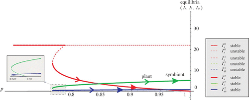
Case 4

p∈[0, p ₀) – no coexistence equilibrium, p = p ₀ one coexistence equilibrium, p∈(p ₀, 1]− two coexistence equilibria,

The equilibrium equation has three solutions: the symbiont-free equilibrium on [0,1] and two interior equilibria for p∈[0.9769, 1] (Figure 4). Applying the stability criterion, one can see that the symbiont-free solution is stable, the interior equilibrium is unstable, and is stable.

Figure 4. The symbiont-free equilibrium stable on [0,1]. Two interior equilibria on [0.9769,1], one stable, one unstable. Arrows indicate evolution of p as strategy of the plant or symbiont. Evolutionary conflict between plant and symbiont on [0.9769,0.99553], agreement on [0.99553,1].

Suppose the metapopulation is at the stable symbiont-free equilibrium. Then,

which is strictly less than 1 for all This means that the symbiont-free equilibrium is also evolutionarily stable.

There exists, however, a stable interior equilibrium Looking at the fitness of a mutant plant, we note that p=0.99553 is a singular strategy, which is a repellor. Starting with values larger than 0.99553, mutations occurred in the plant will drive p to value 1. Starting with values smaller than 0.99553, p will decrease until a critical value 0.9769 is reached, where the equilibrium loses the stability. The symbiont will then go extinct and the metapopulation will reside at the symbiont-free equilibrium. If the success of the vertical transmission is high enough (>0.99553), the symbiont will take over the metapopulation. Regardless of who is evolving, plant or symbiont, p reaches the evolutionarily stable value 1 and the metapopulation becomes and stays totally infected.

Case 5

p∈[0, p ₁)− no coexistence equilibrium, p = p ₁− one coexistence equilibrium, two coexistence equilibria, p∈[p ₂, 1]− one coexistence equilibrium,

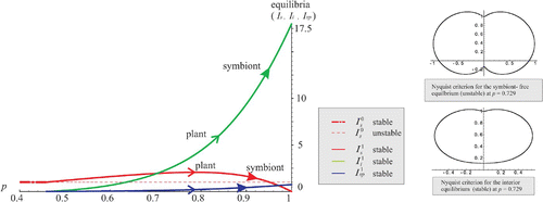
A relatively small increase in the susceptible plants mortality and in the infected plants fertility may change Case 4 into Case 5 (Figure 5). The symbiont-free equilibrium is stable for p ≤ p ₁=0.787, but for larger values of p it loses the stability and two interior equilibria emerge: , unstable on (p ₁, p ₂) and , stable on (p ₁, 1). Both plant and symbiont evolution drive p to value 1, where the metapopulation becomes 100% infected.

Figure 5. The symbiont-free equilibrium stable on (0, 0.787). One unstable interior equilibrium on (0.7659,0.787), one stable interior equilibrium on (0.7659, 1). Arrows indicate evolution of p as strategy of the plant or symbiont.

6. Conclusions

We have previously designed a model for exclusively vertically transmitted symbionts in a plant metapopulation 20 31, which we extend in this paper by allowing mixed reproduction strategies for the symbiont. Several new interesting developments have occurred throughout this work.

• First, a slight shift in the point of view of a newborn individual, which is now considered as an established plant, is ready to produce seeds itself, instead of the newly produced seeds we dealt with previously. We talk now of a renewal state rather than birth state.

• Second, the proportion p of infected seeds produced by one infected plant, which accounts for the success of the vertical transmission, is either a trait of the infected plant, or of the symbiont hosted by the plant. As a consequence of the horizontal transmission, the fitness of the plant (dominant eigenvalue of the next generation matrix) and the fitness of the symbiont (expected number of new infected plants produced by one infected plant) are different.

• Moreover, the selection gradient may differ as well. There are situations when the interests of the mutant plant and of the mutant symbiont are aligned. In other situations, as illustrated by several examples in Section 4, while the symbiont selection pressure will always increase p towards value 1, the plant evolution drives p to lower values. Hence, there is the conflict between the plant and the symbiont.

Our previous results in 20 show that the symbiont cannot persist in a qualitatively uniform environment (identical patches), if it has negative effect on the host fitness. It does, however, persist if it is mutualistic, increasing the plant fitness, or neutral, having no effect whatsoever on the host fitness

If the symbiont has mixed reproduction strategy the situation is not as black and white as before. The symbiont can invade a susceptible metapopulation either by seeds or by spores. At equilibrium, coexistence is possible whether the symbiont is mutualistic or not. It may decrease fertility or increase mortality of the host, thus lowering the host fitness, and still be able to persist in the metapopulation due to its horizontal spreading. In fact, as pointed out by the second example in Section 4, the ability to spread horizontally may be critical, as it is the only means to avoid extinction.

However, one cannot say for sure how the plant–symbiont association will evolve. In situations of conflict, as in Examples 2, 4 and 5, the plant may succeed in reducing the vertical reproductive success of the symbiont, which in return would evolve towards parasitism; on the contrary, the symbiont could reach the maximum vertical reproductive success and infect the metapopulation 100% (Example 4) or, at least, escape extinction (Example 2). The question of the evolutionarily outcome in this conflictual situations remains open. The phenotype p that we can observe in a metapopulation is probably a function of two different phenotypes: one for the plant host, and one for the symbiont. One could model mechanistically the plant–symbiont interaction and study the coevolutionary dynamics of the host and symbiont in order to obtain more specific results.

As we have pointed out, the metapopulation structure is given solely by the presence of the local catastrophes. In the absence of the catastrophes we deal with one single well mixed population. Due to the horizontal spreading of the symbionts, the dynamics of a single population still exhibits rich behaviour, similar to the metapopulation case. One could then argue that the model could be reduced to a simpler one with a single patch. Even in a single patch model symbionts are able to persist at equilibrium. However, there are cases when they would not be able to invade in a symbiont-free population. In these cases the fragmentation of the habitat would create proper condition for the symbiont invasion, followed by fixation of the metapopulation at a stable coexistence equilibrium. Moreover, the metapopulation model developed in this paper provides a basis for further investigation of heterogenous metapopulations with different local conditions from patch to patch.

References

- Allen , M. F. 1991 . The Ecology of Mycorrhizae , New York : Cambridge University Press .
- Breen , J. P. 1994 . Acremonium endophyte interactions with enhanced plant resistance to insects . Annu. Rev. Entomol. , 39 : 401 – 423 .
- Chet , I. 1993 . Biotechnology in Plant Disease Control , New-York : Wiley-Liss .
- Clay , K. 1990 . Fungal endophytes of grasses . Annu. Rev. Ecol. Systemat. , 21 : 275 – 297 .
- Clay , K. and Holah , J. 1999 . Fungal endophytes symbiosis and plant diversity in successional . Science , 285 : 1742 – 1744 .
- Denison , R. F. and Kiers , E. T. 2004 . Lifestyle alternatives for rhizobia: mutualism, parasitism and forgoing symbiosis . FEMS Microbiol. Lett. , 237 ( 2 ) : 187 – 193 .
- Denison , R. F. and Kiers , E. T. 2004 . Why are most rhizobia beneficial for their plant hosts, rather than parasitic? . Microbes Infect. , 6 ( 13 ) : 1235 – 1239 .
- Diekmann , O. and Gyllenberg , M. 2007 . “ Abstract delay equations inspired by population dynamics ” . In Functional analysis and Evolution Equations , Edited by: Amman , H. , Arendt , W. , Hieber , M. , Neubrander , F. , Nicaise , S. and von Below , J. 187 – 200 . Basel, Boston : Birkhäuser .
- Diekmann , O. , Getto , Ph. and Gyllenberg , M. 2007 . Stability analysis of Volterra functional equations in the light of suns and stars . SIAM J. Math. Anal. , 39 : 1023 – 1069 .
- Diekmann , O. , Gyllenberg , M. and Metz , J. A.J. 2003 . Steady state analysis of structured population models . Theor. Popul. Biol. , 63 : 309 – 338 .
- Diekmann , O. , Gyllenberg , M. , Metz , J. A.J. and Thieme , H. R. 1993 . “ The ‘cumulative’ formulation of (physiologically) structured population models ” . In Evolution Equations, Control Theory and Biomathematics , Edited by: Lumer , G. and Clement , Ph. 145 – 154 . New York : Marcel Dekker .
- Diekmann , O. , Gyllenberg , M. , Metz , J. A.J. and Thieme , H. R. 1998 . On the formulation and analysis of general deterministic structured population models. I. Linear theory . J. Math. Biol. , 36 : 349 – 388 .
- Diekmann , O. , Gyllenberg , M. , Metz , J. A.J. and Thieme , H. R. 2001 . On the formulation and analysis of general deterministic structured population models. II. Nonlinear theory . J. Math. Biol. , 43 : 157 – 189 .
- Ewald , P. W. 1987 . Transmission modes and evolution of the parasitism-mutualism continuum . Ann. N. Y. Acad. Sci. , 503 : 295 – 306 .
- P. E.M. 1975 . Fine, Vectors and vertical transmission: an epidemiologic perspective . Ann. N. Y. Acad. Sci. , 266 : 173 – 194 .
- Gyllenberg , M. and Hanski , I. 1992 . Single-species metapopulation dynamics: A structured model . Theor. Popul. Biol. , 42 : 35 – 62 .
- Gyllenberg , M. and Metz , J. A.J. 2001 . On fitness in structured metapopulations . J. Math. Biol. , 43 : 545 – 560 .
- Gyllenberg , M. , Hanski , I. and Hastings , A. 1997 . “ Structured metapopulation models ” . In Metapopulation Dynamics: Ecology, genetics and evolution , Edited by: Gilpin , M. and Hanski , I. 93 – 122 . London : Academic Press .
- Gyllenberg , M. , Hanski , I. and Metz , J. A.J. 2004 . “ Spatial dimensions of population viability ” . In Evolutionary Conservation Biology , Edited by: Couvet , D. , Ferrire , R. and Dieckmann , U. 59 – 80 . New York : Cambridge University Press .
- Gyllenberg , M. , Preoteasa , D. and Saikkonen , K. 2002 . Vertically transmitted symbionts in structured host metapopulations . Bull. Math. Biol. , 64 : 959 – 978 .
- Hanski , I. 1999 . Metapopulation ecology , Oxford, New York : Oxford Series in Ecology and Evolution .
- Hanski , I. and Gilpin , M. E. 1997 . Metapopulation biology: Ecology, Genetics and Evolution , San Diego, CA : Academic Press .
- Herre , E. A. 1993 . Population structure and evolution of virulence in nematode parasites of fig wasps . Science , 259 : 1442 – 1445 .
- Hoveland , C. S. 1993 . Importance of economic significance of the acremonium endophytes: a continuum of interactions with host plants . Agri. Ecosyst. Environ. , 44 : 3 – 12 .
- Lipsitch , M. , Sillerand , S. and Nowak , A. 1996 . The evolution of virulence in pathogens with vertical and horizontal transmission . Evolution , 50 : 1729 – 1741 .
- Lipsitch , M. , Nowak , A. , Ebert , D. and May , R. 1995 . The population dynamics of vertically and horizontally transmitted parasites . Proc. Roy. Soc. Lond. B. Biol. Sci. , 260 : 321 – 327 .
- Metz , J. A.J. and Gyllenberg , M. 2001 . How should we define fitness in structured metapopulation models? including an application to the calculation of evolutionarily stable dispersal strategies . Proc. Roy. Soc. Lond. B. , 268 : 499 – 508 .
- Nadkarni , N. M. , Merwin , M. C. and Nieder , J. 2001 . “ Forest canopies: plant diversity ” . In Encyclopedia of Biodiversity , Edited by: Levin , S. 27 – 40 . San Diego, , California, USA : Academic Press .
- D. Preoteasa, Ph.D. diss., University of Helsinki, (in preparation).
- Saikkonen , K. 2000 . Kentucky-31, far from home . Science , 287 : 1887a
- Saikkonen , K. , Ion , D. and Gyllenberg , M. 2002 . The persistence of fungal endophytes in grass metapopulations . Proc. Roy. Soc. Lond. B. , 269 : 1397 – 1403 .
- Saikkonen , K. , Faeth , S. H. , Helander , M. and Sullivan , T. J. 1998 . Fungal endophytes: a continuum of interactions with host plants . Annu. Rev. Ecol. Systemat. , 29 : 319 – 343 .
- Snäll , T. , Ehrlém , J. and Rydin , H. 2005 . Colonisation-extinction dynamics of an epiphyte metapopulation in a dynamic landscape . Ecology , 86 : 106 – 115 .
- Wilkinson , D. M. and Sherratt , T. N. 2001 . Horizontally acquired mutualisms, an unsolved problem in ecology? . Oikos , 92 : 377 – 384 .