Dynamics of an HIV-1 therapy model of fighting a virus with another virus

Abstract

In this paper, we rigorously analyse an ordinary differential equation system that models fighting the HIV-1 virus with a genetically modified virus. We show that when the basic reproduction ratio ℛ₀<1, then the infection-free equilibrium E ₀ is globally asymptotically stable; when ℛ₀>1, E ₀ loses its stability and there is the single-infection equilibrium E _s. If ℛ₀∈(1, 1+δ) where δ is a positive constant explicitly depending on system parameters, then the single-infection equilibrium E _s that is globally asymptotically stable, while when ℛ₀>1+δ, E _s becomes unstable and the double-infection equilibrium E _d comes into existence. When ℛ₀ is slightly larger than 1+δ, E _d is stable and it loses its stability via Hopf bifurcation when ℛ₀ is further increased in some ways. Through a numerical example and by applying a normal form theory, we demonstrate how to determine the bifurcation direction and stability, as well as the estimates of the amplitudes and the periods of the bifurcated periodic solutions. We also perform numerical simulations which agree with the theoretical results. The approaches we use here are a combination of analysis of characteristic equations, fluctuation lemma, Lyapunov function and normal form theory.

Keywords:

• HIV-1 dynamics
• recombinant virus
• stability
• Lyapunov function
• LaSalle invariance principle
• fluctuation lemma

AMS Subject Classification :

• 34K25
• 34K60
• 92B05
• 92D30

1. Introduction

In recent years, mathematical modelling has contributed greatly to the understanding of HIV-1 infection in host and has provided valuable insight into HIV-1 pathogenesis. Among various models is the class by differential equations, which quantitatively describe the dynamics of the HIV-1 virus, healthy and infected cells and even possibly the immune responses. By studying these models, researchers have gained much knowledge about the mechanism of the interactions of these components within a host, and have thereby enhanced the progress in understanding the HIV-1 infection (see, e.g. 14–17). Such understanding in turn may offer guidance for developing new drugs and for designing optimal combination of existing therapies (see, e.g. 6 10 18 and the references therein).

A standard and classic differential equation model for HIV infection is the following system of ordinary differential equations (ODEs) (see, e.g. 10 14 16):

where x(t), y(t) and v(t) are the densities of uninfected target cells, infected target cells and the free virus, respectively, at time t. Here a mass action infection mechanism is adopted, with an infection rate constant β. The healthy cell is assumed to be produced at a constant rate λ. It is also assumed that once cells are infected, they may die at rate a either due to the action of the virus or the immune system, and in the mean time, they each produces HIV-1 virus particles at a rate k during their life which on average has length 1/a.

It is known that the HIV-1 virus load is a crucial measurement of the severity of an HIV-1 carrier. When the load exceeds certain level after a clinically latent phase, the CD ⁺ T-cell count declines drastically, indicating a transition from HIV to AIDS (see, e.g. 5 20). Most of the existing therapies for HIV and/or AIDS employ inhibitors of the enzymes required for replication of HIV-1 virus to reduce the load (see, e.g. 3 8). Recent progress in genetic engineering has offered an alternative approach: modification of a viral genome can produce recombinants capable of controlling infections by other virus. Indeed, this method had been used to modify rhabdovirus, including the rabies and the vesicular stomatitis, making them capable of infecting and killing cells previously attacked by HIV-1 (for details, see, e.g. 9 13 19 22). To understand this approach of fighting a virus with a genetically modified virus, Revilla and Garcia-Ramos 18 proposed a mathematical model which is a result of incorporating into Equation (1) two more variables: the density w of the recombinant (genetically modified) virus and the density z of doubly infected cells.

Here it is assumed that (i) recombinant infects cells previously infected by the pathogen, turning them at rate α w y into doubly infected cells, and in the mean time, recombinants are removed at a rate q w and (ii) the doubly infected cells die at a rate of bz and release recombinants at a rate c z.

In 18, the authors only analysed the structure of the equilibria of the system (2) and performed some numerical simulations. System (2) has a dimension higher than 2, and it is well known that for systems with higher dimensions, equilibria cannot determine solutions’ long-term behaviours, and complicated dynamics (periodic solutions and even chaos) may occur which would make the system unpredictable. Therefore, theoretically determining the global dynamics of Equation (2) is an important yet challenging problem, and this constitutes the purpose of this paper. In Section 2, we will justify the well-posedness of the model by showing the positivity and boundedness of solutions of Equation (2) and review the existence result on equilibria and the basic reproduction number ℛ₀. In Section 3, we show that when , the disease-free equilibrium is globally asymptotically stable, and when it is unstable. In Section 4, we prove that there is a δ>0 depending on all parameters except for λ, such that if , then the single-infection equilibrium exists and is globally asymptotically stable, and when , this equilibrium loses its stability. Note that is also the condition for the existence of double-infection equilibrium. In Section 5, we analyse the stability of the double-infection equilibrium E _d and prove that when ℛ₀ is slightly larger than 1+δ, solutions of the model converge to the E _d; but when ℛ₀ is further increased in some way, E _d loses its stability via Hopf bifurcation, giving rise to stable periodic solutions. This theoretical result confirms what we stated earlier: equilibria cannot fully determine the solution dynamics, and stability analysis is important and indeed necessary. Through a numerical example, we illustrate in Section 6 how to obtain more information about the Hopf bifurcation, including the bifurcation direction, the stability, amplitude and frequency of the bifurcated periodic solution. Such information is crucial for giving good estimates of the virus load and healthy cells’ density in the case that these quantities are periodic in time variable t (i.e. sustained fluctuations), based on which, a therapy is usually determined. It may also provide guidance for designing a optimal clinical sampling strategy, such as the best time intervals of sampling. The approaches we used here are a combination of analysis of characteristic equations, fluctuation lemma, Lyapunov function and normal form theory. Our numerical simulations agree with the theoretical results. In the last section, we summarize the main results and discuss possible modifications of the model.

2. Well-posedness, equilibria and basic reproduction numbers

Since the variables are densities which cannot be negative, one expects that starting from non-negative initial values, the corresponding solution remains non-negative. This can be easily confirmed as below. First, from the first equation of Equation (2), we have

implying x(t)>0 for t>0 provided that x(0)≥0. In a similar way, one can establish non-negativity of the other four variables for t>0 provided that y(0)≥0, and w(0)≥0. Moreover, if in addition, y(0)>0 (or z(0)>0 or v(0)>0 or w(0)>0), then y(t)>0 (or z(t)>0 or v(t)>0 or w(t)>0) for t>0.

Solutions to Equation (2) also remain bounded. To see this, let be a non-negative solution. Choose and , and let

Then

This implies that every component of (x, y, z, v, w) must be bounded. By the extension theory of ODEs, the boundedness of a solution also implies that it exists for all t≥0.

Model system (2) always has the infection-free equilibrium . The other two possible biologically meaningful equilibria are

with the former being the singly infected equilibrium and the latter being the doubly infected equilibrium. From the biological meaning of the basic reproduction numbers, Revilla and Garcia-Ramos 18 identified ℛ₀ as

Applying the general mathematical theory of basic reproduction numbers for disease model described by ODEs (see, e.g. 21), we can easily confirm the above formula. It turns out that the value of ℛ₀ determines the existence of the single-infection equilibrium: E _s exists if and only if .

The double-infection equilibrium exists (biologically meaningful) if and only if Q>0 where

Introducing the second basic reproduction number

for the doubly infected cells, one can easily verify that

and hence

For convenience, we denote

With the above identities, E _s and E _d can be expressed by the following simpler formulas:

In order to analyse local stability of Equation (2) at an equilibrium E, we need to calculate the the Jacobian matrix of Equation (2) at as below:

The characteristic equation of Equation (2) at E is , whose roots determine the local stability of E.

3. Stability of the infection-free equilibrium

For the infection-free equilibrium E=E ₀, some fundamental calculations give the corresponding characteristic equation

The stability of E ₀ is determined by the sign of real parts of the roots of Equation (4): if all roots of Equation (4) have negative real parts, then E ₀ is asymptotically stable; if there is at least one root of Equation (4) has positive real part, then E ₀ is unstable. Obviously, it suffices to consider the quadratic equation

Using the Decarte's rule of sign, we know that whether or not the two roots of Equation (5) have negative real part is determined by the sign of : the negativity (positivity) of the real parts of the two root of Equation (5) is equivalent to (), that is, ().

Indeed, by employing the fluctuation lemma (see, e.g. 4), we can prove the global asymptotic stability of the infection-free equilibrium E ₀ under the condition . For this purpose, we first introduce some basic notations. For a continuous and bounded function , let

In Section 2, we have shown that for any initial values , the corresponding solution remains non-negative and is bounded from above. Therefore, the and exist for all these five component functions. By the fluctuation lemma (see, e.g. 4), there exists a sequence t _n with as n→∞ such that

From the first equation of Equation (2), we obtain

Letting n→∞ in the above equation leads to the following estimate

Similar treatment to the rest of the equations in Equation (2) gives

We claim that y ^∞=0. Otherwise, v ^∞>0 by Equation (8). From Equations (7), (8) and (10), it follows that

leading to

This contradicts to the condition . Hence, y ^∞=0 which also implies by Equations (7)–(9). Now, by the relation , we then conclude that y(t)→0 as t→∞. Similarly, z(t), v(t) and w(t) all approach 0 as t→∞. Finally, with v(t)→0, the first equation in Equation (2) becomes an asymptotically autonomous equation with the limiting equation being By the theory for the asymptotically autonomous systems (see, e.g. 1), we know that the function as t→∞. The local stability of E ₀ established in Section 2 under the assumption and the global attractivity of E ₀ established above give the global asymptotical stability of E ₀.

Summarizing the above results, we have proved the following theorem.

Theorem 3.1

When the infection-free equilibrium E ₀ is globally asymptotically stable implying the virus cannot invade regardless of initial load; when becomes unstable implying that virus may persist.

4. Stability of the single-infection equilibrium

From Section 3, we know that when ℛ₀ increases to pass the value 1, the disease-free equilibrium loses its stability and the single-infection equilibrium E _s comes into existence. In this section, we study the stability of E _s.

For the local stability of E _s, the characteristic equation of the linearized system of the model (2) at E _s is given by

where

Equation (12) may be rewritten as

Thus, the eigenvalues of Equation (12) are determined by the following two equations:

and

Equation (14) is a cubic equation of the form

The Routh–Hurwitz theorem (see 2) for this equation states that all roots have negative real parts if and only if b ₂>0, b ₀>0 and . Now, for Equation (14),

It is also easy to verify that . Hence, all roots of the cubic equation (14) have negative real parts.

For the quadratic equation (13), by a similar argument to that for Equation (5), we know that the two roots of Equation (13) have negative real parts if and only if

The first inequality holds automatically (since b>0 and q>0) and the second one is equivalent to (or Q<0). Consequently, the single-infected equilibrium E _s exists if and only if , and is locally stable if and only if (or Q<0).

Indeed, by constructing a Lyapunov function and applying the LaSalle's invariance principle, we can show that when and is globally asymptotically stable. To this end and for convenience for notation, denote by and v _s the three positive components of the single-infection equilibrium E _s, that is, and . Define

for . By calculus of multi-variable functions, it can be easily seen that has a global minimum attained at E _s and thus, and if and only . Making use of the equilibrium equation at E _s, the derivative of V along positive solutions of Equation (2) can be estimated as

It is straightforward to verify that the condition (or Q<0) is equivalent to

Thus, when , and V′=0 if and only if . By the LaSalle's invariance principle 7, we conclude that E _s is indeed globally asymptotically stable.

Summarizing the above analysis, we have established the following theorem.

Theorem 4.1

When and (equivalently Q<0 or Equation (17) holds) hold, then the single-infection equilibrium E _s is globally asymptotically stable implying that the recombinant virus cannot survive but the pathogen virus can; when becomes unstable implying that recombinant virus may persist.

5. Stability of the double-infection equilibrium E _d and Hopf bifurcation from E _d

When (equivalently Q>0 or ), the single-infection equilibrium becomes unstable and there occurs the double-infection equilibrium E _d. Unlike for E ₀ and E _s at which the characteristic equations can be factored into product of lower degree polynomials, we are unable to factor the characteristic equation at E _d, and thus cannot determine the stability of E _d by the same way as in Sections 3 and 4. On the other hand, our preliminary simulations show that for certain parameter values satisfying , solutions of Equation (2) converge to E _d, while for other parameter values the solutions of Equation (2) do not converge to E _d; instead they converge to a periodic solution. This observation shows the necessity and importance of some theoretical analyses on the stability of E _d as well as on possible Hopf bifurcation.

For convenience in the following analysis, we first do the following rescalings to reduce the number of parameters:

where

By the above, system (2) is transformed to

Under Equations (18)–(20), the basic reproduction number ℛ₀ now becomes

and the critical value of ℛ₀ for the double-infection equilibrium E _d of Equation (2) to exist becomes

In the rest of this section, we assume . Thus, the double-infection equilibrium E _d for Equation (21) exists and is now (by Equations (18)–(20)) given by

In order to examine the stability of E _d for Equation (21), we compute the Jacobian matrix of system (21) as

By straightforward but tedious computations, the characteristic polynomial of J at E _d is obtained as follows:

where

It is obvious that a ₁>0 and a ₂>0 for any positive parameter values. Here we apply the Routh–Hurwitz criterion to find the stability of the equilibrium solution E _d. The necessary and sufficient conditions for E _d to be stable are given by

where

It is easy to see that , since R ₁>1 and we have assumed . Now, we need to check the signs of . First, a straightforward calculation shows that

indicating that Δ₂>0 for all positive parameter values.

For Δ₃ and Δ₄, the signs are not easy to determine for general ℛ₀, and hence we use a continuity argument below. At , using Equation (27) and by direct calculations, we have

and

Note that and Δ₅ depend continuously on ℛ₀. From Equations (27), (29)–(32) and the continuity, we know R ₂>R ₁ such that Equation (28) holds when , leading to the following conclusion.

Theorem 5.1

There is an R ₂>R ₁ such that when the double-infection equilibrium E _d is asymptotically stable.

When ℛ₀ is further increased, Δ₁ and Δ₂ remain positive, but Δ₃ and Δ₄ may become negative (so may Δ₅ by Equation (29) and a ₅>0 as ). The following lemma identifies the order of possible sign switches for Δ₃ and Δ₄.

Lemma 5.1

If Δ₃ and Δ₄ can change signs from positive to negative as ℛ₀ is further increased after the value R ₂ in Theorem 5.1, then Δ₄ will change before Δ₃ does.

Proof

Assume, for the sake of contradiction, that Δ₃ will change sign no later than Δ₄ does. Then there exists an R ₃>R ₂ such that

Then, at ,

from which we obtain

Thus,

leading to a contradiction to . This completes the proof.   ▪

The following lemma tells that when Δ₄ crosses zero, Δ₃ must remain positive.

Lemma 5.2

For any if Δ₄=0, then Δ₃>0.

Proof

Suppose Δ₄=0 at . Then,

and hence

On the other hand, the third equation in Equation (29) leads to

Subtracting Equation (35) from Equation (34) results in

Note that a ₅>0 and Δ₂>0. Also, a careful calculation gives

which clearly shows that when . This together with Equation (36) confirms Δ₃>0, completing the proof.   ▪

The above discussion and the results in Yu 24 imply that there are no static bifurcation, Hopf-zero bifurcation, double Hopf bifurcation and double-zero Hopf bifurcation, emerging from the equilibrium solution E _d; and the only possibility for E _d to lose stability is occurrence of Hopf bifurcation when Δ₄ crosses zero from positive to negative as ℛ₀ further increases from R ₂ (see Theorem 5.1).

In order to show that Hopf bifurcation can occur, we need to show that Δ₄ can change sign from positive to negative as ℛ₀ further increases after R ₁. To this end, we notice that and , implying that as while remains valid (actually, as long as 1/a>dp+bq/c). The above observation suggests considering small values of a and large values of c. Indeed, by Equations (27), (29) and tedious but straightforward expansion, we may obtain

where

in which

Thus, for small a and large c, the sign of Δ₄ is determined by the leading coefficient c ₄, i.e. the sign of f(d). In order to have c ₄>0, we need f(d)>0, which holds for appropriate values of d. For example, f(d)>0 when d<d ₁ or d>d ₂ where d ₁ and d ₂ are the two roots of f(d)= as a quadratic function of d:

Combining the above and the results in Yu 24, we have proved the following theorem.

Theorem 5.2

For some large values of c and small values of a, together with d<d ₁ or d>d ₂ (d ₁, d ₂ as given in Equation (40)) (hence the double-infection equilibrium E _d loses its stability through Hopf bifurcation, giving rise to a family of periodic solutions.

By the above theorem, E _d can lose its stability through Hopf bifurcation when ℛ₀ is further increased from R ₁ in some way. It should be pointed out that the conditions obtained above for Δ₄ to change sign (i.e. for large values of c and small values of a) are only sufficient conditions for the requirement , which may be quite conservative. There may be many other choices of the parameters that can satisfy this requirement. For some special choice, we may even find the critical value R _h for ℛ₀ precisely at which Hopf bifurcation occurs. This will be illustrated numerically in the following section.

6. Numerical illustrations

In this section, we use a numerical example and some simulations to demonstrate the theoretical results obtained in the previous sections. Due to the larger number of parameters, there are many choices for this purpose. For convenience, we will work on the scaled model (21) instead of the original model (2). Throughout this section, we fix

but choose d as the bifurcation parameter. Then,

The infection-free equilibrium becomes

which is stable when (i.e. ). When d decreases to pass the critical value increases to pass the threshold value 1, and E ₀ becomes unstable and there occurs the single-infection equilibrium

which is stable for (corresponding to ). When d further decreases to pass the critical value increases to pass R ₁ and E _s loses its stability to the double-infection equilibrium

which is stable when

where d _h or R _h is determined as follows.

For the given parameter values, the coefficients of the characteristic polynomial for E _d become

and thus

A numerical scheme for solving the roots of polynomial can be applied here to find three positive real solutions of Δ₄=0, given by

It is seen that only the first solution satisfies the requirement, and thus

giving a corresponding value

for ℛ₀ by the formula of ℛ₀ in Equation (42) in terms of d. Hence, when

the equilibrium solution E _d is stable. At the critical point, , the equilibrium solution E _d becomes unstable and a Hopf bifurcation occurs, leading to a family of periodic solutions. In fact, at the critical point , other Routh–Hurwitz conditions are satisfied as

Indeed, with these given parameter values, one can numerically find the eigenvalues of the characteristic polynomial P _d (ξ) which include a pair of pure imaginary roots and three negative real roots:

where i is the imaginary unit, i ²=−1.

In what follows, we show, via this numerical example, how to obtain more information about the Hopf bifurcation, such as bifurcation direction and stability, magnitudes and periods of the bifurcated period solutions. To this end, we apply the normal form theory and the program using computer algebra system Maple developed by Yu 23, and Yu and Huseyin 25 to analyse the Hopf bifurcation of system (21) from the critical point (with other parameters given by Equation (41)).

The general normal form can be written in polar coordinates as

where r and θ represent the amplitude and phase of periodic motion (limit cycle), respectively. The constant corresponds to the pair of the pure imaginary roots of are constants, depending on the original system parameters, with v ₀ and v ₁ being called focus values (or Lyapunov coefficients). When , the Hopf bifurcation is supercritical (subcritival), giving stable (unstable) limit cycles, and the periodic solutions can be approximated in terms of the steady-state solution of Equation (45) (see 23 for details). v ₀ and τ₀ can be found from linear analysis, while v ₁ and τ₁ must be determined by using nonlinear analysis. We show how to find these constants below for this numerical example.

Let , where μ is small perturbation (bifurcation) parameter, and

By the linear transformation

system (21) is transformed to

in which

Here o (μ) denotes a term containing only higher orders of μ. Now, the Jacobian of system (47) evaluated at the trivial equilibrium solution (corresponding to E _d for Equation (21)) is in the Jordan canonical form:

By Yu and Huseyin 25, the coefficients v ₀ and τ₀ are given by

Applying the Maple program developed in Yu 24 to system (47) (setting μ=0) results in

Therefore, the third-order normal form Equation (45) becomes

The steady-state solutions of Equation (51) are determined by setting , yielding

The solution r¯=0 actually corresponds to the equilibrium solution E _d of Equation (21). A simple linearization of the first equation of Equation (51) indicates that ) is stable for μ<0, as expected. When μ increases from negative to cross zero, a Hopf bifurcation occurs and the amplitude of the bifurcation periodic solutions is given by the non-zero steady-state solution

Since v ₁<0, the Hopf bifurcation is supercritical and the bifurcating limit cycle is stable. The amplitude of the bifurcating limit cycle is given by Equation (53), and the frequency is determined from the following equation:

We have performed some numerical simulations for Equation (21) by using a fourth-order Runge–Kutta method. We take the parameter values given in Equation (41), giving and . We choose four different values for d (and so for ℛ₀ ):

According to the above theoretical analysis, the simulation results are expected to have the stable equilibrium solution E ₀ for d=0.21, the stable equilibrium solution E _s for d=0.10, the stable equilibrium solution E _d for d=0.04 and a stable limit cycle for d=0.022 (for which ), with approximate amplitude for the periodic motion, .

The simulated time history and phase portraits for the above four cases are shown in Figures 1 – 4, respectively, where the initial conditions are taken as

It can be seen from these figures that the numerical simulation results agree with the analytical predictions. The solutions for the first three cases converge to the equilibrium points, E ₀, E _s and E _d, respectively. For the last case, the simulated amplitude of the limit cycle (see Figure 4) is close to the predicted value, , showing a good agreement, not only qualitatively, but also quantitatively, between the theoretical prediction and numerical simulation. Also, it is seen that the period of motion, (ω is given in Equation (54)), decreases as μ increases. In other words, T decreases as d decreases. However, since μ is quite small, the change of the period due to μ is not significant (hardly observed, see Figures 4 and 5). Nevertheless, a small change in μ can cause large variation of the amplitude. The simulation results shown in Figure 5 uses d=0.012, which gives and thus the approximation of the amplitude of periodic motion is , which is almost 2.3 times of that when d=0.022. This can be observed from Figures 4b and 5b.

Figure 1. Simulated time history of system (21) for d=0.21, a=0.93, c=40, b=p=q=5.6 with the initial condition: x(0)=5.0, y(0)=1.0, z(0)=2.0, v(0)=0.5, w(0)=4.0, converging to the stable equilibrium solution E ₀.

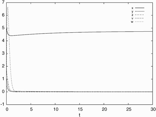
Figure 2. Simulated time history of system (21) for d=0.10, a=0.93, c=40, b=p=q=5.6 with the initial condition: x(0)=5.0, y(0)=1.0, z(0)=2.0, v(0)=0.5, w(0)=4.0, converging to the stable equilibrium solution E _s.

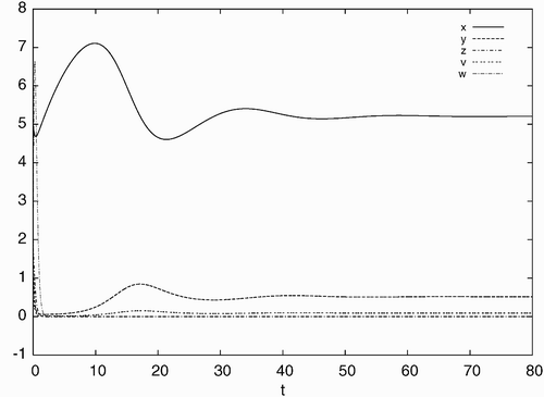
Figure 3. Simulated time history of system (21) for d=0.04, a=0.93, c=40, b=p=q=5.6 with the initial condition: x(0)=5.0, y(0)=1.0, z(0)=2.0, v(0)=0.5, w(0)=4.0, converging to the stable equilibrium solution E _d.

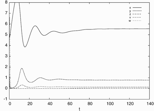
Figure 4. Simulation results of system (21) for d=0.022, a=0.93, c=40, b=p=q=5.6 with the initial condition, x(0)=5.0, y(0)=1.0, z(0)=2.0, v(0)=0.5, w(0)=4.0: (a) time history showing convergence to a stable periodic solution and (b) phase portrait projected on x−y plane indicating a stable limit cycle.

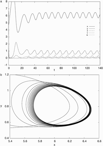
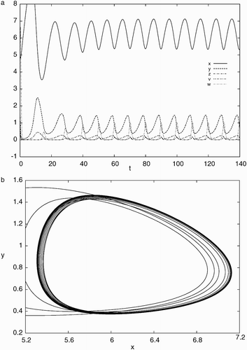
Figure 5. Simulation results of system (21) for d=0.012, a=0.93, c=40, b=p=q=5.6 with the initial condition, x(0)=5.0, y(0)=1.0, z(0)=2.0, v(0)=0.5, w(0)=4.0: (a) time history showing convergence to a stable periodic solution and (b) phase portrait projected on x−y plane indicating a stable limit cycle.

7. Conclusion and discussion

Revilla and Garcia-Ramos 18 proposed a model to describe the interaction of HIV-1 virus, a genetically modified virus, healthy T-cells and infected T-cells, and in terms of theory, they only analysed the structure of the equilibria of the model. As we emphasized in Section 1, for a higher-dimensional system, its dynamics cannot be fully determined by the structure of equilibria, and stability analysis is crucial and necessary. In this paper, we have fully analysed the stability of the infection-free equilibrium E ₀, the single-infection equilibrium E _s and the double-infection equilibrium E _d and theoretically proved following:

1. when , the disease-free equilibrium E ₀ is globally asymptotically stable;

2. when , E ₀ becomes unstable and there occurs the single-infection equilibrium E _s.

3. when , E _s is globally asymptotically stable;

4. when (equivalently ), E _s becomes unstable, and there is the double-infection equilibrium E _d;

5. there is a , such that E _d is asymptotically stable when ;

6. when ℛ₀ is further increased in some appropriate ways, E _d loses it stability, giving rise to some stable periodic solution via Hopf bifurcation.

The above descriptions reveal the role that each parameter plays in determining the global dynamics of the model and give some quantitative criteria in terms of the parameters for controlling the infection.

Note that Equation (2) is a result of incorporating the variables z and w (recombinant related) into Equation (1). It can be easily seen that both Equations (1) and (2) share the same basic reproduction number ℛ₀, and hence the parameters in z and w equations have no impact on ℛ₀. In this sense, introducing the recombinant into to the host does not help completely eliminate the HIV virus. However, by comparing the healthy CD4⁺ T-cell populations and the wild HIV virus loads in the single-infection equilibrium and the double-infection equilibrium , we can see that the recombinant can increase the healthy cell populations and reduce the virus load. To see this, assume . Then large c and small k will guarantee that ℛ₀ is slightly large than , so that the double-infection equilibrium is asymptotically stable. Now simple calculations show the condition implies (is indeed equivalent to)

There have been various models for HIV drug therapies. Comparing the model (2) for the generic therapy with existing models for drug therapies, one finds that the latter is much simpler, because they are usually the result of replacing a parameter by another one reflecting the drug efficacy. For example, in considering the effectiveness of a reverse transcriptase inhibitor, the usual way is to replace the parameter β in Equation (1) by (see, e.g. 16), leading to

where η accounts for the drug efficacy. Clearly, Equation (58) has the same structure as Equation (1), and hence, demonstrate the same threshold dynamics as Equation (1), but now in terms of the new basic reproduction number . Obviously, positive η _rt reduces ℛ₀, implying that an effective drug may help eliminate the HIV virus. This is in contrast to the generic therapy that Equation (2) models (see the above paragraph).

We point out that 18 only numerically explored solution behaviour of model (2). Now after some rigorous analysis, we have obtained conditions in terms of the model parameters on the stability of the equilibria and E _d, given by the descriptions (1)–(5) above. Moreover, the description (4) above (or Theorem 5.2) identifies an important class of solutions: periodic solutions. Considering the fact that the sustained fluctuation of the virus load and/or the healthy cells’ population in vivo will make the clinic measurements of these two quantities less reliable, this finding is of particular theoretical and practical significance. For example, without excluding the period dynamics, a very lower load of virus in the clinic sampling may right be the value of a periodic solution at the lowest moment and hence does not imply that virus is dying out. In order to avoid misleading and to make good use of clinical data in such a periodic situation, information about the frequencies and magnitudes of the oscillating densities is necessary. Through a numerical example, we have demonstrated how to obtain such information. Knowledge on the periods of oscillation of solutions may help design optimal clinical sampling strategy, e.g. the time interval for sampling.

The interaction of HIV virus and T-cells is a complicated process, which involves cell production, virus attachment to the cells and penetration into the cells, virus replication inside cells and release from cells. Now with a recombinant virus added in, the process becomes more complicated. The model we consider here is just a simple one, and there is more room to improve and expand the model. For example, one may consider the situation when there is an external source of recombinant virus. One may also consider the situation when the recombinant virus also infects susceptible cells but at a lower rate (this may occur due to possible mutation of the recombinant virus). One may also incorporate the infection latent into the model, as in 11 12, that leads to models of delay differential equations. Such modifications should more precisely describe the reality and give us more insights into the infection process, but would lead to much more challenging mathematical problems.

Acknowledgements

This research was supported by NSERC of Canada, PREA of Ontario and by China Scholarship Council.

References

- Castillo-Chavez , C. and Thieme , H. R. 1995 . “ Asymptotically autonomous epidemic models ” . In Mathematical Population Dynamics: Analysis of Heterogeneity, I. Theory of Epidemics , Edited by: Arino , O. 33 – 50 . Canada : Wuerz, Winnipeg .
- Gantmacher , F. R. 1959 . The Theory of Matrices , Vol. 2 , New York : Chelsea .
- Haase , A. T. 1999 . Population biology of HIV-1 infection: virus and CD+ 4 T cell demography and dynamics in lymphatic tissues . Ann. Rev. Immunol. , 17 : 625 – 656 .
- Hirsch , W. M. , Hanisch , H. and Gabriel , J.-P. 1985 . Differential equation models of some parasitic infections: methods for the study of asymptotic behaviour . Comm. Pure Appl. Math. , 38 : 733 – 753 .
- Janeway , C. and Travers , P. 2005 . Immunobiology: The Immune System in health and Disease , New York : Garland .
- Kepler , T. and Perelson , A. 1998 . Drug concentration heterogeneity facilitates the evolution of drug resistance . Proc. Natl. Acad. Sci. USA , 95 : 11514 – 11519 .
- LaSalle , J. P. 1976 . The Stability of Dynamics Systems , Philadelphia : SIAM .
- Levy , J. 1998 . HIV and the Pathogenesis of AIDS , Washington, DC : AMS .
- Mebatsion , T. , Finke , S. , Weiland , F. and Conzelmann , K. 1997 . A CXCR4/CD4 pseudotype rhabdovirus that selectively infects HIV-1 envelope protein-expressing cells . Cell , 90 : 841 – 847 .
- Nelson , P. , Mittler , J. and Perelson , A. 2001 . Effect of drug efficacy and the eclipse phase of the viral life cycle on estimates of HIV-1 viral dynamic parameters . J. Acquir. Immune. Defic. Syndr. , 26 : 405 – 412 .
- Nelson , P. , Murray , J. and Perelson , A. 2000 . A model of HIV-1 pathogenesis that includes an intracellular delay . Math. Biosci. , 163 : 201 – 215 .
- Nelson , P. and Perelson , A. 2002 . Mathematical analysis of delay differential equations for HIV . Math. Biosci. , 179 : 73 – 94 .
- Nolan , G. P. 1997 . Harnessing viral devices as pharmaceuticals: fighting HIV-1s fire with fire . Cell , 90 : 821 – 824 .
- Nowak , M. and May , R. 2000 . Virus Dynamics , Oxford : Oxford University .
- Perelson , A. , Kirschner , D. and De Boer , R. 1993 . Dynamics of HIV infection of CD4 + T cells . Math. Biosci. , 114 : 81 – 125 .
- Perelson , A. and Nelson , P. 1999 . Mathematical models of HIV dynamics in vivo . SIAM Rev. , 41 : 3 – 44 .
- Perelson , A. , Neumann , A. , Markowitz , M. , Leonard , J. and Ho , D. 1996 . HIV-1 dynamics in vivo: Virion clearance rate, infected cell life-span, and viral generation time . Science , 271 : 1582 – 1586 .
- Revilla , T. and Garcia-Ramos , G. 2003 . Fighting a virus with a virus: a dynamic model for HIV-1 therapy . Math. Biosci. , 185 : 191 – 203 .
- Schnell , M. J. , Johnson , E. , Buonocore , L. and Rose , J. K. 1997 . Construction of a novel virus that targets HIV-1 infected cells and control HIV-1 infection . Cell , 90 : 849 – 857 .
- Stilianakis , N. I. and Schenzle , D. 2006 . On the intra-host dynamics of HIV-1 infections . Math. Biosci. , 199 : 1 – 25 .
- van den Driessche , P. and Watmough , J. 2002 . Reproduction numbers and sub-threshold endemic equilibria for compartmental models of disease transmission . Math. Biosci. , 180 : 29 – 48 .
- Wagner , E. K. and Hewlett , M. J. 1999 . Basic Virology , New York : Blackwell .
- Yu , P. 1988 . Computation of normal forms via a perturbation technique . J. Sound Vib. , 211 : 19 – 38 .
- Yu , P. 2005 . Closed-form conditions of bifurcation points for general differential equations . Int. J. Bifurcation Chaos Appl. Sci. Eng. , 15 : 1467 – 1483 .
- Yu , P. and Huseyin , K. 1988 . A perturbation analysis of interactive static and dynamic bifurcations . IEEE Trans. Automat. Control , 33 : 28 – 41 .