Quiescence stabilizes predator–prey relations

Abstract

The classical MacArthur Rosenzweig predator–prey system has a stable coexistence point or, if either the prey capacity is large or the predator mortality is low, a stable limit cycle. The question here is how the stability properties of the coexistence point change when the prey or the predator or both can go quiescent. It can be shown that a stable equilibrium stays stable, but an unstable equilibrium may become stable. The exact stability domain is determined. In general, increasing the duration of the quiescent phase of the prey or of the predator widens the stability window. Numerical studies show that limit cycles shrink when quiescent phases are introduced.

Keywords:

• predator–prey system
• quiescent phase
• stability domain

Mathematics Subject Classification :

• 34C11
• 34C23
• 34D23
• 92D40

1. Introduction

Since Kolmogorov's 1936 paper 12, it has been known that a two-dimensional predator–prey system may exhibit stable limit cycles. These limit cycles are biologically more relevant than the families of periodic orbits that appear in the simplest Hamiltonian Lotka–Volterra system ˙ u=u−uv, ˙ v=uv−v. While Kolmogorov showed the existence of limit cycles for a wide class of systems with certain qualitative properties, MacArthur and coworker 19, and later Rosenzweig 18 designed specific models in terms of carrying capacity and rates. In particular, the notion of a ‘paradox of enrichment’ has attracted much attention. After Hollings 10 coined the notion of functional response, the results on existence of limit cycles could be connected to specific types of biological response functions. An enormous literature exists on existence and uniqueness of such limit cycles. The problem of uniqueness has been studied with great effort, probably not for its biological relevance, but for its connection to the only unsolved Hilbert problem (the sixteenth). It is not our goal to review the existing literature on this subject, but to shed some light on predator–prey interaction for the specific example of the MacArthur–Rosenzweig model.

Quiescence plays an important role in ecology. Bacteria may go quiescent when the environment becomes unsuitable. Mammalian herbivores may be quiescent for most of the day in order to avoid predators. Predators may be quiescent when hunting is not expected to be successful. Of course for many species, quiescent periods are dictated by the annual or the diurnal cycle.

Here we study systems in which each species (or rather, its individuals) can go quiescent and return to activity at certain rates. Whereas seasonal models lead to non-autonomous differential equations, our models, based on diffusive coupling to quiescent phases, lead to autonomous systems. Such systems have been studied earlier for tumour growth, see e.g., 4 11, and then for reaction, diffusion, and transport 6 8 13, the river drift paradox 16, with rates depending on population density 14, and for meta-populations 15. The applications to ecological problems have led to systematic studies of the dynamical systems’ aspects 7 9.

Some models with diffusive coupling to a quiescent phase can be interpreted in spatial terms. Then the quiescent phase corresponds to a refuge that is inaccessible to the other species.

In a recent paper 5 (as announced in 7), it has been shown that for systems with any number of species, introducing quiescent phases, with the same entrance and exit rates for all species, stabilizes against the onset of oscillations.

This stabilizing effect is very specific, in particular, it stabilizes against Hopf bifurcations. If we consider a stationary state and the eigenvalues of the Jacobian matrix at that state, then with quiescence real eigenvalues retain their signs (zero eigenvalues stay zero), while for truly complex eigenvalues with positive real parts, the real parts are decreased and may even become negative. Hence Hopf bifurcations are less likely with quiescence. With respect to a critical parameter, the bifurcation may come ‘later’ or not at all (Figure 1). Also it has been shown, in 7, for a class of highly symmetric problems, that a quiescent phase reduces the amplitude of existing limit cycles (similar to Figure 1, right). These results apply when all species go quiescent and return with the same rates. The case of different rates for different species has been attacked in 5 for two species. A close connection to the Turing instability has been exhibited. The case of more than two species appears as untractable as the Turing problem 20.

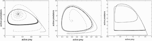
Figure 1. Three phase planes for the MacArthur–Rosenzweig system (solid) and the corresponding system with quiescence (dashed, trajectories have been projected from four dimensions onto the u, v-plane). In each case, the MR system has a limit cycle. Left (just inside the stability region): the system with quiescence has a stable stationary point. Centre (deep inside the stability region): rapid convergence to stationary point. Right (outside the stability region): both systems have limit cycles. The projected limit cycle of the quiescent system is much smaller than that of the MR system.

In the present paper, we continue to examine the case of different rates. We want to find out what happens when we have potentially oscillatory predator–prey dynamics and assume quiescent phases with different rates. The MacArthur–Rosenzweig model is perfect for this project, as many computations can be done explicitly, and the results can be discussed in terms of quantities that are established in the ecological literature. This model depends on six parameters (three after scaling), and there are four rates related to quiescence. We get a four-dimensional system, and consequently a characteristic polynomial of order four depending on many parameters in a complicated way. Nevertheless, after rewriting the Routh–Hurwitz conditions in a suitable form, we get a coherent theory. In Section 2, we present the problem and the stability theorem as well as a theorem on existence of a global attractor. These theorems are proved in Sections 3 and 4.

2. The problem and the results

In the classical formulation the MacArthur Rosenzweig model reads

Here we prefer an equivalent formulation which better shows the behaviour at low densities:

The parameter K is the carrying capacity of the prey, and a is its growth rate at low population densities. The parameter b is the consumption rate at low prey density, and c is the exploitation rate, i.e., the rate by which consumed prey is invested in population growth. The parameter m measures saturation. The parameter B is the prey density at the coexistence state. The quotient B/(1+mB) can be seen as predator mortality.

The system with quiescent phases reads

The variable w denotes the prey in the quiescent phase, while z is the predator in the quiescent phase. The p _i are the rates at which the prey and the predator, respectively, go quiescent. The q _i are the rates at which each species returns to the active state. All these rates are positive.

So we have a two-dimensional system (2) and a four-dimensional system (3) that are closely related with respect to the biological interpretation and the general form of the equations.

Also the stationary states are closely related 7. If (u, v) is a stationary state of the system without quiescence (2), then is a stationary state of the system with quiescence.

The stationary states of the system (2) are (0, 0), (K, 0), and the coexistence state which is feasible for B<K,

Here we are interested only in the stability of the coexistence state. The determinant and the trace of the Jacobian matrix are

Hence the coexistence state is stable if and only if

The following is well known 2. If B>B¯, then the coexistence state is stable, and it is globally stable in the set where u, v>0. If B<B¯, then the coexistence state is unstable, and there are limit cycles running around the coexistence point. In the specific case of the system (2) it is known that there is exactly one limit cycle that attracts all trajectories with u, v>0, except the coexistence point.

The destabilizing effect can be achieved by either decreasing B from values larger than B¯ to values lower than B¯, thus in effect by decreasing predator mortality, or by increasing the carrying capacity K of the prey. That is, it appears as if enriching the opportunities for predators by increasing the prey level destabilizes the equilibrium; hence the ‘paradox of enrichment’.

Here we describe the stability domain for the problem with quiescence. Looking at the problem from biology, one would keep the ‘physiological’ parameters of the MacArthur–Rosenzweig system fixed and vary the ‘behavioural’ parameters p _i and q _i . However, notice that the parameters K, a, b, c, B, and m enter the stability problem only via the trace τ and the determinant δ. Hence one gets a much clearer picture if one keeps the four coefficients p ₁, q ₁, p ₂, q ₂ fixed and lets only τ and δ>0 vary. The trace τ may have either sign. In a τ, δ-plane, the stability domain of the system without quiescence is exactly the quadrant τ<0, δ>0. The stability domain of the system with quiescence is described by the following theorem (Figure 2). For convenience, we introduce

Theorem 1

The stability domain of the problem with quiescence is the set

with

where is the smallest positive root τ, for given δ>0, of the cubic equation in τ

The curve starts from τ=0 and δ=0. Along the curve, δ increases to +∞. The curve is asymptotic to the line τ=p.

The domain 𝒟 can also be described in terms of the real roots , for given τ>0, of the quadratic equation (10) (Figure 2).

Hence the stability domain extends into τ>0. While the system without quiescence has a Hopf bifurcation exactly for τ=0, i.e., for B=B¯, this Hopf bifurcation is now shifted to positive values of τ, i.e., to the boundary of the stability domain in the first quadrant, see Figure 2.

Figure 2. The τ, δ-plane with the null set of the cubic F and the second and third of the linear Hurwitz conditions (dashed). Quiescence leads to an enlarged stability domain that comprises the second quadrant and also the part of the first quadrant between the δ-axis and the upper branch of the null set. Broadly speaking, this domain gets larger when p ₁, p ₂ are increased. Case 1a. p ₁=0.5, p ₂=0.35, q ₁=0.6, q ₂=0.85, p<z ₁<z ₂. The first branch runs monotonely from (0, 0) to the vertical asymptote. Case 1b. p ₁=1, p ₂=0.5, q ₁=0.2, q ₂=0.5, z ₁<p<z ₂. The first branch runs monotonely from (0, 0) to the vertical asymptote. Case 2. p ₁=1.1, p ₂=1.5, q ₁=0.9, q ₂=0.15, z ₁<z ₂<p. The first branch runs from (0, 0) upward, crosses the vertical asymptote, turns back, and approaches the asymptote.

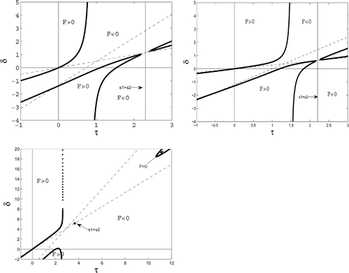
From the explicit form of the domain boundary, one sees that, in general terms, the stability domain widens if p ₁ or p ₂ is increased.

As an example, consider the situation where p ₁, q ₁, p ₂, q ₂>0 are fixed. Assume that also K, m, a, b are given. If B>B¯, then the coexistence point of Equation (2) is stable. Now assume that B<B¯. Then the coexistence point of Equation (2) is unstable. If, however,

then the coexistence point becomes stable for a sufficiently large exploitation rate c. Notice that the coordinates of the coexistence point do not depend on the parameter c but the formula for the determinant has c as a factor. Hence, for given τ, every point can be reached (draw a vertical line in Figure 2).

We also consider two limiting scenarios where the system with a quiescent phase has only dimension 3:

Scenario I: Only the prey takes refuge, p ₂=q ₂=0.

Then the stability domain is

with

It is evident that the stability domain widens with increasing p ₁ and shrinks with increasing q ₁.

Scenario II: Only the predator takes refuge, p ₁=q ₁=0.

Then the stability domain is

with

Now the situation is more complicated. Clearly the stability domain shrinks if q ₂ is increased. The dependence on p ₂ is more involved. If p ₂<q ₂, then the domain widens in all directions if p ₂ is increased. But if p ₂ is large, then near τ=0 the domain can shrink with increasing p ₂.

Hence we have the remarkable finding that in some parameter ranges increasing the length of the quiescent period or shortening of the active period of either the predator or the prey (the other species having no quiescent phase) widens the stability window.

Finally we show that the system has some standard properties of a useful biological model.

Theorem 2

Non-negative solutions of the system (3) exist for all positive times. The system in has a compact global attractor.

3. Proof of Theorem 1

We compute the Jacobian matrix of the system (3) at the coexistence point and then the characteristic polynomial (we suppress the details of the derivation)

The coefficients are (recall (7))

The stability problem can be discussed in terms of the Routh–Hurwitz criterion 3. The Hurwitz conditions (with a ₀=1) read

If these inequalities are satisfied, then also a ₄>0 (recall that a ₄ is the product of the four roots). Hence the Hurwitz conditions are equivalent to

Hence we have three linear inequalities for τ and δ,

We find

Now the last condition in Equation (18) assumes the form

We denote the left-hand side of Equation (21) by and collect terms in powers of δ:

The function F is a cubic in two variables τ, δ. The crucial Hurwitz condition is . The null set of the function F divides the τ, δ-plane into sectors in which F is either positive or negative. We write F in the form

We see that if one of the three functions φ _i vanishes, then F<0. Hence the union of the three straight lines lies in the domain where F is negative.

Qualitative properties of the set :

• (i) The function F is a cubic in τ and δ. The null set has several branches which may intersect, see Figure 2. F is cubic in τ and quadratic in δ. Hence for any given τ, the equation F=0 has at most two solutions δ. For any given δ, the equation F=0 has at most three solutions τ.

• (ii) Asymptotes. The graph of F=0 has a vertical asymptote at τ=p. The leading homogeneous part of degree 3 is a linear combination of , , and τ³ with non-trivial coefficients. We divide by τ³ and get a quadratic equation for the directions of the asymptotes

  Notice that the numerator in the coefficient of the linear term is positive. The discriminant of this equation is
  It follows that there are two real roots (or a double real root). These roots are both positive because of the signs of the coefficients in Equation (24). Hence we have two asymptotes with positive directions (which may degenerate if the discriminant vanishes).

• (iii) Zeros and poles. The δ²-term vanishes for . The function F(0, δ) has the root δ=0 and a second zero δ₋ which is negative. The function F(τ, 0) has the zero τ=0 and two positive roots

  We call the smaller of these roots z ₁ and the larger z ₂. Depending on the parameters, each of the expressions (25) may be the larger root.

• (iv) The function has a double zero at

  and no other zeros.

• (v) The function F(p, δ) has one zero (the other zero has moved to infinity), where

  We discuss the sign of ˆδ. There are three cases.

• Case 1a. p<z ₁<z ₂. Then p ₂<q ₁ and . Then N>0 and . Hence .

• Case 1b. z ₁<p<z ₂ with two subcases.

• Case 1ba. p ₂<q ₁ and . Then N<0 and, as in Case 1a, D<0. Hence .

• Case 1bb. p ₂>q ₁ and . Then N<0. Multiply the second inequality by p ₂−q ₁>0 and get

  and hence D<0 and .

• Case 2. z ₁<z ₂<p. Then p ₂>q ₁ and . Then N>0. But D and hence ˆδ may be positive or negative.

• (vi) Now we describe the null set for the same three cases (Figure 2).

Case 1a

p<z ₁<z ₂. For τ=0, there is a zero δ=0 and a negative zero δ₋. Hence the null set has two branches through (0, 0) and (0, δ₋). Along the branch through (0, 0) the variable δ goes to infinity as τ→p. The branch through (0, δ₋) passes through , then through (z ₁, 0), while a third branch starts with τ>p, and δ<0 and passes through the zero (z ₂, 0). Since the line lies in F<0, it follows that the second and the third branch intersect at a point on the line . The value of δ at this point is δ*.

Case 1b

z ₁<p<z ₂. The picture is similar to that of Case 1a. Along the branch through (0, 0) the variable δ goes to +∞ as τ→p. The second branch passes through (0, δ₋) and (z ₁, 0) and then through with , while the third branch is asymptotic to τ=p and passes through (z ₂, 0). The second and the third branch intersect at .

Case 2

z ₁<z ₂<p. Along the branch through (0, 0) the variable δ increases and the branch becomes asymptotic to τ=p. The branch through (0, δ₋), with δ₋<0, passes through (z ₁, 0) into δ>0, then bends down and passes through (z ₁, 0), and finally is asymptotic to τ=p with . Now there are two subcases.

Case 2a

. Then the branch through (0, δ₋) crosses the line τ=p at while the branch through (0, 0) stays in τ<p.

Case 2b

. Then the branch through (0, 0) crosses the line τ=p at with τ increasing to some maximal value and then bends back and becomes asymptotic to τ=p.

There is a third branch which forms a hairpin with two asymptotes in , and there is a fourth branch which contains the point with . In typical examples, this point is isolated. We cannot exclude that for certain choices of the parameters, this point is part of a closed curve or joins with the hairpin. Also in Cases 1a and 1b it could be that for certain parameter configurations the crossing of branches at breaks up into two hairpins.

We know that F>0 above the first branch and that the three straight lines φ _i =0 are in the domain where F<0. Hence in the domain above the first branch, we have F>0 and also φ _i >0 for i=1, 2, 3. So the domain above the first branch belongs to the stability domain.

There are two more domains where F>0. The domains are bounded by the second and the third branch. With respect to the three straight lines, they lie on the side where the inequalities (19) are not satisfied. Hence, Equation (8) is the stability domain.

Conclusion: In all cases, there is a part of the stability domain which lies in the positive quadrant of the τ, δ-plane. This domain is bounded by the positive δ-axis and the first branch of the null set of F. The boundary is asymptotic to the line . So, generally speaking, the stability window gets wider when p ₁+p ₂ is increased.

This observation makes sense in terms of the biological interpretation. Increasing p ₁ or p ₂ puts more prey or predators into the quiescent phase. However, the details of the parameter dependence are more complicated, as can be seen from the discussion of the two limiting cases.

Historical comment: The classification of cubic algebraic equations in two variables starts with the 72 cases of Newton and extends through the 19th century with the work of Plücker 17 (who distinguished 219 cases) and later of Brill and Noether 1. Although this problem lies at the basis of algebraic geometry, it seems that many elementary questions have not been pursued after these authors. Of course, our three cases appear among the cases of Plücker (Cases 1a and 1b correspond to his Cases I.4 or II.4, three branches of which two intersect, but only once, while Case 2 corresponds to I.2 or II.2, three branches without intersection and an isolated point). But we must be aware that the general cubic depends on 10 real parameters, whereas the 10 coefficients of our cubic depend only on four positive parameters. To investigate how this four-parameter family is embedded in the general case would go far beyond the scope of the present paper.

Next we look at the limiting scenarios.

Scenario I: The characteristic polynomial is

with

The Hurwitz conditions are

These conditions are equivalent to

Scenario II: Now the coefficients of the characteristic polynomial are

and the Hurwitz conditions are

These conditions are equivalent to

4. Proof of Theorem 2

Proof of global existence

The orthant R ₊ ⁴ is positively invariant. We consider non-negative solutions. Along any solution, we have

and

which shows that the solution grows at most exponentially and hence exists for all time.

Lemma 1

Suppose we are given two continuously differentiable functions x(t) and y(t) which are non-negative and satisfy the inequalities

with positive constants . Choose any and define . Then there is a t ₀≥0 (depending on μ and on the particular function (x, y)) such that y(t)≤ν and for t≥t ₀.

Proof

Define the function, for ,

This function is continuous and piecewise continuously differentiable. Its level sets for V≥0 are the trapezoidal polygons

The function V is not differentiable along the line x=μ, but this line is transversal to the boundary at x=μ, . Let for some κ>0.

• (i) If x¯<μ, then and near . Hence for (x, y) close to

• (ii) If x¯>μ, then near and

• (iii) If x¯=μ, then use the convexity of the level set to show that [xdot]+y˙ is pointing strictly inward.

Hence V is strictly decreasing as long as V>0. Now the lemma is proved.   ▪

Proof of Theorem 2

(i) From we have and thus, for x=u/K,

Hence

Apply Lemma 1 and get the following. Choose M>K and N=p ₁ M/q ₁. In the u, w-plane define a trapezoidal domain with four edges

and the cylinder set . Then every solution in ends up in .

• (ii) Define

Choose M>K. Then along any solution, we have, using (37),

with

Also, we have

with

Now apply Lemma 1 and get boundedness.   ▪

References

- Brill , A. and Noether , M. “ Die Entwicklung der Theorie der algebraischen Funktionen in aelterer und neuerer Zeit ” . 1892 – 93 . Reimer, Berlin : Jahresber. der Deutschen Mathematiker-Vereinigung III, 1894 .
- Cheng , K.-S. 1981 . Uniqueness of a limit cycle for a predator-prey system . SIAM J. Math. Anal. , 12 : 541 – 548 .
- Gantmacher , F. R. 1959 . The Theory of Matrices , Vol. 1, 2 , New York : Chelsea Publishing Co .
- Gyllenberg , M. and Webb , G. F. 1989 . Quiescence as an explanation of Gompertzian tumor growth . Growth Develop. and Aging , 53 : 25 – 33 .
- Hadeler , K. P. 2007 . Quiescent phases and stability . Lin. Alg. Appl. , 428 : 1620 – 1627 .
- Hadeler , K. P. and Lewis , M. A. 2002 . Spatial dynamics of the diffusive logistic equation with a sedentary compartment . Can. Appl. Math. Quart. , 10 : 473 – 499 .
- Hadeler , K. P. and Hillen , T. 2007 . “ Coupled dynamics and quiescent states ” . In Math Everywhere , 7 – 23 . Berlin : Springer .
- Hillen , T. 2003 . Transport equations with resting phases . Eur. J. Appl. Math. , 14 : 613 – 636 .
- Hillen , H. and Hadeler , K. P. 2005 . “ Hyperbolic systems and transport equations in Mathematical Biology ” . In Analysis and Numerics for Conservation Laws , Edited by: Warnecke , G. 257 – 279 . Springer .
- Holling , C. S. 1965 . The functional response of predators to prey density and its role in mimicry and population regulation . Mem. Ent. Soc. Can. , 45 : 65
- Jäger , W. , Krömker , S. and Tang , B. 1994 . Quiescence and transient growth dynamics in chemostat models . Math. Biosci. , 119 : 225 – 239 .
- Kolmogorov , A. N. 1936 . Sulla teoria di Volterra della lotta per la esistenza . Giorn. Ist. Ital. Attuar. , 7 : 74 – 80 .
- Lewis , M. A. and Schmitz , G. 1996 . Biological invasion of an organism with separate mobile and stationary states: modeling and analysis . Forma , 11 : 1 – 25 .
- Malik , T. and Smith , H. L. 2006 . A resource-based model of microbial quiescence . J. Math. Biol. , 53 : 231 – 252 .
- Neubert , M. G. , Klepac , P. and van den Driessche , P. 2002 . Stabilizing dispersal delays in predator-prey metapopulation models . Theor. Popul. Biol. , 61 : 339 – 347 .
- Pachepsky , E. , Lutscher , F. , Nisbet , R. M. and Lewis , M. A. 2005 . Persistence, spread and the drift paradox . Theor. Popul. Biol. , 67 : 61 – 73 .
- Plücker , J. 1835 . “ System der analytischen Geometrie, auf neue Betrachtungsweisen gegründet, und insbesondere eine ausführliche Theorie der Curven dritter Ordnung ” . Berlin : Duncker und Humblot .
- Rosenzweig , M. L. 1971 . Paradox of enrichment: destabilization of exploitation ecosystems in ecological time . Science , 171 : 385 – 387 .
- Rosenzweig , M. L. and MacArthur , R. H. 1963 . Graphical representation and stability conditions of predator-prey interactions . Amer. Nat. , 97 : 209 – 223 .
- Satnoianu , R. A. and van den Driessche , P. 2005 . Some remarks on matrix stability with applications to Turing instability . Lin. Alg. Appl. , 398 : 69 – 74 .