Flu epidemics: a two-strain flu model with a single vaccination

Abstract

Vaccination is considered one of the most effective control measures for influenza. However, when a virus mutates and multi-strains appear in a population, implementing a vaccine for one strain may affect the spread of the other strains. In this paper, we propose a two-strain model and investigate the effects of a single-strain vaccine on the dynamics of this two-strain model. The global dynamics of the model are completely determined through suitable Lyapunov functions. We show that if the basic reproduction number is less than one, then both strains die out; but when the number is larger than one, one or both of the strains become endemic depending on the parameter values. The theoretical results provide some useful information on the impact of the vaccination rate of this single-vaccine for one strain on the dynamics of the two strains.

Keywords:

• influenza
• epidemics
• vaccination
• equilibrium
• basic reproduction number
• global asymptotic stability
• Lyapunov function

AMS Subject Classification :

• 34K18
• 34K20
• 92D30

1. Introduction

Influenza, commonly known as flu, is one of the long-lasting major health issues throughout the world. This single disease alone causes hundreds of thousands of deaths annually. A pandemic flu is even more severe, in terms of spatial spread, infection and casualty, than a seasonal flu. During the last century, three major flu pandemics took place. Among them, the Spanish flu in 1918 is known as the most devastating pandemic. It is estimated 14 that the Spanish flu claimed around 40–50 million deaths (as much as 3% of the total population), and it also infected 20–40% of the whole population. Forty years later, in 1957–1958, human beings experienced another flu pandemic known as the Asian flu or bird flu, which caused more than two million deaths 14. Unlike the Spanish flu, this time the infection-causing virus was detected earlier due to the advancement of science and technology. A vaccine was made available but with limited supply. After a decade (in 1968), a flu pandemic that originated again from Hong Kong hit mankind. That flu pandemic also claimed one million lives 14. Beside these three major ones, there are some other flu pandemics spreading among nations on smaller scales. For instance, the 2009 H1N1 swine flu is one of the more publicized pandemics that attracted the attention of all scientists and health professionals in the world and made them very much concerned. The pandemic, however, did not result in great casualties like before. As of July 2010, only about 18,000 related deaths had been reported 15.

Due to the severeness of the flu endemic, extensive and intensive research has been done, focusing on understanding the transmission mechanism and control strategies (see, e.g. 2 12 and references therein). Among various control strategies, vaccination is considered to be the most effective one. A vaccine typically contains an agent that resembles a disease-causing microorganism which stimulates the body's immune system to recognize the agent as a foreigner. Thus, whenever such a microorganism is encountered within a host, the immune system will destroy it. This kind of phenomenon is known as immunity. The immunity can also be produced through infection. Once an individual has recovered from an infection, his/her immune system can recognize the microorganism that caused the infection as a harmful foreigner. The immune system may even identify a microorganism that is similar to one encountered before. This is known as ‘cross immunity’.

Unlike measles (which are generated by a single virus 3), flu viruses are able to mutate, which give them the opportunity to elude the immune system of an individual. There are three major types of flu viruses: type A, B and C. Each type has several sub-types and strains. A sub-type of a virus is the resultant of a drastic antigenic change known as ‘antigenic shift’ that occurs occasionally. However, there are small but continual changes taking place in a virus antigen known as ‘antigenic drift’ that produce a newer strain. Once a newer virus strain appears, the antibodies against the older strain no longer recognize the newer one, and infection with a new strain can occur. This is one of the main reasons why people can get flu infections more than once. A very good example is the 2009 H1N1 A virus. It was reported that ‘Antigenic characterization of 2009 influenza A (H1N1) viruses indicates that these viruses are only distantly related antigenically and genetically to seasonal influenza A (H1N1) viruses, suggesting that little to no protection would be expected from vaccination for the seasonal influenza vaccine’ (see, e.g. 5). Since making a vaccine for a newly merged strain takes quite long, a very natural yet practical question would be: in a situation where there are two strains of flu but only one vaccine for the older strain is available, how would the implementation of this vaccination affect the spread of the newer strain. As CBC News broadcast, ‘preliminary research suggests the seasonal flu shot may put people at greater risk for getting swine’ 4. In this research, we will investigate such an effect of the vaccination of the current strain towards the newer strain, by proposing and analysing a mathematical model for such a scenario. This problem is strongly motivated by the 2009 swine influenza pandemic, when the seasonal flu was also spreading in many places.

The rest of this paper is organized as below. In Section 2, following the line of 3, we formulate a two-strain influenza model in which a vaccination compartment with strain 1 is introduced for our purpose. In Section 3, we investigate the dynamics of this model system. By solving for all possible equilibria, computing the basic reproduction number, analysing the characteristic equation and employing Lyapunov functions, we are able to completely determine the global dynamics. In Section 4, we explore biological implications of some of the theoretical results obtained in Section 3; in particular, we discuss the impact of the vaccination with strain 1 on the spread of strain 2.

2. The model

The structure of the model we use in this paper follows that in Castillo-Chavez et al. 3. We are interested in the effect of a vaccination for one strain of influenza on the spread of another strain. We assume that a type of influenza virus, called strain 1, which is moderate in virulence, prevails in the population and a vaccine is available for the current strain. A new strain, called strain 2 which is antigenically far related to the existing subtype and which has severe virulence effect, suddenly appears in the same host population. Substantial time is required to produce a safe and effective vaccine for the newer strain, and there is no pre-existing immunity in the population. To model the disease dynamics in such a scenario, we follow the tradition of dividing the population N into five compartments: susceptible, immunized with the vaccination for strain 1, infected with strain 1, infected with strain 2, and finally, recovered. The subpopulations in these compartments are denoted by S, V ₁, I ₁, I ₂ and R, respectively.

For simplicity, we assume that there is a constant recruitment into susceptible class through birth and/or immigration, and we assume that there is no double infection. Susceptible individuals are vaccinated with constant rate r for strain 1, and are infected by strains 1 and 2 with transmission coefficients β₁ and β₂, respectively. The vaccinated individuals (V ₁) can also be infected by strain 2 at the rate of κ. Once recovered from either strain 1 or 2, an individual remains in recovery class for good. The variables and parameters are summarized in Table 1 and the transfer diagram is shown in Figure 1.

Figure 1. Transfer diagram of the model (2).

Table 1. Description of variables and parameters of model (2).

Parameter	Description
Λ	Recruitment of individuals
1/μ	Average time of life expectancy
r	Rate of vaccination with strain 1
k	Transmission coefficient of vaccinated individuals to strain 2
β1	Transmission coefficient of susceptible individuals to strain 1
β2	Transmission coefficient of susceptible individuals to strain 2
1/γ1	Average infection period of strain 1
1/γ2	Average infection period of strain 2
ν1	Infection-induced death rate of strain 1
ν2	Infection-induced death rate of strain 2

With the above assumptions, the disease dynamics is then described by the following system of ordinary differential equations:

with , where , and . In the next section, we will analyse model to obtain some information on the impact of vaccination for strain 1 on the global disease dynamics.

3. Disease dynamics described by the model

By the standard theory of ODE, it is easy to show that for a set of non-negative values , the system (1) has a unique solution in [0, t _m ) for some t _m >0, which also remains non-negative. Adding all equations in (1), the total population N satisfies

The comparison theorem then implies that . Hence N(t) is bounded on [0, t _m ), and so are all components and R(t). This in turn shows that the solution exists globally, i.e. for all t≥0.

Since the equation for ˙ R is actually decoupled from the rest in Equation (1), we only need to consider dynamics of the following four-dimensional sub-system:

Moreover, form the ˙ I ₁ and ˙ I ₂ Equations in (2), one can see that for i=1, 2, I _i0>0 (=0 resp.) indeed implies I _i (t)>0 (=0 resp.) for all t>0.

3.1. Equilibria

The system (2) has the disease-free equilibrium . There are two possible single-strain-infection equilibria and where

and

with ˆ I ₂ being determined by the quadratic equation

where

Obviously, E ₁ is biological meaningful if and only if

Now we seek the condition under which E ₂ is biologically meaningful. Firstly, we note that C≥0 is equivalent to

We claim that Equation (5) implies B>0. Otherwise, B≤0, which is equivalent to

Then, combining Equations (5) and (6) leads to

a contradiction. Thus, C≥0 implies B>0. By the property of quadratic equations, we know that when C>0, Equation (3) has no positive solution and hence, E ₂ is biologically meaningless. On the other hand, if C<0, then Equation (3) has a unique positive solution ˆ I ₂. Therefore, E ₂ is biologically meaningful if and only if C<0, that is,

It is also possible for the model (2) to have a double-strain-infection equilibrium (all components are positive) where

It is easily seen that I ₂*>0 if and only if

Also, in order for I ₁*>0, if and only if

3.2. Basic reproduction number

The basic reproduction number, denoted by , is a parameter that plays an important role in determining the disease persistence. It is defined as ‘the expected number of secondary cases produced, in a completely susceptible population, by a typical infected individual’ (see, e.g. 1 6 13), and can be calculated by using the idea of next generation matrix 13. Below, we follow the setting-up and notations in 13 to compute for our model (2).

Let

The matrix F is non-negative and is responsible for new infections, while the V is invertible and is referred to as the transmission matrix for the model (2). It follows that

The basic reproduction number is then given by the spectrum radius of FV ⁻¹, that is,

Define

By the meanings of the parameters involved, one easily sees the biological meanings of for i=1, 2: is the (average) number of secondary cases of strain i produced by an single infected individual with strain i during his/her infective period. The basic reproduction number can then be written as

By Theorem 2 in 13, we have the following theorem relating the stability/instability of E ₀ to the value of .

Theorem 3.1

The DFE E ₀ is asymptotically stable, if ; and it becomes unstable if .

In terms of the dynamical systems theory, the loss of stability of E ₀ should cause some new phenomenon. It turns out, as in other epidemic models, that the occurrence of new equilibrium is the new phenomenon. Indeed, this can be seen from the above theorem and the fact that when , then neither Equation (4) nor (7) holds; and when , then either Equation (4) or (7) holds, implying that either E ₁ or E ₂ comes into existence.

3.3. Global stability of equilibria

In the previous section, we have seen that when , the disease-free equilibrium E ₀ is asymptotically stable. We show that E ₀ is actually globally asymptotically stable in this case. After this, we will move on to explore the global stability of other possible equilibria, under appropriate conditions. To this end, we employ Lyapuov functions of very classic forms used recently by 7 8 10. Such Lyapunov functions all take advantage of the properties of the function

which is positive in ℛ₊ except at x=1, where it vanishes. The key for the success of such a Lyapunov function V lies in appropriately organizing terms in the derivative of V along the model system to achieve the optimal benefit. Fortunately, the recent work 7 has established some very useful (and precise in some sense) guidelines for this purpose, by using results from combinatory and graph theory. We will follow these guidelines to achieve our goal.

Theorem 3.2

The DFE E ₀ is globally asymptotically stable if\enspace .

Proof

Consider the Lyapunov function

Obviously, V is non-negative in the positive cone and attains zero at E ₀. We need to show ˙ V is negative definite. Differentiating V along the trajectories of Equation (2), we obtain

Using the model equations and rearranging the related terms, we get

If , then and . By these and the relation of geometric and arithmetic means, we conclude ˙ V≤0, with equality holding only at the equilibrium E ₀. Therefore, E ₀ is globally asymptotically stable if .   ▪

We have seen from above that when , then E ₀ becomes unstable and at least one of the E ₁ and E ₂ exists. We now investigate the global stability of these two possible single-strain equilibria.

Theorem 3.3

Assume that E ₁ exists (i.e. Equation (4) holds). If

then, E ₁ is globally asymptotically stable.

Proof

Consider the Lyapunov function

By the properties of g(x), we know that the function V is non-negative in the positive cone and attains zero at E ₁. We need to show ˙ V is negative definite. Differentiating V along the trajectories of Equation (2), we obtain

Using the equations in (2), taking advantage of the equilibrium equations for E ₁ and rearranging the terms, we get

Now Equation (10), together with the relation of geometric and arithmetic means, implies that ˙ V≤0 with the equality holding only at the equilibrium E ₁. By the Lyapunov–LaSalle theorem 9, we conclude that E ₁ is globally asymptotically stable in , completing the proof.   ▪

Remark 3.4

Note that Equation (4) is equivalent to , and the opposite of Equation (7) is

Thus, if E ₁ exists but E ₂ does not exist ,

implying that Equation (10) holds and hence, E ₂ is globally asymptotically stable.

Remark 3.5

If the inequality in Equation (10) is reversed, that is, if , then E ₁ becomes unstable. To see this, we compute the Jacobian matrix of model (2) at E ₁:

It is easy to see J(E ₁) has the principal eigenvalue

Thus, if\enspace , then ¯η>0 and hence, E ₁ is unstable, having a one-dimensional unstable manifold pointing to the interior of the .

Parallel to Theorem 3.3, we have the following theorem for E ₂.

Theorem 3.6

Assume that E ₂ exists (i.e. Equation (7) holds). If

then E ₂ is globally asymptotically stable.

Proof

The proof of this theorem is symmetric to that of Theorem 3.3, and hence we omit some details. Let us consider the Lyapunov function

Differentiating V along the trajectories of Equation (2), we obtain

Using the Equations in (2) and rearranging the terms, we get

By Equation (11) and the relation of geometric and arithmetic means, we conclude that ˙ V≤0, and the equality holds only at E ₂. By the Lyapunov–LaSalle theorem, we conclude that E ₂ is globally asymptotically stable in , completing the proof of the theorem.   ▪

Remark 3.7

The existence of E ₂ (i.e. I ₂>0, or Equation (7)) implies . On the other hand, the opposite of Equation (4) is Therefore, if E ₂ exists but E ₁ does not exist, then Equation (11) holds and hence, E ₂ is globally asymptotically stable.

Remark 3.8

If the inequality in Equation (11) is reversed, that is, if , then E ₂ becomes unstable. To show this, we first calculate the Jacobian matrix of Equation (2) at E ₂:

It is easy to see that J(E ₂) has the principle eigenvalue

Thus, if\enspace , then ˆη>0, and hence, E ₂ is unstable, having a one-dimensional unstable manifold pointing to the interior of .

Theorem 3.9

The endemic equilibrium E*, as long as it exists, is always globally asymptotically stable in the interior of .

Proof

Assume E* exists. Then the following function is well defined in :

Differenting V along the trajectories of Equation (2), we obtain

Again, by the relation of geometric and arithmetic means, we conclude that ˙ V≤0, and the equality holds only at E*. Therefore, E* is globally asymptotically stable and the proof is completed.   ▪

We have established the global stability of E* whenever it exists, and we have known that E* exists if and only if both Equations (8) and (9) hold. On the other hand, by Theorems 3.2–3.6 and Remarks 3.4–3.8, we know that E* can exist only when and . Obviously, the condition is exactly Equation (8). Tedious but straightforward verification shows that is equivalent to Equation (9). Combining this analysis with Theorem 3.9, we obtain the following.

Corollary 3.10

If

and

both hold, then there is a positive (double-strain-infection) equilibrium E* which is globally asymptotically stable in the interior of .

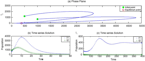
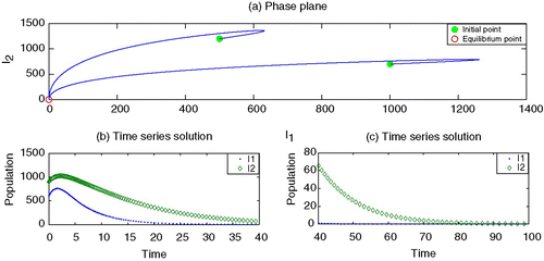
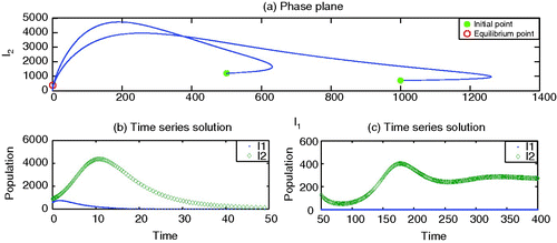
To conclude this section, we include some numeric simulations to demonstrate the results obtained above. Our intention is to observe the effect of vaccination for strain 1 on the infection with strain 2 when the transmission coefficients, β₂ from S to I ₂, and κ from V ₁ to I ₂ are different.

To begin, we set the parameter values, without vaccination, which generate Figure 2 depicting strain 1 as endemic but strain 2 as dying out. By adding the vaccination for strain 1 with an appropriate rate r>0, it is observed in Figure 3 that strain 1 may also die out. Here we choose values of κ smaller than β₂. However, the increased values of κ may facilitate strain 2 to survive and becomes endemic, as shown in Figure 4.

Figure 2. Endemic with strain 1. Parameter values are β₁=0.00003, β₂=0.00002, γ₁=0.07, γ₂=0.09, ν₁=0.10, ν₂=0.10, r=0.0, κ=0.00001, μ=0.02 and Λ=200.

Figure 3. Stable disease-free equilibrium: both strain die out. Parameter values are β₁=0.00003, β₂=0.00002, γ₁=0.07, γ₂=0.09, ν₁=0.10, ν₂=0.10, r=0.60, κ=0.00001, μ=0.02 and Λ=200.

Figure 4. Endemic with strain 2 by increasing κ. Parameter values are β₁=0.00003, β₂=0.00002, γ₁=0.07, γ₂=0.09, ν₁=0.10, ν₂=0.10, r=0.60, κ=0.00003; μ=0.02 and Λ=200.

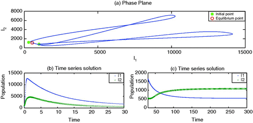
The model also demonstrates possible co-infections as shown in Figure 5, with the parameter values given in the caption of this figure.

Figure 5. Endemic with both strains. Parameter values are β₁=0.0005, β₂=0.0002, γ₁=0.08, γ₂=0.09, ν₁=0.01, ν₂=0.01, r=0.40, κ=0.0003, μ=0.02 and Λ=200.

4. Discussion

In this paper, we propose a system of ordinary differential equations to model the disease dynamics of two strains of influenza with only a vaccination for strain 1 being implemented. Investigated are the topics of existence and non-existence of various equilibria and their stabilities. Unlike most other works on epidemic models where only local stability are addressed, here we are able to obtain global stability for each of these equilibria under respective and sharp (necessary and sufficient) conditions.

For convenience of discussing the implications of these mathematical results, let us rewrite the two key in-direct parameters and in terms of the direct model parameters as shown below:

Since our major concern is the impact of the vaccination on disease dynamics, let us consider these two parameters as functions of the vaccination rate r. One can easily see that is decreasing in r with

and is increasing in r if ; decreasing in r if ; and remains unchanged in r if . It is also obvious that

With the above information and the results in Section 3, we conclude that while the vaccination is always beneficial for controlling strain 1 (as expected), its impact on strain 2 depends on the values of β₂ and κ: if , it plays a positive role; and if , it has a negative impact in controlling strain 2. This is natural and reasonable because larger κ (than β₂) means that vaccinated individuals are more likely to be infected by strain 2 than those who are not vaccinated, and thus, is helpful to strain 2. Smaller κ (than β₂) implies the opposite. For example, if and values of the model parameters are such that

then, sufficiently large r indeed can help reduce to some value less than 1, helping in eliminating strain 2. In opposite, if and the values of the model parameters are such that

strain 2, which is otherwise becoming extinct, may become endemic when vaccination rate is sufficiently large.

From the above discussion, we see that introduction of a vaccination for strain 1 does have an influence on strain 2 and it can even result in the persistence of strain 2. Such a feature has also been numerically observed in 11 where the authors used a similar two-strain model containing a vaccination for newborns and found that (numerically) there is a vaccine level above which the second strain can emerge as a result of vaccination campaign. Unlike 11, our model does not incorporate super-infection but also exhibits co-circulation of strains under some conditions.

The model can be further modified to contain two vaccinations (the situation in late 2009 when the vaccine for the swine flu also became available), as well as partial cross-immunity and super-infection. It is also worthwhile to consider the effect of delay on vaccine-induced immunity. We leave these as possible future projects.

Acknowledgements

We thank the referee for his/her valuable comments which have led to an improvement in the presentation of the paper. This study was partially supported by NSERC and MITACS of Canada, and by a Premier's Research Excellence Award of Ontario.

References

- Anderson , R. M. and May , R. M. 1991 . Infectious Diseases of Humans , Oxford : Oxford University .
- Andreasen , V. , Lin , J. and Levin , S. A. 1997 . The dynamics of cocirculating influenza strains conferring partial cross-immunity . J. Math. Biol. , 35 : 825 – 842 .
- Castillo-Chavez , C. , Hethcote , H. W. , Andreasen , V. , Levin , S. A. and Liu , W. M. 1989 . Epidemiological models with age structure, proportionate mixing, and cross-immunity . J. Math. Biol. , 27 : 233 – 258 .
- CBC, Seasonal flu shot may increase H1N1 risk. Available at http://www.cbc.ca/health/story/2009/09/23/flu-shots-h1n1-seasonal.html
- Centre for Disease Control and Prevention (2010). Available at http://www.cdc.gov/flu/weekly/09-2010
- Diekmann , O. , Heesterbeek , J. S.P. and Metz , J. A.J. 1990 . On the definition and the computation of the basic reproduction ratio R0 in models for infectious diseases in heterogeneous populations . J. Math. Biol. , 28 : 365
- Guo , H. , Li , M. Y. and Shuai , Z. 2008 . A graph-theoretic approach to the method of global Lyapunov functions . Proc. Am. Math. Soc. , 136 ( 8 ) : 2793 – 2802 .
- Korobeinikov , A. and Maini , P. K. 2004 . A Lyapunov function and global properties for SIR and SEIR epidemiological models with nonlinear incidence . Math. Biosci. Eng. , 1 : 57 – 60 .
- LaSalle , J. P. 1976 . The Stability of Dynamical Systems , Philadephia : SIAM .
- McCluskey , C. C. 2010 . Global stability for an SIR epidemic model with delay and nonlinear incidence . Nonlinear Anal. RWA , 11 : 3106 – 3109 .
- Mclean , A. R. 1995 . Vaccination, evolution and changes in the efficacy of vaccines: A theoretical framework . Proc. R. Soc. Lond. B , 261 : 389 – 393 .
- Nishiro , H. and Iwata , K. 2009 . A simple mathematical approach to deciding the dosage of vaccine against pandemic H1N1 influenza . Euro Surveill. , 14 : 57 – 60 .
- van den Driessche , P. and Watmough , J. 2002 . Reproduction numbers and subthreshold endemic equilibria for compartmental models of disease transmission . Math. Biosci. , 180 : 29 – 48 .
- World Health Organization (2010). Available at http://www.wpro.who.int/vietnam/sites/dcc/pandemic_-flu/10things_-about_-pandemic_-flu.htm
- World Health Organization (2010). Available at http://www.who.int/csr/don/2010_-04_-09/en/index.html