Global stability in a multi-species periodic Leslie–Gower model

Abstract

We consider a population model consisting of d species interacting in a p-periodic environment and modelled by a d-dimensional system of Leslie–Gower-type difference equations (coupled Beverton–Holt equations). It is shown that if the interspecific competition (coupling) is sufficiently small and the inherent growth rate of each species is such that in the absence of competition each species will grow to its (positive) individual carrying capacity, then there is a positive asymptotically stable p-periodic state that globally attracts all positive initial states. Three examples are studied numerically in which the competition is large and the principle of competitive exclusion is observed. The rate of decay to extinction is observed to be sensitive to the inherent growth rate of the dying species. The individual carrying capacities are seen to play a determining role in the case of equal and large competition and equal inherent growth rates.

Keywords:

• periodic difference equation
• global stability
• Leslie–Gower model

AMS Subject Classification :

• 39A11
• 92
• 92D
• 92D25

1. Introduction

The study of competition models inevitably leads one to consider either the Lotka–Volterra model in the continuous case or the Leslie–Gower model 10 in the discrete case. The typical Leslie–Gower model consists of two Beverton–Holt equations with added coupling (interspecific competition). When the interspecific competition is strong, one species will be driven to extinction; the principle of competitive exclusion that is one of the important tenets in ecology (see 2 3 7 for results and many references to this phenomenon). In 11, global stability in a two-species model is considered using techniques of monotone systems 9. In 4, multi-species models are considered, taking into account harvesting and stocking.

See 6 for further results on stage-structured models for larvae, pupae and adults, the well-known ‘LPA’ model that is essentially a delay equation for the larvae and adults. In 5, non-equilibrium competitive coexistence for a two-species LPA model was explored and a boundary 2-cycle was established. See also 1 in which a two-species juvenile–adult model is studied with the assumption that there is no competition between juveniles and adults.

For the Beverton–Holt (scalar) equation, the issue of global asymptotic stability, even in the periodic case, has been settled in 8. Since the functions defining these equations, being fractional linear, form a semi-group ℬ under composition, the existence and global asymptotic stability of a periodic equation reduces to establishing a fixed point with the same property for a single (autonomous) equation. In fact, in 8, it was shown that ℬ is a sub-semi-group of the larger semi-group 𝒦 of continuous functions that are concave, increasing and cross the diagonal in . In 12, the result was extended to C ³ functions that are either concave increasing or convex decreasing and have non-negative Schwarzian. These conditions are satisfied by certain rational functions with the roots of the numerator interlaced with the roots of the denominator.

In this paper, we consider d species interacting in a periodic environment modeled by a d-dimensional system of Leslie–Gower-type equations, or equivalently coupled Beverton–Holt equations. It is assumed that the inherent growth rate of each species is such that in the absence of competition each species will grow to its (positive) individual carrying capacity. It is shown that if the interspecific competition (coupling) is sufficiently small, then there is a positive asymptotically stable periodic state that globally attracts all positive initial states.

We then study numerically, in three four-dimensional examples, some cases in which the interspecific competition is large. In the first example, we see that large competition against just species number one, not surprisingly, drives that species to extinction. In the second example, we see that an increase in the inherent growth rate for species one by a factor of 1.77 must be countered by a 4.3-fold increase in the competition by all three competing species in order to achieve the same rate of decay to extinction. In the third example, we make all the competition large and equal and all the inherent growth rates equal and observe that the species with the smallest individual carrying capacity is driven to extinction.

2. Autonomous two-dimensional case

We begin with a discussion of this case in order to develop some notation that will make the d-dimensional case easier to formulate and discuss.

The two-species Leslie–Gower model is usually written in the following form:

We propose the following equivalent form of Equation (1) that is a pair of coupled Beverton–Holt equations. In addition, we view a difference equation as a mapping and thus focus our attention on the right-hand side f:

Here the coupling parameters c _ij are the coefficients of interspecific competition. If both c _ij =0 and μ _i >1, the system is decoupled and each x _i (n) with x _i (0)>0 asymptotically approaches its carrying capacity (fixed point), K _i as n→∞.

Our next goal will be to develop a notation and some operations that will make it straightforward to consider higher-dimensional maps. For those familiar with Matlab programming, these operations will not seem so strange.

Let a be a scalar and u and v be column vectors in ℝ ^d and C an d×d matrix. Define, in addition to the usual inner product and linearity rules,

We may now now rewrite Equation (2) as

where the product in the denominator is the usual matrix–vector multiplication and ‘ ′’ means transpose.

To further simplify this and eliminate cumbersome notation, we define the parameters

With these, Equation (2) takes the form

This form is not specific to ℝ², but can be interpreted in ℝ ^d as well. With C ⁰=0, Equation (7) represents d independent Beverton–Holt equations.

3. Interior fixed point, autonomous case: p=1

We consider the positive cone

The condition for a fixed point of Equation (7) in 𝒞⁰ is just f(x)=x, which yields

or in two dimensions is just

Equation (9) is a simple linear system and we have the following theorem.

Theorem 3.1

Assume μ _i >1 for all i=1, 2, …, d and the coupling terms C ⁰ are sufficiently small. Then there exists a unique fixed point that reduces to when C ⁰=0.

The theorem applies equally well to any of the invariant coordinate ‘faces’

In order to study stability, we note the following lemma.

Lemma 3.2

The function f is bounded in . More precisely, each component function

Therefore,

We next define K _min and K _max to be the minimum and maximum of the K _i and b=K _min/2. We then have the following lemma.

Lemma 3.3

Assume each row c _i of the matrix C ⁰ in Equation (7) satisfies

where is the euclidean norm. Then the compact set

is invariant under the action of f, i.e.

The proof will follow by setting v=x in the next more general lemma needed later.

Lemma 3.4

Define as follows. Let be arbitrary and define (cf. Equation (7))

Assume the rows c _i of the matrix C ⁰ satisfy Equation (13). Then

Proof

Let denote the inner product of vectors p and q. For , the ith component of [fcirc] satisfies

This together with Equation (12) completes the proof.   ▪

3.1. Dynamic reduction

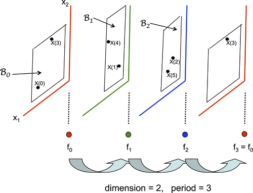
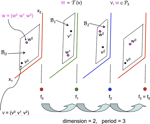
In the technique of dynamic reduction introduced in 14, one defines a class of p-periodic sequences of column vectors v _n :

For p=1, the case we are currently considering, the ‘sequences’ are independent of n, i.e. constant sequences. For each , one then looks at the ‘reduced’ version of difference equation with the right-hand side (7):

which is just a system of d uncoupled difference equations. Next define . We then have

Theorem 3.5

In addition to assume that the rows of C ⁰ satisfy

Then Equation (18) has a fixed point , thus establishing a mapping

For C ⁰ sufficiently small, 𝒯 is a contraction yielding a unique fixed point v*. In addition, v* is an exponentially asymptotically stable fixed point of Equation (7) that is globally attracting with respect to the cone 𝒞⁰ (Equation (8)).

Proof

Each component function [fcirc] _i in Equation (18) is fractional linear, concave increasing and from Equation (19) has a slope at the origin that is greater than one. Thus, either by 8 or 12, one obtains an exponentially asymptotically stable solution (fixed point) w _i and from Lemma 3.4, . This establishes Equation (20). Note that since w satisfies Equation (18),

and thus

from which it follows that 𝒯 is a contraction for C ⁰ sufficiently small. For the remaining details of the proof, see 14.   ▪

4. Periodic case: p>1

The periodic version of Equation (7) is , where

For the sake of simplicity of presentation, we shall work with the case where the dimension d=2, the period p=3 and only the individual carrying capacities K _i are periodic:

and

The evolution of the maps f _n along with the state variable x(n) is illustrated in the skew-product 13 setting (Figure 1).

Figure 1. Orbit in skew-product flow.

Before proceeding, however, let us prove the periodic version of Lemmas 3.2 and 3.4 in the general case.

Lemma 4.1

The functions f _n are bounded in . More precisely, each component function satisfies

Therefore,

Lemma 4.2

For define with

and set

and b=K _min/2. Assume each row c _{i, n} of the matrices in Equation (25) satisfies

where is the euclidean norm. Then the compact set

where

is invariant in the skew-product dynamical system, i.e.

Note: The set on the right is labelled with ‘j+1’ since it lies in the domain of f _j+1 with subscripts taken mod p (Figure 1).

Proof

Let denote the inner product of vectors p and q. For , the ith component of [fcirc] satisfies

This together with Equation (24) completes the proof.   ▪

4.1. Dynamic reduction: periodic case

To apply dynamic reduction, we first separate out the coupling terms in Equation (21) to obtain

or simply

We next define the class of three periodic sequences

where all subscripts are taken mod 3. For , we get the reduced equation

and

where again, for the sake of clarity, we have suppressed the periodic dependence in the μ _i and c _ij .

The difference equations on the right-hand sides of Equation (29) are uncoupled and each such equation is a three periodic concave increasing function mapping . By 8 12, we obtain an exponentially asymptotically stable periodic solution,

that globally attracts all initial states in the positive cone 𝒞⁰. Thus, we have the mapping (Figure 2).

Figure 2. Mapping 𝒯.

We next introduce the following notation: For and a periodic vector valued sequence of functions with we define . For a fixed with , and with define . For F=F(x, g), we will use ∂₁ F and ∂₂ F to mean differentiation with respect to the first and second arguments.

Referring to Equation (28), let us temporarily suppress the dependency of the F _j on g and define

so that the periodic solution (30) satisfies where n is understood ‘mod 3’. Then we see that the first element w ⁰ of the periodic solution (30) is a fixed point of the composite map,

In computing the derivative with respect to v, we need the following estimates:

where

and

Thus, from Equation (31), and recalling that we are taking the period p=3 for simplicity of presentation,

where

From the exponential asymptotic stability of w ⁰(v) as a periodic solution of the difference equation (28), one has

Thus has a bounded inverse and from Equation (32),

Next we define a norm in 𝒫₃ to be

Then it follows from Equation (33) that for δ∈(0, 1) and sufficiently small,

and from the mean-value estimate,

for any pair and t∈[0, 1]. Therefore,

and 𝒯 is a contraction. Thus, 𝒯 has a unique fixed point in . Being fixed under the action of 𝒯 means that when v* is inserted into Equation (28) in place of v, this equation has v* as its asymptotically stable three periodic solution, i.e. v* is the asymptotically stable three periodic solution of Equation (27).

The global asymptotic stability follows by the argument given in 14. Thus, we have established the following theorem.

Theorem 4.3

Consider the p -periodic, d -dimensional system (21) which we repeat: where

and assume and all the ‘ n ’ subscripts are understood ‘mod p ’. Then if the coupling is sufficiently weak, Equation (34) has a strictly positive, asymptotically stable p -periodic solution

Further, v* is globally attracting with respect to initial conditions x(0)>0.

5. Large inter-specific competition: numerical examples

In the previous sections, we considered the result of small inter-specific competition, i.e. small coupling C ⁰ in Equation (7) or Equation (34) in the periodic case. No species was driven to extinction and a coexistence state was established that attracted all initial states starting in the positive cone 𝒞⁰ defined in Equation (8).

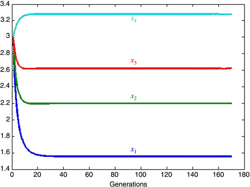
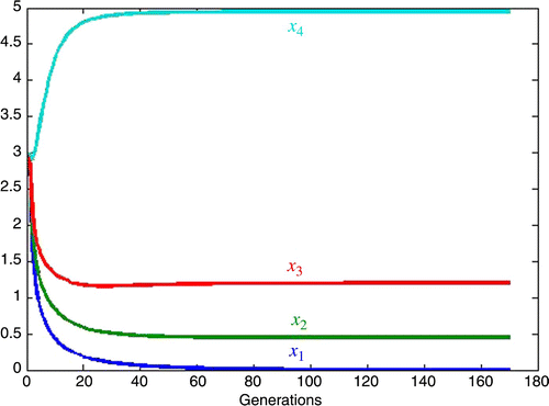
We now consider, in dimension 4, the effect of strong competition against species number one, x ₁, with inherent growth rates approximately equal in Section 5.1. Then, in Section 5.2, we increase the inherent growth rate for x ₁ and note the rather large increase in competition against x ₁ needed to achieve the same decay rate to extinction as in case 1. In Section 5.3, we consider the case of equal competition and equal inherent growth rates and see that the individual carrying capacities determine the species that goes extinct.

As a point of reference, let us consider an example of small competition with

Numerically, we find the attractive fixed point to be (Figure 3),

Figure 3. Coexistence.

5.1. Inherent growth rates approximately equal

We now consider the example in Equations (35) and (36) in which the inherent growth rates of all species are approximately equal and increase the competition against species one to . The attractive fixed point is now (Figure 4),

Figure 4. Large competition against species 1.

Specifically,

By increasing the competition against species 1 just 1.1% to the attractive fixed point remains unchanged to the accuracy shown, but species x ₁ approaches extinction much faster, viz.

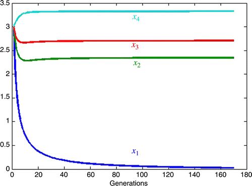
5.2. One dominant inherent growth rate

We now consider the example in Equations (35) and (36) except that now we take the inherent growth rate of species 1 to be 1.77 times that given in Equation (36). Thus, let

the attractive fixed point then becomes

For the attractive fixed point is

Thus, by increasing the inherent growth rate of species one from 1.3 to 2.3, a factor of 1.77, the competition against species one must be increased by a factor of 4.3 for all three competing species in order to achieve the same asymptotic rate to extinction.

By increasing the competition against species one by approximately 5.3% to the attractive fixed point remains unchanged to the accuracy shown, but species x ₁ approaches extinction much faster, viz.

Thus, increasing the competition by a factor only 5.3%, we see a much larger decay to extinction by species one.

5.3. Equal but large competition

Here we consider the case in which all the competition is equal and the inherent growth rates are equal. As a point of reference, consider the small competition case where in Equation (3),

The attractive fixed point is

Replacing C ⁰ by C=20C ⁰, it is no surprise that the individual carrying capacities K, the only parameters left that are not at parity with one another, determine the ordering of the coordinates of the fixed point

see Figure 5.

Figure 5. Extinction determined by carrying capacities.

6. Conclusions

We have studied d species interacting in a p-periodic environment and modeled by a d-dimensional system of Leslie–Gower-type equations (coupled Beverton–Holt equations). It is shown that if the interspecific competition (coupling) is sufficiently small and the inherent growth rate of each species is such that in the absence of competition each species will grow to its (positive) individual carrying capacity, then there is a positive asymptotically stable p-periodic state that globally attracts all positive initial states, i.e. coexistence.

We also study three cases of large competition, all of which lead to competitive exclusion with species one, x ₁ going extinct. In the first, we let the competition be unbalanced and discriminating against x ₁ with inherent growth rates approximately equal. In case 2, we increase the inherent growth rate for x ₁ by a factor of 1.77 and see that the competition against x ₁ must be increased by a factor of 4.3 in order to obtain the same rate of decay to extinction as in case 1. In case 3, we set all the competition equal and large and all the inherent growth rates equal and see that the ordering of the size of the species at equilibrium is the same as that of the individual carrying capacities, with the species having the least carrying capacity, x ₁, going extinct.

Acknowledgements

Robert J. Sacker is supported by the University of Southern California, Letters Arts and Sciences Faculty Development Grant. The author thanks the referee for their helpful suggestions.

References

- Ackleh , A. S. and Chiquet , R. A. Competitive exclusion in a discrete juvenile–adult model with continuous and seasonal reproduction . preprint (2010), to appear in J. Difference Equ. Appl. doi:10.1080/10236190903460420
- Ackleh , A. S. , Dib , Y. M. and Jang , S. R.J. 2005 . “ A discrete-time Beverton-Holt competition model ” . In Difference Equations and Discrete Dynamical Systems , Edited by: Allen , L. J.S. , Aulbach , B. , Elaydi , S. and Sacker , R. 1 – 9 . London : World Scientific .
- Ackleh , A. S. , Dib , Y. M. and Jang , S. R.J. 2007 . Competitive exclusion and coexistence in a nonlinear refuge-mediated selection model . Discrete Contin. Dyn. Syst. Ser. B , 7 ( 4 ) : 683 – 698 .
- AlSharawi , Z. and Rhouma , M. 2009 . Coexistence and extinction in a competitive exclusion Leslie/Gower model with harvesting and stocking . J. Difference Equ. Appl. , 15 ( 11 ) : 1031 – 1053 .
- Cushing , J. M. , Henson , S. M. and Roeger , L.-I. 2007 . Coexistence of competing juvenile–adult structured populations . J. Biol. Dyn. , 1 ( 2 ) : 201 – 231 .
- Cushing , J. M. and LeVarge , S. 2005 . “ Some discrete competition models and the principle of competitive exclusion ” . In Difference Equations and Discrete Dynamical Systems , Edited by: Allen , L. J.S. , Aulbach , B. , Elaydi , S. and Sacker , R. 283 – 301 . London : World Scientific .
- Cushing , J. M. , Levarge , S. , Chitnis , N. and Henson , S. M. 2004 . Some discrete competition models and the competitive exclusion pronciple . J. Difference Equ. Appl. , 10 ( 13–15 ) : 1139 – 1151 .
- Elaydi , S. and Sacker , R. J. 2005 . Global stability of periodic orbits of nonautonomous difference equations . J. Differential Equations , 208 ( 11 ) : 258 – 273 .
- Hirsch , M. W. and Smith , H. 2005 . Monotone maps: A review . J. Difference Equ. Appl. , 11 ( 4–5 ) : 379 – 398 .
- Leslie , P. H. and Gower , J. C. 1958 . The properties of a stochastic model for two competing species . Biometrika , 45 : 316 – 330 .
- Liu , P. and Elaydi , S. N. 2001 . Discrete competitive and cooperative models of Lotka-Volterra type . J. Comput. Anal. Appl. , 3 ( 1 ) : 53 – 73 .
- Sacker , R. J. 2010 . Semigroups of maps and periodic difference equations . J. Difference Equ. Appl. , 16 ( 1 ) : 1 – 13 .
- Sacker , R. J. and Sell , G. R. 1977 . Lifting properties in skew-product flows with applications to differential equations . Mem. Amer. Math. Soc. , 11 ( 190 )
- Sacker , R. J. and von Bremen , H. F. 2007 . Dynamic reduction with applications to mathematical biology and other areas . J. Biol. Dyn. , 1 ( 4 ) : 437 – 453 .