Passing to the limit 2D–1D in a model for metastatic growth

Abstract

We prove the convergence of a family of solutions to a two-dimensional transport equation with a non-local boundary condition modelling the evolution of a population of metastases. We show that when the data of the repartition along the boundary tend to a Dirac mass, then the solution of the associated problem converges and we derive a simple expression for the limit in terms of the solution of a 1D equation. This result permits us to improve the computational time needed to simulate the model.

Keywords:

• structured population dynamics
• cancer modelling
• angiogenesis

AMS Subject Classification :

• 35B30
• 92C50

1. Introduction

In the dynamical evolution of a cancer disease, some cancerous cells can detach from the primary tumour and spread in the organism to form secondary tumours, called metastases. These metastatic tumours can remain very small and beyond the detectable threshold with medical imaging techniques, for instance in the case of breast cancer, yet existence of occult micro-metastases at diagnosis is established 12.

A fundamental process in the tumoral growth, called neo-angiogenesis, consists in establishing a vascular network, which ensures to the tumour, supply of nutrients and the possibility to spread metastases in the organism. Thus, a therapeutic approach first proposed by Folkman 10 intends to block this process, aiming at starving the tumour by depriving it from nutrient supply. Though, the clinical question of optimal schedules for anti-angiogenic drugs is still open and is of fundamental importance 9 15 17.

In this perspective, the use of a mathematical model can lead to an interesting tool for the study in silico of the temporal administration protocols. Various models have been introduced for the evolution of the primary tumour, that can be separated between two classes: mechanistic models like 5 13 try to integrate the whole biology of the involved processes and comprise a large number of parameters; on the other hand, phenomenological models aim to describe the tumoral growth without taking into account all the complexity levels (see 18 for a review and 2 8 11 for examples). In 2000, Iwata et al. 14 proposed a phenomenological model for the evolution of the population of metastases, which was then further studied in 1 6. This model did not include the angiogenic process in the tumoral growth, hence we combined it with the tumoral model introduced by Hahnfeldt et al. 11, which takes into account angiogenesis. The resulting partial differential equation is part of the so-called structured population dynamics (see 16 for an introduction to the theory), it is a transport equation with a non-local boundary condition. The population of metastases is represented by a density ρ(t, X) with X being the structuring variable, here two-dimensional with x the size (=number of cells) and θ the so-called ‘angiogenic capacity’. The behaviour of each individual of the population, that is the growth rate G(X) of each metastasis is taken from 11 and is designed to take into account for the angiogenic process (see below for its expression). The equation writes

where Ω, the birth rate β(X), the repartition along the boundary N(σ) and the source term f(t) will be specified in the sequel (end of the Section 2.2), T is a positive time and ν is the unit external normal vector to the boundary . The theoretical study of this equation (existence, uniqueness, regularity and asymptotic behaviour) has been performed in 4. In the case of a non-autonomous growth velocity field G(t, X) which integrates the effect of the combination of an anti-angiogenic and a cytotoxic treatment, theoretical and numerical study of the model can be found in 3.

We formulate the biological assumption that the metastases are all born with size 1 and an angiogenic capacity close to a given value θ₀. This is translated in the model by considering a density N (repartition along the boundary) very concentrated around the value (1, θ₀), for instance with ϵ being a small parameter. In this paper, we demonstrate that the family of solutions to the problem (1) with data converges when ϵ goes to zero, to the measure solution of Equation (1) with the measure boundary data . Moreover, we derive a simple expression for involving the solution of a one-dimensional renewal equation. This permits us to simulate only the 1D equation rather than the 2D one in the applications and greatly improves the computational times.

2. Model

In this section, we describe the modelling approach used to take into account angiogenesis in the growth of each tumour taken from 11 and its combination with the metastatic model of 1 6 14. The mathematical analysis of the resulting model can be found in 4.

2.1. The model of tumoral growth under angiogenic control

Let x(t) denote the size (number of cells) of a given tumour at time t 11. The growth of the tumour is modelled by a Gompertzian growth rate and the equation is

where a is a parameter representing the velocity of the growth and θ the carrying capacity of the environment. The idea is now to take θ as a variable of the time, representing the degree of vascularization of the tumour and called ‘angiogenic capacity’. The variation rate for θ derived in 11 is

where the terms cx and represent, respectively, the endogenous stimulation and inhibition of the vasculature. The factor 2/3 comes from the analysis of 11 which concluded that the ratio of the stimulation rate over the inhibition one should be homogeneous to the tumoral radius to the square.

2.2. Renewal equation for the density of metastasis

We denote and . We define and where b is the maximal reachable size and angiogenic capacity for solving the system (2)–(3) (see 7 for a qualitative study of this ODE system). We consider each tumour to be a particle evolving in Ω with the velocity G. Writing a balance law for the density ρ(t, X), we have

that we endow with a null initial condition (no metastases at the initial time).

Metastasis do not only grow in size and angiogenic capacity, they are also able to emit new metastasis. We denote by the birth rate of new metastases with size and angiogenic capacity by metastases of size x and angiogenic capacity θ, and by the term corresponding to metastases produced by the primary tumour. Expressing the equality between the number of metastases arriving in Ω per unit time (l.h.s in the following equality) and the total rate of new metastases created by both the primary tumour and metastases themselves (r.h.s.), we should have for all t>0

We assume that the emission rate of the primary and secondary tumours are equal and thus take where X _p (t) represents the primary tumour and solves the ODE system (2)–(3) endowed with suitable initial conditions. We also assume that the newly created metastases have size x=1, in view of the following remarks (a) the passing vascular holes by which a metastasis pass to escape from the tumor have a diameter of order 100 nanometers. It is hard to imagine that more than one cell (whose typical size is the micrometer) could pass through such a small hole. (b) If the cells detach from the tumour, it means that the cadherin (transmembrane proteins responsible for cell–cell adhesion) rate falls. Thus, it seems unlikely that the cells lose cadherins from one side and keep sufficient to form a cluster on the other side. (c) Even in the assumption of the detachment of a cluster of cells, it would be composed of at most a dozen of cells since (a) and the hypothesis of size 1 cell for the neo-metastasis would stay in a convenient approximation. We also assume that there is no metastasis of maximal size b nor maximal or minimal angiogenic capacity because they should come from metastasis outside of Ω since G points inward all along . We assume that the vasculature of a neo-metastasis is independent from the one which emitted it, since each cell which detach then settles in a new environment which has no link with the one of the metastasis it comes from. Though, there is no experimental data to support this hypothesis up to our knowledge. Mathematically, this means that with N(σ) having its support in and describing the angiogenic distribution of the metastases at birth. We assume that all the metastases are born with an angiogenic capacity centred to a given value θ₀ with a variability parameter ϵ, as an approximation of the biological reality though we have no reference to provide about the shape of the angiogenic birth distribution of the metastases. We thus take N uniformly centred around a mean value θ₀

with ϵ a parameter of dispersion of the new metastases around θ₀. Following the modelling of 14 for the colonization rate β we take

with m the colonization coefficient and α the so-called fractal dimension of blood vessels infiltrating the tumour. The parameter α expresses the geometrical distribution of the vessels in the tumour. For example, if the vasculature is superficial, then α is assigned to 2/3 thus making x ^α proportional to the area of the surface of the tumour (assumed to be spheroidal). Otherwise, if the tumour is homogeneously vascularized, then α is supposed to be equal to 1. Assuming the equality of the integrands in Equation (5) in order to have the equality of the integrals, we obtain the boundary condition of Equation (1) where we denoted

3. Limit 2D–1D

A modelling hypothesis consists in considering that the newly created metastases are all born with the same given vasculature θ₀ and not distributed around this value. At least, the distribution N(σ) should be very concentrated around the value , that is . This is a simplification hypothesis which reduces the complexity of the model and thus its computational cost (see Section 4 for numerical illustrations), but we hope that it does not impoverish the model too much and that this one will still be able to describe the metastatic process. In this case, we would like to know if we can replace the function N by a Dirac mass centred in σ₀, in Equation (1). Mathematically, the problem is to determine whether the family of solutions to the problems

with converges when ϵ goes to zero and to determine its limit. See Figure 1 for an illustration. The theorem of this section demonstrates that the family converges to the measure solution (see below for the definition of ) of the problem

Figure 1. Phase plan of the systems (2) and (3). The solution is zero out of the stared characteristics coming from points of the boundary (1, θ) with θ∈[θ₀−ϵ, θ₀+ϵ]. The values of the parameters are chosen for illustrative purposes and are not realistic ones: a=2, c=5.85, d=0.1, θ₀=200, ϵ=100.

and gives a simple expression for the limit. For , or , we will denote the set of continuous linear forms on the Banach space of bounded continuous functions on 𝒪. We denote the set of continuous functions with values in , the continuity being taken in the sense of the weak-* topology. We give now the definition of weak solution to the problem (1) when N is a measure on .

Definition 3.1

[(Weak solution) . We say that a measure is a weak solution of the problem (1) if for all with

where and denote the duality brackets between a measure space and its associated space of continuous functions.

The proof of the theorem requires the following technical lemma.

Lemma 3.2

Let be a sequence going to zero, and be a sequence of functions of such that . Then

Proof

We compute, for t∈[0, T] and :

Taking the supremum in t and passing to the limit gives the result.   ▪

We establish now the theorem of this paper.

Theorem 3.3

[(Convergence)] Let G being defined by Equations (2) and (3), and given by Equation (6). Let be the weak solution of Equation (7). Then

the convergence being in for all T>0. The expression of ρ is given by: for all

with the solution of the differential equation with initial condition σ and n the solution of the following 1D problem:

Moreover, the measure ρ is the weak solution of Equation (8).

Proof

•	Step 1. Simplification of the problem. Let be a sequence going to zero, T>0 and let . We suppose for now that and f(0)=0 in order to have regular solutions to the problem (7) (see [4 ), where . We define where is the solution of the differential equation with initial condition σ. As proved in 4, this application is a locally bilipschitz homeomorphism between Ω and and hence can be used as a change of variable. We denote the jacobian of Φ which verifies . Then solves the equation set for and where .
•	Step 2. Convergence for the sequence . From the expression of the solutions given by the method of characteristics we have where . Now we define which we recognize being the solution of the following 1D problem: with Indeed, the partial differential equation comes from differentiating the expression of n k and the boundary condition follows from where we used from Equation (13). Now we have that since the data f is regular and satisfies the compatibility condition, , and the following bound stands: where we used that for all k. Differentiating in time the equation (legitimate since the solution is regular), we also have bounds on the derivatives: Using the compact embedding of W 1, 1(]0, T[) into L 1(]0, T[), we obtain that for each t, the sequence is relatively compact in L 1(]0, T[) and then, since is bounded in the Ascoli theorem proves that there exists a subsequence which converges in to a function n. Now we pass to the limit in the expression to see that n satisfies that is, is the solution of By uniqueness of the solution to this equation, we obtain that the whole sequence n k converges to n. Now, from , using Lemma 3.2, we get We remark from its expression that we have as well as the following bound:
•	Step 3. Back to weak solutions. For a general data , we consider a regularized sequence with f m (0)=0 which converges to f in L 1(]0, T[), and define the associated solution. For each m, the previous step gives a measure , with n m the solution of the problem (17) with data f m . The bound (19) shows that the sequence is a Cauchy one, thus it converges in to a measure . Then we can write, for : Thus for all m we have, using that (see 4 for a similar bound as Equation (16) in the two-dimensional case of Equation (7)) Choosing now m large enough shows that in . Passing to the limit in the expression of , we see that the expression (18) is still valid.
•	Step 4. Back to ρ k . Denoting also ρ k the measure on Ω with density ρ k and in the same way the measure on with density , we observe from the following identity, where Φ is the map , that ρ k is the push-forward of the measure by Φ, that we denote . Thus, we have , the convergence being in . The measure is given by: for all t>0 and all Direct computations with this expression in the weak formulation of solutions to Equation (8) (or passing to the limit in the weak formulation of solutions to Equation (7)) shows that ρ solves the problem (8).

  ▪

Remark 3.4

[(Uniqueness for Equation (8))] In the proof of the previous theorem, we did not need to address the question of uniqueness of solutions to the problem (8). However, there is uniqueness and it can be proved by the standard method of establishing existence of regular solutions to the adjoint problem. Indeed here the adjoint problem for a measure data and a source term in writes

It can be shown using the method of characteristics and a fixed point argument that this equation admits a regular solution , with . Using this solution in the weak formulation (9) for a null boundary data gives that . This identity being true for all gives the result.

Remark 3.5

[(Linear density)] To model directly the situation where all the metastases are born with the same angiogenic capacity θ₀, we could consider that the metastases evolve on the one-dimensional curve and model the number of metastases via a linear density . Then the number of metastases on the curve between the points and would be given by , since . Comparing this approach to the previous one where, after passing to the limit , the number of metastases between X ₁ and X ₂ is (from formula (10)), the analogy would be to identify and thus this last quantity would solve the problem (17). In the linear density approach, it would yet not be possible to derive a simple equation on ρ₁ since has not a simple expression comparing with which gives Equation (4) in the 2D modelling approach.

4. Numerical illustration

In 3, we developed a numerical scheme to simulate the problem (1). It is a Lagrangian scheme based on the method of characteristics which consists of discretizing the boundary with M points and simulating the equation along each characteristic curve coming from the boundary, after having straightened it. Remark that since the initial condition is zero, the solution only lives in the red part of Figure 1 and we only discretize the red part of the boundary . In Figure 2, we illustrate the numerical convergence of this scheme. We took as a reference solution the numerical solution with M=100 and dt=0.02, and plotted the relative errors of the total number of metastases at the end of the simulation, that is: , where is the numerical solution with discretization parameters dt and M and ρ^ref is the reference solution. We observe that the error in dt is much more important than the error in M. For example, for dt=0.1, the difference between the error with M=10 and M=100 is less than 10⁻⁵. This is due to the fact that, for the values of the parameters that we use in practical situations (the ones of Figure 2, taken from 11), the characteristics are very concentrated around a particular one. We choose as a good approximation the values dt=0.1 and M=10.

Figure 2. Convergence of the numerical scheme for the 2D model (problem (1)), with ϵ=100. The values of the parameters for the growth velocity field G are from [11] and correspond to mice data: a=0.192, c=5.85, d=0.00873, θ ₀=625. For the metastasis parameters, we used: m=0.001 and α=2/3. Total simulation time T=50. (a) Relative error in function of M, for various timesteps dt. (b) Relative error in function of dt, for various values of the discretization parameter of the boundary M.

Because the equation is two-dimensional simulating the equation can have a high-computational cost, especially for large times (Table 1). Thanks to Theorem 3.3 if we make the biological assumption that all the metastases are born with an angiogenic capacity close to the value θ₀, then the metastasis density is close to ρ and the total number of metastases at time t is close to , with n being the solution of Equation (11), by applying the formula (10) with the test function to obtain the total mass of the measure . Thus we only have to simulate Equation (11), which with our scheme consists in simulating along the only characteristic coming from the point (1, θ₀). The convergence stated in Theorem 3.3 is illustrated in Figure 3. The relative difference for the total number of metastases at the end of the simulation, between the simulation in 1D and the one in 2D for various values of ϵ is plotted. That is, if T is the end time of the simulation:

We see that it decreases to zero as ϵ goes to zero. In Figure 3(a), we observe that, as can be expected, the convergence deteriorates when T is bigger. Figure 3(b) shows that the convergence in ϵ does not depend on the number of discretization points of the boundary M, for M≥10. This is coherent with Figure 2 which shows that augmenting M more than 10 does not impact a lot on the result of the simulation.

Figure 3. Relative difference between the 1D simulation and the 2D one, for 5 values of ϵ: 100, 50, 10, 1 and 0.1. The values of the parameters are the same than in Figure 2 and the timestep used is dt=0.1. (a) Convergence when ϵ goes to zero, for T=15 and T=100. The value of M used for the 2D simulations is M=10. (b) Convergence when ϵ goes to zero, with respect to M (M=10, 50, 100), for T=50. The three curves are almost all the same.

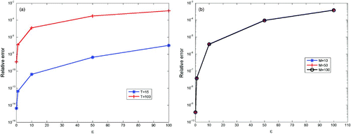
Table 1. Computational times on a personal computer of various simulations in 1D and 2D.

	2D	1D
T=15 days, dt=0.1	67 s	10.69 s
T=15 days, dt=0.01	1 h\ 42 min	11 min
T=100 days, dt=0.1	46 min	4.7 min

In Table 1 are given various computational times on a personal computer for the simulation in 2D and in 1D. The simulations were performed with the same parameters as in Figure 2 and for the 2D simulations we used and M=10 points of discretization of the boundary.

We observe that simulating in 1D improves greatly the computational times, especially for the large time simulations. Since the evolution of a cancer disease can be very slow, it is important to be able to simulate the model for large times (say, more than a year in the human case). Here the times are in days and we see that, thanks to the convergence of Theorem 3.3, the numerical method for simulating the model is improved in terms of the computational cost.

5. Conclusion

We proved the convergence of the family of the solutions to the problem (7), to the one of the problem (8), and established a simple expression for the limit in term of the solution of a 1D equation. This is of great importance in view of the applications since we can simulate only the 1D equation and thus highly improve the computational cost. The model is now ready to be a useful tool with two main possible applications.

First it can be used as a diagnostic tool, to refine the actual classifications like TNM (for Tumour, lymph Nodes and Metastases) or SBR (Scarff, Bloom, Richardson) which deal only with the visible metastases. Indeed, identifying the parameters m and α for a given patient could determine the metastatic aggressiveness of its cancer. A fundamental problem in this direction that needs to be addressed is the mathematical parameter identifiability (inverse problem). Efficient numerical methods have also to be developed to achieve practical parameter identification, which will permit us to confront the model to real data in order to study its validity as a phenomenological model.

The second main application of the model is its use in the rationalization of the temporal administration protocols for an anti-angiogenic drug alone as well as in combination with a cytotoxic drug. Finding the optimal schedule for these issues is still a clinical open question. The associated optimization problems through the model have to be solved both at theoretical and numerical levels.

References

- Barbolosi , D. , Benabdallah , A. , Hubert , F. and Verga , F. 2009 . Mathematical and numerical analysis for a model of growing metastatic tumors . Math. Biosci. , 218 : 1 – 14 .
- Barbolosi , D. and Iliadis , A. 2001 . Optimizing drug regimens in cancer chemotherapy: A simulation study using a PKPD model . Comput. Biol. Med. , 31 : 157 – 172 .
- Benzekry , S. 2010 . “ Mathematical and numerical analysis of a model for anti-angiogenic therapy in metastatic cancers ” . submitted for publication Available at http://hal.archives-ouvertes.fr/hal-00518110/fr/
- Benzekry , S. 2011 . Mathematical analysis of a two-dimensional population model of metastatic growth including angiogenesis . J. Evol. Equations , 11 : 187 – 213 .
- Billy , F. , Ribba , B. , Saut , O. , Morre-Trouilhet , H. , Colin , T. , Bresch , D. , Boissel , J. , Grenier , E. and Flandrois , J. 2009 . A pharmacologically based multiscale mathematical model of angiogenesis and its use in investigating the efficacy of a new cancer treatment strategy . J. Theoret. Biol. , 260 : 545 – 562 .
- Devys , A. , Goudon , T. and Laffitte , P. 2009 . A model describing the growth and the size distribution of multiple metastatic tumors . Discrete Contin. Dyn. Syst. Ser. , B 12 : 731 – 767 .
- d'Onofrio , A. and Gandolfi , A. 2004 . Tumour eradication by antiangiogenic therapy: Analysis and extensions of the model by Hahnfeldt et al. (1999) . Math. Biosci. , 191 : 159 – 184 .
- d'Onofrio , A. , Ledzewicz , U. , Maurer , H. and Schttler , H. 2009 . On optimal delivery of combination therapy for tumors . Math. Biosci. , 222 : 13 – 26 .
- Ebos , J. M.L. , Lee , C. R. , Cruz-Munoz , W. , Bjarnason , G. A. , Christensen , J. G. and Kerbel , R. S. 2009 . Accelerated metastasis after short-term treatment with a potent inhibitor of tumor angiogenesis . Cancer Cell , 15 : 232 – 239 .
- Folkman , J. 1972 . Antiangiogenesis: New concept for therapy of solid tumors . Ann. Surg. , 175 : 409 – 416 .
- Hahnfeldt , P. , Panigraphy , D. , Folkman , J. and Hlatky , L. 1999 . Tumor development under angiogenic signaling: A dynamical theory of tumor growth, treatment, response and postvascular dormancy . Cancer Res. , 59 : 4770 – 4775 .
- Harris , J. , Morrow , M. and Norton , L. 1997 . “ Malignant tumors of the breast ” . In Cancer: Principles and Practice of Oncology , 5 , Edited by: DeVita , J. V. , Hellman , S. and Rosenberg , S. 1557 – 1602 . Philadelphia : Lippincott-Raven .
- Hinow , P. , Gerlee , P. , McCawley , L. J. , Quaranta , V. , Ciobanu , M. , Wang , S. , Graham , J. M. , Ayati , B. P. , Claridge , J. , Swanson , K. R. , Loveless , M. and Anderson , A. R. 2009 . A spatial model of tumor-host interaction: Application of chemotherapy . Math. Biosci. Eng. , 6 : 521 – 545 .
- Iwata , K. , Kawasaki , K. and Shigesada , N. 2000 . A dynamical model for the growth and size distribution of multiple metastatic tumors . J. Theoret. Biol. , 203 : 177 – 186 .
- Paez-Ribes , M. , Allen , E. , Hudock , J. , Takeda , T. , Okuyama , H. , Vinals , F. , Inoue , M. , Bergers , G. , Hanahan , D. and Casanovas , O. 2009 . Antiangiogenic therapy elicits malignant progression of tumors to increased local invasion and distant metastasis . Cancer Cell , 15 : 220 – 231 .
- Perthame , B. 2007 . “ Transport Equations in Biology, Frontiers in Mathematics ” . Basel : Birkhaser .
- Riely , G. J. , Rizvi , N. A. , Kris , M. G. , Milton , D. T. , Solit , D. B. , Rosen , N. , Senturk , E. , Azzoli , C. G. , Brahmer , J. R. Sirotnak , F. M. 2009 . Randomized phase II study of pulse erlotinib before or after carboplatin and paclitaxel in current or former smokers with advanced non-small-cell lung cancer . J. Clin. Oncol. , 27 : 264 – 270 .
- Swan , G. W. 1990 . Applications of optimal control theory in biomedicine . Math. Biosc. , 101 : 237 – 284 .