Fatal disease and demographic Allee effect: population persistence and extinction

Abstract

If a healthy stable host population at the disease-free equilibrium is subject to the Allee effect, can a small number of infected individuals with a fatal disease cause the host population to go extinct? That is, does the Allee effect matter at high densities? To answer this question, we use a susceptible–infected epidemic model to obtain model parameters that lead to host population persistence (with or without infected individuals) and to host extinction. We prove that the presence of an Allee effect in host demographics matters even at large population densities. We show that a small perturbation to the disease-free equilibrium can eventually lead to host population extinction. In addition, we prove that additional deaths due to a fatal infectious disease effectively increase the Allee threshold of the host population demographics.

Keywords:

• Allee effect
• extinction
• persistence

1. Introduction

In population models, the Allee effect refers to inverse density dependence at low population sizes. A strong Allee effect occurs in these models when there is a positive equilibrium density, Allee threshold, and the species goes extinct whenever population densities fall below the threshold 1,7–11,13–15. The presence of a strong Allee effect in host demographics makes the population vulnerable to extinction as a fatal disease may tip it below the Allee threshold. In a recent paper, Hilker et al. 14 showed that in the presence of strong Allee effect in host demographics, a simple susceptible–infected (SI) epidemic model can exhibit stable periodic orbits (by Hopf bifurcation), multiple stationary states, and catastrophic collapses of endemic equilibria. Using a similar SI model with the strong Allee effect, Thieme et al. 16 established by mathematical theorems that the transition from population decline to population collapse is mediated by a Hopf bifurcation and a heteroclinic orbit. The SI models of Hilker et al. and Thieme et al. are structurally similar to predator–prey models that have an Allee effect in the prey population and a linear functional response (prey eaten per predator per unit time) 2 3 6 10,12–14,17 18. However, most of these studies on the interplay of Allee effects and infectious diseases, especially those in the conservation biology literature, seem to be largely concerned with the role of the Allee effect at small population densities 9.

In the present paper, we prove that the presence of an Allee effect in host demographics matters even at large population densities. That is, we show that a small perturbation to the disease-free equilibrium can eventually lead to host population extinction. We focus on the following question. If a healthy stable host population at the disease-free equilibrium is subject to an Allee effect, can a small number of infected individuals with a fatal disease cause the host population to go extinct? To answer this question, we use the SI epidemic model of Hilker et al. and obtain model parameters that lead to host population persistence (with or without infected individuals) and to host extinction. We note that in epidemiological models with frequency-dependent transmission and disease-related mortality, a small number of infected individuals can drive the host population to extinction. In these models, when the strong Allee effect is missing in the host demographics, the transition from host persistence to host extinction occurs ‘gradually’ or ‘slowly’ while the model parameters vary. However, in the presence of a strong Allee effect, the transition from host persistence to extinction is much more abrupt 12.

The paper is organized as follows. In Section 2, we introduce the SI model with the strong Allee effect in the demographic equation. In Section 3, we state conditions for population persistence (Theorem 3.3) and extinction (Theorem 3.5). Theorems 3.3 and 3.5 are proved in Sections 4 and 5, respectively. In Section 6, we use specific parameter regimes to illustrate regions of host population persistence (with or without infected individuals) and/or extinction. Section 7 is concerned with the stability of a unique endemic stationary point, and concluding remarks are presented in Section 8.

2. Model equations

To introduce the SI model of Hilker et al. 14 with a strong Allee effect in the host demographics, we let P=P(t)≥0 denote the host population at time t≥0. In the presence of an infectious disease, the total population

splits into susceptible (S) and infected (I) compartments. As in 14, to make the disease fatal, we assume that there is no recovery from it. The disease transmission is assumed to be density dependent by the mass action rate β SI, where β>0 is the incidence coefficient. There is no vertical transmission. The infected individuals reproduce into the susceptible class, and the per capita net growth function is split into

where b(P) is the fertility function and m(P) is the natural mortality. Since the disease is fatal, the infected individuals suffer an additional disease-induced mortality, which is represented by the constant virulence μ. The SI model is described by the following autonomous system of two differential equations.

As in 14, we specify the demographic functions and assume that a strong Allee effect in the host demographics is manifested by the following per capita net growth rate

where K is the carrying capacity, k is the Allee threshold (minimum viable density of the disease-free population) and 0<k<K. The parameter a (a>0) adjusts the maximum per capita growth rate. As shown in 14, the functional form of g can be obtained by assuming a density-dependent per capita mortality rate and a quadratic per capita fertility rate

The demographic function b(P) describes a population with increasing mortality where the number of encounters between the two sexes is proportional to P ² and a linearly decreasing offspring survival in crowded habitats. The demographic function m(P) describes a population with linearly increasing mortality rate and is introduced so that

The positive parameters e and c determine the effect of density dependence and independence in the demographic function, respectively, but they do not affect the per capita growth rate g(P). As in 14, e is chosen so that P≤K+k+e, which ensures that the fertility function b(P) is positive.

Following Hilker et al. 14, we non-dimensionalize the system (1) by the following change of variables:

In the new variables, Model (1) reduces to the following equations:

To simplify the notation, we drop the ‘prime’ on t′ so that Model (3) reduces to the system of equations

where

3. Statement of results

In Model (4), we take initial conditions

Theorem 3.1

The solution (p(t), i(t)) of Equations (4) and (5) satisfies the inequalities

Proof

Clearly, i(t)>0 and then also p(t)<1 for all t>0. To prove that i(t)<p(t) for all t>0, we assume, to the contrary, that there exists a point [ttilde] such that i(t)<p(t) for all 0<t<[ttilde] and . Then,

and by Model (4),

which is a contradiction since .   ▪

Model (4) has three disease-free equilibrium points:

Any solution of Model (4) with p(0)<u satisfies

and the host population goes extinct. In particular, (0, 0) is locally asymptotically stable. The equilibrium point (u, 0) is unstable since one of the eigenvalues of the Jacobian matrix at (u, 0) is the positive number r(1−u)u; the other eigenvalue, may be positive, negative, or zero.

If σ≤1, then by the second equation of Model (4)

and the infected population goes extinct. That is, σ≤1 implies disease extinction in Model (4). In the rest of the paper, we assume that σ>1.

As in 14, we introduce the critical host population density for disease establishment, the disease threshold,

and the basic reproductive ratio,

where P _T is the point at which the linear infecteds nullcline crosses the horizontal axis. Moreover, P _T>1 is equivalent to , and 0<P _T<1 is equivalent to

Theorem 3.2

If P _T>1, then (1, 0) is locally asymptotically stable and the disease goes extinct.

Indeed, in this case, the eigenvalues of the Jacobian matrix at (1, 0), −r(1−u) and , are both negative.

In the rest of the paper, we consider the case where 0<P _T<1. We first state conditions for persistence of the infected population of Model (4).

Theorem 3.3

If

and

then for any solution of Model (4) with for some there exists a δ>0 depending only on and a time such that

Remark 3.4 (a) Let

Then, Equation (8) reduces to

In Figure 1, we illustrate that condition (8) holds whenever the maximum value of f, f(y _cr ), is bigger than , where . (b) If (the first case), condition (8) reduces to

Figure 1. Condition (8) hold where u<y _cr <P _T and the horizontal line, i=((σ−1)/σ)(1−P _T), is below the maximum value of the p-nullcline, i=(r/α)(1−p)(p−u)p.

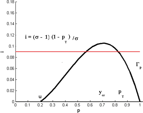
In Model (4), all trajectories (p(t), i(t)) with p(0)<u lead to host population extinction. When 0<P _T<1, Theorem 3.3 asserts that in the presence of disease infection, the Allee threshold is effectively increased to . That is, due to disease-induced death, the host population size needs to be larger to ensure persistence of the infected population 10.

In Model (4), host population extinction is possible with 0<P _T<1 and . To illustrate this, we next consider the case where instead of Equation (7), we have

Theorem 3.5

If and

for some sufficiently small then every solution of Model (4) with for any δ>0 sufficiently small and i(0)>0 satisfies

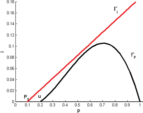
Condition (12) holds whenever the p-, Γ _p , is below the i-, Γ _i , of Model (4) (Figure 2).

Theorems 3.3 and 3.5 are proved in Sections 4 and 5, respectively. In Section 6, we give numerical examples and discuss the conclusion of these theorems in terms of persistence and extinction of a healthy population in which a small but fatal disease was introduced.

Figure 2. Condition (12) holds where P _T<u<1 and the p-nullcline is below the i-nullcline.

4. Proof of Theorem 3.3

To prove Theorem 3.3, we first establish two auxiliary results, Lemmas 4.1 and 4.2.

Lemma 4.1

Assume that 0<P _T<1. Then, for any there exists a small enough and a function such that if

then

Proof

We assume that

and derive a bound on T* in terms of , and i(0). We claim that

Indeed, otherwise there is a smallest t=[ttilde] such that , and then . But by Equations (4) and (14)

at t=[ttilde] if

which is a contradiction.

We next claim that

where and c is a constant. Indeed, at any point [tcirc], where , we have, by Equations (4), (13), and (14),

if

It follows that for some

Next, from Equation (4) for i and inequalities (13) and (14), we get

where , c ₁ is a positive constant, and . Hence,

if

It follows that for some [ttilde], where

Note that depends on i(0), if , then . Hence, the right-hand side of Equation (16) is actually a function , where if $i(0)\rightarrow 0$.   ▪

If in the above proof i(0) is equal to ϵ, then becomes a function which depends only on ϵ and . In the next lemma, we restate this case where instead of t=0 we take any initial time t=t ₁.

Lemma 4.2

Assume that 0<P _T<1 and

where ϵ is sufficiently small depending on . If for then

Proof

[Proof of Theorem 3.3] In view of Lemma 4.2, we need only to bound i(t) from below in intervals , where and t ₁>0. We may further assume that (t ₁, t ₂) is a maximal interval for which so that . Then, for some values t smaller than t ₁. Let t ₀ be the largest value of t, t<t ₀, with the property that i(t) is monotonically decreasing from t ₀ to t ₁. Then,

and

or by Model (4),

Hence, by Equation (7),

where

We claim that there exists an such that

Indeed, since , if the assertion (20) is not true, then there exists a such that

and therefore

or by Model (4),

Since, by Equations (17) and (18)

we get

But this is a contradiction to Equation (8) if we choose such that is the value at which the maximum is attained for the left-hand side of Equation (8). Consequently, with this chosen value of , we conclude that Equation (20) is satisfied, and in particular,

We can therefore apply Lemma 4.2 to deduce that

Note that the way was determined, may be viewed as a function (of ϵ only). We next observe that

where c ₀ is a positive constant. Hence,

This estimate applies to any interval t ₁<t<t ₂, where and . Combining this estimate with Lemma 4.1, it follows that i(t)>δ if .   ▪

5. Proof of Theorem 3.4

We denote by the union of

and the interval

and by the union of

and the interval

where Γ _i and Γ _p are, respectively, the i- and p-nullclines of Model (4).

Hence,

Consider first the case where

so that

lies strictly above

Hence,

It follows that, every trajectory of Model (4) must cross at some time, entering the region above (unless it is initially already above ), and thereafter it remains above so that and as .

Consider next the case when equality holds in Equation (12) with . Then, and have one point of intersection, , where they are tangent to each other. As easily computed, the eigenvalues λ _i of the Jacobian matrix at Q are λ₁=0 and . Hence, Q is a saddle point, so that no trajectory (p(t), i(t)) which is above , for some t=[ttilde], can converge to Q as . It follows, as illustrated in the phase diagram in Figure 3, that any trajectory (p(t), i(t)) with , where is sufficiently small and δ₂>0, must cross successively and and then, as in the case considered above, as . In particular, for some finite time t _δ.

Under the condition (12) with ϵ sufficiently small, the i-nullcline intersects the p-nullcline at two points Q ₁ and Q ₂, where and are small enough, so that, by continuity, the corresponding trajectory with , where , is sufficiently small and δ₂>0 satisfies , and hence as .

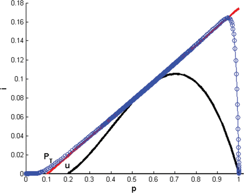
Remark 5.1 The assumption that ϵ in condition (12) is small is essential. Figure 4 shows an example where the two points of intersection of the nullclines, Q ₁ and Q ₂, are not sufficiently close, and in this case, the solution (p(t), i(t)) converges to Q ₂ as .

Figure 3. In Model (4), Γ _i (straight line) is tangent to Γ _p (cubic) and a solution (circles) with initial condition (1, 0.0001) converges to (0, 0) as t→∞. Here, α=r=0.016667, d=0.00482, σ=1.241, and u=0.2.

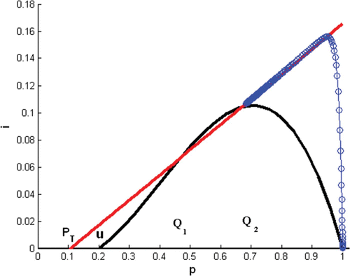
Figure 4. Phase plane of Model (4) with two interior positive steady points and a solution (circles) with initial condition (1, 0.0001) converges to an interior fixed point as t→∞. Here, α=r=0.016667, d=0.00482, σ=1.23, and u=0.2.

6. Extinction and persistence

We are interested in the following question regarding system (4). Given a healthy stable population with p(0)=1 but subject to the Allee effect in the host demographics, can a small number of individuals infected with a fatal disease cause the host population to go extinct? If this is the case no matter how small the initial number of infected individuals, i(0), then we say that the model parameters are in the host extinction phase; otherwise we say that the parameters are in the host persistence phase.

We shall, for illustration, focus on the parameters u, the Allee threshold, and the infection parameter σ, keeping all the other parameters fixed. When 0<P _T<1, under conditions (7) and (8), Theorem 3.3 asserts that if for some (and, in particular, if p(0)=1), for any small number of infected individuals i(0), the inequality (9) holds. Thus, (u, σ) is a point of persistence of the infected population and, hence (by Theorem 2.1), also of the host population. On the other hand, Theorem 3.5 asserts that (u, σ) is a point of host population extinction if and condition (12) holds.

We illustrate the regions of persistence versus extinction in Figure 5 in the case

The curve

is defined by P _T=1, that is, σ−1=A. The curve

is defined by u=P _T. The curve

is such that, with , equality holds in Equation (8); then, Equation (8) holds if . Finally, the curve

is such that, with , equality holds in Equation (12) with ; then, Equation (12) with holds if .

Figure 5. Region of host persistence with no infected individuals (disease extinction) is denoted by ‘open squares’, region of disease persistence is denoted by ‘open circles,’ and region of host extinction is denoted by ‘asterisks’ in (u, σ)-plane with initial condition (p, i)=(1, 0.0001). Here, α=0.1, d=0.25, r=0.2, u∈(0, 0.5), and σ>1.

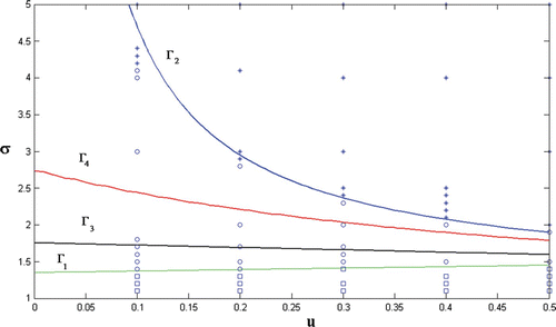
Theorem 3.3 asserts that the region between Γ₃ and Γ₂ is a region of persistence of the infected population. Theorem 3.5 asserts the region for some small η>0 is a region of extinction of the host population. Points in regions between Γ₁ and Γ₃ and between Γ₂ and Γ₄ may be either points of disease population extinction or persistence. Simulations in Figure 5 with initial condition show points of host population persistence without infected individuals by open squares, points of disease persistence by open circles, and points of host population extinction by asterisks. Note that by Theorem 3.2, every point below Γ₁ is a state of host population persistence with no infected individuals.

It follows from Figure 5 that if we increase the infection rate (respectively, the Allee threshold) while all the other parameters are kept fixed at their current values, then it is possible for the system parameters to shift from host population persistence phase to host population extinction phase. In Figure 5, stability questions (equilibrium versus oscillation) are not considered.

7. Stability of the unique endemic equilibrium

Let

Theorem 7.1

If 0<u<P _T<1, then Model (4) has a unique stationary point

and is locally asymptotically stable if

Proof

Note that is a stationary point with ī>0 if and only if is a zero of the function

This may only occur for x in the interval P _T< x<1. Since f (1)<0, f(P _T)>0, and if u<x<1, f(x) has precisely one zero in this interval. The slope of the i-nullcline at is clearly larger than the slope of the p-nullcline, that is,

The Jacobian matrix of Model (4) at is

and . Both eigenvalues of have negative real parts if

But these two inequalities are, respectively, inequalities (22) and (23).   ▪

Hilker et al. 14 showed that Model (4) is capable of exhibiting an interior periodic orbit via a Hopf bifurcation of the interior stationary points.

8. Conclusion

Many plant and animal species are known to exhibit the Allee effect 9. Examples of species that exhibit the Allee effect and suffer from fatal diseases include the endangered African wild dog Lycaon pictus 4 5 8 and the island fox Urocyon littoralis 1 7. Studies of systems that exhibit the Allee mechanism seem to be focused on the role of the Allee effect at small population densities. However, in combination with an infectious disease, we prove that a small perturbation to the disease-free equilibrium can lead to the catastrophic extinction of the host population. That is, a small number of infected individuals can lead to host population extinction. To prove this result, we use the relative position of a disease threshold to the Allee threshold and host population carrying capacity and obtained verifiable conditions that guarantee the persistence (with or without infected individuals) or extinction of the host population of the SI model of Hilker et al. 14. In the presence of the Allee effect in the host demographics, population models which exhibit multistability and transitions from host population persistence (with or without infected individuals) to extinction become much more abrupt. Mathematical proofs of these bifurcation phenomena and how they impact host population extinctions at high densities are open questions.

Also, we prove that when there is an Allee effect in the host demographics and a fatal disease invades the host population, then the Allee threshold is effectively increased. Deredec and Courchamp 10 reported a similar result. At large population densities, the Allee effect and infectious diseases can work together to drive otherwise stable healthy host populations to extinction even at large population densities. Thus, understanding the interplay between the Allee effect and disease epidemic models may have important implications in conservation biology, ecology, and epidemiology.

With view to the effects of migration on populations of endangered species, for example, the endangered African wild dog, it would be interesting to investigate how the extinction threshold of one population is influenced by the collective migrations of several populations with different Allee thresholds.

Acknowledgements

The authors thank the referees for useful comments and suggestions that improved our manuscript. This research has been supported in part by the Mathematical Biosciences Institute of The Ohio State University, Department of Homeland Security, DIMACS and CCICADA of Rutgers University, and the National Science Foundation under grant DMS 0931642 and 0832782.

References

- Angulo , E. , Roemer , G. W. , Berec , L. , Gascoigne , J. and Courchamp , F. 2007 . Double Allee effects and extinction in island fox . Conserv. Biol , 21 : 1082 – 1091 .
- Bazykin , A. 1998 . “ Nonlinear Dynamics of Interacting Populations ” . In World Scientific Series on Nonlinear Analysis: Series A , Vol. 22 , River Edge, NJ : World Scientific .
- Berezovsky , F. , Novozhilov , S. and Karev , G. 2007 . Population models with singular equilibrium . Math. Biosci , 208 : 270 – 299 .
- Burrows , R. , Hofer , H. and East , M. I. 1995 . Population dynamics, intervention and survival in African wild dogs (Lycaon pictus) . Proc. R. Soc. B Biol. Sci , 262 : 235 – 245 .
- Clifford , D. L. , Mazet , J. A.K. , Dubovi , E. J. , Garcelon , D. K. , Coonan , T. J. , Conrad , P. A. and Munson , L. 2006 . Pathogen exposure in island fox (Urocyon littoralis) populations: Implications for conservation management . Biol. Conserv , 131 : 230 – 243 .
- Conway , E. D. and Smoller , I. A. 1986 . Global analysis of a system of predator–prey equations . SIAM J. Appl. Math , 46 : 630 – 642 .
- Courchamp , F. , Clutton-Rock , T. and Grenfell , B. 1999 . Inverse density dependence and the Allee effect . Trends Ecol. Evol , 14 : 405 – 410 .
- Courchamp , F. , Clutton-Rock , T. and Grenfell , B. 2000 . Multipack dynamics and the Allee effect in the African wild dog, Lycaon pictus . Anim. Conserv , 3 : 277 – 285 .
- Courchamp , F. , Berec , L. and Gascoigne , J. 2008 . Allee Effect in Ecology and Conservation , New York : Oxford University Press .
- Deredec , A. and Courchamp , F. 2006 . Combined impacts of Allee effect and parasitism . Oikos , 112 : 667 – 679 .
- Franke , J. and Yakubu , A.-A. 2008 . Disease-induced mortality in density dependent discrete-time SIS epidemic models . J. Math. Biol , 57 ( 6 ) : 755 – 790 .
- Hilker , F. M. 2010 . Population collapse to extinction: The catastrophic combination of parasitism and Allee effect . J. Biol. Dyn , 4 : 86 – 101 .
- Hilker , F. M. , Langlais , M. , Petrovski , S. V. and Malchow , H. 2007 . A diffusive SI model with Allee effect and application to FIV . Math. Biosci , 206 : 61 – 80 .
- Hilker , F. M. , Langlais , M. and Malchow , H. 2009 . The Allee effect and infectious diseases: Extinction, multistability, and the (dis-)appearance of oscillations . Am. Nat , 173 ( 1 ) : 72 – 88 .
- Shreiber , S. J. 2009 . Allee effects, extinctions and chaotic transients in simple population models . Theor. Popul. Biol , 64 : 201 – 209 .
- Thieme , H. R. , Dhirasakdanon , T. , Han , Z. and Trevino , R. 2009 . Species decline and extinction: Synergy of infectious disease and Allee effect? . J. Biol. Dyn , 3 ( 2–3 ) : 305 – 323 .
- van Voorn , G. L.K. , Hemerik , L. , Boer , M. P. and Kooi , B. W. 2007 . Heteroclinic orbits indicate overexploitation in predator–prey systems with a strong Allee effect . Math. Biosci , 209 : 451 – 469 .
- Wang , J. , Shi , J. and Wei , J. 2011 . Predator–prey system with strong Allee effect in prey . J. Math. Biol , 62 : 291 – 331 .