A comparison of a deterministic and stochastic model for Hepatitis C with an isolation stage

Abstract

We formulate a deterministic epidemic model for the spread of Hepatitis C containing an acute, chronic and isolation class and analyse the effects of the isolation class on the transmission dynamics of the disease. We calculate the basic reproduction number R₀ and show that for R₀≤1, the disease-free equilibrium is globally asymptotically stable. In addition, it is shown that for a special case when R₀>1, the endemic equilibrium is locally asymptotically stable. Furthermore, an analogous stochastic epidemic model for Hepatitis C is formulated using a continuous time Markov chain. Numerical simulations are used to estimate the mean, variance and probability distributions of the discrete random variables and these are compared to the steady-state solutions of the deterministic model. Finally, the expected time to disease extinction is estimated for the stochastic model and the impact of isolation on the time to extinction is explored.

Keywords:

• epidemiology
• Hepatitis C
• deterministic model
• stochastic model

1. Introduction

Hepatitis C, formerly referred to as ‘non-A, non-B’ Hepatitis, is an infectious disease affecting the liver, caused by the Hepatitis C virus (HCV). Hepatitis C was first recognized as a separate disease in 1975 and its causative agent, HCV, was identified in 1989. The HCV is a small, enveloped, positive-sense single-stranded RNA virus of the family Flaviviridae [38]. Structurally, the virus consists of an RNA core surrounded by an icosahedral protein coat, which is further encased in a lipid envelope. Replication of the RNA-based virus involves the use of the enzyme RNA-dependent RNA polymerase that has a high error rate. Consequently, the virus mutates very rapidly and has no single genotype. Currently, there are 7 known genotypes and more than 100 different strains of HCV [37]. According to the World Health Organization, nearly 3% of the world's population is infected with HCV. It is estimated that more than 170 million people globally are infected with HCV, while nearly 350,000 people die worldwide as a result of Hepatitis C-related liver diseases each year [5].

HCV is primarily spread by blood-to-blood contact through blood transfusions, intravenous dug use (IDU) and the use of poorly sterilized medical equipment. Prior to the development of an effective blood screening test in 1990, the primary route of transmission of Hepatitis C in the developed world was blood transfusions [33]. Recently however, IDU has emerged as a major source of contracting HCV in the developed world [36]. On the other hand, in most parts of the developing world such as Egypt, Pakistan and India, HCV is still predominantly spread through blood transfusions and unsafe medical procedures. Other methods of transmission include vertical transmission from an infected mother to her child, the use of shared personal items such as razors and toothbrushes, and body piercing and tattooing which often involve the use of contaminated equipment and dyes. The possibility of transmission of HCV through sexual activity is still being debated [6,31,46].

Hepatitis C is characterized by an acute and a chronic stage. Initial infection by HCV results in acute Hepatitis C, which is largely asymptomatic. Only about 15% of cases display mild symptoms such as decreased appetite, fatigue, nausea, muscle or joint pains, and weight loss. The diagnosis of Hepatitis C is thus very difficult and consequently, the HCV epidemic is often called the ‘silent epidemic’ [8]. The initial infection resolves spontaneously in nearly 20% of cases [43]. About 80% of individuals exposed to HCV, however, eventually develop a chronic infection, which is characterized by the detection of HCV RNA for a period of at least six months after the original infection [36]. This stage of the disease can last for decades. Most people experience minimal or no symptoms during the first few years of the infection [43]. After several years of living with the disease, however, Hepatitis C becomes the primary cause of cirrhosis and liver cancer. Nearly 5–20% of chronic Hepatitis C patients develop cirrhosis over 30 years and 1–5% die from cirrhosis or liver cancer. Individuals who develop cirrhosis have a 20-fold greater risk of hepatocellular carcinoma, a rate of 13% per year. It is estimated that Hepatitis C is the cause of 27% of cirrhosis cases and 25% of hepatocellular carcinoma worldwide [13,18,23,26,42].

While treatment for Hepatitis C is possible, there is currently no known vaccine for the disease – due primarily to the rapid rate of mutation of HCV [12]. In general, chronically infected individuals are treated with a combination of interferon alpha and the antiviral drug ribavirin for a period of 24 or 48 weeks, depending on the HCV genotype. The response to treatment also varies by genotype and ranges from 70% to 80% for genotypes 2 and 3 to almost non-existent for genotype 6 [24,47]. Recovery from infection with HCV does not result in long-term immunity. Therefore, any model for Hepatitis C must take into account this lack of acquired immunity.

The existence of a chronic stage is an essential epidemiological feature of Hepatitis C. According to Chavez [32], however, relatively little deterministic analysis of diseases with a chronic stage has been done. Reade [39], for instance, has discussed an ordinary differential equations (ODE) model for infections with acute and chronic stages. His work focuses on the impact of vaccination on the model and uses mostly numerical simulations. Similarly, Lou [30] has performed a global analysis of a four-state ‘susceptible’, ‘exposed’, ‘acute’ and ‘chronic’ model and proven certain theorems regarding the stability of the steady states of the model. Other deterministic models pertinent to our work have also been proposed and analysed [9,10,20,23]. In addition, some epidemic models specifically for the spread of HCV have also been proposed. Chavez [32] has formulated an age-structured ODE model for Hepatitis C that contains both an acute and a chronic infection class with the force of infection modelled by proportionate mixing. Similarly, Dontwi [15] has considered the transmission of Hepatitis C through IDU in an acute, chronic and recovered model. Other deterministic epidemic models for the spread of HCV include those in [17,50].

Over the past few decades, several stochastic epidemic models for the spread of infectious diseases have also been proposed and analysed [2,4,7,40,45,48,49]. Allen [1,3] has explored the utility of stochastic epidemic models by comparing them with deterministic models. An important qualitative difference between deterministic and stochastic epidemic models in general is the asymptotic dynamics [1]. Furthermore, stochastic models also allow for the possibility of disease extinction in finite time and therefore the expected time to disease extinction can be calculated [1–3]. It is also observed that stochastic models better capture the uncertainty and variability that is inherent in real-life epidemics due to factors such as the unpredictability of person-to-person contact [3,44]. Despite the utility of stochastic models, however, very little stochastic modelling has been performed for HCV [34].

We will formulate a five-state ‘susceptible’, ‘acute’, ‘chronic’, ‘isolated’ and ‘recovered’ deterministic model and investigate the basic reproduction number R₀, and its effect on the existence and stability of the steady-state solutions of the deterministic model. Our model will extend the previous work done on modelling the spread of Hepatitis C in several key ways. Firstly, we will introduce a class and qualitatively assess the effect of this isolation class on the transmission dynamics of HCV. Quarantine of individuals suspected of being exposed to a disease, and the isolation of those with disease symptoms, constitute what is probably the first infection control measure since the beginning of recorded human history [21]. Over the decades, these control measures have been applied, with varying degrees of success, to combat the spread of some emerging and re-emerging diseases such as leprosy, plague, cholera, typhus, yellow fever, smallpox, diphtheria, tuberculosis, measles, Ebola, pandemic influenza and, more recently, severe acute respiratory syndrome [14,19,22,28,29,35]. However, almost no analysis of the effects of an isolation class on diseases with a chronic stage has been done and therefore, our paper will be one of the first attempts to study the effect of isolation on the spread of a disease with a chronic stage. Since Hepatitis C is largely asymptomatic, and chronically infected individuals can live for years without being identified, an isolation class can be used to consider individuals who have been clearly identified as being infected with HCV. Such individuals can then undergo treatment for HCV and take extra precautions while interacting with the people around them.

In addition, we will model the force of infection by a proportionate mixing, with the possibility of secondary infections due to contact with individuals who belong to the acute, chronic or isolation class. Furthermore, we will consider the disease-induced death rates for HCV in our model and will also take into account the possibility of recovery at every stage of the disease. These features will add to the complexity of our model and make it considerably more insightful from an epidemiological perspective than previous models [15,32].

Finally, we will construct an analogous stochastic version of our deterministic model using a continuous time Markov chain (CTMC) and compare the dynamics of both models. We will use numerical simulations to estimate the mean, variance and probability distributions of each discrete random variable and compare the results to the solutions of the corresponding deterministic model. Furthermore, we will use the stochastic model to analyse the effect of the isolation class on the mean time to disease extinction, which is important from an epidemiological viewpoint.

2. Deterministic model formulation

We will formulate a five-state model with individuals classified as susceptible, acute, chronic, isolated or recovered. Hepatitis C has an extremely slow progression that makes it difficult to characterize the natural history of the disease [11]. The following assumptions will therefore be made:

• (1) All infected individuals develop the acute form of Hepatitis C first.

• (2) Individuals with either the acute or chronic form of Hepatitis C or isolated individuals are capable of transmitting the disease.

• (3) Individuals with the acute form of the disease either progress to the chronic form or recover naturally. Since the acute form of the disease is largely asymptomatic, there is little chance of treatment at this stage.

• (4) Individuals chronically infected with Hepatitis C are either isolated or recover via treatment.

• (5) All isolated individuals will recover from the disease.

• (6) Individuals in the recovered class will over time become susceptible to the disease.

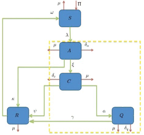
In addition, the model will assume that the susceptible population S has a constant recruitment rate Π and natural death rate μ. Susceptible individuals who get infected, suffer from the acute form of Hepatitis C and move to the state A with the force of infection given by λ. Individuals in A, in addition to the natural death rate μ, die at a disease-induced death rate δ_a. They also have a natural recovery rate of κ. Individuals with the acute form of the infection progress to the chronic form of the disease at a rate ξ, in which case the individual is shifted to state C. Individuals in C, in addition to the natural death rate μ, also die at a disease-induced death rate δ_c. Furthermore, these individuals recover at a rate ψ and thus move to the recovered state R. Also, the individuals in state C are isolated and moved to state Q at a rate α. Individuals in Q, in addition to the natural death rate μ, also die at a disease-induced death rate δ_q. Isolated individuals who recover from the disease move to recovered class at a rate γ. Finally, recovered patients in R become susceptible at a rate ω₁. The schematic diagram of our model is shown in (Figure 1).

Figure 1. Flow diagram of the model (1). The model consists of five sub-populations: susceptible S, acute A, chronic C, isolated Q and recovered R individuals.

Mathematically, the model is as follows:

where The description of variables and parameters of the model (1) are as follows:

Table

Variable	Description
N(t)	Total population
S(t)	Population of susceptible individuals
A(t)	Population of individuals with acute Hep-C
C(t)	Population of individuals with chronic Hep-C
Q(t)	Population of isolated individuals
R(t)	Population of recovered individuals

Table

Parameter	Description
Π	Recruitment rate
μ	Natural death rate
δa	Disease-induced death rate of individuals with acute Hep-C
δc	Disease-induced death rate of individuals with chronic Hep-C
δq	Disease-induced death rate of isolated individuals
γ	Recovery rate of isolated individuals
ξ	Progression rate from the acute to the chronic stage of Hepatitis C
α	Isolation rate of chronically infected individuals
κ	Natural recovery rate of acutely infected individuals
ψ	Recovery rate of chronically infected individuals
ω	Rate of loss of infection-acquired immunity
β	Effective contact rate
η	Modification parameter for infectiousness of acute individuals
ζ	Modification parameter for infectiousness of isolated individuals

Since Equation (1) is a model for human populations, all the associated parameters are non-negative. Furthermore, the following non-negativity result holds.

Theorem 2.1

The variables of the model (1) are non-negative for all time t>0. In other words, solutions of the system (1) with positive initial data will remain positive for all t>0.

Proof Let . Thus, t₁>0. It follows from the first equation of the model (1) that which can be rewritten as Hence, so that Similarly, it can be shown that A>0, C>0, Q>0, R>0 for all t>0.

We now prove a useful lemma.

lemma 2.2

The closed set is positively invariant.

Proof Adding all the equations of the model (1) gives

It follows that if . Thus, a standard comparison theorem can be used to show that . In particular, if . Thus, the region D is positively invariant.

Furthermore, if , then either the solution enters D in finite time, or N(t) approaches Π/μ asymptotically. Hence, the region D attracts all solutions in R₊⁵ and our solutions remain bounded.

Since the region D is positively invariant, it is sufficient to consider the dynamics of the flow generated by the model (1) in region D, where the usual existence and uniqueness results hold for the system.

2.1 Stability of disease-free equilibrium

In this section, we discuss the existence and stability of the disease-free equilibrium (DFE).

2.1.1 Local stability

The model (1) has a DFE, obtained by setting the right-hand sides of the equations in Equation (1) to zero, given by The local stability of ℵ₀ will be determined using the next generation operator method described in [16]. The non-negative matrix F, of the new infection terms, and the M-matrix, V, of the transition terms associated with the model (1) are given by and The eigenvalues of the matrix FV⁻¹ are It follows that the basic reproduction number is given by where The basic reproduction number measures the average number of new infections generated by a single infectious individual in a susceptible population. The reproduction number R₀ obtained above can be intuitively interpreted as follows. Susceptible individuals acquire infection following contact with either an acute (A), chronic (C) or isolated (Q) individual. The number of infections produced by an acutely infected individual (near the DFE) is given by the product of the infection rate of an acute (A) individual (β η) and the average duration in the acute (A) class (1/k₁). Furthermore, the number of infections produced by a chronically infected individual (near the DFE) is given by the product of the infection rate of a chronic (C) individual (β), the average duration in the chronic (C) class (1/k₂) and the probability that an acute (A) individual survives and progresses to the chronic C stage ξ/k₁. Similarly, the number of infections produced by an isolated individual (near the DFE) is given by the product of the infection rate of an isolated (Q) individual (β ζ), the average duration in the isolation (Q) class (1/k₂) and the probability that an acute (A) individual survives and progresses to the isolation Q stage . Thus, the average number of new infections generated by a single infectious individual is given by The local stability of the DFE holds due to Theorem 2 of [16].

lemma 2.3

The DFE, ℵ₀, of the model (1) is locally asymptotically stable if R₀<1 and unstable if R₀>1.

Lemma 2.3 implies that, for R₀<1, a small influx of infectious individuals will not lead to a large outbreak of the disease. To ensure that disease elimination is independent of the initial sizes of sub-populations, however, it is necessary to show that the DFE is globally asymptotically stable if R₀<1. This is explored below.

2.1.2 Global stability

Theorem 2.4

The DFE of the model (1), given by Equation (3), is globally asymptotically stable whenever R₀≤1.

Proof A comparison theorem will be used for the proof. The equations for the infected components of the model (1) can be written as These equations can be simplified as follows:

where F and V are as defined previously.

Lemma 2.3 established the local asymptotic stability of the DFE when R₀<1, or equivalently, 1. This is equivalent to the statement that all eigenvalues of F−V have negative real parts when R₀<1 [16]. Therefore, the linearized differential inequality system (3) is stable whenever R₀<1. Consequently, by a standard comparison theorem, we have

Substituting A=C=Q=0 in the model (1) gives Therefore, and hence, the DFE ℵ₀ is globally asymptotically stable whenever R₀≤1.

The epidemiological implication of the above result is that Hepatitis C can be eliminated from the population if the basic reproduction number R₀ can be brought down to and maintained at a value less than unity. Therefore, the condition R₀<1 is a necessary and sufficient condition for disease elimination.

2.2 Existence and stability of endemic equilibrium

In this section, the existence of endemic equilibria of the model (1) will be discussed. We define endemic equilibria to be those fixed points of the system (1) in which at least one of the infected sub-populations A, C or Q of the model is non-zero.

2.2.1 Existence of endemic equilibrium

Let denote an arbitrary endemic equilibrium of the model (1) so that Solving the equations of the model (1) at steady state gives

where Consider S**. Then, using Equations (3) and (4) Note that if C**=0, then and we obtain the DFE solution. Thus, we may assume that C**¬=0. Therefore,

where

Finally, using Equation (4), the endemic steady states are given by

We have therefore established the following result.

lemma 2.5

The model (1) has endemic equilibria, of the form ℵ₁, given by Equation (7), whenever R₀>1

2.2.2 Local stability of endemic equilibrium

We have established the existence of endemic equilibria ℵ₁. We now consider the local stability of the endemic equilibrium for a special case, where the disease-induced death rates are assumed to be negligible and are set to zero. Under this setting, with , the rate of change of the total population is given by Hence, as . Therefore, for the purpose of our analysis, we will take , where N* is the total population at the DFE.

Theorem 2.6

The unique endemic equilibrium of the model at N=N* is locally asymptotically stable if R₀>1.

Proof It can easily be shown that, with N=N*, the model has a unique endemic equilibrium, denoted by . We will employ Krasnoselskii's sub-linearity method [27,41] to prove that the endemic equilibrium is locally asymptotically stable.

Let R₀>1 and N=N* (to ensure the endemic equilibrium exists). Furthermore, the substitution is used to reduce the model to

The reduced model's endemic equilibrium is equivalent to the original endemic equilibrium under the substitution done above.

Linearizing the reduced system (8) around the ℵ₁ gives

where

It follows that the Jacobian of the system (9) evaluated at ℵ₁ is

Now assume that the system (9) has a solution of the form

where Substituting a solution of the form (11) into the system (9) yields

The system (12) is now simplified as follows. First, all the negative terms in the bottom three equations of Equation (12) are moved to the respective left-hand sides. The resulting three equations are then rewritten in terms of Z₁ and substituted into the first equation of Equation (12). Finally, all negative terms in the first equation are moved to the left-hand side. Thus,

where with The notation ( denotes the ith coordinate of the vector . Here, , and the matrix M has non-negative entries. It is now easy to verify that endemic equilibrium satisfies

If is a solution of Equation (12), then by Krasnoselskii's result it is possible to find a minimal positive real number r such that

where with lexicographic order and |·| is a norm in C. The main goal is to show that .

Assume now that the and consider the following two cases.

Case 1: ω=0. In this case, Equation (12) is a homogeneous linear system in the variables . The determinant of this system is given by where

Now, Equation (5) implies that at endemic equilibrium, we have . Hence, This means that system (12) has unique solution which corresponds to the DFE (ℵ₀) of the model (1).

Case 2: . Since Re(ω)>0 (by assumption), then >1 for i=1, 2, 3, 4. Denote F(ω) = min . Then, F(ω) >1 and . Furthermore, by the minimality of r, we have

Taking the norm on both sides of the equations in Equation (13) and noting that M is a non-negative matrix, it follows that Therefore,

Now, Equation (17) contradicts Equation (16). Therefore, .

Thus, all eigenvalues of the characteristic equation associated with the linearized system (9) will have negative real parts. Therefore, the unique endemic equilibrium , equivalent to ℵ₁, is locally asymptotically stable whenever R₀>1.

The epidemiological implication of the above result is that Hepatitis C will remain endemic in the population for R₀>1 provided that the initial population contains a sufficient number of infected individuals.

3. Stochastic model formulation

We now formulate an analogous stochastic model using a CTMC. Our purpose will be to explore the dynamics of this stochastic model and to compare them with the dynamics from the corresponding deterministic model. An important qualitative difference between deterministic and stochastic epidemic models in general is the asymptotic dynamics. Eventually, stochastic solutions (sample paths) converge to the disease-free state irrespective of the value of the basic reproduction number R₀ even though the corresponding deterministic solution converges to an endemic equilibrium [2]. Furthermore, stochastic models also allow for the possibility of disease extinction in finite time and therefore the expected time to disease extinction can be calculated [1,2]. It is also observed that stochastic models better capture the uncertainty and variability that is inherent in real-life epidemics due to factors such as the unpredictability of person-to-person contact [44].

3.1 Model formulation and the infinitesimal state probabilities

Following [3], we assume the total population size to be bounded. We denote the bound by K. Let , , , and denote discrete random variables for the number of individuals in the susceptible, acute, chronic, isolation and recovered classes, respectively. Furthermore, let The continuous-time stochastic dynamical system is a multivariate process with a joint probability function

where We further assume that the stochastic process is time homogeneous. Thus, using the notation of [1], and therefore, the probability of transition from the state (s, a, c, q, r) to the state is defined by

where

In order for the probabilities to be meaningful (non-negative and bounded by 1), the following is assumed: Since all the parameters are positive, a small value of Δ t ensures that the above condition is satisfied.

Although we now have the infinitesimal transition probabilities in hand, it is difficult to express the transition matrix and the generator matrix in easily expressible forms. One possible solution to this problem is given in [2] and we will make use of this in a later section. Our stochastic model has five independent discrete random variables and it is therefore even more cumbersome to express the associated transition and generator matrices. We therefore desist from this exercise.

We now assume that the stochastic process satisfies the Markov property: Using the Markov property and the infinitesimal transition probabilities, we can express the state probabilities at time t+Δ t in terms of the state probabilities at time t. For the sake of simplicity, we assume that the total population at time t is less than the upper bound K and furthermore that none of the random variables is zero. The purpose of these two assumptions is to ignore numerous tedious sub-cases.

Proposition 3.1

Assume . Further assume that none of the variables s, a, c, q, r is zero. Then, the state probabilities satisfy the following difference equations: where

The remaining cases, which result from removing the previous assumptions, are straightforward to calculate.

Some properties of the Markov chain can now be discussed. The chain is reducible, consisting of at least two communication classes [1], given by D:={(s, 0, 0, 0, 0) where and where . Furthermore, E is not closed since . On the other hand D is closed since and .

Since E is an open class all states in E are transient. Hence, and in view of D being the only closed communication class, all sample paths will eventually be absorbed into the communication class D. However, while D is indeed a closed class, it does not contain an absorbing state since .

In view of the above discussion, the following theorem is established.

Theorem 3.2

The CTMC is reducible with at least two communication classes. There are no absorbing states. However, all sample paths are eventually absorbed in the closed class D:={(s, 0, 0, 0, 0) where .

The two communication classes D and E correspond to the disease-free and endemic stages of the disease, respectively. Therefore, the above result indicates that every sample path is eventually absorbed into the disease-free class and therefore, irrespective of parameter values the stochastic model will always converge to a disease-free state. This is in direct contrast to the deterministic case in which an endemic steady-state solution always exists for R₀>1. Thus, the deterministic case allows for the possibility of the disease having an endemic equilibrium, depending on the value of a threshold parameter, while the stochastic model always predicts an eventual DFE. Furthermore, disease extinction takes place in finite time in the stochastic case while in the deterministic case a DFE is only approached asymptotically. Depending on the value of R₀, however, the sample paths for the stochastic model might remain in the endemic class E for a very long time. In fact numerical simulations of the stochastic model for values of the basic reproduction number R₀ greater than unity suggest the existence of a quasi-endemic equilibrium. As a consequence, for practical purposes, the stochastic model follows closely the behaviour of the corresponding deterministic model for moderate periods of time. This will be explored further in the section on numerical simulations.

3.2 The Kolmogorov differential equations

In order to further investigate the time evolution of , an attempt can be made to form the Kolmogorov differential equations. In this section, we form the forward equation. The process for obtaining the backward equation is similar. For the sake of simplicity we will assume that the total population at time t is less than the upper bound K. We will further assume that none of the random variables is zero at time t.

Theorem 3.3

Assume and . Further assume that is a differentiable function of time. Then, the Kolmogorov forward equation for the stochastic process is given by

Proof We have assumed that and We can therefore make use of the preceding difference equations. Noting the fact that , the forward equation is obtained by taking the following limit

The Kolmogorov forward equation for our model is a difference-differential equation in several variables. Ideally, a solution of this equation would give us a complete picture of the time evolution of the joint probability distribution . This will then enable us to calculate the moments of each discrete random variable. This is equivalent to obtaining exact solutions of the corresponding deterministic model (1).

In order to solve the Kolmogorov forward equation, we will attempt to express it in matrix form. Following [25], let p(t) denote the probability vector containing the state probabilities. Thus, The corresponding generator matrix Q(t), using the notation of [1], can be constructed using the infinitesimal transition probabilities and is given by where .

The forward Kolmogorov equation in matrix form is now given by

Equation (20) can now be solved using numerical methods such as matrix exponentiation or a finite differences scheme [25]. However, the use of such numerical techniques requires truncating both p(t) and Q(t). We therefore, impose the following bound on the total population With this bound, p(t) and Q are reduced to finite matrices with dimensions based on the value of the bound N. Specifically, p(t) will be a vector of length , while Q will be a square matrix of dimension .

It is apparent that increasing the value of the bound N greatly increases the complexity and size of the generator matrix Q, which results in computational difficulties. In fact, even for values as small as N=20, the size of the generator matrix Q makes numerical computation practically impossible. As a result, even though an algorithm for the numerical solution of Equation (20) can be written, it is not possible to actually solve Equation (20), except for very small values of the bound N. We mention, however, that numerical computation will be greatly simplified if the number of classes in the model is reduced. Thus, for a stochastic SIR model, for example, it is possible to obtain a numerical solution for the Kolmogorov equation for values of N as large as 100 [25].

We have solved Equation (20) for the case N=12. For this value of N, Q is a square matrix of dimension 6, 188×6, 188. The solution of Equation (20) can be used to calculate the probability distribution of each discrete random variable as a function of time and state space.

4. Numerical simulations

For the purpose of numerical simulations, we will formulate our stochastic model as a discrete time Markov chain (DTMC) and employ a constant time step Δ t. This simplifies many of the numerical simulations and allows us to calculate the numerical mean, which is not possible when using a CTMC with random inter-event times. As mentioned in [2], if the time step Δ t is small enough, the DTMC provides an excellent approximation to the original formulation of the stochastic model as CTMC.

4.1 Simulations for the deterministic model

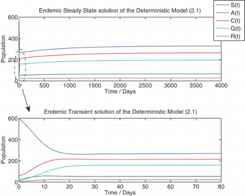
We solve the deterministic model (1) numerically for the two qualitatively different cases, R₀<1 and R₀>1, which correspond to the disease-free and endemic equilibria, respectively (Figures 2 and 3).

Figure 2. Numerical solution of the deterministic model (1) at {R₀=0.6453}. Initial population:

Π=0.12; γ=0.18; κ=0.2; ω=0.95;

ξ=0.7; α=0.15; ψ=0.05; δ_a=0.000233; δ_c=0.00233; δ_q=0.001667; η=0.5; ζ=0.1; β=0.1369.

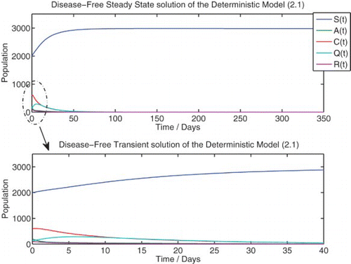
Figure 3. Numerical solution of the deterministic model (1) at {R₀=2.6889}. Initial population: (

(0),

(0),

(0),

(0),

(0))=(600, 20, 60, 12, 10). Π=1; γ=0.18; κ=0.2; ω=0.95;

ξ=0.7; α=0.15; ψ=0.05; δ_a=0.000233; δ_c=0.00233; δ_q=0.001667; η=0.5; ζ=0.1; β=0.5703.

We observe that the numerical simulation agrees with the theoretical result that predicts a globally asymptotically stable DFE for R₀≤1. Despite the initial condition containing a large number of infected individuals, the solution of the deterministic system approaches the DFE. The numerical steady-state value of the susceptible population agrees with the theoretical result of Π/μ.

Here too, we observe that the numerical simulation agrees with the theoretical result that predicts a locally asymptotically stable endemic equilibrium for R₀>1. In addition, the steady-state values of the simulation also agree with the theoretical steady-state values. We observe that the steady-state solution predicts a population that contains a large number of individuals with chronic infection as well as a significant number of isolated individuals.

4.2 The dependence of R₀ on state parameters

We analyse the dependence of R₀ on α, γ and β, which denote the isolation rate of chronically infected individuals, the recovery rate of isolated individuals and the effective contact rate, respectively. This will result in a better understanding of the effects of isolation on the dynamics of our model. The results are plotted as three-dimensional graphs and contour plots.

Figure 4(a) and 4(b) illustrates the dependence of the basic reproduction number R₀ on α, which is the isolation rate of chronically infected individuals and γ, which is the recovery rate of isolation individuals. The plot suggests that increasing either α or γ decreases the basic reproduction number R₀. Therefore, for the above values of the other state parameters, the isolation of chronically infected individuals can help bring down and maintain R₀ at a value less than unity, thereby resulting in a DFE for the model (1). The epidemiological implication of this is that, for the above values of the other state parameters, Hepatitis C can be eliminated from a population over time, if the rate of isolation of chronically infected individuals or the rate of recovery of the isolated individuals is increased.

Figure 4. The dependence of R₀ on some state variables. (a) The contour plot of R₀ as a function of α and γ, (b) R₀ as a function of α and γ, (c) the contour plot of R₀ as a function of α and β and (d) R₀ as a function of α and β. Π=10; γ=0.1; κ=0.7535; ω=0.95;

ξ=0.8; α=0.2; ψ=0.05; δ_a=0.000233; δ_c=0.00233; δ_q=0.001667; η=0.5; ζ=0.1; β=0.3.

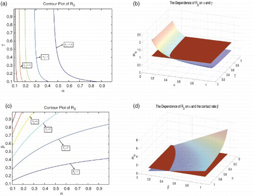
Similarly, Figure 4(c) and 4(d) illustrate the dependence of the basic reproduction number R₀ on α and β, which is the effective contact rate. The plot suggests that increasing α decreases the basic reproduction number R₀ and can help maintain it at a value less than unity, provided that the effective contact rate is not too large. This suggests that isolation can be pursued as an effective public health control mechanism only when the effective contact rate is sufficiently small.

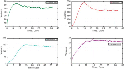
4.3 Numerical mean and variance of each discrete random variable

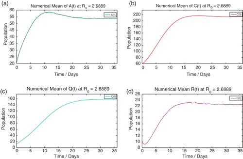
We numerically simulate 10,000 sample paths to estimate the mean and variance of each discrete random variable , , and . The results are shown below. We observe that there is excellent agreement with the solutions to the corresponding deterministic case. Very slight divergences are a consequence of the properties of the moments of the joint probability distribution and the moment closure problem (Figures 5–7).

Figure 5. Comparison of the solution to the deterministic model (1) and the numerical means of each discrete random variable from the stochastic model at R₀=2.6889.

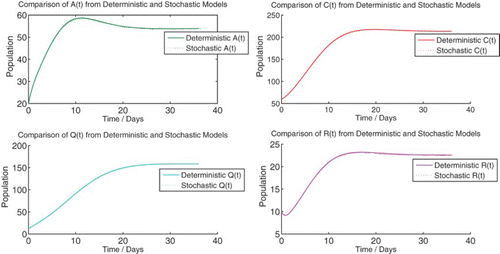
Figure 6. The numerical mean of each discrete random variable calculated using 10,000 sample paths. Numerical mean of the discrete random variables (a)

(t), (b)

(t), (c)

(t) and (d)

(t). Initial population: (

(0),

(0),

(0),

(0),

(0))=(600, 20, 60, 12, 10). Π=1; γ=0.18; κ=0.2; ω=0.95;

ξ=0.7; α=0.15; ψ=0.05; δ_a=0.000233; δ_c=0.00233; δ_q=0.001667; η=0.5; ζ=0.1; β=0.5703.

Figure 7. The variance of each discrete random variable calculated using 10,000 sample paths: (a)

(t), (b)

(t), (c)

(t) and (d)

(t).

4.4 Probability distributions

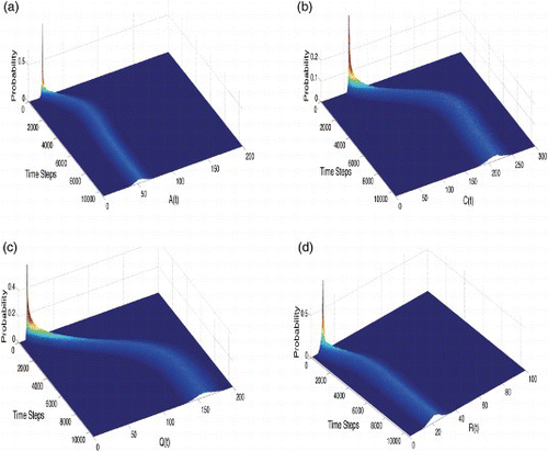
We compile results from 5000 sample paths to numerically estimate the probability distribution associated with each discrete random variable from the stochastic model as a function of time and state space. We observe that the stationary probability distributions follow a path similar to the steady-state solution of the corresponding deterministic case. This is the source of the strong agreement of the numerical mean of each discrete random variable from the stochastic model with the numerical solutions of the corresponding deterministic model (1). The initial spike in probability is due to fixed initial conditions being taken in each stochastic realization of the model (Figure 8).

Figure 8. The probability distribution of each discrete random variable calculated using 5000 sample paths. (a) Probability distribution of

(t) at {R₀=2.6889}, (b) probability distribution of

(t) at {R₀=2.6889}, (c) probability distribution of

(t) at {R₀=2.6889} and (d) probability distribution of

(t) at {R₀=2.6889}. Initial population: (

(0),

(0),

(0),

(0),

(0))=(600, 20, 60, 12, 10). Π=1; γ=0.18; κ=0.2; ω=0.95;

ξ=0.7; α=0.15; ψ=0.05; δ_a=0.000233; δ_c=0.00233; δ_q=0.001667; η=0.5; ζ=0.1; β=0.5703.

4.5 Mean time to extinction

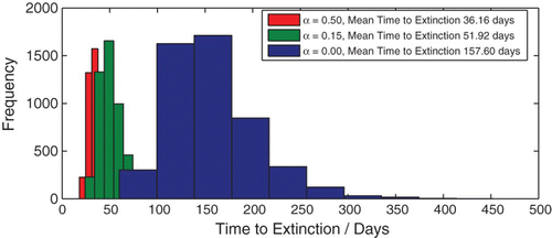
A simple consequence of the stochastic formulation of our model is a finite time to disease extinction. We use Monte Carlo simulations to analyse the effect of an isolation class on this mean time to disease extinction. We first consider the case of the threshold quantity R₀ being less than unity. We have, therefore, used a value of R₀ less than unity; 5000 stochastic realizations of the model were executed to construct histograms showing the distribution of the mean extinction time for two cases; one in which the rate of isolation of chronic individuals is 15% and the other in which the rate of isolation is 50%. We observe that all other parameters being constant, increasing the rate of isolation of chronic individuals leads to a considerable decrease in the mean time to disease extinction (Figure 9).

Figure 9. Mean time to disease extinction plotted as a histogram for three cases: α=0, α=0.15 and α=0.5. Initial population: (

(0),

(0),

(0),

(0),

(0))=(600, 20, 60, 10, 10). Π=1; γ=0.2; κ=0.2; ω=0.95;

ξ=0.8; ψ=0.05; δ_a=0.000233; δ_c=0.00233; δ_q=0.001667; η=0.5; ζ=0.1; β=0.1880; Δ t=0.0069.

In addition, we also perform numerical simulations to analyse the mean time to extinction for values of R₀ slightly greater than but very close to unity. Note that the deterministic model (1) predicts that for values of R₀ greater than unity, the DFE is locally asymptotically unstable and therefore Hepatitis C should persist in the population. However, simulations of the stochastic model indicate a finite mean time to disease extinction even for values of R₀ greater than unity. We execute 5000 stochastic simulations to construct histograms showing the distribution of the mean extinction time for two cases; one in which the rate of isolation of chronic individuals is 15% and the other in which the rate of isolation is 50%. The plots are given in Figure 10. In both cases, the effective contact rate β is adjusted so as to result in a value of R₀=1.01. The following initial conditions were used.

Figure 10. The mean time to disease extinction for two cases in which the basic reproduction number R₀ is slightly greater than unity computed using 5000 stochastic simulations each. Mean time to disease extinction for the cases (a) β=0.439,α=0.50 and R₀=1.01 and (b) β=0.213,α=0.15 and R₀=1.01. Initial population: (

(0),

(0),

(0),

(0),

(0))=(600, 20, 60, 10, 10). Π=1; γ=0.2; κ=0.2; ω=0.95;

ξ=0.8; ψ=0.05; δ_a=0.000233; δ_c=0.00233; δ_q=0.001667; η=0.5; ζ=0.1; Δ t=0.0069.

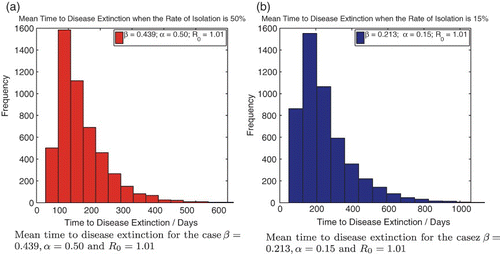
The mean time to extinction when the isolation rate is 15% is 255.24 days, while the mean time to extinction when the isolation rate is 50% is 142.03 days. Thus, despite the basic reproduction number R₀ being the same in both cases, we observe that increasing the rate of isolation decreases the mean time to disease extinction, even when the effective contact rate β is moderately high. We therefore conclude that increasing the rate of isolation of chronically infected individuals can help reduce the mean time to disease extinction for Hepatitis C.

5. Discussion

A deterministic epidemic model for the spread of Hepatitis C, which incorporates the possibility of a isolation state, is formulated. Global analysis of the equilibrium solution is performed. The existence of a DFE and an endemic equilibrium is shown. It is further demonstrated that the DFE is globally asymptotically stable for values of the basic reproduction number R₀<1. Therefore, Hepatitis C can be entirely eliminated from the population if and only if R₀<1. Furthermore, it is proven, for a special case, using a sub-linearity trick that the endemic equilibrium is locally asymptotically stable for R₀<1. Thus, analysis of the model (1) suggests that if R₀>1, Hepatitis C will persist in the population, provided that there are a sufficient number of infectious individuals in the population. It is also shown that numerical simulations of the deterministic model agree with the theoretical results. Finally, the dependence of the basic reproduction number R₀ on the state parameters and β is explored. In particular, it is observed that increasing the rate of isolation of chronically infected individuals α can lower the value of R₀ to less than unity, and hence, produce a DFE, provided that the effective contact rate β is sufficiently small. Thus, from an epidemiological perspective, increasing the rate of isolation of chronically infected individuals can, under some circumstances, help eliminate Hepatitis C from the population.

A corresponding stochastic model for the spread of HCV, in the form of a CTMC, is also constructed. It is shown that the stochastic model exhibits broadly the same behaviour as the deterministic model except that it associates a positive probability to disease extinction regardless of the value of R₀. It should be noted, however, that disease extinction for the case R₀>1 takes exceedingly long and this fact is demonstrated by the numerical simulations. The numerical mean, variance and probability distribution of each discrete random variable is calculated using Monte Carlo simulations. It is found that the numerically calculated means and probability distributions are in excellent agreement with the corresponding results from the deterministic case. Finally, the effect of increasing the rate of isolation of chronically infected individuals on the mean time to disease extinction is investigated using numerical simulations. It is observed that the mean time to extinction decreases as the rate of isolation is increased. Thus, it is concluded that increasing the rate of isolation of chronically infected individuals can help reduce the duration of a Hepatitis C epidemic.

REFERENCES

- L.J.S. Allen, An Introduction to Stochastic Processes with Applications to Biology, 2nd ed., Chapman and Hall/CRC, Boca Raton, FL, 2003.
- L.J.S. Allen, An introduction to stochastic epidemic models, in Mathematical Epidemiology, F. Brauer, P. Van den Driessche, and J. Wu, eds., Springer-Verlag, Berlin, 2008, pp. 77–128.
- L.J.S. Allen and A.M. Burgin, Comparison of deterministic and stochastic SIS and SIR models in discrete time, Math. Biosci. 163 (2000), pp. 1–33. doi: 10.1016/S0025-5564(99)00047-4
- L.J.S. Allen, D.A. Flores, R.K. Ratnayake, and J.R. Herbold, Discrete-time deterministic and stochastic models for the spread of rabies, Appl. Math. Comput. 132 (2002), pp. 271–292. doi: 10.1016/S0096-3003(01)00192-8
- M.J. Alter, Hepatitis C: The clinical spectrum of the disease, NIH Consensus Development Conference on Management of Hepatitis C, Bethesda, MD, 1997.
- M.J. Alter, Prevention of spread of hepatitis C, Hepatology 36 (2002), pp. 93–98. doi: 10.1002/hep.1840360712
- N. Bailey, A simple stochastic epidemic, Biometrika 37 (1950), pp. 193–202
- U. Bandy, Hepatitis C virus (HCV): A silent epidemic, Med. Health R. I. 82 (1999), pp. 223–224.
- S. Busenberg and P. van den Driessche, Analysis of a disease transmission model in a population with varying size, J. Math. Biol. 28 (1990), pp. 257–270. doi: 10.1007/BF00178776
- S. Busenberg and K. Hadeler, Demography and epidemics, Math. Biosci. 101 (1990), pp. 63–74. doi: 10.1016/0025-5564(90)90102-5
- S.L. Chen and T.R. Morgan, The natural history of hepatitis C virus (HCV) infection, Int. J. Med. Sci. 3 (2006), pp. 47–52. doi: 10.7150/ijms.3.47
- R. Colina, C. Azambuja, R. Uriarte, C. Mogdasy, and J. Cristina, Evidence of increasing diversification of Hepatitis C viruses, J. Gen. Virol. 80 (1999), pp. 1377–1382.
- A.M. Di Bisceglie, S.E. Order, J.L. Klein, J.G. Waggoner, M.H. Sjogren, G. Kuo, and J.H. Hoofnagle, The role of chronic viral hepatitis in hepatocellular carcinoma in the United States, Am. J. Gastroenterol. 86 (1991), pp. 335–338.
- C.A. Donnelly, A.C. Ghani, G.M. Leung, A.J. Hedley, C. Fraser, S. Riley, and R.M. Anderson, Epidemiological determinants of spread of causal agent of severe acute respiratory syndrome in Hong Kong, Lancet 361 (2003), pp. 1761–1766. doi: 10.1016/S0140-6736(03)13410-1
- I.K. Dontwi, N.K. Frempong, D.E. Bentil, I. Adetunde, and E. Owusu-Ansah, Mathematical modeling of Hepatitis C Virus transmission among injecting drug users and the impact of vaccination, Amer. J. Sci. Ind. Res. 1 (2010), pp. 41–46.
- P. van den Driessche and J. Watmough, Reproduction numbers and sub-threshold endemic equilibria for compartmental models of disease transmission, Math. Biosci. 180 (2002), pp. 29–48. doi: 10.1016/S0025-5564(02)00108-6
- N. Esposito and C. Rossi, A nested-epidemic model for the spread of hepatitis C among injecting drug users, Math. Biosci. 188 (2004), pp. 29–45. doi: 10.1016/j.mbs.2003.11.001
- G. Fattovich, G. Giustina, F. Degos, F. Tremolada, G. Diodati, P. Almasio, and G. Realdi, Morbidity and mortality in compensated cirrhosis type C: A retrospective follow-up study of 384 patients, Gastroenterology 112 (1997), pp. 463–472. doi: 10.1053/gast.1997.v112.pm9024300
- A.B. Gumel, S. Ruan, T. Day, J. Watmough, F. Brauer, P. van den Driessche, and B.M. Sahai, Modelling strategies for controlling SARS outbreaks, Proc. R. Soc. Ser. B 271 (2003), pp. 2223–2232. doi: 10.1098/rspb.2004.2800
- K. Hadeler and C. Castillo-Chavez, A core group model for disease transmission, Math. Biosci. 128 (1995), pp. 41–45. doi: 10.1016/0025-5564(94)00066-9
- H.W. Hethcote, The mathematics of infectious diseases, SIAM Rev. 42 (2000), pp. 599–653. doi: 10.1137/S0036144500371907
- H.W. Hethcote, M. Zhien, and L. Shengbing, Effects of quarantine in six endemic models for infectious diseases, Math. Biosci. 180 (2002), pp. 141–160. doi: 10.1016/S0025-5564(02)00111-6
- Y. Hutin, M.E. Kitler, G.J. Dore, J.F. Perz, G.L. Armstrong, G. Dusheiko, and D. Lavanchy, Global burden of disease (GBD) for hepatitis C, J. Clin. Pharmacol. 44 (2004), pp. 20–29. doi: 10.1177/0091270003258669
- J.A. Ilyas and J.M. Vierling, An overview of emerging therapies for the treatment of chronic hepatitis C, Clin. Liver Dis. 15 (2011), pp. 515–536. doi: 10.1016/j.cld.2011.05.002
- A.J. Keeling and J.V. Ross, On methods for studying stochastic disease dynamics, J. R. Soc. Interface 5 (2008), pp. 171–181. doi: 10.1098/rsif.2007.1106
- K. Kiyosawa, T. Sodeyama, E. Tanaka, Y. Gibo, K. Yoshizawa, Y. Nakano, and H.J. Alter, Interrelationship of blood transfusion, non-A, non-B hepatitis and hepatocellular carcinoma: Analysis by detection of antibody to hepatitis C virus, Hepatology 12 (1990), pp. 671–675. doi: 10.1002/hep.1840120409
- M.A. Krasnoselskii, Positive Solutions of Operator Equations, Noordhoff Leyden, Groningen, 1964.
- M. Lipsitch, T. Cohen, B. Cooper, J.M. Robins, S. Ma, L. James, and M. Murray, Transmission dynamics and control of severe acute respiratory syndrome, Science 300 (2003), pp. 1966–1970. doi: 10.1126/science.1086616
- J.O. Lloyd-Smith, A.P. Galvani, and W.M. Getz, Curtailing transmission of severe acute respiratory syndrome within a community and its hospital, Proc. R. Soc. Lond. Ser. B Biol. Sci. 170 (2003), pp. 1979–1989. doi: 10.1098/rspb.2003.2481
- F. Luo and Z. Xiang, Global analysis of an endemic model with acute and chronic stages, Int. Math. Forum 7 (2012), pp. 75–81.
- A. Maheshwari and P.J. Thuluvath, Management of acute hepatitis C, Clin. Liver Dis. 14 (2010), pp. 169–176. doi: 10.1016/j.cld.2009.11.007
- M. Martcheva and C. Castillo-Chavez, Diseases with chronic stage in a population with varying size, Math. Biosci. 182 (2003), pp. 1–25. doi: 10.1016/S0025-5564(02)00184-0
- J. Marx, R. Hockberger, and R. Walls, Rosen's Emergency Medicine – Concepts and Clinical Practice, 7th ed., Mosby/Elsevier, Philadelphia, PA, 2010.
- D. Mather and N. Crofts, A computer model of the spread of hepatitis C virus among injecting drug users, Eur. J. Epidemiol. 15 (1999), pp. 5–10. doi: 10.1023/A:1007548307196
- R.G. McLeod, J.F. Brewster, A.B. Gumel, and D.A. Slonowsky, Sensitivity and uncertainty analyses for a SARS model with time-varying inputs and outputs, Math. Biosci. Eng. 3 (2006), pp. 527–544. doi: 10.3934/mbe.2006.3.527
- P.K. Nelson, B.M. Mathers, B. Cowie, H. Hagan, D. Des Jarlais, D. Horyniak, and L. Degenhardt, Global epidemiology of hepatitis B and hepatitis C in people who inject drugs: Results of systematic reviews, Lancet 378 (2011), pp. 571–583. doi: 10.1016/S0140-6736(11)61097-0
- R. Purcell, Hepatitis C virus: An introduction, NIH Consensus Development Conference on Management of Hepatitis C, Bethesda, MD, 1997.
- S.C. Ray and D.L. Thomas, Chapter 154: Hepatitis C, in Mandell, Douglas, and Bennett's Principles and Practice of Infectious Diseases, 7th ed., G.L. Mandell, J.E. Bennett, and R. Dolin, eds., Churchill Livingstone, Philadelphia, PA, 2009.
- B, Reade, R.G. Bowers, M. Begon, and R. Gaskell, A model of disease and vaccination for infections with acute and chronic phases, J. Theor. Biol. 190 (1998), pp. 355–367. doi: 10.1006/jtbi.1997.0557
- S. Riley, Large-scale spatial-transmission models of infectious disease, Science 316 (2007), pp. 1298–1301. doi: 10.1126/science.1134695
- M.A. Safi and A.B. Gumel, Global asymptotic dynamics of a model for quarantine and isolation, Discret Contin. Dyn. Syst. 14 (2010), pp. 209–231. doi: 10.3934/dcdsb.2010.14.209
- L.B. Seeff, Z. Buskell-Bales, E.C. Wright, S.J. Durako, H.J. Alter, F.L. Iber, and C.G. Hollingsworth, Long-term mortality after transfusion-associated non-A, non-B hepatitis, New Engl. J. Med. 327 (1992), pp. 1906–1911. doi: 10.1056/NEJM199212313272703
- M.L. Shiffman, Chronic Hepatitis C Virus: Advances in Treatment, Promise for the Future, Springer, New York, 2011.
- S. Spencer, Stochastic epidemic models for emerging diseases, Ph.D. diss., University of Nottingham, 2008.
- J.H. Tien and D.J. Earn, Multiple transmission pathways and disease dynamics in a waterborne pathogen model, Bull. Math. Biol. 72 (2010), pp. 1506–1533. doi: 10.1007/s11538-010-9507-6
- R.A. Tohme and S.D. Holmberg, Is sexual contact a major mode of hepatitis C virus transmission, Hepatology 52 (2010), pp. 1497–1505. doi: 10.1002/hep.23808
- J. Torresi, D. Johnson, and H. Wedemeyer, Progress in the development of preventive and therapeutic vaccines for hepatitis C virus, J. Hepatol. 54 (2011), pp. 1273–1285. doi: 10.1016/j.jhep.2010.09.040
- A.R. Tuite, J. Tien, M. Eisenberg, D.J. Earn, J. Ma, and D.N. Fisman, Cholera epidemic in Haiti, 2010: Using a transmission model to explain spatial spread of disease and identify optimal control interventions, Ann. Intern. Med. 154 (2011), pp. 593–601.
- G.H. Weiss, and M. Dishon, On the asymptotic behavior of the stochastic and deterministic models of an epidemic, Math. Biosci. 11 (1971), pp. 261–265. doi: 10.1016/0025-5564(71)90087-3
- S. Zhang and Y. Zhou, Dynamics and application of an epidemiological model for hepatitis C, Math. Comput. Model. 56 (2012), pp. 36–42. doi: 10.1016/j.mcm.2011.11.081