An optimal control problem for ovine brucellosis with culling

Abstract

A mathematical model is used to study the dynamics of ovine brucellosis when transmitted directly from infected individual, through contact with a contaminated environment or vertically through mother to child. The model developed by Aïnseba et al. [A model for ovine brucellosis incorporating direct and indirect transmission, J. Biol. Dyn. 4 (2010), pp. 2–11. Available at http://www.math.u-bordeaux1.fr/∼pmagal100p/papers/BBM-JBD09.pdf. Accessed 3 July 2012] was modified to include culling and then used to determine important parameters in the spread of human brucellosis using sensitivity analysis. An optimal control analysis was performed on the model to determine the best way to control such as a disease in the population. Three time-dependent controls to prevent exposure, cull the infected and reduce environmental transmission were used to set up to minimize infection at a minimum cost.

Keywords:

• ovine brucellosis
• optimal control
• sensitivity analysis
• population dynamics

Mathematics Subject Classification:

• 49J15
• 92B05
• 93A30

1. Introduction

Brucellosis is believed to be an ancient disease that was described more than 2000 years ago by the Romans [16]. It is one of the world's most widespread zoonoses [6,34,35] caused by infection with the bacterial genus Brucella. Brucellosis is a systemic, fever-producing infection caused by any of four species of Brucella bacteria: Brucella suis from pigs, Brucella melitensis from sheep, Brucella abortus from cattle, and Brucella canis, from dogs [37]. B. melitensis and arbotus have the highest pathogenicity of the four types and can be transmitted to humans [26]. These organisms, which are small aerobic intracellular coccobacilli, localize in the reproductive organs of host animals, causing abortions and sterility. They are shed in large numbers in the animal's urine, milk, placental, and other fluids. Exposure to infected animals and their products causes brucellosis in humans [18,28]. The rather non-specific signs of brucellosis may, in sub-Saharan Africa, lead to difficulty in distinguishing the disease clinically from typhoid, rheumatic fever, joint diseases, malaria and other conditions causing pyrexia [13,21,24,30]. Bruce first isolated B. melitensis in 1887 and has since then emerged in many parts of the world. Brucellosis still persists today in the developing nations of Africa, West Asia and some regions of Latin America [18,23].

The global burden of human brucellosis remains enormous and causes more than 500,000 infections per year worldwide [16]. The role that pathogens play in structuring ecological communities needs to be examined from both a theoretical and empirical perspective [9]. An effective control of animal brucellosis requires surveillance to identify infected animal herds, prevention of transmission to non-infected animal herds, and elimination of the sources of infection in order to protect vulnerable animals or herds coupled with measures to prevent re-introduction of the disease. The initial aim of surveillance and control programmes is the reduction of infection in the animal populations to reduce the effect of the disease on animal health and production, thus minimizing its impact on human health [27]. In areas where a brucellosis-free status has been established or where such a status is assumed from epidemiological data, the risk of importing the disease by means of animal movement must be eliminated [36]. Culling is the process of removing breeding animals from a group based on specific criteria. This is done either to reinforce certain desirable characteristics or to remove certain undesirable characteristics from the group. For livestock and wildlife alike, culling usually implies the killing of the removed animals. This method is not usually employed because it is nearly impossible to control Brucella by culling, without reimbursement of farmers for their financial losses due to removal of infected animals [17]. It would be beneficial to compare the costs associated with culling to the total loss of revenue without culling.

Several researchers have modelled the dynamics of brucellosis [2,7,15,25,29]. A model for ovine brucellosis was designed by Aïnseba et al. [1] incorporating direct, indirect, and vertical transmission. It is similar to other SI models used to describe aspects of the population dynamics of brucellosis with these modes of transmission. Almeida and Louza [3], constructed a simple mathematical model of brucellosis in Portuguese dairy herds. Dobson and Meargher [9] modelled its ecology and epidemiology in Yellowstone National Park in the USA. Mathematical models have for long been used to study disease dynamics at cellular and population levels. In this paper, the model by Aïnseba et al. [1] is modified to include culling of the infected subjects. Stability, sensitivity and optimal control analyses are carried out to determine the best way to control brucellosis.

2. Model formulation and analysis

A mathematical model developed by Aïnseba et al. [1] is modified to include culling of the infected subjects. As in their model, transmission is considered to be through three mechanisms which include vertical, direct or indirect. Vertical transmission is from mother to offspring. Direct transmission is through contact with an infected individual. Lastly, indirect transmission is through contact with a contaminated environment. The ovine population at any time t is divided into susceptible $S\left(t\right)$ and infected individuals $I\left(t\right)$. The proportion of the contaminated environment is denoted by $C\left(t\right)$. Let the per capita birth and death rates be b and d, respectively. It is assumed that $0<d\le b$ [32]. Let a proportion p of the newborns from infected mothers be infected. Therefore, the proportion that is susceptible at birth is $(1-p).$ Direct transmission is due to contact with susceptible $S\left(t\right)$ and infected $I\left(t\right)$ at a rate β. It is assumed that the process of direct transmission follows the mass action law and therefore denoted by $\beta SI$. Indirect transmission is between contaminated environment $C\left(t\right)$ and susceptible individuals $S\left(t\right)$. If α is the rate of infection then $\alpha SC$ is the force of infection from contaminated environment to susceptible subjects which is also modelled by mass action law. Infected subjects contaminate the environment at a rate η before being removed by culling at rate γ. The production of contaminant in the environment is given by $\eta (1-C)I$, and this is dependent on the remaining proportion of non-contaminated environment $(1-C)$. The environment gets rid of the contaminant at a rate δ. The flux diagram for the described dynamics is shown in Figure 1, and the parameters and values are given in Table 1.

Figure 1. Schematic representation of the model. Note that all rates are dependent on the variable for the group from which they originate (Colour online).

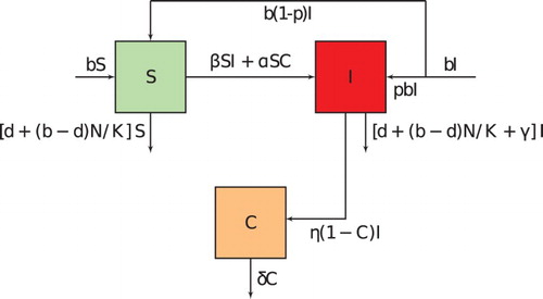
Table 1. Parameter values for ovine brucellosis and their descriptions.

Variable	Description	Dimensions
S:	Number of susceptible subjects
I:	Number of infectious subjects
C:	Proportion of contaminated environment
Parameter	Description	Value per year	Source
b	Per capita birth rate	0.83 births/per subject	[1]
d	Per capita mortality rate	0.79 deaths/subject	[1]
γ	Percentage culling rate	Estimated, $[0,1]$
K	Carrying capacity	1.82 $\times {10}^7$ subjects	[1]
p	Probability of vertical transmission	0.05	[1]
β	Direct transmission	Estimated
α	Indirect transmission	Estimated
η	Contamination rate	Estimated
δ	Disinfection rate	1.82 virus particles	[1]

From Figure 1, parameter descriptions and assumptions, the following model is obtained: (1) $\begin{array}{rl}\frac{\mathrm{d}S}{\mathrm{d}t}& =bS+(1-p)bI-\left(d+\frac{b-d}{K}N\right)S-\beta SI-\alpha SC,\\ \frac{\mathrm{d}I}{\mathrm{d}t}& =pbI-\left(d+\frac{b-d}{K}N\right)I+\beta SI+\alpha SC-\gamma I,\\ \frac{\mathrm{d}C}{\mathrm{d}t}& =\eta (1-C)I-\delta C,\end{array}$(1) where $N=S+I$ is the total population. Adding the first two expressions of Equation (1(1) $\begin{array}{rl}\frac{\mathrm{d}S}{\mathrm{d}t}& =bS+(1-p)bI-\left(d+\frac{b-d}{K}N\right)S-\beta SI-\alpha SC,\\ \frac{\mathrm{d}I}{\mathrm{d}t}& =pbI-\left(d+\frac{b-d}{K}N\right)I+\beta SI+\alpha SC-\gamma I,\\ \frac{\mathrm{d}C}{\mathrm{d}t}& =\eta (1-C)I-\delta C,\end{array}$(1) ), gives (2) $\frac{\mathrm{d}N}{\mathrm{d}t}=(b-d)N\left(1-\frac{N}{K}\right)-\gamma I,$(2) where K is the carrying capacity. Let us assume from the logistic equation (2(2) $\frac{\mathrm{d}N}{\mathrm{d}t}=(b-d)N\left(1-\frac{N}{K}\right)-\gamma I,$(2) ) that $N\left(t\right)=K,\mathrm{\forall }t\ge 0$. This simplifies system (1(1) $\begin{array}{rl}\frac{\mathrm{d}S}{\mathrm{d}t}& =bS+(1-p)bI-\left(d+\frac{b-d}{K}N\right)S-\beta SI-\alpha SC,\\ \frac{\mathrm{d}I}{\mathrm{d}t}& =pbI-\left(d+\frac{b-d}{K}N\right)I+\beta SI+\alpha SC-\gamma I,\\ \frac{\mathrm{d}C}{\mathrm{d}t}& =\eta (1-C)I-\delta C,\end{array}$(1) ) by replacing $S\left(t\right)$ with $K-I$ in the second equation ($\mathrm{d}I/\mathrm{d}t$ equation of Equation (1(1) $\begin{array}{rl}\frac{\mathrm{d}S}{\mathrm{d}t}& =bS+(1-p)bI-\left(d+\frac{b-d}{K}N\right)S-\beta SI-\alpha SC,\\ \frac{\mathrm{d}I}{\mathrm{d}t}& =pbI-\left(d+\frac{b-d}{K}N\right)I+\beta SI+\alpha SC-\gamma I,\\ \frac{\mathrm{d}C}{\mathrm{d}t}& =\eta (1-C)I-\delta C,\end{array}$(1) )) to remain with two equations, one for the infectives and the other for the contaminated environment. The systems then reduces to (3) $\begin{array}{r}\begin{array}{rl}\frac{\mathrm{d}I}{\mathrm{d}t}& =-(1-p)bI+\beta (K-I)I+\alpha (K-I)C-\gamma I,\\ \frac{\mathrm{d}C}{\mathrm{d}t}& =\eta (1-C)I-\delta C.\end{array}\end{array}$(3) Considering $i\left(t\right)=I\left(t\right)/K$ to be the fraction of the infected individuals in the community, then Equation (3(3) $\begin{array}{r}\begin{array}{rl}\frac{\mathrm{d}I}{\mathrm{d}t}& =-(1-p)bI+\beta (K-I)I+\alpha (K-I)C-\gamma I,\\ \frac{\mathrm{d}C}{\mathrm{d}t}& =\eta (1-C)I-\delta C.\end{array}\end{array}$(3) ) simplifies to (4) $\begin{array}{r}\begin{array}{rl}\frac{\mathrm{d}i}{\mathrm{d}t}& =-(1-p)bi+\beta K(1-i)i+\alpha (1-i)C-\gamma i,\\ \frac{\mathrm{d}C}{\mathrm{d}t}& =\eta K(1-C)i-\delta C.\end{array}\end{array}$(4) The model in Equation (4(4) $\begin{array}{r}\begin{array}{rl}\frac{\mathrm{d}i}{\mathrm{d}t}& =-(1-p)bi+\beta K(1-i)i+\alpha (1-i)C-\gamma i,\\ \frac{\mathrm{d}C}{\mathrm{d}t}& =\eta K(1-C)i-\delta C.\end{array}\end{array}$(4) ) will be analysed for stability and other important parameters for disease spread.

2.1. Equilibrium and stability analysis

From Equation (4(4) $\begin{array}{r}\begin{array}{rl}\frac{\mathrm{d}i}{\mathrm{d}t}& =-(1-p)bi+\beta K(1-i)i+\alpha (1-i)C-\gamma i,\\ \frac{\mathrm{d}C}{\mathrm{d}t}& =\eta K(1-C)i-\delta C.\end{array}\end{array}$(4) ) it can be noted that (0,0) is an equilibrium state. Therefore, the disease-free equilibrium state is given by $E_{\ast }\left(0\right)=(0,0).$ To obtain the endemic equilibrium point, let us assume fast dynamics in the environment and set the left-hand side of Equation (4(4) $\begin{array}{r}\begin{array}{rl}\frac{\mathrm{d}i}{\mathrm{d}t}& =-(1-p)bi+\beta K(1-i)i+\alpha (1-i)C-\gamma i,\\ \frac{\mathrm{d}C}{\mathrm{d}t}& =\eta K(1-C)i-\delta C.\end{array}\end{array}$(4) ) to zero to give (5) $C^{\ast }=\frac{\eta K{i}^{\ast }}{\eta K{i}^{\ast }+\delta },$(5) which is strictly positive since $i^{\ast }\in (0,1]$. Substituting for $C^{\ast }$ from Equation (5(5) $C^{\ast }=\frac{\eta K{i}^{\ast }}{\eta K{i}^{\ast }+\delta },$(5) ) into the first expression (i.e. the $\mathrm{d}I/\mathrm{d}t$ equation) of Equation (4(4) $\begin{array}{r}\begin{array}{rl}\frac{\mathrm{d}i}{\mathrm{d}t}& =-(1-p)bi+\beta K(1-i)i+\alpha (1-i)C-\gamma i,\\ \frac{\mathrm{d}C}{\mathrm{d}t}& =\eta K(1-C)i-\delta C.\end{array}\end{array}$(4) ) leads to (6) $\left[\right(1-p)b+\gamma ]i^{\ast }=\left(\beta K(1-i^{\ast })+\alpha (1-i^{\ast })\frac{\eta K}{\eta K{i}^{\ast }+\delta }\right)i^{\ast }.$(6)

This gives one solution as $i^{\ast }=0,$ which is the disease-free equilibrium point. Simplifying Equation (6(6) $\left[\right(1-p)b+\gamma ]i^{\ast }=\left(\beta K(1-i^{\ast })+\alpha (1-i^{\ast })\frac{\eta K}{\eta K{i}^{\ast }+\delta }\right)i^{\ast }.$(6) ) gives (7) $i^{\ast 2}-\left[1-\frac{\delta }{\eta K}-\frac{\alpha }{\beta K}-\frac{(1-p)b+\gamma }{\beta K}\right]i^{\ast }-\left[\frac{\delta }{\eta K}+\frac{\alpha }{\beta K}-\frac{\left(\right(1-p)b+\gamma )\delta }{\beta \eta K^2}\right]=0.$(7) Solving this equation gives two roots. One is negative and biologically meaningless, and a positive root given by (8) $i^{\ast }=\frac{1}{2}\left\{{\phi }^{\ast }+\sqrt{{\phi }^{\ast 2}+4\left[\frac{\delta }{\eta K}+\frac{\alpha }{\beta K}-\frac{\left(\right(1-p)b+\gamma )\delta }{\beta \eta K^2}\right]}\right\},$(8) where ${\phi }^{\ast }=1-\delta /\eta K-\alpha /\beta K-(1-p)b+\gamma /\beta K$. This is the point at which the disease has stabilized within the population.

The Jacobian of Equation (4(4) $\begin{array}{r}\begin{array}{rl}\frac{\mathrm{d}i}{\mathrm{d}t}& =-(1-p)bi+\beta K(1-i)i+\alpha (1-i)C-\gamma i,\\ \frac{\mathrm{d}C}{\mathrm{d}t}& =\eta K(1-C)i-\delta C.\end{array}\end{array}$(4) ) at steady state is given by (9) $J_{\ast }=\left[\begin{array}{cc}-(1-p)b-\gamma +\beta K-2\beta K{i}^{\ast }-\alpha C^{\ast }& \alpha (1-i^{\ast })\\ \eta K(1-C^{\ast })& -\eta K{i}^{\ast }-\delta \end{array}\right].$(9) To determine the prevalence of infection during the initial stages of the disease, the eigenvalues of Jacobian in Equation (9(9) $J_{\ast }=\left[\begin{array}{cc}-(1-p)b-\gamma +\beta K-2\beta K{i}^{\ast }-\alpha C^{\ast }& \alpha (1-i^{\ast })\\ \eta K(1-C^{\ast })& -\eta K{i}^{\ast }-\delta \end{array}\right].$(9) ) at the disease-free equilibrium are examined. The Jacobian matrix at $E_{\ast }\left(0\right)$ is given by (10) $J_{\ast }\left(0\right)=\left[\begin{array}{cc}-(1-p)b-\gamma +\beta K& \alpha \\ \eta K& -\delta \end{array}\right].$(10) From the Jacobian in Equation (10(10) $J_{\ast }\left(0\right)=\left[\begin{array}{cc}-(1-p)b-\gamma +\beta K& \alpha \\ \eta K& -\delta \end{array}\right].$(10) ), stability of the disease-free state ($E_{\ast }\left(0\right)$) is determined. Observe $E_{\ast }\left(0\right)$ is feasible if the trace is negative and determinant positive. Note from the Jacobian that the trace is negative if (11) $\beta K<(1-p)b+\gamma +\delta .$(11) Note that the right-hand side of Equation (11(11) $\beta K<(1-p)b+\gamma +\delta .$(11) ) is greater than 1 since $\delta >1;$ (see Table 1). At the beginning of infection, considering one infected subject introduced into a population of susceptibles, then $\beta \approx 1/N,$ where N is the initial population size. This implies that $\beta K\le 1$ (since $N\ge K$), and since $\delta >1,$ then $\beta K<(1-p)b+\gamma +\delta$. Thus, the trace of Jacobian (10(10) $J_{\ast }\left(0\right)=\left[\begin{array}{cc}-(1-p)b-\gamma +\beta K& \alpha \\ \eta K& -\delta \end{array}\right].$(10) ) is negative.

Further the determinant must be greater than zero to prove stability of this point. The determinant is given by $\frac{\beta K}{(1-p)b+\gamma }+\frac{\alpha \eta K}{\delta \left[\right(1-p)b+\gamma ]}<1\Rightarrow {\mathcal{R}}_0<1,$ where (12) ${\mathcal{R}}_0=\underset{\mathrm{Direct}\mathrm{transmission}}{\underbrace{\frac{\beta K}{(1-p)b+\gamma }}}+\underset{\mathrm{Indirect}\mathrm{transmission}}{\underbrace{\frac{\alpha \eta K}{\delta \left[\right(1-p)b+\gamma ]}}}.$(12) The basic reproduction number, ${\mathcal{R}}_0$, is the number of new infections that will result from one infective subject when introduced into a completely susceptible population [10]. The expression of ${\mathcal{R}}_0$ has two terms, one for direct and the other for indirect transmission of the disease during the culling process of the infected. This number gives us an insight on how fast the disease is spreading. ${\mathcal{R}}_0<1$ means that on average, an infected individual causes less than one new infected individual over the course of the infectious period and ${\mathcal{R}}_0>1$ implies that an infected individual produces more than one new infection. Therefore, the disease will die out when ${\mathcal{R}}_0<1$ and it will invade the population and persist when ${\mathcal{R}}_0>1$. Thus, the disease-free state is stable if ${\mathcal{R}}_0<1,$ and unstable otherwise. When ${\mathcal{R}}_0>1,$ an endemic equilibrium exists.

2.2. Sensitivity analysis of the model

The sensitivity indices of the reproductive number to the parameters in the model are calculated to find out how crucial each parameter is to disease transmission and prevalence. Sensitivity analysis is commonly used to determine the robustness of model predictions to parameter values since there are errors in data collection and the presumed parameter values. In this study, it is used to discover parameters that have a high impact on ${\mathcal{R}}_0$ and should be targeted by intervention strategies. Sensitivity indices allow us to measure the relative change in a state variable when a parameter changes. The normalized forward sensitivity index of a variable to a parameter is the ratio of the relative change in the variable to the relative change in the parameter [8]. When the variable is a differentiable function of the parameter, the sensitivity index may be alternatively defined using partial derivatives. In determining how best to reduce mortality and morbidity due to brucellosis, it is necessary to know the relative importance of the different factors responsible for its transmission and prevalence. Initial disease transmission is directly related to the basic reproduction number, ${\mathcal{R}}_0$, and disease prevalence is directly related to the endemic equilibrium point, specifically to the magnitudes of $i^{\ast }$ and $C^{\ast }$. These variables are relevant to the infectious subjects and the contaminated environment. $i^{\ast }$ is especially important because it represents those who are ill from brucellosis and is directly related to the total number of deaths. This section presents the assessment of the magnitude and direction of change inherent in the model as captured by the terms which define ${\mathcal{R}}_0.$ The sensitivity indices of the model parameters are computed using the approach in Chitnis et al. [8].

For our model, the baseline values used are summarized here and their values taken from the literature where possible. Some parameters are fixed in order to investigate several scenarios. For example, all newborns from an infected mother are infected at birth, but 95% of them recover after a short time [14]. We therefore neglect this short time and assume that 95% of the newborns are susceptible. The probability of vertical transmission p is therefore set to between 0 % and 5%. Using explicitly the formula in Equation (12(12) ${\mathcal{R}}_0=\underset{\mathrm{Direct}\mathrm{transmission}}{\underbrace{\frac{\beta K}{(1-p)b+\gamma }}}+\underset{\mathrm{Indirect}\mathrm{transmission}}{\underbrace{\frac{\alpha \eta K}{\delta \left[\right(1-p)b+\gamma ]}}}.$(12) ), an analytical expression for the sensitivity of ${\mathcal{R}}_0$ is equivalent to ${\mathrm{{\rm Y}}}_j^{{\mathcal{R}}_0}=\mathrm{\partial }{\mathcal{R}}_0/\mathrm{\partial }j\times j/{\mathcal{R}}_0$, to each of the parameters j described in Table 1.

The normalized forward sensitivity index of a variable, u, that depends differentially on a parameter, y, is defined as (13) ${\mathrm{{\rm Y}}}_y^u=\frac{\mathrm{\partial }u}{\mathrm{\partial }y}\times \frac{y}{u}\mathrm{see}\left[8\right]\mathrm{and}\mathrm{the}\mathrm{references}\mathrm{therein}.$(13) The positive sign of the index shows that when the value of the parameter is increased, the value of ${\mathcal{R}}_0$ increases and when the value of the parameter is reduced, the value of ${\mathcal{R}}_0$ decreases. The negative sign of the index shows that when the value of the parameter is increased, the value of ${\mathcal{R}}_0$ reduces and when the value of the parameter is reduced, the value of ${\mathcal{R}}_0$ increases. The magnitudes of the indices are used to compare and determine sensitivity of the parameters of the model. For example, the sensitivity index of ${\mathcal{R}}_0$ on parameter K is given by $\begin{array}{rl}{\mathrm{{\rm Y}}}_K^{{\mathcal{R}}_0}& =\frac{\mathrm{\partial }{\mathcal{R}}_0}{\mathrm{\partial }K}\times \frac{K}{{\mathcal{R}}_0}=\frac{\mathrm{\partial }}{\mathrm{\partial }K}\left[\frac{\beta K}{(1-p)b+\gamma }+\frac{\alpha \eta K}{\delta \left[\right(1-p)b+\gamma ]}\right]\\ & \times \frac{K}{\beta K/(1-p)b+\gamma +\alpha \eta K/\delta \left[\right(1-p)b+\gamma ]}=+1.\end{array}$ The positive sign of the index shows that when the carrying capacity K is increased, ${\mathcal{R}}_0$ increases. When it is reduced, ${\mathcal{R}}_0$ decreases. This process is carried out for all the parameters in the expression for ${\mathcal{R}}_0$. These are obtained and the results of the respective indices are summarized in Table 2.

Table 2. Sensitivity indices of ${\mathcal{R}}_0$ and $i^{\ast }$ to the parameters of the model in Table 1.

	90% culling rate		50% culling rate
Parameter	Sensitivity to ${\mathcal{R}}_0$	Sensitivity to $i^{\ast }$	Sensitivity to ${\mathcal{R}}_0$	Sensitivity to $i^{\ast }$
b	−0.4670	+0.9340	−0.6120	+1.2239
d	–	–	–	–
γ	−0.5330	+1.0660	−0.3880	+0.7761
K	+1.0000	+2.5000	+1.0000	+2.5000
p	+0.0246	−0.0492	+0.0322	−0.0644
β	+1.0000	−2.0000	+1.0000	−2.0000
α	+1.3736e−7	+6.8681e−8	+1.3736e−7	+6.8681e−8
η	+1.3736e−7	−0.5000	+1.3736e−7	−0.5000
δ	−1.3736e−7	+0.5000	−1.3736e−7	+0.5000

Notes: The basic reproduction number at 90% culling rate is 0.6467, for 50% is 0.8475, and a 10% culling rate gives ${\mathcal{R}}_0=\mathrm{1.2290.}$ The indices given in the table arise from 90% and 50%culling rates.

Results from the table show that the most sensitive parameter to the basic reproduction number at 90% culling is the carrying capacity K and the rate of direct transmission rate β. Since direct transmission of Brucella follows mass action, increasing carrying capacity K and transmission rate β will increase disease prevalence. On the other hand, γ has the highest negative impact on ${\mathcal{R}}_0$ followed by b. Increasing γ, the culling rateand b, the per capita birth rate reduces the initial set off of Brucella. Similar to ${\mathcal{R}}_0$, the carrying capacity has the greatest positive impact on the endemic equilibrium state. It is followed by γ, b δ and α. For the 50% culling rate, a similar trend is observed in the positively correlated parameters. However, for the negative correlation, b has the highest negative impact on initial disease development as compared to γ. The same observation is made in the sensitivity indices of the parameters to the endemic equilibrium point. From these observations, the following proposition is made:

Corollary 2.1.

To reduce Brucella propagation, the carrying capacity of the population and direct transmission within the herd should be reduced. On the other hand, during disease prevalence and removal rate of about 50%, instead of increasing culling, emphasis should be focused on reducing new births into the population.

In the next subsection, an optimal control problem is designed to determine the best strategy to reduce brucellosis in the population.

2.3. Analysis of optimal control

Optimal control has been applied in the study of infectious diseases such as those in [5,19,33]. For our model, to analyse the optimal level of effort needed to control the spread of brucellosis infection in animals we modify Equation (1(1) $\begin{array}{rl}\frac{\mathrm{d}S}{\mathrm{d}t}& =bS+(1-p)bI-\left(d+\frac{b-d}{K}N\right)S-\beta SI-\alpha SC,\\ \frac{\mathrm{d}I}{\mathrm{d}t}& =pbI-\left(d+\frac{b-d}{K}N\right)I+\beta SI+\alpha SC-\gamma I,\\ \frac{\mathrm{d}C}{\mathrm{d}t}& =\eta (1-C)I-\delta C,\end{array}$(1) ) by introducing time-dependent controls $u_1\left(t\right)$, $u_2\left(t\right)$ and $u_3\left(t\right)$ as given in the following system: (14) $\begin{array}{rl}\frac{\mathrm{d}S}{\mathrm{d}t}& =bS+(1-p)bI-\left(d+\frac{b-d}{K}N\right)S-(1-u_1(t\left)\right)\beta SI-\alpha SC,\\ \frac{\mathrm{d}I}{\mathrm{d}t}& =pbI-\left(d+\frac{b-d}{K}N\right)I+(1-u_1(t\left)\right)\beta SI+\alpha SC-u_3\left(t\right)\gamma I,\\ \frac{\mathrm{d}C}{\mathrm{d}t}& =(1-u_2(t\left)\right)\eta (1-C)I-\delta C.\end{array}$(14) The control $u_1\left(t\right),$ where $0\le u_1\le 1$, works at reducing the exposure of susceptible animals to those that are infected. This can be achieved by avoiding commingling of animals coming from different herds or flocks and restrict animal movement from infected area to other areas. The costs associated with this control include using zero grazing or avoiding nomadic pastoralism, and construction of markets. The control, $u_2\left(t\right)$ ($0\le u_2\le 1$), models the effort required to reduce the spread of brucellosis by reducing the degree of environmental contamination. This can be achieved by burning the aborted foetus, tissues and discharges of the infected animals. Furthermore, maintenance of a healthy environment through a hygiene programme which includes cleaning and disinfection can be employed [12]. The third control $u_3\left(t\right)$ ($0\le u_3\le 1$, 0 for no control effort and 1 for 100% control effort where all infected animals are removed from the herd) models the efforts required in removing of the infected animals from the population. For a successful control of brucellosis through culling, the effort is required in identification of the infected animals and also adherence to the exercise. The cost associated with culling can be related to one of immediate slaughter of all animals which test positive. This method requires owners' cooperation and compensation is usually necessary. Test and slaughter policy may be more costly for sheep and goats where the test is less reliable. For successful control of brucellosis, the control programmes must be properly planned, coordinated and resourced. Furthermore, education and information are essential to ensure cooperation at all levels in a community.

The goal is to minimize the number of infected animals in a community (I) while keeping the cost associated with controls $u_1$, $u_2$ and $u_3$ as minimum as possible. Therefore, we seek to minimize the objective functional J defined over a feasible set of control $u_1$, $u_2$ and $u_3$ applied over the pre-defined finite time interval $[t_0,t_f]$ given by (15) $J={\int }_{t_0}^{t_f}\left\{AI+\frac{1}{2}{W}_1{u}_1^2+\frac{1}{2}{W}_2{u}_2^2+\frac{1}{2}{W}_3{u}_3^2\right\}{\mathrm{e}}^{-\sigma t}\mathrm{d}t.$(15) In the objective functional, AI is the cost associated with infections, while $W_1,W_2,W_3,$ are relative or additional cost weights for each control measure, with σ as the discount factor, where $\sigma \in [5\mathrm{\%},10\mathrm{\%}]$. Intuitively, this says that further costs are less costly. The choice of the quadratic costs on the controls is done in a similar way as in previous mathematical models such as in [11,31]. Therefore, an optimal control $u_1^{\ast },u_2^{\ast },u_3^{\ast }$ is sought such that (16) $J(u_1^{\ast },u_2^{\ast },u_3^{\ast })=\underset{u_1,u_2,u_3\in \mathcal{U}}{min}J(u_1,u_2,u_3),$(16) for $\mathcal{U}=\left\{\right(u_1,u_2,u_3)|u_1,u_2,u_3\mathrm{is}\mathrm{Lebesgue}\mathrm{measurable}\mathrm{on}[t_0,t_f\left]\right\}$. The necessary conditions that an optimal control must satisfy are derived from the Pontryagin's Maximum Principle [31]. It converts Equations (16(16) $J(u_1^{\ast },u_2^{\ast },u_3^{\ast })=\underset{u_1,u_2,u_3\in \mathcal{U}}{min}J(u_1,u_2,u_3),$(16) )–(18(18) $\begin{array}{rl}\frac{\mathrm{d}{\lambda }_S}{\mathrm{d}t}& ={\lambda }_S\left[\left(d+\frac{b-d}{K}N\right)-b\right]+\left(\right(1-u_1\left(t\right))\beta +\alpha C)({\lambda }_S-{\lambda }_I),\\ \frac{\mathrm{d}{\lambda }_I}{\mathrm{d}t}& =-A{\mathrm{e}}^{-\sigma t}-{\lambda }_S(1-p)b+{\lambda }_I\left[\left(d+\frac{b-d}{K}N\right)+u_3\left(t\right)\gamma -pb\right]\\ & +(1-u_1(t\left)\right)\beta S[{\lambda }_S-{\lambda }_I]-{\lambda }_C\left[\right(1-u_2\left(t\right)\eta (1-C)],\\ \frac{\mathrm{d}{\lambda }_C}{\mathrm{d}t}& =\alpha S[{\lambda }_S-{\lambda }_I]+{\lambda }_C\left[\right(1-u_2\left(t\right))\eta I+\delta ],\end{array}$(18) ) into a problem of minimizing a point-wise Hamiltonian $\mathcal{H}$, with respect to $u_1$, $u_2$ and $u_3$ given by (17) $\begin{array}{rl}\mathcal{H}& =\left\{AI+\frac{1}{2}{W}_1{u}_1^2+\frac{1}{2}{W}_2{u}_2^2+\frac{1}{2}{W}_3{u}_3^2\right\}{\mathrm{e}}^{-\sigma t}\\ & +{\lambda }_S\left\{bS+(1-p)bI-\left(d+\frac{b-d}{K}N\right)S-(1-u_1(t\left)\right)\beta SI-\alpha SC\right\}\\ & +{\lambda }_I\left\{pbI-\left(d+\frac{b-d}{K}N\right)I+(1-u_1(t\left)\right)\beta SI+\alpha SC-u_3\left(t\right)\gamma I\right\}\\ & +{\lambda }_C\left\{\right(1-u_2\left(t\right)\left)\eta \right(1-C)I-\delta C\},\end{array}$(17) where the ${\lambda }_S$, ${\lambda }_I$ and ${\lambda }_C$ are the costate variables corresponding to the respective state variables. The existence of an optimal control is summarized in Theorem 2.2.

Theorem 2.1.

Consider the control problem with system equations (14(14) $\begin{array}{rl}\frac{\mathrm{d}S}{\mathrm{d}t}& =bS+(1-p)bI-\left(d+\frac{b-d}{K}N\right)S-(1-u_1(t\left)\right)\beta SI-\alpha SC,\\ \frac{\mathrm{d}I}{\mathrm{d}t}& =pbI-\left(d+\frac{b-d}{K}N\right)I+(1-u_1(t\left)\right)\beta SI+\alpha SC-u_3\left(t\right)\gamma I,\\ \frac{\mathrm{d}C}{\mathrm{d}t}& =(1-u_2(t\left)\right)\eta (1-C)I-\delta C.\end{array}$(14) ). There exist $\overrightarrow{u^{\ast }}=(u_1^{\ast },u_2^{\ast },u_3^{\ast })\in \mathcal{U}$ such that $J(u_1^{\ast },u_2^{\ast },u_3^{\ast })=\underset{u_1,u_2,u_3\in \mathcal{U}}{min}J(u_1,u_2,u_3).$

Proof.

The proof given in [11, Theorem 4.1, pp. 68–69] is valid here as such: the set of controls and corresponding state variables is non-empty. The control set $\mathcal{U}$ is closed and convex. The right hand of the state system (14(14) $\begin{array}{rl}\frac{\mathrm{d}S}{\mathrm{d}t}& =bS+(1-p)bI-\left(d+\frac{b-d}{K}N\right)S-(1-u_1(t\left)\right)\beta SI-\alpha SC,\\ \frac{\mathrm{d}I}{\mathrm{d}t}& =pbI-\left(d+\frac{b-d}{K}N\right)I+(1-u_1(t\left)\right)\beta SI+\alpha SC-u_3\left(t\right)\gamma I,\\ \frac{\mathrm{d}C}{\mathrm{d}t}& =(1-u_2(t\left)\right)\eta (1-C)I-\delta C.\end{array}$(14) ) is bounded by a linear function in state and in control. The integrand of the objective functional (15(15) $J={\int }_{t_0}^{t_f}\left\{AI+\frac{1}{2}{W}_1{u}_1^2+\frac{1}{2}{W}_2{u}_2^2+\frac{1}{2}{W}_3{u}_3^2\right\}{\mathrm{e}}^{-\sigma t}\mathrm{d}t.$(15) ) is convex on the control set $\mathcal{U}$, and there exist constants $c_1$, $c_2>0$ and $\beta >1$ such that $(AI+W_1{u}_1^2+W_2{u}_2^2+W_3{u}_3^2){\mathrm{e}}^{-\sigma t}\ge c_1(|u_1{|}^2+|u_2{|}^2+|u_3{|}^2{)}^{\beta /2}-c_2$. So the conditions for the existence of an optimal control are satisfied.

By differentiating $\mathcal{H}$ with respect to each state variable, the differential equation for the associated costate is obtained. That is, $\frac{\mathrm{d}{\lambda }_S}{\mathrm{d}t}=-\frac{\mathrm{\partial }H}{\mathrm{\partial }S},\frac{\mathrm{d}{\lambda }_I}{\mathrm{d}t}=-\frac{\mathrm{\partial }H}{\mathrm{\partial }I}\mathrm{and}\frac{\mathrm{d}{\lambda }_C}{\mathrm{d}t}=-\frac{\mathrm{\partial }H}{\mathrm{\partial }C}.$ This gives (18) $\begin{array}{rl}\frac{\mathrm{d}{\lambda }_S}{\mathrm{d}t}& ={\lambda }_S\left[\left(d+\frac{b-d}{K}N\right)-b\right]+\left(\right(1-u_1\left(t\right))\beta +\alpha C)({\lambda }_S-{\lambda }_I),\\ \frac{\mathrm{d}{\lambda }_I}{\mathrm{d}t}& =-A{\mathrm{e}}^{-\sigma t}-{\lambda }_S(1-p)b+{\lambda }_I\left[\left(d+\frac{b-d}{K}N\right)+u_3\left(t\right)\gamma -pb\right]\\ & +(1-u_1(t\left)\right)\beta S[{\lambda }_S-{\lambda }_I]-{\lambda }_C\left[\right(1-u_2\left(t\right)\eta (1-C)],\\ \frac{\mathrm{d}{\lambda }_C}{\mathrm{d}t}& =\alpha S[{\lambda }_S-{\lambda }_I]+{\lambda }_C\left[\right(1-u_2\left(t\right))\eta I+\delta ],\end{array}$(18) with transversality conditions (19) ${\lambda }_S\left(t_f\right)={\lambda }_I\left(t_f\right)={\lambda }_C\left(t_f\right)=0.$(19) The optimality conditions are obtained by finding the partial derivative of the Hamiltonian equation (17(17) $\begin{array}{rl}\mathcal{H}& =\left\{AI+\frac{1}{2}{W}_1{u}_1^2+\frac{1}{2}{W}_2{u}_2^2+\frac{1}{2}{W}_3{u}_3^2\right\}{\mathrm{e}}^{-\sigma t}\\ & +{\lambda }_S\left\{bS+(1-p)bI-\left(d+\frac{b-d}{K}N\right)S-(1-u_1(t\left)\right)\beta SI-\alpha SC\right\}\\ & +{\lambda }_I\left\{pbI-\left(d+\frac{b-d}{K}N\right)I+(1-u_1(t\left)\right)\beta SI+\alpha SC-u_3\left(t\right)\gamma I\right\}\\ & +{\lambda }_C\left\{\right(1-u_2\left(t\right)\left)\eta \right(1-C)I-\delta C\},\end{array}$(17) ) with respect to each control variable and solving the optimal control point where the derivative vanishes. That is, (20) $\frac{\mathrm{\partial }H}{\mathrm{\partial }{u}_1}|u_1^{\ast }=0,\frac{\mathrm{\partial }H}{\mathrm{\partial }{u}_2}|u_2^{\ast }=0\mathrm{and}\frac{\mathrm{\partial }H}{\mathrm{\partial }{u}_3}|u_3^{\ast }=0.$(20) By applying the boundary condition of each control, the solution of Equation (20(20) $\frac{\mathrm{\partial }H}{\mathrm{\partial }{u}_1}|u_1^{\ast }=0,\frac{\mathrm{\partial }H}{\mathrm{\partial }{u}_2}|u_2^{\ast }=0\mathrm{and}\frac{\mathrm{\partial }H}{\mathrm{\partial }{u}_3}|u_3^{\ast }=0.$(20) ) gives (21) $\begin{array}{rl}{u}_1^{\ast }& =max\left\{0,min\left\{1,\frac{\beta S^{\ast }{I}^{\ast }({\lambda }_I-{\lambda }_S)}{W_1}{\mathrm{e}}^{\sigma t}\right\}\right\},\\ u_2^{\ast }& =max\left\{0,min\left\{1,\frac{{\lambda }_C\eta (1-C^{\ast })I^{\ast }}{W_2}{\mathrm{e}}^{\sigma t}\right\}\right\},\\ u_3^{\ast }& =max\left\{0,min\left\{1,\frac{{\lambda }_I\gamma I^{\ast }}{W_3}{\mathrm{e}}^{\sigma t}\right\}\right\},\end{array}$(21) where ${\lambda }_S$, ${\lambda }_I$ and ${\lambda }_C$ are the solutions of Equation (18(18) $\begin{array}{rl}\frac{\mathrm{d}{\lambda }_S}{\mathrm{d}t}& ={\lambda }_S\left[\left(d+\frac{b-d}{K}N\right)-b\right]+\left(\right(1-u_1\left(t\right))\beta +\alpha C)({\lambda }_S-{\lambda }_I),\\ \frac{\mathrm{d}{\lambda }_I}{\mathrm{d}t}& =-A{\mathrm{e}}^{-\sigma t}-{\lambda }_S(1-p)b+{\lambda }_I\left[\left(d+\frac{b-d}{K}N\right)+u_3\left(t\right)\gamma -pb\right]\\ & +(1-u_1(t\left)\right)\beta S[{\lambda }_S-{\lambda }_I]-{\lambda }_C\left[\right(1-u_2\left(t\right)\eta (1-C)],\\ \frac{\mathrm{d}{\lambda }_C}{\mathrm{d}t}& =\alpha S[{\lambda }_S-{\lambda }_I]+{\lambda }_C\left[\right(1-u_2\left(t\right))\eta I+\delta ],\end{array}$(18) ). The state system in Equation (14(14) $\begin{array}{rl}\frac{\mathrm{d}S}{\mathrm{d}t}& =bS+(1-p)bI-\left(d+\frac{b-d}{K}N\right)S-(1-u_1(t\left)\right)\beta SI-\alpha SC,\\ \frac{\mathrm{d}I}{\mathrm{d}t}& =pbI-\left(d+\frac{b-d}{K}N\right)I+(1-u_1(t\left)\right)\beta SI+\alpha SC-u_3\left(t\right)\gamma I,\\ \frac{\mathrm{d}C}{\mathrm{d}t}& =(1-u_2(t\left)\right)\eta (1-C)I-\delta C.\end{array}$(14) ), costate Equation (18(18) $\begin{array}{rl}\frac{\mathrm{d}{\lambda }_S}{\mathrm{d}t}& ={\lambda }_S\left[\left(d+\frac{b-d}{K}N\right)-b\right]+\left(\right(1-u_1\left(t\right))\beta +\alpha C)({\lambda }_S-{\lambda }_I),\\ \frac{\mathrm{d}{\lambda }_I}{\mathrm{d}t}& =-A{\mathrm{e}}^{-\sigma t}-{\lambda }_S(1-p)b+{\lambda }_I\left[\left(d+\frac{b-d}{K}N\right)+u_3\left(t\right)\gamma -pb\right]\\ & +(1-u_1(t\left)\right)\beta S[{\lambda }_S-{\lambda }_I]-{\lambda }_C\left[\right(1-u_2\left(t\right)\eta (1-C)],\\ \frac{\mathrm{d}{\lambda }_C}{\mathrm{d}t}& =\alpha S[{\lambda }_S-{\lambda }_I]+{\lambda }_C\left[\right(1-u_2\left(t\right))\eta I+\delta ],\end{array}$(18) ) and the control set in Equation (21(21) $\begin{array}{rl}{u}_1^{\ast }& =max\left\{0,min\left\{1,\frac{\beta S^{\ast }{I}^{\ast }({\lambda }_I-{\lambda }_S)}{W_1}{\mathrm{e}}^{\sigma t}\right\}\right\},\\ u_2^{\ast }& =max\left\{0,min\left\{1,\frac{{\lambda }_C\eta (1-C^{\ast })I^{\ast }}{W_2}{\mathrm{e}}^{\sigma t}\right\}\right\},\\ u_3^{\ast }& =max\left\{0,min\left\{1,\frac{{\lambda }_I\gamma I^{\ast }}{W_3}{\mathrm{e}}^{\sigma t}\right\}\right\},\end{array}$(21) ) will be simulated numerically to study our optimal control problem.

3. Numerical results and discussion

In this section, the numerical results of the optimal control model for brucellosis are studied. The optimal control is obtained by solving the optimality system of six ordinary differential equations from the state and costate equations. An iterative scheme is used to solve the optimality system. First, the state equations are solved with a guess for the controls over the simulated time using the fourth-order Runge–Kutta scheme. The controls are then updated by using a convex combination of the previous controls and the value from the characterizations in Equation (21(21) $\begin{array}{rl}{u}_1^{\ast }& =max\left\{0,min\left\{1,\frac{\beta S^{\ast }{I}^{\ast }({\lambda }_I-{\lambda }_S)}{W_1}{\mathrm{e}}^{\sigma t}\right\}\right\},\\ u_2^{\ast }& =max\left\{0,min\left\{1,\frac{{\lambda }_C\eta (1-C^{\ast })I^{\ast }}{W_2}{\mathrm{e}}^{\sigma t}\right\}\right\},\\ u_3^{\ast }& =max\left\{0,min\left\{1,\frac{{\lambda }_I\gamma I^{\ast }}{W_3}{\mathrm{e}}^{\sigma t}\right\}\right\},\end{array}$(21) ). This process is repeated and iterations are stopped if the values of the unknowns at the previous iterations are very close to the ones at the present iterations [31]. These steps are summarized in the Algorithm 1. More information on iterative approach can be obtained in [4,22].

A simple model of brucellosis in the presence of culling as a control for disease spread is designed. Results obtained without culling are compared to those from the different strategies applied as standalone or concurrently. For numerical simulation, the weight factors used are $A=250$, $W_1=192$, $W_2=120$ and $W_3=80$. The discount rate used is $\sigma =0.05$, while ϵ is set to 0.0001. The true value of weight factors are not well known since they require extensive field work and data mining. The values used here are intended only for theoretical purposes to investigate the effect of various control practices. For example, A would represent the loss in productivity and income of farmers due to brucellosis infection, $W_1$ the cost of reducing the exposure of susceptible animals to brucellosis infections (units: USD per ${\left(\mathrm{levelofprotection}\right)}^2$), $W_2$ the cost of reducing environmental contamination say by burning manure of infected animals (units: USD per ${\left(\mathrm{levelofsanitation}\right)}^2$), and $W_3$ the cost of reducing transmission of brucellosis within the herd by removing the infected through culling (units: USD per ${\left(\mathrm{proportionofinfectionprevented}\right)}^2$). All control variables are constrained between zero and one (i.e. $0\le u_j\left(t\right)\le 1$, for $j=1,2,3$). When the control is set to zero, it means that there is no effort invested and when it is one, the maximum control effort is invested. A convex combination of the current and previous control is done in order to update the control. Generally, it can be written as $u_{\mathrm{current}}\times (1-{\alpha }^k)+u_{\mathrm{previous}}\times {\alpha }^k$, where k is the current iteration and $0<\alpha <1$ [22]. These illustrations lead to Figures 2–8.

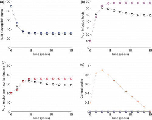
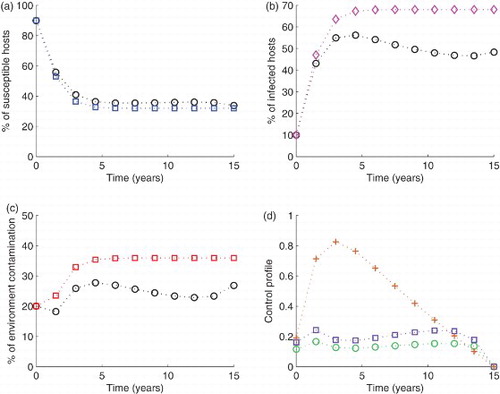
Figure 2. Simulation of the model with $u_1\ne 0,u_2=0,u_3=0.$ The blue circled line in (a), the pink diamond line in (b) and the red squared line in (c) show the model run in the absence of any control effort. In the same figures (i.e. (a), (b) and (c)), the circled black lines represent the variables run in the presence of control efforts described. In subfigure (d), the green circles are for control $u_1,$ purple square for $u_2$, and brown cross are for $u_3$. Other parameter values are given in Table 1 (Colour online).

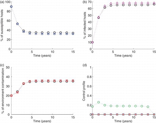
In Figures 2–4, each control is applied on its own, while setting others to zero. In comparison with no control, it is observed that with $u_1,$ the percentage increase in susceptibles is 5.05%, the infectives are reduced by 4.03% while neither increase nor reduction is observed in the proportion of contaminated environment. The highest level of control is 25.95% (Figure 2). For control $u_2,$ the percentage susceptible increase is 4.5%, I is reduced by 2.13% and C by 6.18%. However, it is important to note that this control reduced the level of contamination to 15.85%, which is 20.75% from the initial value (see Figure 3). The highest level of control is 40.47%. When control $u_3$ is used, the susceptibles are reduced by 5.80%, infectives by 10.26% and the environment by 7.93%, when the control applies at 90.6%. Note that among the three, this is the only control that reduced the number of susceptible population (Figure 4).

Figure 3. Simulation of the model with $u_1=0,u_2\ne 0,u_3=0.$ The blue circled line in (a), the pink diamond line in (b) and the red squared line in (c) show the model run in the absence of any control effort. In the same figures (i.e. (a), (b) and (c)), the circled black lines represent the variables run in the presence of control efforts described. In subfigure (d), the green circles are for control $u_1$, purple square for $u_2$, and brown cross are for $u_3$. Other parameter values are given in Table 1 (Colour online).

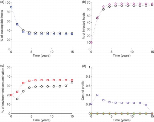
Figure 4. Simulation of the model with $u_1=0,u_2=0,u_3\ne 0.$ The blue circled line in (a), the pink diamond line in (b) and the red squared line in (c) show the model run in the absence of any control effort. In the same figures (i.e. (a), (b) and (c)), the circled black lines represent the variables run in the presence of control efforts described. In subfigure (d), the green circles are for control $u_1$, purple square for $u_2$, and brown cross are for $u_3$. Other parameter values are given in Table 1 (Colour online).

When the controls are applied in pairs while setting the third to zero, results indicate that for $u_1,u_2\ne 0,$ S increased by 38.40%, I reduced by 20.49% and C decreased from 35.95 to 26.01 (27.61%). With this combination, after 6 years, the level of contamination reduced from 20% to 2.44% (87.79% reduction, see Figure 5). With $u_1,u_3\ne 0,$ S decreased by 0.374%, I by 13.% and C by 9.21% (Figure 6). Finally $u_2,u_3\ne 0$ gave a 0.374 reduction in S, 13.46 in I and 18.12% in C (Figure 7).

Figure 5. Simulation of the model with $u_1\ne 0,u_2\ne 0,u_3=0.$ The blue circled line in (a), the pink diamond line in (b) and the red squared line in (c) show the model run in the absence of any control effort. In the same figures (i.e. (a), (b) and (c)), the circled black lines represent the variables run in the presence of control efforts described. In subfigure (d), the green circles are for control $u_1$, purple square for $u_2$, and brown cross are for $u_3$. Other parameter values are given in Table 1 (Colour online).

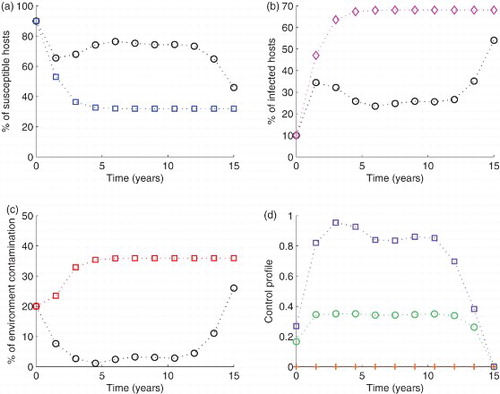
Figure 6. Simulation of the model with $u_1\ne 0,u_2=0,u_3\ne 0.$ The blue circled line in (a), the pink diamond line in (b) and the red squared line in (c) show the model run in the absence of any control effort. In the same figures (i.e. (a), (b) and (c)), the circled black lines represent the variables run in the presence of control efforts described. In subfigure (d), the green circles are for control $u_1$, purple square for $u_2$, and brown cross are for $u_3$. Other parameter values are given in Table 1 (Colour online).

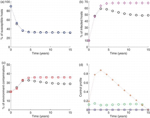
Figure 7. Simulation of the model with $u_1=0,u_2\ne 0,u_3\ne 0.$ The blue circled line in (a), the pink diamond line in (b) and the red squared line in (c) show the model run in the absence of any control effort. In the same figures (i.e. (a), (b) and (c)), the circled black lines represent the variables run in the presence of control efforts described. In subfigure (d), the green circles are for control $u_1$, purple square for $u_2$, and brown cross are for $u_3$. Other parameter values are given in Table 1 (Colour online).

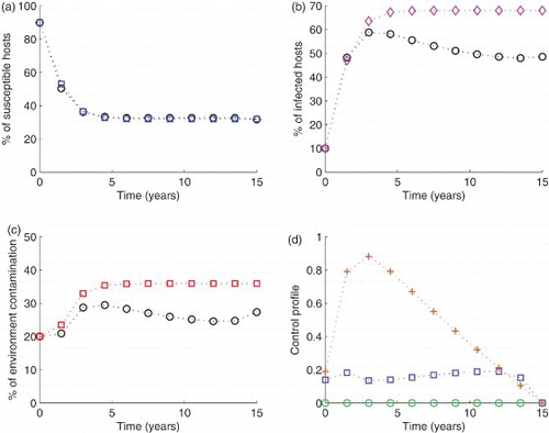
Figure 8. Simulation of the model with $u_1\ne 0,u_2\ne 0,u_3\ne 0.$ The blue circled line in (a), the pink diamond line in (b) and the red squared line in (c) show the model run in the absence of any control effort. In the same figures (i.e. (a), (b) and (c)), the circled black lines represent the variables run in the presence of control efforts described. In subfigure (d), the green circles are for control $u_1$, purple square for $u_2$, and brown cross are for $u_3$. Other parameter values are given in Table 1 (Colour online).

Finally, when all the controls are applied simultaneously, S increased by 5.27%, I reduced by 17.42 and C decreased by 22.85% (see Figure 8). This combination also reduced the level of contamination from 20% at $t=0$, to 18.22% at $t=1.5$. All these values are summarized in Table 3. With the above observations, the following conclusion is made:

Table 3. Table showing the highest and lowest values (in percentages), for each variable and the times at which they are achieved when different strategies for respective controls are applied.

		$u_1,u_2,u_3=0$	$u_1\ne 0$	$u_2\ne 0$	$u_3\ne 0$	$u_1,u_2\ne 0$	$u_1,u_3\ne 0$	$u_2,u_3\ne 0$	$u_1,u_2,u_3\ne 0$
S	Highest value	90	90	90	90	90	90	90	90
	Time	0	0	0	0	0	0	0	0
	Lowest value	32.08	33.70	33.41	30.22	76.48	31.96	31.96	33.77
	Time	6	15	15	15	6	9	9	15
I	Highest value	68.04	65.30	66.59	61.06	54.10	59.15	58.88	56.19
	Time	9	12	15	3	15	3	3	4.5
	Lowest value	10	10	10	10	10	10	10	10
	Time	0	0	0	0	0	0	0	0
C	Highest value	35.93	35.93	33.71	33.08	26.01	32.62	29.42	27.72
	Time	9	9	15	3	15	3	4.5	4.5
	Lowest value	20	20	15.85	20	2.442	20	20	18.22
	Time	0	0	1.5	0	6	0	0	1.5
$u_1$	At $t=0$	0	0.1683	0	0	0.2	0.1155	0	0.1155
	Highest value	–	0.2595	0	0	0.3442	0.1392	0	0.1660
	Time	0	1.5	–	–	1.5	1.5	–	1.5
$u_2$	At $t=0$	0	0	0.2	0	0.2686	0	0.1395	0.1613
	Highest value	0	0	0.4047	0	0.9542	0	0.1824	0.2419
	Time	–	–	1.5	–	3	–	1.5	1.5
$u_3$	At $t=0$	0	0	0	0.1871	0	0.1878	0.1890	0.1907
	Highest value	0	0	0	0.9060	0	0.8750	0.8823	0.8252
	Time	–	–	–	3	–	3	3	3

Corollary 3.1.

The best overall strategy for controlling brucellosis is a combination of $u_1$ and $u_2,$ which is preventing direct transmission while controlling the contamination of the environment, but it may not be the cheapest.

3.1. Discussion and conclusions

Table 3 summarizes the numerical results of our control problem in Figures 2– 8. The table gives the highest percentage values of the variables, together with the lowest values and the respective times they are attained. It is observed from the table that the highest percentage of non-infected susceptibles S (76.48%) is achieved when controls $u_1$ and $u_2$ are used in combination with each other. In turn, this gives the smallest percentage of non-removed infected subjects (54.10%), and the least per cent of contaminated environment, (2.442%). To achieve these results, control $u_1$ was applied at 34.42% (the highest value for this control in our profile) and control $u_2$ worked at 95.42%, which is also the highest nominal value among all controls. Thus, although effective, this profile may not be the cheapest. The second best control strategy is when all the three controls $u_1,u_2$ and $u_3$ are used in combination. This leaves only 33.77% of non-infected susceptibles, 56.19% non-removed infected and 18.22% proportion of contaminated environment. Looking at the values of the controls, it is further observed that to achieve this, $u_1$ works at 16.6%, $u_2$ at 24.19% and $u_3$ at 82.52%. Still, this may not provide the cheapest control method.

In conclusion, these results are obtained with the weight factors chosen for each control strategy. The true values of the weights are not well known and require extensive field work and data mining. The weights used here are intended only for theoretical purposes to investigate the effect of various control practices. The results can be improved by inclusion of the salvage term in the objective functional if the true weight values are known. In our study, however, inclusion of such a term would not have a significant impact on the overall conclusion of this optimal control problem. This has, however, availed to us with a future control problem.

Acknowledgements

The authors wish to thank the anonymous reviewers for the wonderful suggestions that made the manuscripts better.

Disclosure statement

No potential conflict of interest was reported by the authors.

References

- B. Aïnseba, C. Benosman, and P. Magal, A model for ovine brucellosis incorporating direct and indirect transmission, J. Biol. Dyn. 4 (2010), pp. 2–11. Available at http://www.math.u-bordeaux1.fr/~pmagal100p/papers/BBM-JBD09.pdf (Accessed 3 July 2012).
- A.H. Al-Talafhah, S.Q. Lafi, and Y. Al-Tarazi, Epidemiology of ovine brucellosis in awassi sheep in northern Jordan, Prev. Vet. Med. 60 (2003), pp. 297–306. doi: 10.1016/S0167-5877(03)00127-2
- V.S. Almeida and A.C. Louza, Simple mathematical modelling of brucellosis in portuguese dairy herds, Acta. Vet. Scand. Suppl. 84 (1988), pp. 477–479.
- S. Anita, V. Arnăutu, and V. Capasso, An Introduction to Optimal Control Problems in Life Sciences and Economics, Springer, New York, 2011.
- K. Blayney, Y. Cao, and H.D. Kwon, Optimal control of vector born diseases: treatment and prevention, Discrete Contin. Dyn. Syst. Ser. B (DCDS-B) 11 (2009), pp. 587–611. doi: 10.3934/dcdsb.2009.11.587
- B.M.D.C. Bronsvoort, B. Koterwas, F. Land, I.G. Handel, J. Tucker, K.L. Morgan, V.N. Tanya, T.H. Abdoel, and H.L. Smits, Comparison of a flow assay for brucellosis antibodies with the reference cELISA test in West African Bosindicus, PLoS ONE 4 (2009), p. e5221. doi: 10.1371/journal.pone.0005221
- R.S. Cantrell, C. Cosner, and W.F. Fagan, Brucellosis, boties, and brainworms: The impact of edge habitats on pathogen transmission and species extinction, J. Math. Biol. 42 (2001), pp. 95–119. doi: 10.1007/s002850000064
- N. Chitnis, J.M. Hyman, and J.M. Cushing, Determining important parameters in the spread of malaria through the sensitivity analysis of a mathematical model, Bull. Math. Biol. 70 (2008), pp. 1272–1296. doi: 10.1007/s11538-008-9299-0
- A. Dobson and M. Meagher, The population dynamics of brucellosis in the yellowstone national park, Ecology 77 (1996), pp. 1026–1036. doi: 10.2307/2265573
- P. van den Driessche and J. Watmough, Reproduction numbers and sub-threshold endemic equilibria for compartmental models of disease transmission, Math. Biosci. 180 (2002), pp. 29–48. doi: 10.1016/S0025-5564(02)00108-6
- W.H. Fleming and R.W. Rishel, Deterministic and Stochastic Optimal Control, Springer Verlag, New York, 1975.
- V.J.C. Fotheringham, Disinfection of livestock production premises, Rev. Sci. Tech. Off. Int. Epiz. 14 (1995), pp. 191–205.
- M. Galukande, S. Muwazi, and D.B. Mugisa, Aetiology of low back pain in Mulago Hospital, Uganda, Afr. Health Sci. 5 (2005), pp. 164–167.
- J.P. Ganiere, La brucellose animale, Ecoles Nationales Vérinaires Francaises, Merial (2004), pp. 1–47. Available at http://eve.vet-alfort.fr/pluginfile.php/32818/mod_resource/content/0/Poly%20Brucellose%2001-01-2014.pdf
- J. Gonzalez-Guzman and R. Naulin, Analysis of a model of bovine brucellosis using singular perturbations, J. Math. Biol. 33 (1994), pp. 211–234. doi: 10.1007/BF00160180
- R.A. Greenfield, D.A. Drevets, and L.J. Machado, Bacterial pathogens as biological weapons and agents of bioterrorism, Am. J. Med. Sci. 323 (2002), pp. 299–315. doi: 10.1097/00000441-200206000-00003
- M. Gwida, S. Al Dahouk, F. Melzer, U. Rösler, H. Neubauer, and H. Tomaso, Brucellosis? Regionally emerging zoonotic disease? Croat. Med. J. 51 (2010), pp. 289–295. doi: 10.3325/cmj.2010.51.289
- S.H. Hashemi, H. Keramat, M. Ranjbar, M. Mamani, A. Farzam, and S. Jamal-Omidi, Osteoarticular complications of brucellosis in hamedan, an endemic area in the west of iran, Int. J. Infect. Dis. 11 (2007), pp. 496–500. doi: 10.1016/j.ijid.2007.01.008
- R.H. Joshi, Optimal control of an HIV immunology model, Optim. Contr. Appl. Methods 2 (2002), pp. 199–213. doi: 10.1002/oca.710
- T. Kar and B. Ghosh, Sustainability and optimal control of an exploited prey predator system through provision of alternative food to predator, Biosystems (2012), pp. 220–232. doi: 10.1016/j.biosystems.2012.02.003
- J. Kunda, J. Fitzpatrick, R. Kazwala, N.P. French, G. Shirima, A. MacMillan, D. Kambarage, M. Bronsvoort, and S. Cleaveland, Health-seeking behaviour of human brucellosis cases in rural Tanzania, BMC Public Health 7 (2007), p. 315. doi: 10.1186/1471-2458-7-315
- S. Lenhart and J.T. Workman, Optimal Control Applied to Biological Models: Mathematical & Computational Biology, Chapman & Hall/CRC, Taylor & Francis Group, 2007. Available at https://www.crcpress.com/product/isbn/9781584886402
- B.G. Mantur and S.K. Amarnath, Brucellosis in India ? A review, J. Biosci. 33 (2008), pp. 539–547. doi: 10.1007/s12038-008-0072-1
- J.J. McDermott and S.M. Arimi, Brucellosis in sub-Saharan Africa: Epidemiology, control and impact, Vet. Microbiol. 90 (2002), pp. 111–134. doi: 10.1016/S0378-1135(02)00249-3
- J. McGiven, The improved specificity of bovine brucellosis testing in great britain, Res. Vet. Sci. 84 (2008), pp. 38–40. doi: 10.1016/j.rvsc.2007.03.003
- Medical Disability Advisor, Brucellosis. Available at http://www.mdguidelines.com/brucellosis (Accessed 13 March 2012).
- F. Melzer, S. Al Dahouk, H. Neubauer, and T.C. Mettenleiter, Increasing incidence in neighboring EU States. Is brucellosis about to become a travel medicine problem? MMW Fortschr Med 149 (2007), pp. 46–47.
- A. Minas, S. Minas, A. Stournara, and S. Tselepidis, The effects of Rev-1vaccination of sheep and goats on humans brucellosis in Greece, Prev. Vet. Med. 64 (2004), pp. 41–47. doi: 10.1016/j.prevetmed.2004.03.007
- J.B. Muma, N. Toft, J. Oloya, A. Lund, K. Nielsen, K. Samui, and E. Skjerve, Evaluation of three serological tests for brucellosis in naturally infected cattle using latent class analysis, Vet. Microbiol. 125 (2007), pp. 187–192. doi: 10.1016/j.vetmic.2007.05.012
- L.N. Mutanda, Selected laboratory tests in febrile patients in Kampala, Uganda, East Afr. Med. J. 75 (1998), pp. 68–72.
- L.S. Pontryagin, V.G. Boltyanskii, R.V. Gamkrelidze, and E.F. Mishechenko, The Mathematical Theory of Optimal Processes, Wiley, New York, 1962.
- F. Roth, J. Zinsstag, D. Orkhon, and G. Chimed-Ochir, Human health benefits from livestock vaccination for brucellosis, Bull. World Health Organ. 81 (2003), pp. 867–876.
- R. Rowthorn and F. Toxvaerd, The optimal control of infectious diseases via prevention and treatment. 2009. Available at: http://economics.yale.edu/sites/default/files/toxvaerd-130515.pdf (Accessed 27 July 2014).
- E.S. Swai and L. Schoonman, Human brucellosis: Seroprevalence and risk factors related to high risk occupational groups in Tanga Municipality, Tanzania, Zoonoses Public Health 56 (2009), pp. 183–187. doi: 10.1111/j.1863-2378.2008.01175.x
- WHO: Seven neglected endemic zoonoses – some basic facts. Zoonoses and Veterinary Public Health. Available at http://www.who.int/zoonoses/neglected_zoonotic_diseases/en/ (Accessed 3 July 2012).
- World Organisation for Animal Health (OIE), Chapter 2.4.3. Bovine brucellosis, in Manual of Diagnostic Tests and Vaccines for Terrestrial Animals, OIE, Paris, 2009. Available at http://www.oie.int/fileadmin/Home/eng/Health_standards/tahm/2.04.03_BOVINE_BRUCELL.pdf (Accessed 9 July 2013).
- E. Young, Brucella species, in Principles and Practice of Infectious Diseases, G.L. Mandell, J.E. Bennett, and R. Dolin, eds., Churchill-Livingstone, Philadelphia, 2000, pp. 2386–2393.