Modelling the biological invasion of Carcinus maenas (the European green crab)

ABSTRACT

This paper proposes a system of integro-difference equations to model the spread of Carcinus maenas, commonly called the European green crab, that causes severe damage to coastal ecosystems. A model with juvenile and adult classes is first studied. Here, standard theory of monotone operators for integro-difference equations can be applied and yields explicit formulas for the asymptotic spreading speeds of the juvenile and adult crabs. A second model including an infected class is considered by introducing a castrating parasite Sacculina carcini as a biological control agent. The dynamics are complicated and simulations reveal the occurrence of periodic solutions and stacked fronts. In this case, only conjectures can be made for the asymptotic spreading speeds because of the lack of mathematical theory for non-monotone operators. This paper also emphasizes the need for mathematical studies of non-monotone operators in heterogeneous environments and the existence of stacked front solutions in biological invasion models.

KEYWORDS:

• Asymptotic spreading speed
• biological invasions
• European green crab
• integro-difference equations
• stacked front solutions

AMS SUBJECT CLASSIFICATION:

• 39A60
• 92D25
• 92D40

1. Introduction

Biological invasions are considered to be one of the greatest threats to the integrity of most ecosystems on earth [31]. These invasions are seen in many kinds of species over a wide range of environments. Some recent examples include the Asian carp invading the Laurentian Great Lakes [35], zebra mussels invading freshwater lakes in North America [28], and the mountain pine beetle range expansion into Alberta, Canada [14]. This paper considers Carcinus maenas, commonly referred to as the European green crab, because it is native to the Atlantic, Baltic, and North Sea coasts of Europe from Mauritania to Norway [25].

C. maenas was first found in Cape Cod in 1817 [32] and discovered on the western coast of California in 1989 [13]. Since its arrival, the invasive green crab population has caused severe ecological and economic damage. In a field experiment on a mudflat in Pomquet Harbour, Nova Scotia C. maenas removed $80\mathrm{\%}$ of the softshell clam population [9]. Many other studies have also emphasized the detrimental effects of green crab predation on the fishing industry [6, 10, 16]. Colautti et al. estimated the potential economic impact of C. maenas on bivalve and crustacean fisheries and aquaculture in the Gulf of St. Lawrence to be approximately $\mathrm{\$}42\text{--}\mathrm{\$}109$ million [5]. The green crab invasion also affect the biodiversity of the ecosystem, for example, C. maenas have been reported to consume around $30\mathrm{\%}$ of the juvenile winter flounder population each year [36].

The use of mathematical models to study the spread of green crab to non-native ranges is not new. In 1996, Grosholz used a single-staged reaction diffusion model to study the spread of green crab [12]. The standard diffusion process can be easily modelled using a Gaussian dispersal kernel. In 2006, Byers and Pringle built a stage-structured model of benthic adult and platonic larvae stages [3]. In their model, the adults are sessile, while the larvae disperse through the water column. The main results show how variability in ocean currents can greatly influence the spread of a marine species, including upstream spread of green crab. In 2014, Kanary et al. used a stage-structured integro-difference equation model to study the effect of competition between two genotypes of green crab [18]. A primary result shown by the authors is that elimination of an established green crab population is essentially impossible by harvesting.

The motivation to study the spread of C. maenas is clear and one important question to address is whether a biological control agent could control the spread of this invasive species. Sacculina carcini, found in the green crabs native range, is a parasitic castrator of crabs that prevents the crab from moulting and reproducing [37]. When a female crab becomes infected with the parasite, the crab becomes unable to produce its own eggs and begins to treat the parasite's eggs as its own. After the parasite's eggs hatch, the newly born parasites can then spread through the water column to infect a host crab. In recent literature, the idea of using S. carcini as a biological control agent has been a popular topic [11, 37, 38]. In this paper, we extend the previous studies of green crab invasions by building and analysing a stage-structured integro-difference model that include the introduction of S. carcini as a biological control agent.

We choose to use a discrete-time mathematical model because the majority of the green crab reproduction is known to happen once a year during a short period triggered by the moulting of the female crab [19]. In order to understand the long-time behaviour of solutions to these types of models, we need the concept of asymptotic spreading speed. A simple way to explain this is via the following canonical example. Consider the recursion (1) $u_{t+1}\left(x\right)=Q\left[u_t\right]\left(x\right):={\int }_{-\mathrm{\infty }}^{\mathrm{\infty }}k(x-y)g\left(u_t\right(y\left)\right)\mathrm{d}y,$(1) where $k\left(x\right)$ is a probability density function, $g\in C^1[0,1]$ is a density-dependent growth function with the following properties: $g\left(0\right)=0,g\left(1\right)=1,g^{\mathrm{\prime }}\left(u\right)\ge 0,g^{\mathrm{\prime }}\left(0\right)>1,g\left(u\right)>u,$ and $g\left(u\right)\le g^{\mathrm{\prime }}\left(0\right)u$ in $[0,1]$. Then there exist two numbers, $c_{+}^{\ast }$ and $c_{-}^{\ast }$, such that if $u_0\in [0,1]$ is non-trivial and vanishes outside a finite interval, and we let $\{u_t,t\ge 0\}$ be the solutions of Equation (1(1) $u_{t+1}\left(x\right)=Q\left[u_t\right]\left(x\right):={\int }_{-\mathrm{\infty }}^{\mathrm{\infty }}k(x-y)g\left(u_t\right(y\left)\right)\mathrm{d}y,$(1) ), then $\underset{t\to \mathrm{\infty }}{lim}\underset{x\notin [-t{c}_1,t{c}_2]}{max}{u}_t\left(x\right)=0$ for any $c_2>c_{+}^{\ast }$ and $c_1>c_{-}^{\ast }$. Furthermore, $\underset{t\to \mathrm{\infty }}{lim}\underset{x\in [-t{c}_1,t{c}_2]}{min}{u}_t\left(x\right)=1$ for any $c_2<c_{+}^{\ast }$ and $c_1<c_{-}^{\ast }$. Thus, $c_{+}^{\ast }$ $\left(c_{-}^{\ast }\right)$ is commonly referred to as the asymptotic spreading speed of the operator Q in the positive (negative) x-direction.

Recursions of the form (1(1) $u_{t+1}\left(x\right)=Q\left[u_t\right]\left(x\right):={\int }_{-\mathrm{\infty }}^{\mathrm{\infty }}k(x-y)g\left(u_t\right(y\left)\right)\mathrm{d}y,$(1) ) have many applications in theoretical biology [20, 39, 40]. The above result about the asymptotic spreading speed of the operator Q has been generalized and an extension of it to systems is presented in Appendix 1. A very readable paper on this subject is the 1996 paper by Kot et al. [21].

The goal of this paper is to classify all potential behaviours for solutions of the model described by System (2(2) $\begin{array}{rl}{J}_{t+1}\left(x\right)& =s(1-m)(1-T_{\mathrm{p}}(x\left)\right)J_t\left(x\right)+{\int }_{-\mathrm{\infty }}^{\mathrm{\infty }}{k}_{\mathrm{c}}(x-y)f\left(A_t\right(y\left)\right)\mathrm{d}y,\\ A_{t+1}\left(x\right)& =sm(1-T_{\mathrm{p}}(x\left)\right)J_t\left(x\right)+s(1-T_{\mathrm{p}}(x\left)\right)A_t\left(x\right),\\ I_{t+1}\left(x\right)& =sm{T}_{\mathrm{p}}\left(x\right)J_t\left(x\right)+s{T}_{\mathrm{p}}\left(x\right)A_t\left(x\right)+s_{\mathrm{p}}{I}_t\left(x\right).\end{array}$(2) ) under different parameter relations and to explore the use of S. carcini as a biological control agent. It has been shown that there is much geographic variability in the green crab fecundity [38], survival [30], and dispersal [1]. Thus, we do not choose to fit the model to data, but provide a general framework that can be applied to a given region of interest.

The organization of this paper is as follows. In the next section, we present our integro-difference equation model to study the spread of the green crab. In Section 3, a special case consisting of only juvenile and adult populations is analysed. Then in Section 4 we analyse the model including the infection process by the castrating parasite. In this case, the dynamics are complicated and the behaviour of the solutions are captured primarily through simulations. We end the paper with some concluding remarks summarizing the main results and possible extensions to our work.

2. Mathematical model

We consider a stage-structured model of juvenile, adult, and infected crabs. The population density of juvenile, adult, and infected crabs at time t and location x are denoted by $J_t\left(x\right)$, $A_t\left(x\right)$, and $I_t\left(x\right)$, respectively. The following system of equations models the progression from year t to year $t+1$ of the green crabs: (2) $\begin{array}{rl}{J}_{t+1}\left(x\right)& =s(1-m)(1-T_{\mathrm{p}}(x\left)\right)J_t\left(x\right)+{\int }_{-\mathrm{\infty }}^{\mathrm{\infty }}{k}_{\mathrm{c}}(x-y)f\left(A_t\right(y\left)\right)\mathrm{d}y,\\ A_{t+1}\left(x\right)& =sm(1-T_{\mathrm{p}}(x\left)\right)J_t\left(x\right)+s(1-T_{\mathrm{p}}(x\left)\right)A_t\left(x\right),\\ I_{t+1}\left(x\right)& =sm{T}_{\mathrm{p}}\left(x\right)J_t\left(x\right)+s{T}_{\mathrm{p}}\left(x\right)A_t\left(x\right)+s_{\mathrm{p}}{I}_t\left(x\right).\end{array}$(2)

The progression of the juvenile class to the next generation can occur in two ways. First, some of the juvenile crabs survive to the next generation, do not mature, and do not get infected. This is represented by the first term on the right of the first equation of (2(2) $\begin{array}{rl}{J}_{t+1}\left(x\right)& =s(1-m)(1-T_{\mathrm{p}}(x\left)\right)J_t\left(x\right)+{\int }_{-\mathrm{\infty }}^{\mathrm{\infty }}{k}_{\mathrm{c}}(x-y)f\left(A_t\right(y\left)\right)\mathrm{d}y,\\ A_{t+1}\left(x\right)& =sm(1-T_{\mathrm{p}}(x\left)\right)J_t\left(x\right)+s(1-T_{\mathrm{p}}(x\left)\right)A_t\left(x\right),\\ I_{t+1}\left(x\right)& =sm{T}_{\mathrm{p}}\left(x\right)J_t\left(x\right)+s{T}_{\mathrm{p}}\left(x\right)A_t\left(x\right)+s_{\mathrm{p}}{I}_t\left(x\right).\end{array}$(2) ), where s is the survival probability, m is the probability of maturation, and $T_{\mathrm{p}}\left(x\right)$ is the probability of transmission of the parasite. The second way is when the adult crabs at location y produce larvae at the rate according to the fecundity function $f\left(A_t\right(y\left)\right)$, and the larvae then disperse from location y to x according to the dispersal kernel $k_{\mathrm{c}}(x-y)$. Since we have to include dispersal from all locations y to x, we integrate the product of the dispersal kernel with the fecundity function over $\mathbb{R}$. After the dispersal, the larvae mature to become juveniles in the next generation. This process is represented by the last term of the first equation of (2(2) $\begin{array}{rl}{J}_{t+1}\left(x\right)& =s(1-m)(1-T_{\mathrm{p}}(x\left)\right)J_t\left(x\right)+{\int }_{-\mathrm{\infty }}^{\mathrm{\infty }}{k}_{\mathrm{c}}(x-y)f\left(A_t\right(y\left)\right)\mathrm{d}y,\\ A_{t+1}\left(x\right)& =sm(1-T_{\mathrm{p}}(x\left)\right)J_t\left(x\right)+s(1-T_{\mathrm{p}}(x\left)\right)A_t\left(x\right),\\ I_{t+1}\left(x\right)& =sm{T}_{\mathrm{p}}\left(x\right)J_t\left(x\right)+s{T}_{\mathrm{p}}\left(x\right)A_t\left(x\right)+s_{\mathrm{p}}{I}_t\left(x\right).\end{array}$(2) ). We shall return to discuss f, $T_{\mathrm{p}}$, and $k_{\mathrm{c}}$ later in this section.

The progression to the next generation of the adult class can occur in two ways: juveniles can mature into the adult class if they survive, mature, and do not get infected, or adult crabs can remain adults if they survive but do not get infected. This is described by the second equation of (2(2) $\begin{array}{rl}{J}_{t+1}\left(x\right)& =s(1-m)(1-T_{\mathrm{p}}(x\left)\right)J_t\left(x\right)+{\int }_{-\mathrm{\infty }}^{\mathrm{\infty }}{k}_{\mathrm{c}}(x-y)f\left(A_t\right(y\left)\right)\mathrm{d}y,\\ A_{t+1}\left(x\right)& =sm(1-T_{\mathrm{p}}(x\left)\right)J_t\left(x\right)+s(1-T_{\mathrm{p}}(x\left)\right)A_t\left(x\right),\\ I_{t+1}\left(x\right)& =sm{T}_{\mathrm{p}}\left(x\right)J_t\left(x\right)+s{T}_{\mathrm{p}}\left(x\right)A_t\left(x\right)+s_{\mathrm{p}}{I}_t\left(x\right).\end{array}$(2) ).

The progression of the infected class can occur in three ways. First, juveniles can survive, mature into adults, and become infected. Second, adult crabs can survive and be infected. Finally, infected crabs can survive to the next generation where the survival probability of infected crabs is denoted by $s_{\mathrm{p}}$. These three processes are summarized by the third equation in (2(2) $\begin{array}{rl}{J}_{t+1}\left(x\right)& =s(1-m)(1-T_{\mathrm{p}}(x\left)\right)J_t\left(x\right)+{\int }_{-\mathrm{\infty }}^{\mathrm{\infty }}{k}_{\mathrm{c}}(x-y)f\left(A_t\right(y\left)\right)\mathrm{d}y,\\ A_{t+1}\left(x\right)& =sm(1-T_{\mathrm{p}}(x\left)\right)J_t\left(x\right)+s(1-T_{\mathrm{p}}(x\left)\right)A_t\left(x\right),\\ I_{t+1}\left(x\right)& =sm{T}_{\mathrm{p}}\left(x\right)J_t\left(x\right)+s{T}_{\mathrm{p}}\left(x\right)A_t\left(x\right)+s_{\mathrm{p}}{I}_t\left(x\right).\end{array}$(2) ).

We now return to discuss the fecundity function f. Fecundity is defined as the physiological maximum potential reproductive output of an individual [2]. For the green crab, we assume that f has the following functional form: (3) $f\left(A_t\right(y\left)\right):=f_0{\mathrm{e}}^{-\gamma A_t\left(y\right)}{A}_t\left(y\right),$(3) which is commonly called a Ricker function. The use of a Ricker function is advantageous if there is overcompensation in a population from density dependence. One common way that overcompensation is seen in marine organisms is through cannibalism of their own larvae. The European green crab is known to consume its own larvae when resources are scarce [27]. In a 2014 paper, Miller and Morgan showed that recently ovigerous female shore crabs consumed 25–30% of their own larvae, whereas non-ovigerous crabs consumed 90% of the larvae [26]. The authors also found that there is a positive relationship between the amount of time that the crab was starved and the increase in cannibalism of larvae. It is therefore more appropriate to use a Ricker function than a Beverton–Holt function for fecundity.

One important feature of the model is that the parasite populations are not modelled directly; only the stage-structured crab populations are directly modelled. The parasite interactions are incorporated into the infected population. The infected crabs do not infect the juvenile and adult class by direct contact. Transmission of the parasite occurs from an infected crab that releases σ parasites into the water, where σ is the average number of parasites produced per infected female. Then the parasites at location y disperse to location x according to the probability density function $k_{\mathrm{p}}(x-y)$, and attempt to find a host to infect. For brevity, we define the underlying dispersal of the parasite released from a host by $L_{\mathrm{p}}\left(x\right)$. In the model, we assume that $T_{\mathrm{p}}\left(x\right)\in [0,1]$ and is an increasing function of $L_{\mathrm{p}}\left(x\right)$. Thus, $T_{\mathrm{p}}\left(x\right)$ and $L_{\mathrm{p}}\left(x\right)$ are defined by (4) $T_{\mathrm{p}}\left(x\right):=\frac{L_{\mathrm{p}}\left(x\right)}{\rho +L_{\mathrm{p}}\left(x\right)}$(4) (5) $\mathrm{and}{L}_{\mathrm{p}}\left(x\right):={\int }_{-\mathrm{\infty }}^{\mathrm{\infty }}{k}_{\mathrm{p}}(x-y)\sigma I_t\left(y\right)dy,$(5) where ρ is a positive scaling constant.

In System (2(2) $\begin{array}{rl}{J}_{t+1}\left(x\right)& =s(1-m)(1-T_{\mathrm{p}}(x\left)\right)J_t\left(x\right)+{\int }_{-\mathrm{\infty }}^{\mathrm{\infty }}{k}_{\mathrm{c}}(x-y)f\left(A_t\right(y\left)\right)\mathrm{d}y,\\ A_{t+1}\left(x\right)& =sm(1-T_{\mathrm{p}}(x\left)\right)J_t\left(x\right)+s(1-T_{\mathrm{p}}(x\left)\right)A_t\left(x\right),\\ I_{t+1}\left(x\right)& =sm{T}_{\mathrm{p}}\left(x\right)J_t\left(x\right)+s{T}_{\mathrm{p}}\left(x\right)A_t\left(x\right)+s_{\mathrm{p}}{I}_t\left(x\right).\end{array}$(2) ) and Equation (5(5) $\mathrm{and}{L}_{\mathrm{p}}\left(x\right):={\int }_{-\mathrm{\infty }}^{\mathrm{\infty }}{k}_{\mathrm{p}}(x-y)\sigma I_t\left(y\right)dy,$(5) ), $k_{\mathrm{c}}$ and $k_{\mathrm{p}}$ are probability density functions, which model the dispersion of crab larvae and parasites, respectively. They are assumed to be asymmetric Laplace distributions instead of the traditional Gaussian distribution because the crab larvae and parasites are known to be transported in the water due to the ocean current with a constant settling rate. The dispersal kernels have the form (6) $\begin{array}{r}{k}_{\mathrm{c}}\left(x\right):=\frac{a_{{\mathrm{c}}_1}{a}_{{\mathrm{c}}_2}}{a_{{\mathrm{c}}_2}-a_{{\mathrm{c}}_1}}\left\{\begin{array}{l}{\mathrm{e}}^{a_{{\mathrm{c}}_1}x}x\le 0,,\\ {\mathrm{e}}^{a{}_{c_2}{}_{{\mathrm{c}}_2}x}& x>0,\end{array}\right.\end{array}$(6) (7) $\begin{array}{r}\mathrm{and}{k}_{\mathrm{p}}\left(x\right):=\frac{a_{{\mathrm{p}}_1}{a}_{{\mathrm{p}}_2}}{a_{{\mathrm{p}}_2}-a_{{\mathrm{p}}_1}}\left\{\begin{array}{ll}{\mathrm{e}}^{a_{{\mathrm{p}}_1}x}& x\le 0,\\ {\mathrm{e}}^{a_{{\mathrm{p}}_2}x}& x>0,\end{array}\right.\end{array}$(7) where (8) $a_{{\mathrm{c}}_1,{\mathrm{c}}_2}:=\frac{v}{2D}\pm \sqrt{{\left(\frac{v}{2D}\right)}^2+\frac{{\alpha }_{\mathrm{c}}}{D}},$(8) (9) $\mathrm{and}{a}_{{\mathrm{p}}_1,{\mathrm{p}}_2}:=\frac{v}{2D}\pm \sqrt{{\left(\frac{v}{2D}\right)}^2+\frac{{\alpha }_{\mathrm{p}}}{D}}.$(9) In Equations (8(8) $a_{{\mathrm{c}}_1,{\mathrm{c}}_2}:=\frac{v}{2D}\pm \sqrt{{\left(\frac{v}{2D}\right)}^2+\frac{{\alpha }_{\mathrm{c}}}{D}},$(8) ) and (9(9) $\mathrm{and}{a}_{{\mathrm{p}}_1,{\mathrm{p}}_2}:=\frac{v}{2D}\pm \sqrt{{\left(\frac{v}{2D}\right)}^2+\frac{{\alpha }_{\mathrm{p}}}{D}}.$(9) ), v is the advection speed of the current, D is the diffusion coefficient, and ${\alpha }_{\mathrm{c}}$ and ${\alpha }_{\mathrm{p}}$ are the settling rates for crab larvae and parasites, respectively. The formulas for $a_{{\mathrm{c}}_1,{\mathrm{c}}_2}$ and $a_{{\mathrm{p}}_1,{\mathrm{p}}_2}$ are commonly used for modelling the dispersion of an organism that diffuses in an advective current with a constant dropout probability [24]. Note that the advection speed and the diffusion coefficient are the same for the crab larvae and parasite because they disperse in the same water column. Here, the current is assumed to flow in the positive x-direction. From Equations (8(8) $a_{{\mathrm{c}}_1,{\mathrm{c}}_2}:=\frac{v}{2D}\pm \sqrt{{\left(\frac{v}{2D}\right)}^2+\frac{{\alpha }_{\mathrm{c}}}{D}},$(8) ) and (9(9) $\mathrm{and}{a}_{{\mathrm{p}}_1,{\mathrm{p}}_2}:=\frac{v}{2D}\pm \sqrt{{\left(\frac{v}{2D}\right)}^2+\frac{{\alpha }_{\mathrm{p}}}{D}}.$(9) ), $a_{{\mathrm{c}}_2},a_{{\mathrm{p}}_2}<0<a_{{\mathrm{c}}_1},a_{{\mathrm{p}}_1}$ and $a_{{\mathrm{c}}_1}+a_{{\mathrm{c}}_2}=a_{{\mathrm{p}}_1}+a_{{\mathrm{p}}_2}=v/D>0$.

Throughout this paper, we assume that $f_0>1,s,s_{\mathrm{p}}\in (0,1),m\in (0,1]$ and $\gamma >0$. The values $s,s_{\mathrm{p}},m=0$ are not considered because these cases make drastic yet uninteresting simplifications to the model. When $s=0$ $(s_{\mathrm{p}}=0)$, biologically this means that crabs not infected (infected) by the parasites cannot survive. When $m=0$, the biological meaning is that a juvenile crab never mature into an adult crab. We now present the mathematical analysis of the model.

3. The juvenile–adult model

We first consider the case when there are no infected crabs in the population. This is a special case of System (2(2) $\begin{array}{rl}{J}_{t+1}\left(x\right)& =s(1-m)(1-T_{\mathrm{p}}(x\left)\right)J_t\left(x\right)+{\int }_{-\mathrm{\infty }}^{\mathrm{\infty }}{k}_{\mathrm{c}}(x-y)f\left(A_t\right(y\left)\right)\mathrm{d}y,\\ A_{t+1}\left(x\right)& =sm(1-T_{\mathrm{p}}(x\left)\right)J_t\left(x\right)+s(1-T_{\mathrm{p}}(x\left)\right)A_t\left(x\right),\\ I_{t+1}\left(x\right)& =sm{T}_{\mathrm{p}}\left(x\right)J_t\left(x\right)+s{T}_{\mathrm{p}}\left(x\right)A_t\left(x\right)+s_{\mathrm{p}}{I}_t\left(x\right).\end{array}$(2) ) with $T_{\mathrm{p}}\left(x\right)=0$. We use this model to study how the invasive crabs spread in the absence of the parasite. The juvenile–adult (JA) model is (10) $\begin{array}{rl}{J}_{t+1}\left(x\right)& =s(1-m)J_t\left(x\right)+{\int }_{-\mathrm{\infty }}^{\mathrm{\infty }}{k}_{\mathrm{c}}(x-y)f\left(A_t\right(y\left)\right)\mathrm{d}y,\\ A_{t+1}\left(x\right)& =sm{J}_t\left(x\right)+s{A}_t\left(x\right),\end{array}$(10) where f and $k_{\mathrm{c}}$ are defined by Equations (3(3) $f\left(A_t\right(y\left)\right):=f_0{\mathrm{e}}^{-\gamma A_t\left(y\right)}{A}_t\left(y\right),$(3) ) and (6(6) $\begin{array}{r}{k}_{\mathrm{c}}\left(x\right):=\frac{a_{{\mathrm{c}}_1}{a}_{{\mathrm{c}}_2}}{a_{{\mathrm{c}}_2}-a_{{\mathrm{c}}_1}}\left\{\begin{array}{l}{\mathrm{e}}^{a_{{\mathrm{c}}_1}x}x\le 0,,\\ {\mathrm{e}}^{a{}_{c_2}{}_{{\mathrm{c}}_2}x}& x>0,\end{array}\right.\end{array}$(6) ), respectively. Since $f^{\mathrm{\prime }}\left(A\right)=f_0(1-\gamma A){\mathrm{e}}^{-\gamma A}$, we have $f\left(A\right)\le f^{\mathrm{\prime }}\left(0\right)A$ for $A\ge 0$. Furthermore, if $0\le A\le 1/\gamma$, the right side of System (10(11) $\begin{array}{rl}{J}_{t+1}& =s(1-m)J_t+f_0{\mathrm{e}}^{-\gamma A_t}{A}_t,\\ A_{t+1}& =sm{J}_t+s{A}_t.\end{array}$(11) ) is a monotone operator.

3.1. Analysis of the steady states

Consider System (10(11) $\begin{array}{rl}{J}_{t+1}& =s(1-m)J_t+f_0{\mathrm{e}}^{-\gamma A_t}{A}_t,\\ A_{t+1}& =sm{J}_t+s{A}_t.\end{array}$(11) ) without dispersion: (11) $\begin{array}{rl}{J}_{t+1}& =s(1-m)J_t+f_0{\mathrm{e}}^{-\gamma A_t}{A}_t,\\ A_{t+1}& =sm{J}_t+s{A}_t.\end{array}$(11) In what follows, stability means linear stability. A steady state solution is stable if the eigenvalues of the Jacobian matrix evaluated at the steady state lie inside the unit circle in the complex plane. There are only two steady states : $(J_0,A_0)=\mathbf{\text{0}}$ the extirpation steady state and $(J^{\ast },A^{\ast })$ the non-trivial steady state, where (12) $J^{\ast }=\frac{1-s}{sm}{A}^{\ast }$(12) (13) $\mathrm{and}{A}^{\ast }=-\frac{1}{\gamma }\ln \left[\frac{(1-s)(1-s(1-m\left)\right)}{f_{0}sm}\right].$(13) Note that $A^{\ast }>0$ if and only if (14) $f_0>\frac{(1-s)(1-s(1-m\left)\right)}{sm}.$(14) We assume that $f_{0}sm\ne (1-s)(1-s(1-m\left)\right)$ so that $(J^{\ast },A^{\ast })\ne \mathbf{\text{0}}$.

Proposition 3.1.

Let $A^{\ast }<1/\gamma$. Then the stability of the steady states can be classified as follows:

1. If $(J^{\ast },A^{\ast })$ exists in the positive quadrant, then it is stable and $(J_0,A_0)$ is unstable.

2. If $(J^{\ast },A^{\ast })$ does not exist in the positive quadrant, then $(J_0,A_0)$ is stable.

Proof.

We divide the proof into the two cases.

1. The Jacobian matrix evaluated at the steady state $(J^{\ast },A^{\ast })$ is (15) $M^{\ast }:=\left[\begin{array}{cc}s(1-m)& (1-\gamma A^{\ast })f_0{\mathrm{e}}^{-\gamma A^{\ast }}\\ sm& s\end{array}\right].$(15) The characteristic polynomial of $M^{\ast }$ has the form ${\lambda }^2-\beta \lambda +\alpha =0$, where $\beta =s(2-m)\ge 0$ and $1+\alpha =1+s^2(1-m)-(1-\gamma A^{\ast })sm{f}_0{\mathrm{e}}^{-\gamma A^{\ast }}<2$. Then $(J^{\ast },A^{\ast })$ is stable if and only if $|\lambda |<1$. From [7], $|\lambda |<1$ if and only if $|\beta |<1+\alpha <2$. Also, (16) $\beta <1+\alpha ⟺-1<-(1-\gamma A^{\ast }).$(16) The last inequality is valid since $A^{\ast }>0$. Therefore, if $(J^{\ast },A^{\ast })$ exists it is stable.

2. The Jacobian matrix at the origin is (17) $M_0:=\left[\begin{array}{cc}s(1-m)& f_0\\ sm& s\end{array}\right].$(17) The characteristic equation is $P\left(\lambda \right)\equiv {\lambda }^2-s(2-m)\lambda +s^2(1-m)-sm{f}_0=0$. The condition $\beta <1+\alpha$ is equivalent to (18) $f_0<\frac{(1-s)(1-s(1-m\left)\right)}{sm}.$(18) However, this is the opposite of condition (14(14) $f_0>\frac{(1-s)(1-s(1-m\left)\right)}{sm}.$(14) ). Therefore, if $(J^{\ast },A^{\ast })$ does lie in the positive quadrant, the origin is stable. The proof of the proposition is complete.

3.2. Determining the asymptotic spreading speed

We now consider the model with dispersion. Let ${\mathbf{\text{u}}}_t=[J_t,A_t{]}^{\mathrm{T}}$, and let $\mathbf{\text{Q}}\left[{\mathbf{\text{u}}}_t\right]$ denote the operator on the right side of System (10(11) $\begin{array}{rl}{J}_{t+1}& =s(1-m)J_t+f_0{\mathrm{e}}^{-\gamma A_t}{A}_t,\\ A_{t+1}& =sm{J}_t+s{A}_t.\end{array}$(11) ). Let $\mathit{\beta }=(J^{\ast },A^{\ast })$. The linearization of $\mathbf{\text{Q}}$ at the origin is (19) $\mathbf{\text{M}}\left[\mathbf{\text{u}}\right]\left(x\right):={\int }_{-\mathrm{\infty }}^{\mathrm{\infty }}\left[K\right(x-y)\circ L]\mathbf{\text{u}}\left(y\right)\mathrm{d}y,$(19) where (20) $L=\left[\begin{array}{cc}s(1-m)& f_0\\ sm& s\end{array}\right],K\left(x\right)=\left[\begin{array}{cc}{\delta }_0& k_{\mathrm{c}}\left(x\right)\\ {\delta }_0& {\delta }_0\end{array}\right],$(20) $\circ$ denotes the Hadamard product, $k_{\mathrm{c}}$ is defined by Equation (6(6) $\begin{array}{r}{k}_{\mathrm{c}}\left(x\right):=\frac{a_{{\mathrm{c}}_1}{a}_{{\mathrm{c}}_2}}{a_{{\mathrm{c}}_2}-a_{{\mathrm{c}}_1}}\left\{\begin{array}{l}{\mathrm{e}}^{a_{{\mathrm{c}}_1}x}x\le 0,,\\ {\mathrm{e}}^{a{}_{c_2}{}_{{\mathrm{c}}_2}x}& x>0,\end{array}\right.\end{array}$(6) ), and ${\delta }_0$ is the Dirac-delta function concentrated at the origin. The following result follows from Proposition A.1 in Appendix 1.

Proposition 3.2.

Let the hypotheses of Proposition 3.1 and Equation (14(14) $f_0>\frac{(1-s)(1-s(1-m\left)\right)}{sm}.$(14) ) hold. Then the asymptotic spreading speeds of the operator $\mathbf{Q}$ in the positive and negative x-directions are given by (21) $c_{+}^{\ast }=\underset{0<z<-a_{{\mathrm{c}}_2}}{min}\left[\frac{1}{z}\ln \left({\rho }_{+}\right(z\left)\right)\right]$(21) and (22) $c_{-}^{\ast }=\underset{0<z<a_{{\mathrm{c}}_1}}{min}\left[\frac{1}{z}\ln \left({\rho }_{-}\right(z\left)\right)\right],$(22) respectively, where (23) ${\rho }_{+}\left(z\right)=s\left(1-\frac{1}{2}m\right)+\frac{1}{2}\sqrt{(sm{)}^2+\frac{4f_{0}sm{a}_{{\mathrm{c}}_1}{a}_{{\mathrm{c}}_2}}{(z+a_{{\mathrm{c}}_1})(z+a_{{\mathrm{c}}_2})}},$(23) (24) ${\rho }_{-}\left(z\right)=s\left(1-\frac{1}{2}m\right)+\frac{1}{2}\sqrt{(sm{)}^2+\frac{4f_{0}sm{a}_{{\mathrm{c}}_1}{a}_{{\mathrm{c}}_2}}{(z-a_{{\mathrm{c}}_1})(z-a_{{\mathrm{c}}_2})}}.$(24)

Proof.

Recall that $a_{{\mathrm{c}}_2}<0<a_{{\mathrm{c}}_1}$. For the asymmetric Laplace distribution, the moment generating function for the crab dispersion kernel is (25) $m_{+}\left(z\right)={\int }_{-\mathrm{\infty }}^{\mathrm{\infty }}{k}_{\mathrm{c}}\left(x\right){\mathrm{e}}^{zx}\mathrm{d}x=\frac{a_{{\mathrm{c}}_1}{a}_{{\mathrm{c}}_2}}{(z+a_{{\mathrm{c}}_1})(z+a_{{\mathrm{c}}_2})}$(25) for $-a_{{\mathrm{c}}_1}<z<-a_{{\mathrm{c}}_2}$. Similarly, (26) $m_{-}\left(z\right)={\int }_{-\mathrm{\infty }}^{\mathrm{\infty }}{k}_{\mathrm{c}}\left(x\right){\mathrm{e}}^{-zx}\mathrm{d}x=\frac{a_{{\mathrm{c}}_1}{a}_{{\mathrm{c}}_2}}{(z-a_{{\mathrm{c}}_1})(z-a_{{\mathrm{c}}_2})}$(26) for $a_{{\mathrm{c}}_2}<z<a_{{\mathrm{c}}_1}$. From Proposition A.1, the asymptotic spreading speeds for the operator $\mathbf{Q}$ in the positive and negative x-directions are given by (27) $c_{+}^{\ast }=\underset{0<z<-a_{{\mathrm{c}}_2}}{min}\left[\frac{1}{z}\ln {\rho }_{+}\left(z\right)\right]\mathrm{and}{c}_{-}^{\ast }=\underset{0<z<+a_{{\mathrm{c}}_1}}{min}\left[\frac{1}{z}\ln {\rho }_{-}\left(z\right)\right],$(27) respectively, where ${\rho }_{\pm }\left(z\right)$ are the largest eigenvalues of (28) $B_{\pm }\left(z\right)=\left[\begin{array}{cc}s(1-m)& \frac{f_0{a}_{{\mathrm{c}}_1}{a}_{{\mathrm{c}}_2}}{(z\pm a_{{\mathrm{c}}_1})(z\pm a_{{\mathrm{c}}_2})}\\ sm& s\end{array}\right].$(28) It is easy to verify that (29) ${\rho }_{\pm }\left(z\right)=s\left(1-\frac{1}{2}m\right)+\frac{1}{2}\sqrt{(sm{)}^2+\frac{4f_{0}sm{a}_{{\mathrm{c}}_1}{a}_{{\mathrm{c}}_2}}{(z\pm a_{{\mathrm{c}}_1})(z\pm a_{{\mathrm{c}}_2})}}.$(29) The proof of the proposition is complete.

Remark 1.

We now show that $c_{+}^{\ast }>0$. The characteristic equation of $B_{+}\left(z\right)$ is $P_{+}\left(\lambda \right)=\left(s\right(1-m)-\lambda )(s-\lambda )-f_{0}sm{a}_{{\mathrm{c}}_1}{a}_{{\mathrm{c}}_2}/\left(\right(z+a_{{\mathrm{c}}_1}\left)\right(z+a_{{\mathrm{c}}_2}\left)\right)$. The condition ${\rho }_{+}\left(z\right)>1$ is the same as $P_{+}\left(1\right)<0$, or (30) $z^2+(a_{{\mathrm{c}}_1}+a_{{\mathrm{c}}_2})z+a_{{\mathrm{c}}_1}{a}_{{\mathrm{c}}_2}-\frac{f_{0}sm{a}_{{\mathrm{c}}_1}{a}_{{\mathrm{c}}_2}}{(1-s)(1-s(1-m\left)\right)}>0,$(30) for $0<z<-a_{{\mathrm{c}}_2}$. Since $a_{{\mathrm{c}}_1}+a_{{\mathrm{c}}_2}>0$, the minimum of this quadratic polynomial occurs at $z=0$. Thus, $c_{+}^{\ast }>0$ if (31) $f_0>\frac{(1-s)(1-s(1-m\left)\right)}{sm}.$(31) Note that Equation (31(30) $z^2+(a_{{\mathrm{c}}_1}+a_{{\mathrm{c}}_2})z+a_{{\mathrm{c}}_1}{a}_{{\mathrm{c}}_2}-\frac{f_{0}sm{a}_{{\mathrm{c}}_1}{a}_{{\mathrm{c}}_2}}{(1-s)(1-s(1-m\left)\right)}>0,$(30) ) is the same as condition (14(14) $f_0>\frac{(1-s)(1-s(1-m\left)\right)}{sm}.$(14) ), the requirement for $(J^{\ast },A^{\ast })$ to exist in the positive quadrant and to be stable. Therefore, we can conclude that $c_{+}^{\ast }$ is always positive. Next, we find the condition for $c_{-}^{\ast }>0$. The characteristic equation of $B_{-}\left(z\right)$ is $P_{-}\left(\lambda \right)=\left(s\right(1-m)-\lambda )(s-\lambda )-f_{0}sm{a}_{{\mathrm{c}}_1}{a}_{{\mathrm{c}}_2}/\left(\right(z-a_{{\mathrm{c}}_1}\left)\right(z-a_{{\mathrm{c}}_2}\left)\right)$. The condition $P_{-}\left(1\right)<0$ is the same as (32) $z^2-(a_{{\mathrm{c}}_1}+a_{{\mathrm{c}}_2})z+a_{{\mathrm{c}}_1}{a}_{{\mathrm{c}}_2}-\frac{f_{0}sm{a}_{{\mathrm{c}}_1}{a}_{{\mathrm{c}}_2}}{(1-s)(1-s(1-m\left)\right)}>0,$(32) for $0<z<a_{{\mathrm{c}}_1}$. The minimum occurs at $z=(a_{{\mathrm{c}}_1}+a_{{\mathrm{c}}_2})/2$. The condition $c_{-}^{\ast }>0$ is guaranteed by the inequality (33) $-\frac{v^2}{4D^2}+\frac{{\alpha }_{\mathrm{c}}}{D}\left(\frac{f_{0}sm}{(1-s)(1-s(1-m\left)\right)}-1\right)>0.$(33) Thus, $c_{-}^{\ast }$ can become negative if the current is too strong. From the definition of $k_{\mathrm{c}}\left(x\right)$ it is clear that $c_{-}^{\ast }<c_{+}^{\ast }$.

4. The juvenile–adult–infected model

In this section, we consider model (2(2) $\begin{array}{rl}{J}_{t+1}\left(x\right)& =s(1-m)(1-T_{\mathrm{p}}(x\left)\right)J_t\left(x\right)+{\int }_{-\mathrm{\infty }}^{\mathrm{\infty }}{k}_{\mathrm{c}}(x-y)f\left(A_t\right(y\left)\right)\mathrm{d}y,\\ A_{t+1}\left(x\right)& =sm(1-T_{\mathrm{p}}(x\left)\right)J_t\left(x\right)+s(1-T_{\mathrm{p}}(x\left)\right)A_t\left(x\right),\\ I_{t+1}\left(x\right)& =sm{T}_{\mathrm{p}}\left(x\right)J_t\left(x\right)+s{T}_{\mathrm{p}}\left(x\right)A_t\left(x\right)+s_{\mathrm{p}}{I}_t\left(x\right).\end{array}$(2) ). For simplicity, we assume that $s_{\mathrm{p}}=s$ and $m=1$. It is reasonable to assume that $m=1$ if the amount of time it takes for a juvenile crab to mature is relatively short compared to the time scale of the model. We also scale our model by multiplying each stage by $\sigma /\rho$ and redefining $\sigma J_t/\rho ,\sigma A_t/\rho ,\sigma I_t/\rho$ as the new $J_t,A_t,I_t$, respectively. We also let $\gamma \rho /\sigma$ be the new γ. The non-dimensionalized model is given by the following system of integro-difference equations: (34) $\begin{array}{rl}{J}_{t+1}\left(x\right)& ={\int }_{-\mathrm{\infty }}^{\mathrm{\infty }}{k}_{\mathrm{c}}(x-y)f\left(A_t\right(y\left)\right)\mathrm{d}y,\\ A_{t+1}\left(x\right)& =s\left(J_t\right(x)+A_t(x\left)\right)(1-T_{\mathrm{p}}(x\left)\right),\\ I_{t+1}\left(x\right)& =s\left(J_t\right(x)+A_t(x\left)\right)T_{\mathrm{p}}\left(x\right)+s{I}_t\left(x\right),\end{array}$(34) where f defined by Equation (3(3) $f\left(A_t\right(y\left)\right):=f_0{\mathrm{e}}^{-\gamma A_t\left(y\right)}{A}_t\left(y\right),$(3) ) denotes juveniles produced in the next generation and $k_{\mathrm{c}}$ defined by Equations (6(6) $\begin{array}{r}{k}_{\mathrm{c}}\left(x\right):=\frac{a_{{\mathrm{c}}_1}{a}_{{\mathrm{c}}_2}}{a_{{\mathrm{c}}_2}-a_{{\mathrm{c}}_1}}\left\{\begin{array}{l}{\mathrm{e}}^{a_{{\mathrm{c}}_1}x}x\le 0,,\\ {\mathrm{e}}^{a{}_{c_2}{}_{{\mathrm{c}}_2}x}& x>0,\end{array}\right.\end{array}$(6) ) and (8(8) $a_{{\mathrm{c}}_1,{\mathrm{c}}_2}:=\frac{v}{2D}\pm \sqrt{{\left(\frac{v}{2D}\right)}^2+\frac{{\alpha }_{\mathrm{c}}}{D}},$(8) ) is the dispersal of the crab larvae from location y to x in the water column, and $T_{\mathrm{p}}\left(x\right)$ is the transmission probability defined by Equations (4(4) $T_{\mathrm{p}}\left(x\right):=\frac{L_{\mathrm{p}}\left(x\right)}{\rho +L_{\mathrm{p}}\left(x\right)}$(4) ) and (5(5) $\mathrm{and}{L}_{\mathrm{p}}\left(x\right):={\int }_{-\mathrm{\infty }}^{\mathrm{\infty }}{k}_{\mathrm{p}}(x-y)\sigma I_t\left(y\right)dy,$(5) ).

4.1. Analysis of the steady states

Without dispersal, $T_{\mathrm{p}}\left(x\right)=I_t\left(x\right)/(1+I_t(x\left)\right)$ and the model is given by (35) $\begin{array}{rl}{J}_{t+1}& =f_0{\mathrm{e}}^{-\gamma A_t}{A}_t,\\ A_{t+1}& =\frac{s(J_t+A_t)}{1+I_t},\\ I_{t+1}& =\frac{s(J_t+A_t)I_t}{1+I_t}+s{I}_t.\end{array}$(35) There are three steady states, which we denote by (36) $O^{\ast }=(0,0,0),$(36) (37) $B^{\ast }=\left(\left(1-\frac{1}{s}\right)\frac{1}{\gamma }\ln \left(\frac{1-s}{f_{0}s}\right),-\frac{1}{\gamma }\ln \left(\frac{1-s}{f_{0}s}\right),0\right),$(37) (38) $E^{\ast }=(J^{\ast },A^{\ast },I^{\ast }),$(38) where (39) $J^{\ast }:=f_0{\mathrm{e}}^{-\gamma (1-s)}(1-s),$(39) where (40) $A^{\ast }:=1-s,$(40) where (41) $\mathrm{and}{I}^{\ast }:=s(f_0{\mathrm{e}}^{-\gamma (1-s)}+1)-1.$(41) Here, $O^{\ast }$ is the extirpation steady state, $B^{\ast }$ is the parasite-free steady state, and $I^{\ast }$ is the coexistence steady state. Let $\mu =f_0{\mathrm{e}}^{-\gamma (1-s)}+1$. Then $E^{\ast }$ exists if and only if (42) $\mu s>1\text{or}{f}_0>\left(\frac{1}{s}-1\right){\mathrm{e}}^{\gamma (1-s)}.$(42) Also, from Equation (37(36) $O^{\ast }=(0,0,0),$(36) ), $B^{\ast }$ exists if and only if (43) $f_0>1/s-1.$(43) In what follows, we assume that $\mu s\ne 1$ to avoid $B^{\ast }=E^{\ast }$ and $f_0\ne 1/s-1$ to avoid $B^{\ast }=O^{\ast }$.

Lemma 4.1.

The positive octant $\{J_t>0,A_t>0,I_t>0\}$ and the plane $\{I_t=0\}$ are invariant under the map (35(34) $\begin{array}{rl}{J}_{t+1}\left(x\right)& ={\int }_{-\mathrm{\infty }}^{\mathrm{\infty }}{k}_{\mathrm{c}}(x-y)f\left(A_t\right(y\left)\right)\mathrm{d}y,\\ A_{t+1}\left(x\right)& =s\left(J_t\right(x)+A_t(x\left)\right)(1-T_{\mathrm{p}}(x\left)\right),\\ I_{t+1}\left(x\right)& =s\left(J_t\right(x)+A_t(x\left)\right)T_{\mathrm{p}}\left(x\right)+s{I}_t\left(x\right),\end{array}$(34) ). The sequence $\left\{\right(J_t,A_t,I_t),t\ge 0\}$ is bounded as $t\to \mathrm{\infty }$.

Proof.

The first part of this lemma is obvious. The maximum value of $f_0{\mathrm{e}}^{-\gamma x}x$ is $M:=f_0/\left(\gamma e\right)$ that occurs at $x=1/\gamma$. Let ${\sigma }_t=J_t+A_t+I_t$. Then (44) ${\sigma }_{t+1}=f_0{\mathrm{e}}^{-\gamma A_t}{A}_t+s{\sigma }_t\le M+s{\sigma }_t.$(44) Let ${\overline{\sigma }}_t$ satisfies the recursion ${\overline{\sigma }}_{t+1}=M+s{\overline{\sigma }}_t$. Then it is easy to see that (45) ${\overline{\sigma }}_{t+1}=M\sum _{j=0}^{t-1}{s}^j+s^t{\overline{\sigma }}_0$(45) and ${\sigma }_t$ converges as $t\to \mathrm{\infty }$. Since $0\le {\sigma }_t\le {\overline{\sigma }}_t$, $J_t,A_t,I_t$ are bounded as $t\to \mathrm{\infty }$. The proof of the lemma is complete.

Before the steady states are analysed we must first introduce a few concepts about stability and bifurcations. The Jury test for maps (discrete-time) is equivalent to the Routh–Hurwitz condition for flows (continuous-time). The Jury test states that all roots of the polynomial $p\left(z\right)\equiv z^3+a_1{z}^2+a_{2}z+a_3=0$ lie inside the unit circle (i.e. $E^{\ast }$ stable) if and only if: (46) $\left(\mathrm{i}\right)p\left(1\right)>0,$(46) (47) $\left(\mathrm{ii}\right)p(-1)<0,$(47) (48) $\left(\mathrm{iii}\right)|a_3|<1,$(48) (49) $\left(\mathrm{iv}\right)|a_2-a_1{a}_3|<|1-a_3^2|,$(49) (50) $\left(\mathrm{v}\right)|a_1-a_2{a}_3|<|a_2-a_1{a}_3+1-a_3^2|.$(50) One method for proving the existence of periodic solution is the Neimark–Sacker theorem [34], which gives sufficient conditions for a Hopf bifurcation to occur for maps. In our case, suppose ${\lambda }_1\left(\gamma \right)$ is the real eigenvalue and ${\lambda }_2\left(\gamma \right),$ ${\overline{\lambda }}_2\left(\gamma \right)$ are the pair of complex eigenvalues for the matrix $M_E$ defined by Equation (54(51) $M:=\left[\begin{array}{ccc}0& f_0{\mathrm{e}}^{-\gamma A_t}(1-\gamma A_t)& 0\\ \frac{s}{1+I_t}& \frac{s}{1+I_t}& -\frac{s(J_t+A_t)}{(1+I_t{)}^2}\\ \frac{s{I}_t}{1+I_t}& \frac{s{I}_t}{1+I_t}& \frac{s(J_t+A_t)}{1+I_t}-\frac{s(J_t+A_t)I_t}{(1+I_t{)}^2}+s\end{array}\right].$(51) ). We need to show that there exists an interval ${\mathcal{I}}_{\epsilon }=({\gamma }^{\ast }-\epsilon ,{\gamma }^{\ast }+\epsilon )$ such that (a) $|{\lambda }_1\left(\gamma \right)|<1$ for $\gamma \in {\mathcal{I}}_{\epsilon }$, (b) $|{\lambda }_2\left(\gamma \right)|<1$ for $\gamma \in ({\gamma }^{\ast }-\epsilon ,{\gamma }^{\ast })$, $|{\lambda }_2\left({\gamma }^{\ast }\right)|=1$, and $|{\lambda }_2\left(\gamma \right)|>1$ for $\gamma \in ({\gamma }^{\ast },{\gamma }^{\ast }+\epsilon )$, (c) ${\lambda }_2^j\left({\gamma }^{\ast }\right)\ne 1$ for $j=3,4$ (non-resonance condition), and (d) $d|{\lambda }_2\left({\gamma }^{\ast }\right)|/d\gamma <0$ (transversality condition). To determine the stability of the bifurcated solution, one needs to compute the normal form of the map. This is beyond the scope of this paper. We present two lemmas that will be of assistance in the following proposition.

Lemma 4.2.

The condition of the Hopf bifurcation theorem , that a pair of complex eigenvalues leaves the unit circle first as $E^{\ast }$ loses its stability, must occur when condition (iv) of the Jury test is violated.

The following lemma gives a computable condition to check the transversality condition. It is more convenient to use μ as our bifurcation parameter instead of γ.

Lemma 4.3.

Let $f_0$ and s be given. Suppose for some μ-interval $\mathcal{I},$ the polynomial $p\left(\lambda \right)$ defined by Equation (55(52) $M_0:=\left[\begin{array}{ccc}0& f_0& 0\\ s& s& 0\\ 0& 0& s\end{array}\right].$(52) ) has one real root, ${\lambda }_1\left(\mu \right),$ and a pair of complex conjugate roots ${\lambda }_2\left(\mu \right),{\overline{\lambda }}_2\left(\mu \right)$. Suppose also that for some ${\mu }^{\ast }\in \mathcal{I},$ $|{\lambda }_2\left(\mu \right)|>1$ for $\mu <{\mu }^{\ast },$ $|{\lambda }_2\left({\mu }^{\ast }\right)|=1,$ and $|{\lambda }_2\left(\mu \right)|<1$ for $\mu >{\mu }^{\ast }$. Then $\mathrm{d}/\mathrm{d}\mu |{\lambda }_2\left({\mu }^{\ast }\right)|<0$ holds unless ${\mu }^{\ast },f_0$ and s satisfy the relation $1-\ln f_0+\ln ({\mu }^{\ast }-1)=\frac{(s^2-s){\mu }^{\ast }+(1+s)}{-2{\mu }^{\ast }s+s+s^2+1}.$

The proof of Lemmas 4.2 and 4.3 are given in Appendices 2 and 3, respectively. The following proposition summarizes the stability properties of the steady states for the juvenile–adult–infected (JAI) model.

Proposition 4.4.

Suppose $f_0\ne 1/s-1$ and $\mu s\ne 1$. Then the stability of the steady states of System (35(34) $\begin{array}{rl}{J}_{t+1}\left(x\right)& ={\int }_{-\mathrm{\infty }}^{\mathrm{\infty }}{k}_{\mathrm{c}}(x-y)f\left(A_t\right(y\left)\right)\mathrm{d}y,\\ A_{t+1}\left(x\right)& =s\left(J_t\right(x)+A_t(x\left)\right)(1-T_{\mathrm{p}}(x\left)\right),\\ I_{t+1}\left(x\right)& =s\left(J_t\right(x)+A_t(x\left)\right)T_{\mathrm{p}}\left(x\right)+s{I}_t\left(x\right),\end{array}$(34) ) can be classified as follows:

1. if $f_0<1/s-1,$ then $O^{\ast }$ is stable and $B^{\ast }$ and $E^{\ast }$ do not exist;

2. if $1/s-1<f_0<(1/s-1){\mathrm{e}}^{\gamma (1-s)},$ then $O^{\ast }$ is unstable, $B^{\ast }$ is stable while $E^{\ast }$ does not exist;

3. if $f_0>(1/s-1){\mathrm{e}}^{\gamma (1-s)}$ and $\gamma >\frac{1}{2},$ then there exists ${\gamma }^{\ast }$ such that if $\gamma <{\gamma }^{\ast },$ then $O^{\ast },B^{\ast }$ are unstable and $E^{\ast }$ is stable. As γ crosses ${\gamma }^{\ast },$ Hopf bifurcation occurs, a periodic solution emerges, and $E^{\ast }$ loses its stability.

Proof.

The Jacobian matrix for the right side of System (35(34) $\begin{array}{rl}{J}_{t+1}\left(x\right)& ={\int }_{-\mathrm{\infty }}^{\mathrm{\infty }}{k}_{\mathrm{c}}(x-y)f\left(A_t\right(y\left)\right)\mathrm{d}y,\\ A_{t+1}\left(x\right)& =s\left(J_t\right(x)+A_t(x\left)\right)(1-T_{\mathrm{p}}(x\left)\right),\\ I_{t+1}\left(x\right)& =s\left(J_t\right(x)+A_t(x\left)\right)T_{\mathrm{p}}\left(x\right)+s{I}_t\left(x\right),\end{array}$(34) ) is (51) $M:=\left[\begin{array}{ccc}0& f_0{\mathrm{e}}^{-\gamma A_t}(1-\gamma A_t)& 0\\ \frac{s}{1+I_t}& \frac{s}{1+I_t}& -\frac{s(J_t+A_t)}{(1+I_t{)}^2}\\ \frac{s{I}_t}{1+I_t}& \frac{s{I}_t}{1+I_t}& \frac{s(J_t+A_t)}{1+I_t}-\frac{s(J_t+A_t)I_t}{(1+I_t{)}^2}+s\end{array}\right].$(51)

1. At the origin $O^{\ast }$, the Jacobian matrix is (52) $M_0:=\left[\begin{array}{ccc}0& f_0& 0\\ s& s& 0\\ 0& 0& s\end{array}\right].$(52) Eigenvalues of $M_0$ are $s,\frac{1}{2}(s\pm \sqrt{s^2+4s{f}_0})$. These eigenvalues lie inside the unit circle if and only if $f_0<1/s-1$. From Equations (42(39) $J^{\ast }:=f_0{\mathrm{e}}^{-\gamma (1-s)}(1-s),$(39) ) and (43(40) $A^{\ast }:=1-s,$(40) ), $B^{\ast }$ and $E^{\ast }$ do not exist.

2. Suppose we are in Case (ii) so that $B^{\ast }$ exists and $O^{\ast }$ is unstable. The Jacobian matrix at $B^{\ast }$ is (53) $M_B:=\left[\begin{array}{ccc}0& \left(\frac{1-s}{s}\right)(1+\tau )& 0\\ s& s& \frac{\tau }{\gamma }\\ 0& 0& -\frac{\tau }{\gamma }+s\end{array}\right],$(53) where $\tau :=\ln \left(\right(1-s\left)/\right(f_{0}s\left)\right)$. The eigenvalues of $M_B$ are $s-\tau /\gamma ,\frac{1}{2}(s\pm \sqrt{s^2+4(1-s)(1+\tau )})$. Note that Equation (43(40) $A^{\ast }:=1-s,$(40) ) is equivalent to $\tau <0$. The last two eigenvalues of $J_B$ come from the stability analysis of $B^{\ast }$ as a steady state in the invariant plane $\{I_t=0\}$. The first eigenvalue is always positive and is greater than 1 if and only if $s-1>\tau /\gamma$, which is same as $\mu s>1$. Thus, $B^{\ast }$ is unstable if and only if $E^{\ast }$ exists.

3. We now turn to Case (iii) of the proposition. We first investigate the stability of $E^{\ast }$ using the Jury test [7] and show how a Hopf bifurcation may occur. The Jacobian matrix evaluated at $E^{\ast }$ is (54) $M_E:=\left[\begin{array}{ccc}0& \eta & 0\\ \frac{1}{\mu }& \frac{1}{\mu }& \frac{1}{\mu }\left(1-\frac{1}{s}\right)\\ s-\frac{1}{\mu }& s-\frac{1}{\mu }& s-\frac{1}{\mu }+\frac{1}{\mu s}\end{array}\right],$(54) where $\eta :=(\mu -1)(1-\gamma (1-s\left)\right)$. The characteristic equation for $M_E$ is (55) $p\left(z\right):=z^3+a_1{z}^2+a_{2}z+a_3=0,$(55) where (56) $a_1=-\left(s+\frac{1}{\mu s}\right),$(56) (57) $a_2=-\frac{1}{\mu }\left(\right(\mu -1\left)\right(1-\gamma (1-s))-1),$(57) (58) $\mathrm{and}{a}_3=\frac{1}{\mu }(\mu -1)(1-\gamma (1-s\left)\right).$(58)

   The condition $\mu s>1$ puts an upper bound on γ, namely ${\gamma }_m:=\ln \left[f_{0}s/\right(1-s\left)\right]/(1-s)$. Henceforth, we shall regard $\gamma \in (\frac{1}{2},{\gamma }_m)$ as our bifurcation parameter for given $f_0$ and s. In order for there to be a Hopf bifurcation at ${\gamma }^{\ast }$, the polynomial (55(52) $M_0:=\left[\begin{array}{ccc}0& f_0& 0\\ s& s& 0\\ 0& 0& s\end{array}\right].$(52) ) has to have one real root and a pair of complex conjugate roots near ${\gamma }^{\ast }$. The necessary and sufficient condition for a cubic polynomial to have one real root and a pair of complex conjugate roots is (59) $\frac{b^2}{4}+\frac{a^3}{27}>0,$(59) (60) $\text{where}a=\frac{1}{3}(3a_2-a_1^2)\text{and}b=\frac{1}{27}(2a_1^3-9a_1{a}_2+27a_3).$(60) This condition is equivalent to (61) $(2a_1^3-9a_1{a}_2+27a_3{)}^2+4(3a_2-a_1^2{)}^3>0.$(61) Hence, using Lemma 4.2 we determine that condition (iv) of the Jury test is violated when $E^{\ast }$ loses its stability. For a given ${\mu }^{\ast }=f_0{\mathrm{e}}^{-{\gamma }^{\ast }(1-s)}+1$, Lemma 4.3 shows that we have sufficient condition for a Hopf bifurcation to occur. The proof of Proposition 4.4 is complete.

Example 4.5.

Numerical simulations reveal that if $O^{\ast },B^{\ast },E^{\ast }$ exist and are unstable, solutions of System (35(34) $\begin{array}{rl}{J}_{t+1}\left(x\right)& ={\int }_{-\mathrm{\infty }}^{\mathrm{\infty }}{k}_{\mathrm{c}}(x-y)f\left(A_t\right(y\left)\right)\mathrm{d}y,\\ A_{t+1}\left(x\right)& =s\left(J_t\right(x)+A_t(x\left)\right)(1-T_{\mathrm{p}}(x\left)\right),\\ I_{t+1}\left(x\right)& =s\left(J_t\right(x)+A_t(x\left)\right)T_{\mathrm{p}}\left(x\right)+s{I}_t\left(x\right),\end{array}$(34) ) approach a periodic solution. This periodic solution bifurcates from $E^{\ast }$ as γ crosses a critical value ${\gamma }^{\ast }$ and $E^{\ast }$ loses its stability.

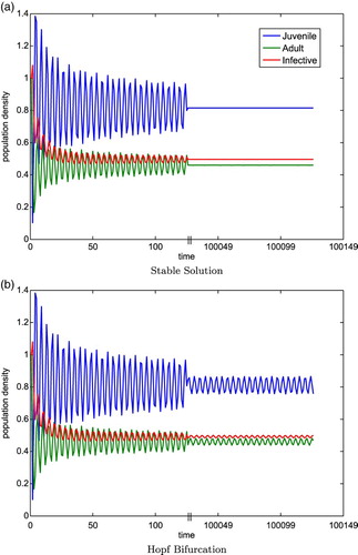
We present an example of a Hopf bifurcation that occurs somewhere between $\gamma =5.27$ and $5.28$ with $f_0=20$ and $s=0.54$. Note that in Table 1, ${\mathcal{E}}_2$ changes sign meaning that condition (iv) is first violated as proved in Lemma 4.2. Figure 1 (a) and 1 (b) are numerical solutions of System (35(34) $\begin{array}{rl}{J}_{t+1}\left(x\right)& ={\int }_{-\mathrm{\infty }}^{\mathrm{\infty }}{k}_{\mathrm{c}}(x-y)f\left(A_t\right(y\left)\right)\mathrm{d}y,\\ A_{t+1}\left(x\right)& =s\left(J_t\right(x)+A_t(x\left)\right)(1-T_{\mathrm{p}}(x\left)\right),\\ I_{t+1}\left(x\right)& =s\left(J_t\right(x)+A_t(x\left)\right)T_{\mathrm{p}}\left(x\right)+s{I}_t\left(x\right),\end{array}$(34) ) for these two sets of parameter values.

Table 1. An example of Hopf bifurcation.

γ	${\lambda }_1$	${\lambda }_2,{\overline{\lambda }}_2$	$\left|{\lambda }_2\right|$	$p\left(1\right)$
$5.27$	$0.9103$	$0.1490\pm 0.9888i$	$0.9999$	$0.1526$
$5.28$	$0.9109$	$0.1497\pm 0.9892i$	$1.0004$	$0.1517$
γ	$p(-1)$	${\mathcal{E}}_1$	${\mathcal{E}}_2$	${\mathcal{E}}_3$
$5.27$	$-4.3896$	$-0.0898$	$-0.0002$	$-0.2915$
$5.28$	$-4.3955$	$-0.0883$	$0.0014$	$-0.2900$

Notes: Parameter values $f_0=20$ and $s=0.54$. From Equations (48(45) ${\overline{\sigma }}_{t+1}=M\sum _{j=0}^{t-1}{s}^j+s^t{\overline{\sigma }}_0$(45) ), (49(46) $\left(\mathrm{i}\right)p\left(1\right)>0,$(46) ), and (50(47) $\left(\mathrm{ii}\right)p(-1)<0,$(47) ), we define ${\mathcal{E}}_1:=\left|a_3\right|-1$, ${\mathcal{E}}_2:=|a_2-a_1{a}_3|-|1-a_3^2|,$ and ${\mathcal{E}}_3:=|a_1-a_1{a}_3|-|a_2-a_1{a}_3+1-a_3^2|$. The results give an illustration to the result presented in Lemma 4.2.

Figure 1. The blue, green, and red curves correspond to the juvenile, adult, and infected classes, respectively. Parameter values: $f_0=20$, $s=0.54$, $\gamma =5.27$ for (a) and $\gamma =5.28$ for (b). The initial conditions are $J_0=A_0=I_0=1$. The first break occurs at $t=125$ and the plot continues at $t=100025$, denoted by the tick marks on the time axis. The steady state $E^{\ast }\approx (0.81465,0.46,0.49633)$. In the left plot, we can see that $E^{\ast }$ is stable and there is no Hopf bifurcation because $\gamma <{\gamma }^{\ast }$. In the right plot, a Hopf bifurcation occurs because $\gamma >{\gamma }^{\ast }$ with $E^{\ast }$ being unstable but there is a stable periodic solution which oscillates around $E^{\ast }$.

4.2. Simulations of the JAI model with dispersion

We now consider the JAI model with dispersion. There are two difficulties with studying System (34(33) $-\frac{v^2}{4D^2}+\frac{{\alpha }_{\mathrm{c}}}{D}\left(\frac{f_{0}sm}{(1-s)(1-s(1-m\left)\right)}-1\right)>0.$(33) ). First, the operator on the right is non-monotone due to overcompensation and the form of $T_{\mathrm{p}}$. Currently, there is no mathematical theory to determine the asymptotic spreading speed for non-monotone operators except in some special cases [15, 41]. Second, the model has a boundary steady state, $B^{\ast }$, which may result in the formation of stacked front solutions. The profile of a stacked front solution looks like a staircase of travelling wave fronts, hence the name stacked front. To the authors' knowledge, the idea of stacked fronts was first introduced in a 1977 paper by Fife and McLeod [8, Theorem 3.3] for a single nonlinear reaction–diffusion equation. The results of Fife and McCleod were later extended to systems by Roquejoffre et al. [33]. In 2011, Iida et al. proved the existence of stacked front solutions for an m-component cooperative system with equal diffusion coefficients and boundary equilibria [17]. However, all previous theoretical works on stacked fronts were done for partial differential equations. The proofs relied on the use of comparison functions, which were constructed from phase plane analysis. Since integro-difference equations are non-local operators and there is no phase plane analysis, theoretical proofs of the existence of stacked front solutions are still unavailable. In this subsection, we provide numerical simulations to show the existence of stacked front solutions for the JAI model.

We present simulations for the different types of behaviour according to Proposition 4.4. For all cases, we assume that the settling rate of crab larvae is ${\alpha }_{\mathrm{c}}=\frac{1}{50}$, meaning that on average it takes 50 days for the crab larvae to enter the juvenile stage and the settling rate for parasites is ${\alpha }_{\mathrm{p}}=\frac{1}{9}$, meaning that on average it takes 9 days for the parasites to find a host to infest. Also, advection is $v=0.85$ km/day and diffusion is $D=100{\mathrm{km}}^2/\mathrm{day}$.

Case (i): $f_0<1/s-1$. In this case, only $O^{\ast }$ exists and is stable. We prove that all solutions to System (34(33) $-\frac{v^2}{4D^2}+\frac{{\alpha }_{\mathrm{c}}}{D}\left(\frac{f_{0}sm}{(1-s)(1-s(1-m\left)\right)}-1\right)>0.$(33) ) converge to zero as $t\to \mathrm{\infty }$. The proof of this statement is outlined in Appendix 4 and hence simulations are not provided. Biologically, this is the desired case because the green crab population is completely eradicated. The only condition that must be satisfied for eradication of the green crab population is $f_0<1/s-1$.

Case (ii): $1/s-1<f_0<(1/s-1){\mathrm{e}}^{\gamma (1-s)}$. In this case $O^{\ast }$ and $B^{\ast }$ exist but not $E^{\ast }$. Furthermore, $O^{\ast }$ is unstable and $B^{\ast }$ is stable. Solutions to System (34(33) $-\frac{v^2}{4D^2}+\frac{{\alpha }_{\mathrm{c}}}{D}\left(\frac{f_{0}sm}{(1-s)(1-s(1-m\left)\right)}-1\right)>0.$(33) ) spreads with $\mathit{\beta }$ in Equations (A3(64) $m_{+}\left(z\right)=\frac{a_{{\mathrm{p}}_1}{a}_{{\mathrm{p}}_2}}{(z+a_{{\mathrm{p}}_1})(z+a_{{\mathrm{p}}_2})},$(64) ) and (A4(64) $m_{+}\left(z\right)=\frac{a_{{\mathrm{p}}_1}{a}_{{\mathrm{p}}_2}}{(z+a_{{\mathrm{p}}_1})(z+a_{{\mathrm{p}}_2})},$(64) ) being $B^{\ast }$ except that we do not have an explicit formula for $c_{\pm }^{\ast }$ 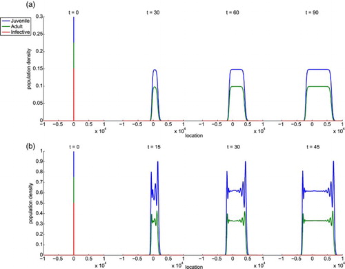so we make a formal conjecture to their values in Conjecture 4.6. A biological interpretation of Case (ii) is that the infected class dies out quickly and invasions of the juvenile and adult crabs continue to propagate. This case is not favourable in terms of S. carcini being an effective biological control agent because the parasite population does not persist. Figure 2 shows typical examples of solutions where $B^{\ast }$ is stable.

Figure 2. Simulations of System (34(33) $-\frac{v^2}{4D^2}+\frac{{\alpha }_{\mathrm{c}}}{D}\left(\frac{f_{0}sm}{(1-s)(1-s(1-m\left)\right)}-1\right)>0.$(33) ) when $B^{\ast }$ is stable. The blue, green, and red curves correspond to the juvenile, adult, and infected classes, respectively. In example (a) $f_0=3,s=0.4,\gamma =7,$ and $B^{\ast }\approx (0.1485,0.0990,0)$. In this case, there is no oscillation behind the wave front because the eigenvalues of the matrix $M_B$ defined in Proposition  4.4 are real valued: ${\lambda }_{\pm }\approx 0.6734,-0.2734$. In example (b) $f_0=19,s=0.35,\gamma =7,$ and $B^{\ast }\approx (0.6169,0.3322,0)$. The oscillatory behaviour of the solution in the tail of the wave front occurs because two of the eigenvalues of $M_B$ defined in Proposition 4.4 are complex valued: ${\lambda }_{\pm }\approx 0.1750\pm 0.9115i$ with $|{\lambda }_{\pm }|\approx 0.9282$. Note that in both examples, $c_{+}^{\ast }>c_{-}^{\ast }$ so the right front spreads faster as expected from the definition of $k{}_c{}_{\mathrm{c}}\left(x\right)$ in Equation (6(6) $\begin{array}{r}{k}_{\mathrm{c}}\left(x\right):=\frac{a_{{\mathrm{c}}_1}{a}_{{\mathrm{c}}_2}}{a_{{\mathrm{c}}_2}-a_{{\mathrm{c}}_1}}\left\{\begin{array}{l}{\mathrm{e}}^{a_{{\mathrm{c}}_1}x}x\le 0,,\\ {\mathrm{e}}^{a{}_{c_2}{}_{{\mathrm{c}}_2}x}& x>0,\end{array}\right.\end{array}$(6) ).

Conjecture 4.6.

Consider the system of equations given by System (34(33) $-\frac{v^2}{4D^2}+\frac{{\alpha }_{\mathrm{c}}}{D}\left(\frac{f_{0}sm}{(1-s)(1-s(1-m\left)\right)}-1\right)>0.$(33) ) with $1/s-1<f_0<(1/s-1){\mathrm{e}}^{\gamma (1-s)}$. We conjecture that the asymptotic spreading speed, $c_{\pm }^{\ast }$, for the juvenile and adult classes is given by formulas (21(21) $c_{+}^{\ast }=\underset{0<z<-a_{{\mathrm{c}}_2}}{min}\left[\frac{1}{z}\ln \left({\rho }_{+}\right(z\left)\right)\right]$(21) ) and (22(22) $c_{-}^{\ast }=\underset{0<z<a_{{\mathrm{c}}_1}}{min}\left[\frac{1}{z}\ln \left({\rho }_{-}\right(z\left)\right)\right],$(22) ) provided in Proposition 3.2 with $m=1$. Table 2 gives an example to support this conjecture.

Table 2. Numerical (JAI numerical and JA numerical) and analytical (Formulas (21(21) $c_{+}^{\ast }=\underset{0<z<-a_{{\mathrm{c}}_2}}{min}\left[\frac{1}{z}\ln \left({\rho }_{+}\right(z\left)\right)\right]$(21) ) and (22(22) $c_{-}^{\ast }=\underset{0<z<a_{{\mathrm{c}}_1}}{min}\left[\frac{1}{z}\ln \left({\rho }_{-}\right(z\left)\right)\right],$(22) )) results for the asymptotic spreading speed for two simulations of System (34(33) $-\frac{v^2}{4D^2}+\frac{{\alpha }_{\mathrm{c}}}{D}\left(\frac{f_{0}sm}{(1-s)(1-s(1-m\left)\right)}-1\right)>0.$(33) ), where $B^{\ast }$ is stable to support Conjecture 4.6.

$f_0=3,s=0.4,\gamma =7$	$c_{-}^{\ast }$	$c_{+}^{\ast }$
JAI numerical	29.8335	84.4159
JA numerical	29.8407	84.4273
Formulas (21(21) $c_{+}^{\ast }=\underset{0<z<-a_{{\mathrm{c}}_2}}{min}\left[\frac{1}{z}\ln \left({\rho }_{+}\right(z\left)\right)\right]$(21) ) and (22(22) $c_{-}^{\ast }=\underset{0<z<a_{{\mathrm{c}}_1}}{min}\left[\frac{1}{z}\ln \left({\rho }_{-}\right(z\left)\right)\right],$(22) )	30.3211	85.4008
$f_0=19,s=0.35,\gamma =7$	$c_{-}^{\ast }$	$c_{+}^{\ast }$
JAI numerical	86.8253	187.1559
JA numerical	86.8302	187.1655
Formulas (21(21) $c_{+}^{\ast }=\underset{0<z<-a_{{\mathrm{c}}_2}}{min}\left[\frac{1}{z}\ln \left({\rho }_{+}\right(z\left)\right)\right]$(21) ) and (22(22) $c_{-}^{\ast }=\underset{0<z<a_{{\mathrm{c}}_1}}{min}\left[\frac{1}{z}\ln \left({\rho }_{-}\right(z\left)\right)\right],$(22) )	88.5271	190.551

Notes: In the table, it is clear that the numerical results from the JA and JAI models agree but there is some discrepancy between the theoretical results and results from numerical simulations due to numerical errors in approximating convolution on a finite interval. Note that the numerical speeds calculated are always less than the theoretical speed.

Case (iii): $f_0>(1/s-1){\mathrm{e}}^{\gamma (1-s)}$. For the spatially independent case, a Hopf bifurcation may occur if $E^{\ast }$ becomes unstable. For example, if one considers the model given by System (34(33) $-\frac{v^2}{4D^2}+\frac{{\alpha }_{\mathrm{c}}}{D}\left(\frac{f_{0}sm}{(1-s)(1-s(1-m\left)\right)}-1\right)>0.$(33) ) with $f_0=20$ and $s=0.54$, then for $\gamma \le 5.27$, there is no Hopf bifurcation and $E^{\ast }$ is stable. For $\gamma \ge 5.28$ a Hopf bifurcation occurs forcing a stable periodic solution to appear about the unstable steady state $E^{\ast }$.

Another unique feature of this case is that stacked fronts can arise as a solution to System (34(33) $-\frac{v^2}{4D^2}+\frac{{\alpha }_{\mathrm{c}}}{D}\left(\frac{f_{0}sm}{(1-s)(1-s(1-m\left)\right)}-1\right)>0.$(33) ). When stacked front solutions occur, the leading front propagates with only the juvenile and adult classes whose tail converges to $B^{\ast }$, the parasite-free steady state. The trailing front propagates according to the slower moving infected class whose tail converges to $E^{\ast }$, the coexistence steady state. Figure 3 shows the results of three simulations to illustrate the different behaviour as described in the previous paragraphs. We formulate another conjecture about the asymptotic spreading speeds for the leading and trailing fronts.

Figure 3. The blue, green, and red curves correspond to the juvenile, adult, and infected classes, respectively. In example (a) $f_0=20$, $s=0.54$, and $\gamma =5.27$. This is the case where $E^{\ast }$ is stable so there is no Hopf bifurcation. The solution forms a stacked front with the leading front connecting $O^{\ast }$ to $B^{\ast }$ and the trailing front connects $B^{\ast }$ to $E^{\ast }$, where $B^{\ast }\approx (0.5102,0.5989,0)$ and $E^{\ast }\approx (0.8147,0.4600,0.4963)$. The leading front oscillates before converging to $B^{\ast }$ because two of the eigenvalues of $M_B$ are $\approx 0.2700\pm 0.9586i$ while the third is $\approx 1.1389$ clearly showing that $B^{\ast }$ is unstable. The eigenvalues of $M_E$ are ${\lambda }_{E\pm }\approx 0.1490\pm 0.9888i$ with $|{\lambda }_{E\pm }|\approx 0.9999$ and the third eigenvalue is $\approx 0.9103$. Thus, $E^{\ast }$ is stable. In example (b) $f_0=20$, $s=0.54$ and $\gamma =5.4$. This is the case where $E^{\ast }$ is unstable so there is a Hopf bifurcation. The solution also forms a stacked front. Here, $B^{\ast }\approx (0.4979,0.5845,0)$ and $E^{\ast }\approx (0.7674,0.4600,0.4408)$. We choose γ to be much larger than $5.27$ to make the bifurcated solution about $E^{\ast }$ more visible. We do not include the leading front in the plots for (b) because the behaviour is similar to example (a) and are more interested in the Hopf bifurcation. In example (c) $f_0=2.7187$, $s=0.3585$, and $\gamma =0.0825$. This is the case where $E^{\ast }$ is stable and there is no stacked front. It is clear that $B^{\ast }$ is unstable and $E^{\ast }$ is stable because the largest eigenvalue of $M_B$ is $\approx 5.4285$ and the eigenvalues of $M_E$ are ${\lambda }_{E\pm }\approx 0.9307\pm 0.2780i$, where $|{\lambda }_{E\pm }|\approx 0.9713$ and the third eigenvalue is $\approx -0.7234$.

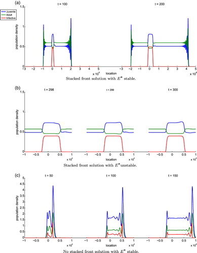
Conjecture 4.7.

Consider the system of equations given by System (34(33) $-\frac{v^2}{4D^2}+\frac{{\alpha }_{\mathrm{c}}}{D}\left(\frac{f_{0}sm}{(1-s)(1-s(1-m\left)\right)}-1\right)>0.$(33) ) with $f_0>(1/s-1){\mathrm{e}}^{\gamma (1-s)}$, where stacked front solutions occur. We conjecture that the asymptotic spreading speed for the leading front is given by those formulas in Proposition 3.2 with $m=1,$ while the asymptotic spreading speed for the trailing front is given by the following formulas: (62) $c_{+}^{\ast }=\underset{0<z<-a_{{\mathrm{p}}_2}}{min}\left[\frac{1}{z}\ln \left(s\right(B_J^{\ast }+B_A^{\ast }\left)m_{+}\right(z)+s)\right],$(62) (63) $c_{-}^{\ast }=\underset{0<z<+a_{{\mathrm{p}}_1}}{min}\left[\frac{1}{z}\ln \left(s\right(B_J^{\ast }+B_A^{\ast }\left)m_{-}\right(z)+s)\right],$(63) where (64) $m_{+}\left(z\right)=\frac{a_{{\mathrm{p}}_1}{a}_{{\mathrm{p}}_2}}{(z+a_{{\mathrm{p}}_1})(z+a_{{\mathrm{p}}_2})},$(64) (65) $m_{-}\left(z\right)=\frac{a_{{\mathrm{p}}_1}{a}_{{\mathrm{p}}_2}}{(z-a_{{\mathrm{p}}_1})(z-a_{{\mathrm{p}}_2})},$(65) and $B_J^{\ast },B_A^{\ast }$ are the $J,A$ components of $B^{\ast }$.

The reasoning behind Conjecture 4.7 is the following. Ahead of the leading front, there are no infected crabs and hence the juvenile and adult crabs propagate according to System (34(33) $-\frac{v^2}{4D^2}+\frac{{\alpha }_{\mathrm{c}}}{D}\left(\frac{f_{0}sm}{(1-s)(1-s(1-m\left)\right)}-1\right)>0.$(33) ) with $I_t=0$. These asymptotic spreading speeds are the same as those derived in model (10(11) $\begin{array}{rl}{J}_{t+1}& =s(1-m)J_t+f_0{\mathrm{e}}^{-\gamma A_t}{A}_t,\\ A_{t+1}& =sm{J}_t+s{A}_t.\end{array}$(11) ) with $m=1$. Ahead of the trailing front, $J_t=B_J^{\ast }$ and $A_t=B_A^{\ast }$. The linearization of the last equation of (34(33) $-\frac{v^2}{4D^2}+\frac{{\alpha }_{\mathrm{c}}}{D}\left(\frac{f_{0}sm}{(1-s)(1-s(1-m\left)\right)}-1\right)>0.$(33) ) about $B^{\ast }$ yields the equation (66) $I_{t+1}\left(x\right)=s(B_J^{\ast }+B_A^{\ast }){\int }_{-\mathrm{\infty }}^{\mathrm{\infty }}{k}_{\mathrm{p}}(x-y)I_t\left(y\right)\mathrm{d}y+s{I}_t\left(x\right).$(66) Formulas (62(56) $a_1=-\left(s+\frac{1}{\mu s}\right),$(56) ) and (63(57) $a_2=-\frac{1}{\mu }\left(\right(\mu -1\left)\right(1-\gamma (1-s))-1),$(57) ) follow from this observation and Proposition A.1. Table 3 provides some numerical results to support Conjecture 4.7. In the case where there is no stacked front, we make Conjecture 4.8 on the asymptotic spreading speed. Table 4 provides numerical support for this conjecture.

Table 3. Numerical (Leading Front JAI numerical, JA numerical, Trailing Front, JAI numerical, and I numerical) and analytical (Formulas (21(21) $c_{+}^{\ast }=\underset{0<z<-a_{{\mathrm{c}}_2}}{min}\left[\frac{1}{z}\ln \left({\rho }_{+}\right(z\left)\right)\right]$(21) ), (22(22) $c_{-}^{\ast }=\underset{0<z<a_{{\mathrm{c}}_1}}{min}\left[\frac{1}{z}\ln \left({\rho }_{-}\right(z\left)\right)\right],$(22) ), (62(56) $a_1=-\left(s+\frac{1}{\mu s}\right),$(56) ), and (63(57) $a_2=-\frac{1}{\mu }\left(\right(\mu -1\left)\right(1-\gamma (1-s))-1),$(57) )) results for the asymptotic spreading speed for simulations of System (34(33) $-\frac{v^2}{4D^2}+\frac{{\alpha }_{\mathrm{c}}}{D}\left(\frac{f_{0}sm}{(1-s)(1-s(1-m\left)\right)}-1\right)>0.$(33) ), where $E^{\ast }$ is stable and stacked front solutions exist where I numerical is a simulation of Equation (66(60) $\text{where}a=\frac{1}{3}(3a_2-a_1^2)\text{and}b=\frac{1}{27}(2a_1^3-9a_1{a}_2+27a_3).$(60) ). Both cases support Conjecture 4.7.

$f_0=20,s=0.54,\gamma =5.27$	$c_{-}^{\ast }$	$c_{+}^{\ast }$
Leading Front JAI numerical	103.2843	216.1826
JA numerical	103.2890	216.1926
Formulas (21(21) $c_{+}^{\ast }=\underset{0<z<-a_{{\mathrm{c}}_2}}{min}\left[\frac{1}{z}\ln \left({\rho }_{+}\right(z\left)\right)\right]$(21) ) and (22(22) $c_{-}^{\ast }=\underset{0<z<a_{{\mathrm{c}}_1}}{min}\left[\frac{1}{z}\ln \left({\rho }_{-}\right(z\left)\right)\right],$(22) )	105.4709	220.4714
Trailing Front JAI numerical	11.6324	21.9085
I numerical	11.6202	21.8809
Formulas (62(56) $a_1=-\left(s+\frac{1}{\mu s}\right),$(56) ) and (63(57) $a_2=-\frac{1}{\mu }\left(\right(\mu -1\left)\right(1-\gamma (1-s))-1),$(57) )	11.9567	22.4471

Notes: As in Table 2, the numerical speeds calculated are less than theoretical speeds because of numerical errors resulting from computing the convolutions over a finite interval.

Table 4. Numerical (JAI numerical and JA numerical) and analytical (Formulas (21(21) $c_{+}^{\ast }=\underset{0<z<-a_{{\mathrm{c}}_2}}{min}\left[\frac{1}{z}\ln \left({\rho }_{+}\right(z\left)\right)\right]$(21) ) and (22(22) $c_{-}^{\ast }=\underset{0<z<a_{{\mathrm{c}}_1}}{min}\left[\frac{1}{z}\ln \left({\rho }_{-}\right(z\left)\right)\right],$(22) )) results for the asymptotic spreading speed for simulations of System (34(33) $-\frac{v^2}{4D^2}+\frac{{\alpha }_{\mathrm{c}}}{D}\left(\frac{f_{0}sm}{(1-s)(1-s(1-m\left)\right)}-1\right)>0.$(33) ), where $E^{\ast }$ is stable and a single front propagates. We can see that the numeral results agree with the analytical results given by Conjecture 4.8. The relative errors for $c_{-}^{\ast }$ and $c_{+}^{\ast }$ for the JAI simulations are $1.67\mathrm{\%}$ and $1.01\mathrm{\%},$ respectively.

$f_0=2.7187$, $s=0.3585$, $\gamma =0.0825$	$c_{-}^{\ast }$	$c_{+}^{\ast }$
JAI numerical	$18.8762$	$66.3448$
JA numerical	$18.9047$	$66.3676$
Formulas (21(21) $c_{+}^{\ast }=\underset{0<z<-a_{{\mathrm{c}}_2}}{min}\left[\frac{1}{z}\ln \left({\rho }_{+}\right(z\left)\right)\right]$(21) ) and (22(22) $c_{-}^{\ast }=\underset{0<z<a_{{\mathrm{c}}_1}}{min}\left[\frac{1}{z}\ln \left({\rho }_{-}\right(z\left)\right)\right],$(22) )	$19.6770$	$67.6610$

Conjecture 4.8.

Consider the system of equations given by System (34(33) $-\frac{v^2}{4D^2}+\frac{{\alpha }_{\mathrm{c}}}{D}\left(\frac{f_{0}sm}{(1-s)(1-s(1-m\left)\right)}-1\right)>0.$(33) ) with $f_0>(1/s-1){\mathrm{e}}^{\gamma (1-s)}$ where only a single front propagates. Then the asymptotic spreading speed for the juvenile, adult, and infected classes is given by those formulas provided in Proposition 3.2 with $m=1$.

5. Conclusion and discussion

This paper presents a mathematical approach for studying the spatial spread of C. maenas, which has invaded the coastal regions of Northern America causing severe damage to the local ecosystem. The mathematical model presented takes the form of a system of discrete-time integral recursions (2(2) $\begin{array}{rl}{J}_{t+1}\left(x\right)& =s(1-m)(1-T_{\mathrm{p}}(x\left)\right)J_t\left(x\right)+{\int }_{-\mathrm{\infty }}^{\mathrm{\infty }}{k}_{\mathrm{c}}(x-y)f\left(A_t\right(y\left)\right)\mathrm{d}y,\\ A_{t+1}\left(x\right)& =sm(1-T_{\mathrm{p}}(x\left)\right)J_t\left(x\right)+s(1-T_{\mathrm{p}}(x\left)\right)A_t\left(x\right),\\ I_{t+1}\left(x\right)& =sm{T}_{\mathrm{p}}\left(x\right)J_t\left(x\right)+s{T}_{\mathrm{p}}\left(x\right)A_t\left(x\right)+s_{\mathrm{p}}{I}_t\left(x\right).\end{array}$(2) ). The spatial spread of the crabs is modelled using dispersal kernels, which includes the effects of diffusion and advection of coastal current with a constant settling rate. We consider a control strategy by introducing a castrating parasite, S. carcini, and explore the population dynamics of the European green crab.

The primary results presented in this paper are the formulas for the asymptotic spreading speeds and the classification of solutions behaviour. For model (10(11) $\begin{array}{rl}{J}_{t+1}& =s(1-m)J_t+f_0{\mathrm{e}}^{-\gamma A_t}{A}_t,\\ A_{t+1}& =sm{J}_t+s{A}_t.\end{array}$(11) ), we are able to provide theoretical formulas. However, for model (34(33) $-\frac{v^2}{4D^2}+\frac{{\alpha }_{\mathrm{c}}}{D}\left(\frac{f_{0}sm}{(1-s)(1-s(1-m\left)\right)}-1\right)>0.$(33) ), we can only make conjectures on the asymptotic spreading speeds and provide numerical evidence to support our conjectures. The classifications for the behaviour of solutions provide easy conditions to determine the type of solution one would expect for a particular set of parameter values.

The results in this paper clearly demonstrate the need to develop mathematical tools to analyse models in non-homogeneous environments and non-monotone operators. This is seen in Conjectures 4.6–4.8. There is also need for mathematical theory of existence of stacked front solutions for non-local operators such as integro-difference equations.

The JA model only has two steady states, the extirpation steady state and the non-trivial steady state. We proved that the population will persist if and only if condition (14(14) $f_0>\frac{(1-s)(1-s(1-m\left)\right)}{sm}.$(14) ) is satisfied. This simple inequality can be checked easily for a given set of parameter values. Thus, the model predicts that the green crabs will either grow to capacity or become extirpated.

For the JA model we are able to use the theory for asymptotic spreading speeds for monotone operators to derive formulas for the spread of green crab without inclusion of the parasite dynamics as a biological control. Therefore, without the parasites the crabs spread up and down the coast causing damage to the ecosystem. As expected from the choice of dispersal kernel, the formulas for the asymptotic spreading speed predict that the crabs travel faster in the direction of the advection (downstream). We showed that the downstream speed for the green crab spread is always positive. This means that the green crab will continue to spread until there is no remaining viable habitat to invade. We were also able to show that under certain conditions, for example, very strong advection, the green crab cannot spread upstream. In this case, the upstream green crab population would not continue to spread upstream but instead the population would collapse upon itself. To further understand which parameters most affect the asymptotic spreading speed, one could perform a sensitivity analysis of $c_{\pm }^{\ast }$. For an easy read on how to perform sensitivity analysis, see [29].

The JAI model includes the introduction of the castrating parasite, S. carcini, as a biological control agent. The dynamics of this model are much more complicated than the JA model. The model has three steady states: $O^{\ast }$ the extirpation steady state, $B^{\ast }$ the parasite-free steady state, and $E^{\ast }$ the coexistence steady state. The ecological interpretations of Proposition 4.4 are as follows.

Case (i): When $f_0<1/s-1$, the extirpation steady state is stable and the parasite-free and coexistence steady states do not exist. It is interesting to see that the eradication condition only depends on $f_0$ and s, not the amount of infected crabs in the system. Thus, if we are looking to eradicate an established local green crab population, a control measure that affects the linearized fecundity ($f_0$) and/or survival probability (s) should be used.

Case (ii): When $1/s-1<f_0<(1/s-1){\mathrm{e}}^{\gamma (1-s)}$ the extirpation steady state is unstable, the parasite-free steady state is stable, and the coexistence steady state does not exist. Thus, the juvenile and adult classes will spread and the entire infected class will die. We hypothesize that the population will spread according to Equations (21(21) $c_{+}^{\ast }=\underset{0<z<-a_{{\mathrm{c}}_2}}{min}\left[\frac{1}{z}\ln \left({\rho }_{+}\right(z\left)\right)\right]$(21) ) and (22(22) $c_{-}^{\ast }=\underset{0<z<a_{{\mathrm{c}}_1}}{min}\left[\frac{1}{z}\ln \left({\rho }_{-}\right(z\left)\right)\right],$(22) ) as done in the JA model. Thus, as explained in the JA model, the crab population will always spread downstream and if there is strong enough advection then the upstream population front will also spread downstream.

Case (iii): When $f_0>(1/s-1){\mathrm{e}}^{\gamma (1-s)}$ the extirpation and parasite-free steady states are unstable. The coexistence steady state is stable if $\gamma <{\gamma }^{\ast }$ and a Hopf bifurcation occurs otherwise. One interesting case of System (34(33) $-\frac{v^2}{4D^2}+\frac{{\alpha }_{\mathrm{c}}}{D}\left(\frac{f_{0}sm}{(1-s)(1-s(1-m\left)\right)}-1\right)>0.$(33) ) is that all constant steady state solutions exist but are unstable and Hopf bifurcation occurs. This idea is well understood mathematically. Another interesting case is the existence of stacked front solutions of System (34(33) $-\frac{v^2}{4D^2}+\frac{{\alpha }_{\mathrm{c}}}{D}\left(\frac{f_{0}sm}{(1-s)(1-s(1-m\left)\right)}-1\right)>0.$(33) ). It is well known that stacked front solutions can only occur if a boundary steady state exists. In our case, the only boundary steady state is the parasite-free steady state and we see that the juvenile and adult populations will always outrun the infected population when stacked front solutions occur. This suggests that the use of S. carcini as a biological control agent would not be effective if introduced at a single point in time, because the juvenile and adult populations will always outrun the infected crab population.

There are some limitations of the model presented in this paper that should be addressed. The introduction of S. carcini could have severe impact on the native crab species. The interactions between the native crab and S. carcini need to be fully explored before making any decisions about the effectiveness of the parasite as a biological control agent. Second, we do not explore the relationship between C. maenas and native species. Including competition between the different species for resources may change the dynamics of the population growth and spread of C. maenas. Also, we do not model S. carcini directly in the present model. Including an equation for the parasite population over time could allow one to derive a more general model. The use of S. carcini as a biological control agent raises another issue because it is not species specific to C. maenas [22]. In our model, there is no consideration on how S. carcini affects other native crab populations. This problem needs to be studied before determining the effectiveness of S. carcini as a biological control in terms of risk assessment.

The model we studied is one dimensional in space. C. maenas is also known as the common shore crab because of affinity for living in shallow water, 5–6  m, but has been found in depths of up to 60  m [4]. This restriction on the crabs' habitat allows for us to make the simplifying assumption that the population only spreads up and down the coast. It is known that the green crab also moves in and out of shore due to tides. An incorporation of this aspect into the model would add another spatial dimension and would require a different time scale. The model also assumes that the coastline is infinitely long in order to apply the mathematical theory of asymptotic spreading speed. This is a reasonable assumption because the distance the green crab spread is short compared to the length of the coastline. Another assumption is that the demographic and dispersal parameters in the model are assumed to be independent of location. Including these effects will result in an operator that is non-homogeneous; that is, it does not commute with translations.

The order of biological events is important in understanding models defined by mathematical recursions. For our model, we perform census of the population at time t, the crabs then reproduce followed by the larvae dispersing. Finally, the crabs mature and survive to the next generation before the next censusing occurs. To obtain data to validate the model, censusing of crab densities should be collected after dispersal when the number of larvae is small.

Acknowledgments

The problem of modelling C. maenas was first introduced to the first author (NGM) at the 2013 PIMS IGTC Mathematical Biology Summer School on The Mathematics Behind Biological Invasions being held at the University of Alberta. We would like to thank the organizers, Mark Lewis and Thomas Hillen, for giving NGM the opportunity to attend the programme, to Dr Lewis for his guidance during the initial development of the project, and to the participants Andrew Bateman, Andreas Buttenschön, Devin Goodsman, and Kelley Erickson for their help in the initial development of a more general model.

Disclosure statement

No potential conflict of interest was reported by the authors.

Appendix 1. Asymptoticspreading speed for a system

The following proposition is taken from [23]. Let $\mathit{\beta }\in {\mathbb{R}}^n$ be a positive vector. We define $\begin{array}{rl}\mathcal{C}& =\{\mathbf{\text{u}}=(u^1,\dots ,u^n)|\mathbf{\text{0}}\le \mathbf{\text{u}}(x)\le \mathit{\beta },u^i(x):\mathbb{R}\to [0,{\mathit{\beta }}^i]\\ & \text{is piecewise continuous for}i=1,\dots ,n\}.\end{array}$

Proposition .1.

Let $\mathbf{Q}=(Q^1,\dots ,Q^n):\mathcal{C}\to \mathcal{C}$ satisfy the following conditions:

1. $\mathbf{Q}\left[\mathbf{0}\right]=\mathbf{0},\mathbf{Q}\left[\mathit{\beta }\right]=\mathit{\beta }$, $\mathbf{0}$ is unstable and $\mathit{\beta }$ is stable with respect to $\mathbf{Q}$.

2. $\mathbf{Q}$ is translation invariant and has no other fixed point besides $\mathbf{0}$ and $\mathit{\beta }$ in $\mathcal{C}$.

3. $\mathbf{Q}$ is monotone or order-preserving in $\mathcal{C};$ that is, if $\mathbf{u}\le \mathbf{v}$ in $\mathcal{C},$ then $\mathbf{Q}\left[\mathbf{u}\right]\le \mathbf{Q}\left[\mathbf{v}\right]$.

4. $\mathbf{Q}$ is continuous in the topology of uniform convergence on bounded subsets of $\mathbb{R}$.

5. Let $\left(\mathbf{M}\right[\mathbf{u}\left]\right(x){)}_i=\sum _{j=1}^n{\int }_{-\mathrm{\infty }}^{\mathrm{\infty }}{\mathbf{u}}_j(x-y\left)m^{ij}\right(y)\mathrm{d}y$ be the linearization of $\mathbf{Q}$ at $\mathbf{0},$ where $m^{ij}\left(y\right)\ge 0$ is an integrable function. We assume that (A1) $\mathbf{Q}\left[\mathbf{u}\right]\le \mathbf{M}\left[\mathbf{u}\right]\text{for all}\mathbf{u}\in \mathcal{C}.$(A1)

6. The matrix $B_{\pm }\left(z\right)=\left(b_{\pm }^{ij}\right(z\left)\right),$ where $b_{\pm }^{ij}\left(z\right)={\int }_{-\mathrm{\infty }}^{\mathrm{\infty }}{\mathrm{e}}^{\pm zy}{m}^{ij}\left(y\right)\mathrm{d}y$ is irreducible for $0<z<z_{\pm }$.

Let ${\rho }_{\pm }\left(z\right)$ be the spectral radius of $B_{\pm }\left(z\right)$ and let (A2) $c_{\pm }^{\ast }=\underset{\begin{array}{c}0<z<z_{\pm }\end{array}}{min}\frac{1}{z}\ln {\rho }_{\pm }\left(z\right).$(A2) Then $c_{\pm }^{\ast }$ are the asymptotic spreading speeds of the operator $\mathbf{Q}$ in the positive and negative directions, respectively, in the following sense. Let ${\mathbf{u}}_0\in \mathcal{C},$ ${\mathbf{u}}_0$ is non-trivial and vanishes outside of a bounded interval in $\mathbb{R}$. Let ${\mathbf{u}}_t$ be defined by ${\mathbf{u}}_{t+1}=\mathbf{Q}\left[{\mathbf{u}}_t\right]$ for $t=0,1,2\dots$. Suppose $-c_{-}^{\ast }<c_{+}^{\ast }$. Then for any small $\epsilon >0,$ (A3) $\begin{array}{rl}& \underset{t\to \mathrm{\infty }}{lim}\underset{x\in [-t(c_{-}^{\ast }-\epsilon ),t(c_{+}^{\ast }-\epsilon \left)\right]}{min}|{\mathbf{u}}_t\left(x\right)-\mathit{\beta }|=0\end{array}$(A3) (A4) $\begin{array}{rl}\text{and}& \underset{t\to \mathrm{\infty }}{lim}\underset{x\notin [-t(c_{-}^{\ast }+\epsilon ),t(c_{+}^{\ast }+\epsilon \left)\right]}{max}|{\mathbf{u}}_t\left(x\right)|=0.\end{array}$(A4)

Appendix 2. Proof of Lemma 4.2

Proof.

Condition (i) or (ii) cannot be violated first because that would mean the pair of complex eigenvalues that leaves the unit circle first is not satisfied. Condition (iii) cannot be violated first because suppose $|a_3|=1$. Then conditions (iv) and (v) are also violated with $a_2=a_1{a}_3$ and $a_1=a_2{a}_3$. If $a_3=\eta /\mu =1$, then $\gamma (1-s)f_0{\mathrm{e}}^{-\gamma (1-s)}=-1$, which is a contradiction. If $a_3=\eta /\mu =-1$, then $a_1=-a_2$, which implies that $-(s+1/\mu s)=\eta -1/\mu =-1-1/\mu$. Simplifying, we have $\mu s=1$, also a contradiction. It remains to show that condition (v) cannot be violated first. Suppose the strict inequality in Equation (50(47) $\left(\mathrm{ii}\right)p(-1)<0,$(47) ) is replaced by equality. Because of Equation (48(45) ${\overline{\sigma }}_{t+1}=M\sum _{j=0}^{t-1}{s}^j+s^t{\overline{\sigma }}_0$(45) ), condition (iv) becomes $|a_2-a_1{a}_3|<1-a_3^2$. Therefore, the term inside the absolute value on the right side of Equation (50(47) $\left(\mathrm{ii}\right)p(-1)<0,$(47) ) is non-negative, yielding either $a_1-a_2{a}_3=a_2-a_1{a}_3+1-a_3^2\text{or}-(a_1-a_2{a}_3)=a_2-a_1{a}_3+1-a_3^2.$ Rearranging and simplifying, we have $p(-1)=-1+a_1-a_2+a_3=0\text{or}p\left(1\right)=1+a_1+a_2+a_3=0.$ Therefore, either condition (46(43) $f_0>1/s-1.$(43) ) or (47(44) ${\sigma }_{t+1}=f_0{\mathrm{e}}^{-\gamma A_t}{A}_t+s{\sigma }_t\le M+s{\sigma }_t.$(44) ) is violated. The proof of the lemma is complete.

Appendix 3. Proof of Lemma 4.3

Proof.

In this calculation, $f_0$ and s are constant and μ is the bifurcation parameter. Recall that $\mu =f_0{\mathrm{e}}^{-\gamma (1-s)}+1$ and $\eta =(\mu -1)(\delta +\ln (\mu -1\left)\right)$, where $\delta =1-\ln f_0$. Then ${\eta }_{\mu }=1+\eta /(\mu -1)$ and $(a_3{)}_{\mu }={\left(\frac{\eta }{\mu }\right)}_{\mu }=\frac{1}{\mu }+\frac{a_3}{\mu (\mu -1)}.$ If condition (iv) were the first to be violated, we can write it as $a_2-a_1{a}_3=1-a_3^2$ because if $a_2-a_1{a}_3<0$, then the expression inside the absolute value on the right of Equation (50(47) $\left(\mathrm{ii}\right)p(-1)<0,$(47) ) is zero, yielding a contradiction. Let $g\left(\mu \right):=a_2-a_1{a}_3-1+a_3^2=\frac{1}{\mu }-a_3-a_1{a}_3-1+a_3^2.$ Recall that $a_1=-s-1/\left(\mu s\right)$. Then $(a_1{)}_{\mu }=1/({\mu }^{2}s)$ and $g^{\mathrm{\prime }}\left(\mu \right)=-(1+a_1-2a_3)\left(\frac{1}{\mu }+\frac{a_3}{\mu (\mu -1)}\right)-\frac{1}{{\mu }^2}\left(1+\frac{a_3}{s}\right).$ Suppose $g\left({\mu }^{\ast }\right)=g^{\mathrm{\prime }}\left({\mu }^{\ast }\right)=0$. From above, we have $({\mu }^{\ast }-1)(1+a_1-2a_3)=\left(1-\frac{1}{{\mu }^{\ast }}+a_3+a_1{a}_3\right)-\frac{{\mu }^{\ast }-1}{{\mu }^{\ast }}\left(\frac{a_3}{s}\right).$ Solving for $a_3$ from this equation and equating the result to the definition of $a_3$, we have $\begin{array}{rl}{a}_3& =\frac{{\mu }^{\ast }-1}{{\mu }^{\ast }}\left(\delta +\ln ({\mu }^{\ast }-1)\right)\\ & =\frac{({\mu }^{\ast }-1)\left[\right(s^2-s){\mu }^{\ast }+(1+s\left)\right]}{{\mu }^{\ast }\left(-2{\mu }^{\ast }s+s+s^2+1\right)}.\end{array}$ The proof of the lemma is complete.

Appendix 4. Proof of Case (i)

Proof.

Let $({\overline{J}}_t,{\overline{A}}_t)$ be the solutions of System (34(33) $-\frac{v^2}{4D^2}+\frac{{\alpha }_{\mathrm{c}}}{D}\left(\frac{f_{0}sm}{(1-s)(1-s(1-m\left)\right)}-1\right)>0.$(33) ) with $I_t=0$ in the second equation, and let $(J_0,A_0)\le ({\overline{J}}_0,{\overline{A}}_0)$. Then one can show that $(J_t,A_t)\le ({\overline{J}}_t,{\overline{A}}_t)$ for all t. Let $({\overline{J}}_0,{\overline{A}}_0)$ be a constant vector. Then so are $({\overline{J}}_t.{\overline{A}}_t)$ for $t\ge 1$, which satisfy the recursion ${\overline{A}}_{t+1}=s{f}_0{\mathrm{e}}^{-\gamma {\overline{A}}_{t-1}}{\overline{A}}_{t-1}+s{\overline{A}}_t.$ Since $f_0<1/s-1$, ${\overline{A}}_t$ is dominated by the sequence $\left\{a_t\right\}$, which satisfies the recursion $a_{t+1}=\theta (1-s)a_{t-1}+s{a}_t,\theta =\frac{s{f}_0}{1-s}\in (0,1).$ Let $a_t=r^t$. Then r satisfies $r^2-c_{1}r-c_2=0$, where $c_1=s$ and $c_2=\theta (1-s)$. The roots of this quadratic equation are $r_1=\frac{1}{2}\left(c_1+\sqrt{c_1^2+4c_2}\right),r_2=\frac{1}{2}\left(c_1-\sqrt{c_1^2+4c_2}\right).$ Since $0<c_1+c_2<1$, we have $|r_i|<1,i=1,2$. Thus, $a_t\to 0$ as $t\to \mathrm{\infty }$. The proof is complete.

References

- N.S. Banas, P.S. McDonald, and D.A. Armstrong, Green crab larval retention in Willapa Bay, Washington: An intensive Lagrangian modeling approach, Estuar. Coast. 32 (2009), pp. 893–905. doi: 10.1007/s12237-009-9175-7
- C.J.A. Bradshaw and C.R. McMahon, Population ecology: Fecundity, in Encyclopedia of Ecology, S.E. Jørgensen and B.D. Fath, eds., Elsevier, Oxford, 2008, pp. 1535–1543.
- J.E. Byers and J.M. Pringle, Going against the flow: Retention, range limits and invasions in advective environments, Mar. Ecol. Prog. Ser. 313 (2006), pp. 27–41. doi: 10.3354/meps313027
- A.N. Cohen, J.T. Carlton, and M.C. Fountain, Introduction, dispersal and potential impacts of the green crab Carcinus maenas in San Francisco Bay, California, Mar. Biol. 122 (1995), pp. 225–237.
- R.I. Colautti, S.A. Bailey, C.D.A. Overdijkvon, K. Amundsen, and H.J. MacIsaac, Characterised and projected costs of nonindigenous species in Canada, Biol. Invasions 8 (2006), pp. 45–59. doi: 10.1007/s10530-005-0236-y
- R.C. Davis and F.T. Short, Restoring eelgrass, Zostera marina l., habitat using a new transplanting technique: The horizontal rhizome method, Aquat. Botany 59 (1997), pp. 1–15. doi: 10.1016/S0304-3770(97)00034-X
- L. Edelstein-Keshet, Mathematical Models in Biology, SIAM, Philadelphia, PA, 2005.
- P.C. Fife and J.B. McLeod, The approach of solutions of nonlinear diffusion equations to travelling front solutions, Arch. Ration. Mech. Anal. 65 (1977), pp. 335–361. doi: 10.1007/BF00250432
- T. Floyd and J. Williams, Impact of green crab (Carcinus maenas l.) predation on a population of soft-shell clams (Mya arenaria l.) in the Southern Gulf of St. Lawrence, J. Shellfish Res. 23 (2004), pp. 457–462.
- J.B. Glude, The effects of temperature and predators on the abundance of the soft-shell clam, Mya arenaria, in New England, Trans. Am. Fisheries Soc. 84 (1955), pp. 13–26. doi: 10.1577/1548-8659(1954)84[13:TEOTAP]2.0.CO;2
- J.H. Goddard, M.E. Torchin, A.M. Kuris, and K.D. Lafferty, Host specificity of Sacculina carcini, a potential biological control agent of the introduced European green crab Carcinus maenas in California, Biol. Invasions 7 (2005), pp. 895–912. doi: 10.1007/s10530-003-2981-0
- E.D. Grosholz, Contrasting rates of spread for introduced species in terrestrial and marine systems, Ecology 77 (1996), pp. 1680–1686. doi: 10.2307/2265773
- E.D. Grosholz, G.M. Ruiz, C.A. Dean, K.A. Shirley, J.L. Maron, and P.G. Connors, The impacts of a nonindigenous marine predator in a California bay, Ecology 81 (2000), pp. 1206–1224. doi: 10.1890/0012-9658(2000)081[1206:TIOANM]2.0.CO;2
- J. Heavilin and J. Powell, A novel method of fitting spatio-temporal models to data, with applications to the dynamics of mountain pine beetles, Nat. Resour. Model. 21 (2008), pp. 489–524. doi: 10.1111/j.1939-7445.2008.00021.x
- S.-B. Hsu and X.-Q. Zhao, Spreading speeds and traveling waves for nonmonotone integrodifference equations, SIAM J. Math. Anal. 40 (2008), pp. 776–789. doi: 10.1137/070703016
- H.L. Hunt and L.S. Mullineaux, The roles of predation and postlarval transport in recruitment of the soft shell clam (Mya arenaria), Limnol. Oceanogr. 47 (2002), pp. 151–164. doi: 10.4319/lo.2002.47.1.0151
- M. Iida, R. Lui, and H. Ninomiya, Stacked fronts for cooperative systems with equal diffusion coefficients, SIAM J. Math. Anal. 43 (2011), pp. 1369–1389. doi: 10.1137/100792846
- L. Kanary, J. Musgrave, R.C. Tyson, A. Locke, and F. Lutscher, Modelling the dynamics of invasion and control of competing green crab genotypes, Theor. Ecol. 7 (2014), pp. 391–406. doi: 10.1007/s12080-014-0226-8
- G. Klassen and A. Locke, A biological synopsis of the European green crab, Carcinus maenas, Canadian Manuscript Report of Fisheries and Aquatic Sciences, 2007.
- M. Kot, Discrete-time traveling waves: Ecological examples, J. Math. Biol. 30 (1992), pp. 413–436. doi: 10.1007/BF00173295
- M. Kot, M.A. Lewis, and P. Driesschevan den, Dispersal data and the spread of invading organisms, Ecology 77 (1996), pp. 2027–2042. doi: 10.2307/2265698
- A.M. Kuris, K.D. Lafferty, and M.E. Torchin, Biological control of the European green crab, Carcinus maenas: Natural enemy evaluation and analysis of host specificity, 2nd International Symposium Biological Control of Arthropods, Davos, 2005.
- R. Lui, Biological growth and spread modeled by systems of recursions. I. Mathematical theory, Math. Biosci. 93 (1989), pp. 269–295. doi: 10.1016/0025-5564(89)90026-6
- F. Lutscher, E. Pachepsky, and M.A. Lewis, The effect of dispersal patterns on stream populations, SIAM Rev. 47 (2005), pp. 749–772. doi: 10.1137/050636152
- S.P. McDonald, G.C. Jensen, and D.A. Armstrong, The competitive and predatory impacts of the nonindigenous crab Carcinus maenas (L.) on early benthic phase Dungeness crab Cancer magister Dana, J. Exp. Mar. Biol. Ecol. 258 (2001), pp. 39–54. doi: 10.1016/S0022-0981(00)00344-0
- S.H. Miller and S.G. Morgan, Temporal variation in cannibalistic infanticide by the shore crab Hemigrapsus oregonensis: Implications for reproductive success, Mar. Ecol. 36 (2015), pp. 842–847.
- P.-O. Moksnes, Self-regulating mechanisms in cannibalistic populations of juvenile shore crabs Carcinus maenas, Ecology 85 (2004), pp. 1343–1354. doi: 10.1890/02-0750
- T.F. Nalepa and D.W. Schloesser, Zebra Mussels: Biology, Impacts, and Control, CRC Press, Boca Raton, FL, 1992.
- M.G. Neubert and H. Caswell, Demography and dispersal: Calculation and sensitivity analysis of invasion speed for structured populations, Ecology 81 (2000), pp. 1613–1628. doi: 10.1890/0012-9658(2000)081[1613:DADCAS]2.0.CO;2
- J. Pineda, Linking larval settlement to larval transport: Assumptions, potentials, and pitfalls, Oceanogr. Eastern Pacific 1 (2000), pp. 84–105.
- G. Rilov and J.A. Crooks, Biological Invasions in Marine Ecosystems: Ecological, Management, and Geographic Perspectives, Springer, Berlin, 2008.
- J. Roman, Diluting the founder effect: Cryptic invasions expand a marine invader's range, Proc. Roy. Soc. B: Biol. Sci. 273 (2006), pp. 2453–2459. doi: 10.1098/rspb.2006.3597
- J.-M. Roquejoffre, D. Terman, and V.A. Volpert, Global stability of traveling fronts and convergence towards stacked families of waves in monotone parabolic systems, SIAM J. Math. Anal. 27 (1996), pp. 1261–1269. doi: 10.1137/S0036141094267522
- R.J. Sacker, Introduction to the 2009 re-publication of the ‘Neimark-Sacker bifurcation theorem’, J. Differ. Equ. Appl. 15 (2009), pp. 753–758. doi: 10.1080/10236190802357750
- E. Stokstad, Biologists rush to protect great lakes from onslaught of carp, Science 327 (2010), pp. 932. doi: 10.1126/science.327.5968.932
- D.L. Taylor, Predatory impact of the green crab (Carcinus maenas Linnaeus) on post-settlement winter flounder (Pseudopleuronectes americanus Walbaum) as revealed by immunological dietary analysis, J. Exp. Mar. Biol. Ecol. 324 (2005), pp. 112–126. doi: 10.1016/j.jembe.2005.04.014
- R.E. Thresher, M. Werner, J.T. Hoeg, I. Svane, H. Glenner, N. Murphy, and C. Wittwer, Developing the options for managing marine pests: Specificity trials on the parasitic castrator, Sacculina carcini, against the European crab, Carcinus maenas, and related species, J. Exp. Mar. Biol. Ecol. 254 (2000), pp. 37–51. doi: 10.1016/S0022-0981(00)00260-4
- M.E. Torchin, K.D. Lafferty, and A.M. Kuris, Release from parasites as natural enemies: Increased performance of a globally introduced marine crab, Biol. Invasions 3 (2001), pp. 333–345. doi: 10.1023/A:1015855019360
- R.W. Van Kirk and M.A. Lewis, Integrodifference models for persistence in fragmented habitats, Bull. Math. Biol. 59 (1997), pp. 107–137. doi: 10.1007/BF02459473
- M.-H. Wang, M. Kot, and M.G. Neubert, Integrodifference equations, Allee effects, and invasions, J. Math. Biol. 44 (2002), pp. 150–168. doi: 10.1007/s002850100116
- H.F. Weinberger, K. Kawasaki, and N. Shigesada, Spreading speeds of spatially periodic integro-difference models for populations with nonmonotone recruitment functions, J. Math. Biol. 57 (2008), pp. 387–411. doi: 10.1007/s00285-008-0168-0