On the principle of host evolution in host–pathogen interactions

ABSTRACT

In this paper, we use a two-host one pathogen immuno-epidemiological model to argue that the principle for host evolution, when the host is subjected to a fatal disease, is minimization of the case fatality proportion $\mathcal{F}$. This principle is valid whether the disease is chronic or leads to recovery. In the case of continuum of hosts, stratified by their immune response stimulation rate a, we suggest that $\mathcal{F}\left(a\right)$ has a minimum because a trade-off exists between virulence to the host induced by the pathogen and virulence induced by the immune response. We find that the minimization of the case fatality proportion is an evolutionary stable strategy for the host.

KEYWORDS:

• Immuno-epidemiology
• within-host dynamics
• age-since-infection
• multi-host
• competitive exclusion
• reproduction numbers
• virulence

1. Introduction

Pathogen evolution, and specifically the evolution of virulence, have been studied extensively through mathematical models with the early models assuming some kind of trade-off between virulence and transmission [7,11,13,20,21,25]. A competitive exclusion principle, suggesting that pathogens evolve to maximize their epidemiological reproduction number, was first rigorously established by Bremermann and Thieme [12]. This principle lead the way into the following studies on pathogen evolution and to the fundamental idea that pathogens evolve to some optimal virulence, that maximizes the reproduction number.

Studies in evolutionary genetics show that hosts, including humans, in turn, evolve under the selective pressure exhorted by the pathogen [6]. Mathematical models have investigated the evolution of host resistance [8,9,16,24]. Bowers [9] derived a principle for host evolution, similar to the reproduction number. His principle states that the host evolves towards minimizing a dimensionless quantity called the basic depression number $D_0$.

Anderson and May are the pioneers in the mathematical study of co-evolution of pathogens and hosts [3]. Early models of co-evolution, reviewed in [28], were mostly systems of ordinary differential equations (ODEs). In 2002, Gilchrist and Sasaki proposed a novel model of ‘nested’ dynamical immunological model into an epidemiological model [17]. Since then nested immuno-epidemiological models have become a primary tool in the study of evolution of pathogens [1,2,4,5,14,15,19]. Gilchrist and Sasaki, in fact, studied the co-evolution of the pathogen and the host. They used the lifespan of the host in the infectious class as a criterion for host evolution, assuming no natural mortality. Pugliese [26] later showed analytically that, even in the presence of natural mortality, the host evolves towards maximizing its lifespan in the infectious class. This measure, however, is not adequate for immuno-epidemiological models that model diseases with recovery. Why would the host strive to extend its lifespan in the infectious class, if it has an option to recover?

The purpose of this note is to extend the criterion for host evolution to immuno-epidemiological models with recovery. We argue that the host evolves towards minimizing the case fatality proportion $\mathcal{F}$. The case fatality proportion in immuno-epidemiological models is given by $\mathcal{F}={\int }_0^{\mathrm{\infty }}\alpha \left(\tau \right)\pi \left(\tau \right)\mathrm{d}\tau ,$ where $\alpha \left(\tau \right)$ is the disease-induced death rate and $\pi \left(\tau \right)$ is the probability of survival in the infectious class. In the ODE case the case fatality proportion is given by $\mathcal{F}=\frac{\alpha }{\alpha +\gamma +m_0},$ where γ is the recovery rate and $m_0$ is the natural death rate. The case fatality proportion gives the fraction of the individuals who die from the disease. In epidemiology, $\mathcal{F}$ is called case fatality ratio (CFR). Our measure is in a sense a special case of the one derived by Bowers and assumes that all hosts have the same reproduction rate and the same natural death rate, that is, we assume that these host characteristics do not evolve under the pressure of the pathogen [9]. We further consider the case fatality proportion $\mathcal{F}\left(a\right)$ as a function of the immune response activation rate a and argue that the case fatality proportion has a minimum because a trade-off exists between the virulence generated by the pathogen and the virulence generated by the immune response. Using tools from adaptive dynamics, we show that minimizing the case fatality proportion is an evolutionary stable strategy (ESS) for the host.

This paper is organized as follows. In the next section, we introduce a two-host immuno-epidemiological model. We link the epidemiological parameters to the within-host dynamic variables [17]. We derive the basic reproduction number. In Section 3 we compute the equilibria of the model and determine their stabilities. We show that host one equilibrium is stable if host one minimizes the case fatality proportion. If host one has the smallest case fatality proportion, the stability of host one equilibrium is established in several particular cases. In Section 4 we consider simulations with a continuum of hosts, stratified by their immune response stimulation rate $\mathcal{F}\left(a\right)$ and we show that $\mathcal{F}\left(a\right)$ has a minimum. Section 5 summarizes our results.

2. A two-host immuno-epidemiological model

In this section we formulate a two-host immuno-epidemiological model which models directly transmitted diseases with recovery, such as Hepatitis C Virus, influenza and foot-and-mouth disease. Both hosts have the same recruitment rate and natural mortality but vary in susceptibility, recovery rate and disease-induced mortality (virulence). Both hosts experience different within-host dynamics, given by a standard immunological single-strain model.

2.1. The within-host model

Within a host, the time variable is denoted by τ and signifies time-since-infection. We model only the pathogen and the immune response, denoted, respectively, by $P_i\left(\tau \right)$ and $B_i\left(\tau \right)$. The pathogen reproduces linearly at a rate $r_i$ and is killed by the immune response with efficacy ${ϵ}_i$. The pathogen stimulates the immune response at a rate $a_i$. The within-host model for host i takes the form [17]: (1) $\text{Within-host Model:}\left\{\begin{array}{ll}\frac{\mathrm{d}{P}_i}{\mathrm{d}\tau }& =r_i{P}_i\left(\tau \right)-{ϵ}_i{B}_i\left(\tau \right)P_i\left(\tau \right),\\ \frac{\mathrm{d}{B}_i}{\mathrm{d}\tau }& =a_i{P}_i\left(\tau \right)B_i\left(\tau \right).\end{array}\right.$(1)

This model is equipped with initial conditions $P_i\left(0\right)=P_0$ and $B_i\left(0\right)=B_0$.

All parameters and dependent variables of this within-host model and their definitions can be found in Table 1.

Table 1. List of parameters and variables.

Notation	Meaning
$P\left(\tau \right)$	Pathogen concentration at time-since infection τ
$B\left(\tau \right)$	Antibody concentration at time-since infection τ
r	Pathogen growth rate
ε	Efficiency of the antibodies killing the pathogen
a	Antibody activation rate

This model has a very simple dynamics. Within a host, if $r/\left(ϵB\right(0\left)\right)>1$ the pathogen takes off, reaches a maximum and then declines to zero. The immune response increases and levels off. If $r/\left(ϵB\right(0\left)\right)<1$, the pathogen decreases to zero.

Dividing the two equations in (1(1) $\text{Within-host Model:}\left\{\begin{array}{ll}\frac{\mathrm{d}{P}_i}{\mathrm{d}\tau }& =r_i{P}_i\left(\tau \right)-{ϵ}_i{B}_i\left(\tau \right)P_i\left(\tau \right),\\ \frac{\mathrm{d}{B}_i}{\mathrm{d}\tau }& =a_i{P}_i\left(\tau \right)B_i\left(\tau \right).\end{array}\right.$(1) ), we can obtain P as a function of B, (2) $P=\frac{1}{a}\left(r\ln \frac{B}{B_0}-ϵ(B-B_0)+a{P}_0\right).$(2) Using the second equation in (1(1) $\text{Within-host Model:}\left\{\begin{array}{ll}\frac{\mathrm{d}{P}_i}{\mathrm{d}\tau }& =r_i{P}_i\left(\tau \right)-{ϵ}_i{B}_i\left(\tau \right)P_i\left(\tau \right),\\ \frac{\mathrm{d}{B}_i}{\mathrm{d}\tau }& =a_i{P}_i\left(\tau \right)B_i\left(\tau \right).\end{array}\right.$(1) ), we obtain the following differential equation for B: (3) $B^{\prime }\left(\tau \right)=B\left(r\ln \frac{B}{B_0}-ϵ(B-B_0)+a{P}_0\right).$(3) This is a separable equation but it is still hard to solve exactly because of the complexity of the right-hand side.

2.2. The between-host model

In this subsection we introduce a two-host epidemiological model. The two hosts are subjected to a unique pathogen. We denote by $S_j\left(t\right)$ the number of susceptible individuals of host type j at time t. We structure the infected individuals by time-since-infection τ. Let $i_j(\tau ,t)$ be the density of infected individuals of host type j. Individuals in the class $i_j(\tau ,t)$ experience the same within-host dynamics given by model (1(1) $\text{Within-host Model:}\left\{\begin{array}{ll}\frac{\mathrm{d}{P}_i}{\mathrm{d}\tau }& =r_i{P}_i\left(\tau \right)-{ϵ}_i{B}_i\left(\tau \right)P_i\left(\tau \right),\\ \frac{\mathrm{d}{B}_i}{\mathrm{d}\tau }& =a_i{P}_i\left(\tau \right)B_i\left(\tau \right).\end{array}\right.$(1) ) for host type j. We assume the epidemiological dynamics is given by the following two-host model: (4) $\begin{array}{rl}\frac{\mathrm{d}{S}_1}{\mathrm{d}t}& =N_{1}b\left(N\right)-S_1\left(t\right){\int }_0^{\mathrm{\infty }}{\beta }_1\left(\tau \right)i_1(\tau ,t)\mathrm{d}\tau -S_1\left(t\right){\int }_0^{\mathrm{\infty }}{\beta }_2\left(\tau \right)i_2(\tau ,t)\mathrm{d}\tau -m_0{S}_1,\\ \frac{\mathrm{\partial }{i}_1}{\mathrm{\partial }\tau }+\frac{\mathrm{\partial }{i}_1}{\mathrm{\partial }t}& =-(m_0+{\alpha }_1(\tau )+{\gamma }_1(\tau \left)\right)i_1(\tau ,t),\\ i_1(0,t)& =S_1\left(t\right){\int }_0^{\mathrm{\infty }}{\beta }_1\left(\tau \right)i_1(\tau ,t)\mathrm{d}\tau +S_1\left(t\right){\int }_0^{\mathrm{\infty }}{\beta }_2\left(\tau \right)i_2(\tau ,t)\mathrm{d}\tau ,\\ \frac{\mathrm{d}{R}_1}{\mathrm{d}t}& ={\int }_0^{\mathrm{\infty }}{\gamma }_1\left(\tau \right)i_1(\tau ,t)\mathrm{d}\tau -m_0{R}_1,\\ \frac{\mathrm{d}{S}_2}{\mathrm{d}t}& =N_{2}b\left(N\right)-S_2\left(t\right){\int }_0^{\mathrm{\infty }}{\beta }_1\left(\tau \right)i_1(\tau ,t)\mathrm{d}\tau -S_2\left(t\right){\int }_0^{\mathrm{\infty }}{\beta }_2\left(\tau \right)i_2(\tau ,t)\mathrm{d}\tau -m_0{S}_2,\\ \frac{\mathrm{\partial }{i}_2}{\mathrm{\partial }\tau }+\frac{\mathrm{\partial }{i}_2}{\mathrm{\partial }t}& =-(m_0+{\alpha }_2(\tau )+{\gamma }_2(\tau \left)\right)i_2(\tau ,t),\\ i_2(0,t)& =S_2\left(t\right){\int }_0^{\mathrm{\infty }}{\beta }_1\left(\tau \right)i_1(\tau ,t)\mathrm{d}\tau +S_2\left(t\right){\int }_0^{\mathrm{\infty }}{\beta }_2\left(\tau \right)i_2(\tau ,t)\mathrm{d}\tau ,\\ \frac{\mathrm{d}{R}_2}{\mathrm{d}t}& ={\int }_0^{\mathrm{\infty }}{\gamma }_2\left(\tau \right)i_2(\tau ,t)\mathrm{d}\tau -m_0{R}_2.\end{array}$(4)

In model (4(4) $\begin{array}{rl}\frac{\mathrm{d}{S}_1}{\mathrm{d}t}& =N_{1}b\left(N\right)-S_1\left(t\right){\int }_0^{\mathrm{\infty }}{\beta }_1\left(\tau \right)i_1(\tau ,t)\mathrm{d}\tau -S_1\left(t\right){\int }_0^{\mathrm{\infty }}{\beta }_2\left(\tau \right)i_2(\tau ,t)\mathrm{d}\tau -m_0{S}_1,\\ \frac{\mathrm{\partial }{i}_1}{\mathrm{\partial }\tau }+\frac{\mathrm{\partial }{i}_1}{\mathrm{\partial }t}& =-(m_0+{\alpha }_1(\tau )+{\gamma }_1(\tau \left)\right)i_1(\tau ,t),\\ i_1(0,t)& =S_1\left(t\right){\int }_0^{\mathrm{\infty }}{\beta }_1\left(\tau \right)i_1(\tau ,t)\mathrm{d}\tau +S_1\left(t\right){\int }_0^{\mathrm{\infty }}{\beta }_2\left(\tau \right)i_2(\tau ,t)\mathrm{d}\tau ,\\ \frac{\mathrm{d}{R}_1}{\mathrm{d}t}& ={\int }_0^{\mathrm{\infty }}{\gamma }_1\left(\tau \right)i_1(\tau ,t)\mathrm{d}\tau -m_0{R}_1,\\ \frac{\mathrm{d}{S}_2}{\mathrm{d}t}& =N_{2}b\left(N\right)-S_2\left(t\right){\int }_0^{\mathrm{\infty }}{\beta }_1\left(\tau \right)i_1(\tau ,t)\mathrm{d}\tau -S_2\left(t\right){\int }_0^{\mathrm{\infty }}{\beta }_2\left(\tau \right)i_2(\tau ,t)\mathrm{d}\tau -m_0{S}_2,\\ \frac{\mathrm{\partial }{i}_2}{\mathrm{\partial }\tau }+\frac{\mathrm{\partial }{i}_2}{\mathrm{\partial }t}& =-(m_0+{\alpha }_2(\tau )+{\gamma }_2(\tau \left)\right)i_2(\tau ,t),\\ i_2(0,t)& =S_2\left(t\right){\int }_0^{\mathrm{\infty }}{\beta }_1\left(\tau \right)i_1(\tau ,t)\mathrm{d}\tau +S_2\left(t\right){\int }_0^{\mathrm{\infty }}{\beta }_2\left(\tau \right)i_2(\tau ,t)\mathrm{d}\tau ,\\ \frac{\mathrm{d}{R}_2}{\mathrm{d}t}& ={\int }_0^{\mathrm{\infty }}{\gamma }_2\left(\tau \right)i_2(\tau ,t)\mathrm{d}\tau -m_0{R}_2.\end{array}$(4) ), $N_{j}b\left(N\right)$ is the birth/recruitment rate where $N_j=S_j+{\int }_0^{\mathrm{\infty }}{i}_j(\tau ,t)\mathrm{d}\tau +R_j$ is the total population size of host j and $N=N_1+N_2$ is the total population size of both hosts. $b\left(N\right)$ is a function of N such that $b^{\prime }\left(N\right)<0$ for all N and $b^{-1}\left(m_0\right)$ exists. Furthermore, $b\left(0\right)=b_0$. In addition, $m_0$ is the natural death rate and ${\alpha }_j\left(\tau \right)$ is the disease-induced death rate of host type j. We will assume the simplest form of ${\alpha }_j\left(\tau \right)$, that is, ${\alpha }_j\left(\tau \right)={\sigma }_j{P}_j\left(\tau \right)+{\xi }_j{B}_j\left(\tau \right),$ where ${\sigma }_j{P}_j\left(\tau \right)$ represents host mortality due to the pathogen and ${\xi }_j{B}_j\left(\tau \right)$ gives the additional host mortality due to the immune response. We note that other forms of disease-induced mortality rate are possible [17]. The transmission coefficient ${\beta }_j\left(\tau \right)$ is also dependent on the within-host pathogen load. We may assume that ${\beta }_j\left(\tau \right)$ is Holling type II with respect to the pathogen load at a given time-since-infection τ. Hence, ${\beta }_j\left(\tau \right)=\frac{c_j{P}_j\left(\tau \right)}{d_j+P_j\left(\tau \right)},$ where $P_j\left(\tau \right)$ is the viral load in host type j, $d_j$ is the half-saturation constant and $c_j$ is proportionality constant. The recovery rate is directly proportional to the immune response $B_j$ and inversely related to the viral load. Hence, ${\gamma }_j\left(\tau \right)=\frac{{\kappa }_j{B}_j}{{ϵ}_0+P_j\left(\tau \right)},$ where ${\kappa }_j$ is proportionality constant and ${ϵ}_0$ is a small number.

Model (4(4) $\begin{array}{rl}\frac{\mathrm{d}{S}_1}{\mathrm{d}t}& =N_{1}b\left(N\right)-S_1\left(t\right){\int }_0^{\mathrm{\infty }}{\beta }_1\left(\tau \right)i_1(\tau ,t)\mathrm{d}\tau -S_1\left(t\right){\int }_0^{\mathrm{\infty }}{\beta }_2\left(\tau \right)i_2(\tau ,t)\mathrm{d}\tau -m_0{S}_1,\\ \frac{\mathrm{\partial }{i}_1}{\mathrm{\partial }\tau }+\frac{\mathrm{\partial }{i}_1}{\mathrm{\partial }t}& =-(m_0+{\alpha }_1(\tau )+{\gamma }_1(\tau \left)\right)i_1(\tau ,t),\\ i_1(0,t)& =S_1\left(t\right){\int }_0^{\mathrm{\infty }}{\beta }_1\left(\tau \right)i_1(\tau ,t)\mathrm{d}\tau +S_1\left(t\right){\int }_0^{\mathrm{\infty }}{\beta }_2\left(\tau \right)i_2(\tau ,t)\mathrm{d}\tau ,\\ \frac{\mathrm{d}{R}_1}{\mathrm{d}t}& ={\int }_0^{\mathrm{\infty }}{\gamma }_1\left(\tau \right)i_1(\tau ,t)\mathrm{d}\tau -m_0{R}_1,\\ \frac{\mathrm{d}{S}_2}{\mathrm{d}t}& =N_{2}b\left(N\right)-S_2\left(t\right){\int }_0^{\mathrm{\infty }}{\beta }_1\left(\tau \right)i_1(\tau ,t)\mathrm{d}\tau -S_2\left(t\right){\int }_0^{\mathrm{\infty }}{\beta }_2\left(\tau \right)i_2(\tau ,t)\mathrm{d}\tau -m_0{S}_2,\\ \frac{\mathrm{\partial }{i}_2}{\mathrm{\partial }\tau }+\frac{\mathrm{\partial }{i}_2}{\mathrm{\partial }t}& =-(m_0+{\alpha }_2(\tau )+{\gamma }_2(\tau \left)\right)i_2(\tau ,t),\\ i_2(0,t)& =S_2\left(t\right){\int }_0^{\mathrm{\infty }}{\beta }_1\left(\tau \right)i_1(\tau ,t)\mathrm{d}\tau +S_2\left(t\right){\int }_0^{\mathrm{\infty }}{\beta }_2\left(\tau \right)i_2(\tau ,t)\mathrm{d}\tau ,\\ \frac{\mathrm{d}{R}_2}{\mathrm{d}t}& ={\int }_0^{\mathrm{\infty }}{\gamma }_2\left(\tau \right)i_2(\tau ,t)\mathrm{d}\tau -m_0{R}_2.\end{array}$(4) ) is equipped with the following initial conditions: $S_j\left(0\right)=S_j^0$, $i_j(\tau ,0)={\varphi }_j\left(\tau \right)$ and $R_j\left(0\right)=R_j^0$ with j=1,2. All parameters are nonnegative and $c_j>0$, $m_0>0$.

The epidemiological reproduction number of host type j in system (4(4) $\begin{array}{rl}\frac{\mathrm{d}{S}_1}{\mathrm{d}t}& =N_{1}b\left(N\right)-S_1\left(t\right){\int }_0^{\mathrm{\infty }}{\beta }_1\left(\tau \right)i_1(\tau ,t)\mathrm{d}\tau -S_1\left(t\right){\int }_0^{\mathrm{\infty }}{\beta }_2\left(\tau \right)i_2(\tau ,t)\mathrm{d}\tau -m_0{S}_1,\\ \frac{\mathrm{\partial }{i}_1}{\mathrm{\partial }\tau }+\frac{\mathrm{\partial }{i}_1}{\mathrm{\partial }t}& =-(m_0+{\alpha }_1(\tau )+{\gamma }_1(\tau \left)\right)i_1(\tau ,t),\\ i_1(0,t)& =S_1\left(t\right){\int }_0^{\mathrm{\infty }}{\beta }_1\left(\tau \right)i_1(\tau ,t)\mathrm{d}\tau +S_1\left(t\right){\int }_0^{\mathrm{\infty }}{\beta }_2\left(\tau \right)i_2(\tau ,t)\mathrm{d}\tau ,\\ \frac{\mathrm{d}{R}_1}{\mathrm{d}t}& ={\int }_0^{\mathrm{\infty }}{\gamma }_1\left(\tau \right)i_1(\tau ,t)\mathrm{d}\tau -m_0{R}_1,\\ \frac{\mathrm{d}{S}_2}{\mathrm{d}t}& =N_{2}b\left(N\right)-S_2\left(t\right){\int }_0^{\mathrm{\infty }}{\beta }_1\left(\tau \right)i_1(\tau ,t)\mathrm{d}\tau -S_2\left(t\right){\int }_0^{\mathrm{\infty }}{\beta }_2\left(\tau \right)i_2(\tau ,t)\mathrm{d}\tau -m_0{S}_2,\\ \frac{\mathrm{\partial }{i}_2}{\mathrm{\partial }\tau }+\frac{\mathrm{\partial }{i}_2}{\mathrm{\partial }t}& =-(m_0+{\alpha }_2(\tau )+{\gamma }_2(\tau \left)\right)i_2(\tau ,t),\\ i_2(0,t)& =S_2\left(t\right){\int }_0^{\mathrm{\infty }}{\beta }_1\left(\tau \right)i_1(\tau ,t)\mathrm{d}\tau +S_2\left(t\right){\int }_0^{\mathrm{\infty }}{\beta }_2\left(\tau \right)i_2(\tau ,t)\mathrm{d}\tau ,\\ \frac{\mathrm{d}{R}_2}{\mathrm{d}t}& ={\int }_0^{\mathrm{\infty }}{\gamma }_2\left(\tau \right)i_2(\tau ,t)\mathrm{d}\tau -m_0{R}_2.\end{array}$(4) ) is given by the following expression: (5) ${\mathcal{R}}_j=b^{-1}\left(m_0\right){\int }_0^{\mathrm{\infty }}{\beta }_j\left(\tau \right){\mathrm{e}}^{-m_0\tau -{\int }_0^{\tau }\left({\alpha }_j\right(\sigma )+{\gamma }_j(\sigma \left)\right)\mathrm{d}\sigma }\mathrm{d}\tau ,j=1,2.$(5) The reproduction number of host type j gives the number of secondary infections that one type j-infected individual will produce in an entirely susceptible type j population during its lifespan as infectious. This is the reproduction number of the single-host model and does not depend on the interaction between the hosts.

In the next section we compute explicit expressions for the equilibria and establish their local stability.

3. Equilibria and their local stability

System (4(4) $\begin{array}{rl}\frac{\mathrm{d}{S}_1}{\mathrm{d}t}& =N_{1}b\left(N\right)-S_1\left(t\right){\int }_0^{\mathrm{\infty }}{\beta }_1\left(\tau \right)i_1(\tau ,t)\mathrm{d}\tau -S_1\left(t\right){\int }_0^{\mathrm{\infty }}{\beta }_2\left(\tau \right)i_2(\tau ,t)\mathrm{d}\tau -m_0{S}_1,\\ \frac{\mathrm{\partial }{i}_1}{\mathrm{\partial }\tau }+\frac{\mathrm{\partial }{i}_1}{\mathrm{\partial }t}& =-(m_0+{\alpha }_1(\tau )+{\gamma }_1(\tau \left)\right)i_1(\tau ,t),\\ i_1(0,t)& =S_1\left(t\right){\int }_0^{\mathrm{\infty }}{\beta }_1\left(\tau \right)i_1(\tau ,t)\mathrm{d}\tau +S_1\left(t\right){\int }_0^{\mathrm{\infty }}{\beta }_2\left(\tau \right)i_2(\tau ,t)\mathrm{d}\tau ,\\ \frac{\mathrm{d}{R}_1}{\mathrm{d}t}& ={\int }_0^{\mathrm{\infty }}{\gamma }_1\left(\tau \right)i_1(\tau ,t)\mathrm{d}\tau -m_0{R}_1,\\ \frac{\mathrm{d}{S}_2}{\mathrm{d}t}& =N_{2}b\left(N\right)-S_2\left(t\right){\int }_0^{\mathrm{\infty }}{\beta }_1\left(\tau \right)i_1(\tau ,t)\mathrm{d}\tau -S_2\left(t\right){\int }_0^{\mathrm{\infty }}{\beta }_2\left(\tau \right)i_2(\tau ,t)\mathrm{d}\tau -m_0{S}_2,\\ \frac{\mathrm{\partial }{i}_2}{\mathrm{\partial }\tau }+\frac{\mathrm{\partial }{i}_2}{\mathrm{\partial }t}& =-(m_0+{\alpha }_2(\tau )+{\gamma }_2(\tau \left)\right)i_2(\tau ,t),\\ i_2(0,t)& =S_2\left(t\right){\int }_0^{\mathrm{\infty }}{\beta }_1\left(\tau \right)i_1(\tau ,t)\mathrm{d}\tau +S_2\left(t\right){\int }_0^{\mathrm{\infty }}{\beta }_2\left(\tau \right)i_2(\tau ,t)\mathrm{d}\tau ,\\ \frac{\mathrm{d}{R}_2}{\mathrm{d}t}& ={\int }_0^{\mathrm{\infty }}{\gamma }_2\left(\tau \right)i_2(\tau ,t)\mathrm{d}\tau -m_0{R}_2.\end{array}$(4) ) has several disease-free equilibria.

1. $E_0=(0,0,0,0,0,0)$ which always exists.

2. $E_{01}=(S_1^{\left(1\right)},0,0,0,0,0)$ where $S_1^{\left(1\right)}=b^{-1}\left(m_0\right)$. This equilibrium exists if and only if $b_0>m_0$.

3. $E_{02}=(0,0,0,S_2^{\left(2\right)},0,0)$ where $S_2^{\left(2\right)}=b^{-1}\left(m_0\right)$. This equilibrium exists if and only if $b_0>m_0$.

4. There is also one parameter family of coexistence equilibria $E_{03}=(S_1^{\left(3\right)},0,0,S_2^{\left(3\right)},0,0)$ satisfying $S_1^{\left(3\right)}+S_2^{\left(3\right)}=b^{-1}\left(m_0\right).$

Before we introduce the host type j equilibria, we define the probability for survival in the jth infected class, ${\pi }_j\left(\tau \right)={\mathrm{e}}^{-{\int }_0^{\tau }(m_0+{\alpha }_j(\sigma )+{\gamma }_j(\tau \left)\right)\mathrm{d}\sigma }.$

If the basic reproduction number ${\mathcal{R}}_j>1$, for each j there is a corresponding single host infected equilibrium $E_j$ given by

1. $E_1=(S_1^{\ast },i_1^{\ast }(\tau ),R_1^{\ast },0,0,0)$

2. $E_2=(0,0,0,S_2^{\ast },i_2^{\ast }(\tau ),R_2^{\ast })$.

where $\begin{array}{rl}{S}_j^{\ast }& =\frac{b^{-1}\left(m_0\right)}{{\mathcal{R}}_j},\\ i_j^{\ast }\left(\tau \right)& =i_j^{\ast }\left(0\right){\pi }_j\left(\tau \right),\\ i_j^{\ast }\left(0\right)& =N_j^{\ast }b\left(N_j^{\ast }\right)-m_0{S}_j^{\ast },\\ R_j^{\ast }& =\frac{i_j^{\ast }\left(0\right){\int }_0^{\mathrm{\infty }}{\gamma }_j\left(\tau \right){\pi }_j\left(\tau \right)\mathrm{d}\tau }{m_0}\end{array}$ and $N_j^{\ast }$ is the solution of the following equation: (6) $N_j^{\ast }=S_j^{\ast }+K_j\left(\frac{N_j^{\ast }b\left(N_j^{\ast }\right)}{m_0}-S_j^{\ast }\right)$(6) and $K_j$ is given by the following constant: $K_j=m_0{\int }_0^{\mathrm{\infty }}{\pi }_j\left(\tau \right)\mathrm{d}\tau +{\int }_0^{\mathrm{\infty }}{\gamma }_j\left(\tau \right){\pi }_j\left(\tau \right)\mathrm{d}\tau .$

This claim merits justification. We formulate the result in the following proposition:

Proposition 3.1.

Assume ${\mathcal{R}}_j>1$. Then there exists a unique host type j equilibrium $E_j,$ where $E_1=(S_1^{\ast },i_1^{\ast }(\tau ),R_1^{\ast },0,0,0)$ and $E_2=(0,0,0,S_2^{\ast },i_2^{\ast }(\tau ),R_2^{\ast })$.

Proof.

We need to show that Equation (6(6) $N_j^{\ast }=S_j^{\ast }+K_j\left(\frac{N_j^{\ast }b\left(N_j^{\ast }\right)}{m_0}-S_j^{\ast }\right)$(6) ) has a unique solution satisfying $N_j^{\ast }>S_j^{\ast }$. If $N_j^{\ast }>S_j^{\ast }$, then the expression in the parenthesis is positive and, therefore, $i_j\left(0\right)>0$. Hence the equilibrium $E_j$ has only positive components for host type j. Given the properties of b, it is not hard to see that Equation (6(6) $N_j^{\ast }=S_j^{\ast }+K_j\left(\frac{N_j^{\ast }b\left(N_j^{\ast }\right)}{m_0}-S_j^{\ast }\right)$(6) ) always has a unique positive solution.

To see that $N_j^{\ast }>S_j^{\ast }$, we rewrite Equation (6(6) $N_j^{\ast }=S_j^{\ast }+K_j\left(\frac{N_j^{\ast }b\left(N_j^{\ast }\right)}{m_0}-S_j^{\ast }\right)$(6) ) as $N_j^{\ast }\left(1-K_j\frac{b\left(N_j^{\ast }\right)}{m_0}\right)=(1-K_j)S_j^{\ast },$ where we note that $K_j<1$. The left-hand side of this equation is a function of $N_j$, say $f\left(N_j\right)$. Since $f\left(N_j\right)$ is an increasing function of $N_j$, if the above equation has a solution, it is unique. To see the above equation has a solution satisfying $N_j^{\ast }>S_j^{\ast }$, notice that $f\left(S_j^{\ast }\right)<S_j^{\ast }(1-K_j),$ which follows from the fact that ${\mathcal{R}}_j>1$ and therefore, $b\left(S_j^{\ast }\right)>m_0$. Let ${\overline{N}}_j>S_j^{\ast }$ be such that $b\left({\overline{N}}_j\right)=m_0$. Then, $f\left({\overline{N}}_j\right)={\overline{N}}_j(1-K_j)>S_j^{\ast }(1-K_j).$ Hence, Equation (6(6) $N_j^{\ast }=S_j^{\ast }+K_j\left(\frac{N_j^{\ast }b\left(N_j^{\ast }\right)}{m_0}-S_j^{\ast }\right)$(6) ) has a unique solution in the interval $(S_j^{\ast },{\overline{N}}_j)$. This concludes the proof.

Next, we investigate the local stability of equilibria. First, we consider the extinction equilibrium. In the case of the extinction equilibrium, we state the following result which is not hard to prove.

Proposition 3.2.

The extinction equilibrium $E_0$ is locally asymptotically stable, if $b_0<m_0$ and unstable if $b_0>m_0$.

The stability of the disease-free boundary equilibria is given by the following proposition whose proof will also be omitted.

Proposition 3.3.

Equilibrium $E_{0j},j=1,2$ is neutrally stable $($principle eigenvalue is zero$)$ if ${\mathcal{R}}_j<1$ and unstable if ${\mathcal{R}}_j>1$.

We state the stability of the one parameter family of coexistence equilibria in the following proposition. We first denote $\stackrel{\mathcal{ˆ}}{\mathcal{R}}=S_1^{\left(3\right)}{\int }_0^{\mathrm{\infty }}{\beta }_1\left(\tau \right){\pi }_1\left(\tau \right)\mathrm{d}\tau +S_2^{\left(3\right)}{\int }_0^{\mathrm{\infty }}{\beta }_2\left(\tau \right){\pi }_2\left(\tau \right)\mathrm{d}\tau .$

Proposition 3.4.

Equilibrium $E_{03}$ is locally asymptotically stable if $\stackrel{\mathcal{ˆ}}{\mathcal{R}}<1$ and unstable if $\stackrel{\mathcal{ˆ}}{\mathcal{R}}>1$.

Next we establish the stability of $E_1$. Stability of $E_2$ is similar. The main result, the stability of $E_1$, gives conditions for the outcome of the competition of hosts one and two. It is well known that the outcome of the competition of multiple strains where competitive exclusion is the only outcome, is governed by the reproduction number – the strain with the maximal reproduction number eliminates the rest [12]. Here we establish that the competition between hosts, subject to the same pathogen, is governed by the case fatality proportion, defined as follows: (7) ${\mathcal{F}}_j={\int }_0^{\mathrm{\infty }}{\alpha }_j\left(s\right){\pi }_j\left(s\right)\mathrm{d}s.$(7) We note that ${\mathcal{F}}_j<1$. The case fatality proportion governs the outcome of the competition in both chronic diseases and diseases leading to recovery. Pugliese [26] suggested a different measure that governs the outcome of host competition, the lifespan in the infected class, but this measure is valid only if ${\gamma }_j\left(\tau \right)=0$, that is, recovery is impossible.

Stability of $E_1$ will give the criterion for the outcome of host competition. However, stability $E_1$ depends on two components (1) internal stability of the endemic equilibrium of a host one only system and (2) criterion for non-invasion of host two. In system (4(4) $\begin{array}{rl}\frac{\mathrm{d}{S}_1}{\mathrm{d}t}& =N_{1}b\left(N\right)-S_1\left(t\right){\int }_0^{\mathrm{\infty }}{\beta }_1\left(\tau \right)i_1(\tau ,t)\mathrm{d}\tau -S_1\left(t\right){\int }_0^{\mathrm{\infty }}{\beta }_2\left(\tau \right)i_2(\tau ,t)\mathrm{d}\tau -m_0{S}_1,\\ \frac{\mathrm{\partial }{i}_1}{\mathrm{\partial }\tau }+\frac{\mathrm{\partial }{i}_1}{\mathrm{\partial }t}& =-(m_0+{\alpha }_1(\tau )+{\gamma }_1(\tau \left)\right)i_1(\tau ,t),\\ i_1(0,t)& =S_1\left(t\right){\int }_0^{\mathrm{\infty }}{\beta }_1\left(\tau \right)i_1(\tau ,t)\mathrm{d}\tau +S_1\left(t\right){\int }_0^{\mathrm{\infty }}{\beta }_2\left(\tau \right)i_2(\tau ,t)\mathrm{d}\tau ,\\ \frac{\mathrm{d}{R}_1}{\mathrm{d}t}& ={\int }_0^{\mathrm{\infty }}{\gamma }_1\left(\tau \right)i_1(\tau ,t)\mathrm{d}\tau -m_0{R}_1,\\ \frac{\mathrm{d}{S}_2}{\mathrm{d}t}& =N_{2}b\left(N\right)-S_2\left(t\right){\int }_0^{\mathrm{\infty }}{\beta }_1\left(\tau \right)i_1(\tau ,t)\mathrm{d}\tau -S_2\left(t\right){\int }_0^{\mathrm{\infty }}{\beta }_2\left(\tau \right)i_2(\tau ,t)\mathrm{d}\tau -m_0{S}_2,\\ \frac{\mathrm{\partial }{i}_2}{\mathrm{\partial }\tau }+\frac{\mathrm{\partial }{i}_2}{\mathrm{\partial }t}& =-(m_0+{\alpha }_2(\tau )+{\gamma }_2(\tau \left)\right)i_2(\tau ,t),\\ i_2(0,t)& =S_2\left(t\right){\int }_0^{\mathrm{\infty }}{\beta }_1\left(\tau \right)i_1(\tau ,t)\mathrm{d}\tau +S_2\left(t\right){\int }_0^{\mathrm{\infty }}{\beta }_2\left(\tau \right)i_2(\tau ,t)\mathrm{d}\tau ,\\ \frac{\mathrm{d}{R}_2}{\mathrm{d}t}& ={\int }_0^{\mathrm{\infty }}{\gamma }_2\left(\tau \right)i_2(\tau ,t)\mathrm{d}\tau -m_0{R}_2.\end{array}$(4) ) what is difficult to prove and may not hold for all parameter values is (1). In the theorem below, we first establish the criterion for non-invasion, assuming (1).

Theorem 3.5.

Assume the endemic equilibrium of host one only system is locally asymptotically stable. Then, the equilibrium $E_1$ is locally asymptotically stable if and only if ${\mathcal{F}}_1<{\mathcal{F}}_2$ that is, the host with the smallest case fatality proportion outcompetes the rest.

Proof.

Denote $p={\int }_0^{\mathrm{\infty }}{\beta }_1\left(\tau \right)i_1^{\ast }\left(\tau \right)\mathrm{d}\tau$. We linearize system (4(4) $\begin{array}{rl}\frac{\mathrm{d}{S}_1}{\mathrm{d}t}& =N_{1}b\left(N\right)-S_1\left(t\right){\int }_0^{\mathrm{\infty }}{\beta }_1\left(\tau \right)i_1(\tau ,t)\mathrm{d}\tau -S_1\left(t\right){\int }_0^{\mathrm{\infty }}{\beta }_2\left(\tau \right)i_2(\tau ,t)\mathrm{d}\tau -m_0{S}_1,\\ \frac{\mathrm{\partial }{i}_1}{\mathrm{\partial }\tau }+\frac{\mathrm{\partial }{i}_1}{\mathrm{\partial }t}& =-(m_0+{\alpha }_1(\tau )+{\gamma }_1(\tau \left)\right)i_1(\tau ,t),\\ i_1(0,t)& =S_1\left(t\right){\int }_0^{\mathrm{\infty }}{\beta }_1\left(\tau \right)i_1(\tau ,t)\mathrm{d}\tau +S_1\left(t\right){\int }_0^{\mathrm{\infty }}{\beta }_2\left(\tau \right)i_2(\tau ,t)\mathrm{d}\tau ,\\ \frac{\mathrm{d}{R}_1}{\mathrm{d}t}& ={\int }_0^{\mathrm{\infty }}{\gamma }_1\left(\tau \right)i_1(\tau ,t)\mathrm{d}\tau -m_0{R}_1,\\ \frac{\mathrm{d}{S}_2}{\mathrm{d}t}& =N_{2}b\left(N\right)-S_2\left(t\right){\int }_0^{\mathrm{\infty }}{\beta }_1\left(\tau \right)i_1(\tau ,t)\mathrm{d}\tau -S_2\left(t\right){\int }_0^{\mathrm{\infty }}{\beta }_2\left(\tau \right)i_2(\tau ,t)\mathrm{d}\tau -m_0{S}_2,\\ \frac{\mathrm{\partial }{i}_2}{\mathrm{\partial }\tau }+\frac{\mathrm{\partial }{i}_2}{\mathrm{\partial }t}& =-(m_0+{\alpha }_2(\tau )+{\gamma }_2(\tau \left)\right)i_2(\tau ,t),\\ i_2(0,t)& =S_2\left(t\right){\int }_0^{\mathrm{\infty }}{\beta }_1\left(\tau \right)i_1(\tau ,t)\mathrm{d}\tau +S_2\left(t\right){\int }_0^{\mathrm{\infty }}{\beta }_2\left(\tau \right)i_2(\tau ,t)\mathrm{d}\tau ,\\ \frac{\mathrm{d}{R}_2}{\mathrm{d}t}& ={\int }_0^{\mathrm{\infty }}{\gamma }_2\left(\tau \right)i_2(\tau ,t)\mathrm{d}\tau -m_0{R}_2.\end{array}$(4) ) around equilibrium $E_1$ by setting $S_1\left(t\right)=S_1^{\ast }+x_1\left(t\right)$, $i_1(\tau ,t)=i_1^{\ast }\left(\tau \right)+y_1(\tau ,t)$, $R_1\left(t\right)=R_1^{\ast }+z_1\left(t\right)$, $S_2\left(t\right)=x_2\left(t\right)$, $i_2(\tau ,t)=y_2(\tau ,t)$, $R_2\left(t\right)=z_2\left(t\right)$, $N_1\left(t\right)=N_1^{\ast }+n_1\left(t\right)$ and $N_2\left(t\right)=n_2\left(t\right)$. We look for exponential solutions. That leads to the following eigenvalue problem. (8) $\begin{array}{rl}\lambda x_1& =b\left(N_1^{\ast }\right)n_1+N_1^{\ast }{b}^{\prime }\left(N_1^{\ast }\right)(n_1+n_2)-S_1^{\ast }{\int }_0^{\mathrm{\infty }}{\beta }_1\left(\tau \right)y_1\left(\tau \right)\mathrm{d}\tau -x_{1}p\\ & -S_1^{\ast }{\int }_0^{\mathrm{\infty }}{\beta }_2\left(\tau \right)y_2\left(\tau \right)\mathrm{d}\tau -m_0{x}_1,\\ \lambda y_1+\frac{\mathrm{d}{y}_1}{\mathrm{d}\tau }& =-(m_0+{\alpha }_1(\tau )+{\gamma }_1(\tau \left)\right)y_1,\\ y_1\left(0\right)& =S_1^{\ast }{\int }_0^{\mathrm{\infty }}{\beta }_1\left(\tau \right)y_1\left(\tau \right)\mathrm{d}\tau +x_{1}p+S_1^{\ast }{\int }_0^{\mathrm{\infty }}{\beta }_2\left(\tau \right)y_2\left(\tau \right)\mathrm{d}\tau ,\\ \lambda z_1& ={\int }_0^{\mathrm{\infty }}{\gamma }_1\left(\tau \right)y_1\left(\tau \right)\mathrm{d}\tau -m_0{z}_1,\\ \lambda x_2& =b\left(N_1^{\ast }\right)n_2-m_0{x}_2-x_{2}p,\\ \lambda y_2+\frac{\mathrm{d}{y}_2}{\mathrm{d}\tau }& =-(m_0+{\alpha }_2(\tau )+{\gamma }_2(\tau \left)\right)y_2\left(\tau \right),\\ y_2\left(0\right)& =x_{2}p,\\ \lambda z_2& ={\int }_0^{\mathrm{\infty }}{\gamma }_2\left(\tau \right)y_2\left(\tau \right)\mathrm{d}\tau -m_0{z}_2.\end{array}$(8) We consider first the eigenvalues associated with competitor two. Solving the differential equation, we have $y_2=y_2\left(0\right){\pi }_2\left(\tau \right){\mathrm{e}}^{-\lambda \tau }$. Replacing $n_2$ with $n_2=x_2+y_2\left(0\right){\int }_0^{\mathrm{\infty }}{\pi }_2\left(\tau \right){\mathrm{e}}^{-\lambda \tau }\mathrm{d}\tau +\frac{y_2\left(0\right){\int }_0^{\mathrm{\infty }}{\gamma }_2\left(\tau \right){\pi }_2\left(\tau \right){\mathrm{e}}^{-\lambda \tau }\mathrm{d}\tau }{\lambda +m_0},$ we obtain the following characteristic equation from the equation for $x_2$: (9) $\lambda +p+m_0-b\left(N_1^{\ast }\right)=b\left(N_1^{\ast }\right)p\left({\int }_0^{\mathrm{\infty }}{\pi }_2\left(\tau \right){\mathrm{e}}^{-\lambda \tau }\mathrm{d}\tau +\frac{{\int }_0^{\mathrm{\infty }}{\gamma }_2\left(\tau \right){\pi }_2\left(\tau \right){\mathrm{e}}^{-\lambda \tau }\mathrm{d}\tau }{\lambda +m_0}\right).$(9) Note that from the equilibrium equation for $S_1^{\ast }$, we have $p={\int }_0^{\mathrm{\infty }}{\beta }_1\left(\tau \right)i_1^{\ast }\left(\tau \right)\mathrm{d}\tau =N_1^{\ast }b\left(N_1^{\ast }\right){\int }_0^{\mathrm{\infty }}{\beta }_1\left(\tau \right){\pi }_1\left(\tau \right)\mathrm{d}\tau -m_0.$

Furthermore, from the equation for the equilibrium $N_1^{\ast }$, we have $\begin{array}{rl}{N}_1^{\ast }{\int }_0^{\mathrm{\infty }}{\beta }_1\left(\tau \right){\pi }_1\left(\tau \right)\mathrm{d}\tau & =1+i_1^{\ast }\left(0\right){\int }_0^{\mathrm{\infty }}{\beta }_1\left(\tau \right){\pi }_1\left(\tau \right)\mathrm{d}\tau \\ & \times \left({\int }_0^{\mathrm{\infty }}{\pi }_1\left(\tau \right)\mathrm{d}\tau +\frac{{\int }_0^{\mathrm{\infty }}{\gamma }_1\left(\tau \right){\pi }_1\left(\tau \right)\mathrm{d}\tau }{m_0}\right).\end{array}$ Hence the constant of the left-hand side of Equation (9(9) $\lambda +p+m_0-b\left(N_1^{\ast }\right)=b\left(N_1^{\ast }\right)p\left({\int }_0^{\mathrm{\infty }}{\pi }_2\left(\tau \right){\mathrm{e}}^{-\lambda \tau }\mathrm{d}\tau +\frac{{\int }_0^{\mathrm{\infty }}{\gamma }_2\left(\tau \right){\pi }_2\left(\tau \right){\mathrm{e}}^{-\lambda \tau }\mathrm{d}\tau }{\lambda +m_0}\right).$(9) ) becomes (10) $\begin{array}{rl}{m}_0+p-b\left(N_1^{\ast }\right)& =m_0+N_1^{\ast }b\left(N_1^{\ast }\right){\int }_0^{\mathrm{\infty }}{\beta }_1\left(\tau \right){\pi }_1\left(\tau \right)\mathrm{d}\tau -m_0-b\left(N_1^{\ast }\right)\\ & =b\left(N_1^{\ast }\right)\left(N_1^{\ast }{\int }_0^{\mathrm{\infty }}{\beta }_1\left(\tau \right){\pi }_1\left(\tau \right)\mathrm{d}\tau -1\right)\\ & =b\left(N_1^{\ast }\right)p\left({\int }_0^{\mathrm{\infty }}{\pi }_1\left(\tau \right)\mathrm{d}\tau +\frac{{\int }_0^{\mathrm{\infty }}{\gamma }_1\left(\tau \right){\pi }_1\left(\tau \right)\mathrm{d}\tau }{m_0}\right)\\ & =b\left(N_1^{\ast }\right)p\frac{1-{\int }_0^{\mathrm{\infty }}{\alpha }_1\left(\tau \right){\pi }_1\left(\tau \right)\mathrm{d}\tau )}{m_0}.\end{array}$(10) Now, denote by $f\left(\lambda \right)$ the left-hand side of Equation (9(9) $\lambda +p+m_0-b\left(N_1^{\ast }\right)=b\left(N_1^{\ast }\right)p\left({\int }_0^{\mathrm{\infty }}{\pi }_2\left(\tau \right){\mathrm{e}}^{-\lambda \tau }\mathrm{d}\tau +\frac{{\int }_0^{\mathrm{\infty }}{\gamma }_2\left(\tau \right){\pi }_2\left(\tau \right){\mathrm{e}}^{-\lambda \tau }\mathrm{d}\tau }{\lambda +m_0}\right).$(9) ) and by $g\left(\lambda \right)$ the right-hand side. If λ is a real variable, then $f\left(\lambda \right)$ is a linear increasing function of λ and $g\left(\lambda \right)$ is a decreasing function, approaching zero. $f\left(\lambda \right)=g\left(\lambda \right)$ has a positive real solution if and only if $f\left(0\right)<g\left(0\right)$, that is if and only if $b\left(N_1^{\ast }\right)p\frac{1-{\int }_0^{\mathrm{\infty }}{\alpha }_1\left(\tau \right){\pi }_1\left(\tau \right)\mathrm{d}\tau }{m_0}<b\left(N_1^{\ast }\right)p\frac{1-{\int }_0^{\mathrm{\infty }}{\alpha }_2\left(\tau \right){\pi }_2\left(\tau \right)\mathrm{d}\tau }{m_0}.$ Thus, we conclude that the characteristic equation  (9(9) $\lambda +p+m_0-b\left(N_1^{\ast }\right)=b\left(N_1^{\ast }\right)p\left({\int }_0^{\mathrm{\infty }}{\pi }_2\left(\tau \right){\mathrm{e}}^{-\lambda \tau }\mathrm{d}\tau +\frac{{\int }_0^{\mathrm{\infty }}{\gamma }_2\left(\tau \right){\pi }_2\left(\tau \right){\mathrm{e}}^{-\lambda \tau }\mathrm{d}\tau }{\lambda +m_0}\right).$(9) ) has positive real root if and only if ${\mathcal{F}}_1>{\mathcal{F}}_2$ and the equilibrium $E_1$ is unstable in this case.

If ${\mathcal{F}}_1<{\mathcal{F}}_2$ the characteristic equation  (9(9) $\lambda +p+m_0-b\left(N_1^{\ast }\right)=b\left(N_1^{\ast }\right)p\left({\int }_0^{\mathrm{\infty }}{\pi }_2\left(\tau \right){\mathrm{e}}^{-\lambda \tau }\mathrm{d}\tau +\frac{{\int }_0^{\mathrm{\infty }}{\gamma }_2\left(\tau \right){\pi }_2\left(\tau \right){\mathrm{e}}^{-\lambda \tau }\mathrm{d}\tau }{\lambda +m_0}\right).$(9) ) does not have a positive real root. We show that it does not have complex roots with nonnegative real parts. Assume $\lambda ={\xi }_1+i{\xi }_2$ and ${\xi }_1\ge 0$. Then $|f\left(\lambda \right)|\ge f\left(0\right)=b\left(N_1^{\ast }\right)p\frac{1-{\int }_0^{\mathrm{\infty }}{\alpha }_1\left(\tau \right){\pi }_1\left(\tau \right)\mathrm{d}\tau }{m_0}.$ At the same time $|g\left(\lambda \right)|\le g\left(0\right)=b\left(N_1^{\ast }\right)p\frac{1-{\int }_0^{\mathrm{\infty }}{\alpha }_2\left(\tau \right){\pi }_2\left(\tau \right)\mathrm{d}\tau }{m_0}.$ Since ${\mathcal{F}}_1<{\mathcal{F}}_2$, then $f\left(0\right)>g\left(0\right)$ and $|f\left(\lambda \right)|\ge f\left(0\right)>g\left(0\right)\ge |g\left(\lambda \right)|.$ Thus the characteristic Equation (9(9) $\lambda +p+m_0-b\left(N_1^{\ast }\right)=b\left(N_1^{\ast }\right)p\left({\int }_0^{\mathrm{\infty }}{\pi }_2\left(\tau \right){\mathrm{e}}^{-\lambda \tau }\mathrm{d}\tau +\frac{{\int }_0^{\mathrm{\infty }}{\gamma }_2\left(\tau \right){\pi }_2\left(\tau \right){\mathrm{e}}^{-\lambda \tau }\mathrm{d}\tau }{\lambda +m_0}\right).$(9) ) does not have roots with nonnegative real part. If ${\mathcal{F}}_1<{\mathcal{F}}_2$, stability of $E_1$ depends on the eigenvalues of the system for $x_1$, $y_1$ and $z_1$. If λ is distinct from the eigenvalues of Equation (9(9) $\lambda +p+m_0-b\left(N_1^{\ast }\right)=b\left(N_1^{\ast }\right)p\left({\int }_0^{\mathrm{\infty }}{\pi }_2\left(\tau \right){\mathrm{e}}^{-\lambda \tau }\mathrm{d}\tau +\frac{{\int }_0^{\mathrm{\infty }}{\gamma }_2\left(\tau \right){\pi }_2\left(\tau \right){\mathrm{e}}^{-\lambda \tau }\mathrm{d}\tau }{\lambda +m_0}\right).$(9) ), then $x_2=0$ and consequently $y_2=0$ and $z_2=0$. The system for $x_1$, $y_1$ and $z_1$ is the system for the endemic equilibrium in the host one only model. Since we assume that equilibrium is locally asymptotically stable, that system have only eigenvalues with negative real part. Hence, $E_1$ is locally asymptotically stable. That concludes the proof.

In the next theorem, we establish several conditions for stability of the endemic equilibrium of host one only system.

Theorem 3.6.

Assume $m_0-b\left(N_1^{\ast }\right)-N_1^{\ast }{b}^{\prime }\left(N_1^{\ast }\right)>0$. The endemic equilibrium of host one only system is locally asymptotically stable in one of the following cases.

1. ${\kappa }_1=0,$ that is ${\gamma }_1\left(\tau \right)=0$.

2. ${\sigma }_1=0$ and ${\xi }_1=0,$ that is ${\alpha }_1\left(\tau \right)=0$.

3. ${\beta }_1\left(\tau \right)=c,$ ${\alpha }_1\left(\tau \right)={\alpha }_0,$ and ${\gamma }_1\left(\tau \right)={\gamma }_0$. That is all linking parameters are set to constants.

Proof.

The linearized system for the endemic equilibrium of host one only takes the form: (11) $\begin{array}{rl}\lambda x_1& =b\left(N_1^{\ast }\right)n_1+N_1^{\ast }{b}^{\prime }\left(N_1^{\ast }\right)n_1-S_1^{\ast }{\int }_0^{\mathrm{\infty }}{\beta }_1\left(\tau \right)y_1\left(\tau \right)\mathrm{d}\tau -x_{1}p-m_0{x}_1,\\ \lambda y_1+\frac{\mathrm{d}{y}_1}{\mathrm{d}\tau }& =-(m_0+{\alpha }_1(\tau )+{\gamma }_1(\tau \left)\right)y_1,\\ y_1\left(0\right)& =S_1^{\ast }{\int }_0^{\mathrm{\infty }}{\beta }_1\left(\tau \right)y_1\left(\tau \right)\mathrm{d}\tau +x_{1}p,\\ \lambda z_1& ={\int }_0^{\mathrm{\infty }}{\gamma }_1\left(\tau \right)y_1\left(\tau \right)\mathrm{d}\tau -m_0{z}_1.\end{array}$(11)

From the equation for $z_1$, we have $z_1=\frac{y_1\left(0\right){\int }_0^{\mathrm{\infty }}{\gamma }_1\left(\tau \right){\pi }_1\left(\tau \right){\mathrm{e}}^{-\lambda \tau }\mathrm{d}\tau }{\lambda +m_0}.$ Then, $n_1=x_1+y_1\left(0\right){\int }_0^{\mathrm{\infty }}{\pi }_1\left(\tau \right){\mathrm{e}}^{-\lambda \tau }\mathrm{d}\tau +\frac{y_1\left(0\right){\int }_0^{\mathrm{\infty }}{\gamma }_1\left(\tau \right){\pi }_1\left(\tau \right){\mathrm{e}}^{-\lambda \tau }\mathrm{d}\tau }{\lambda +m_0}$ From the equation for $x_1$, we obtain (12) $x_1=\frac{-y_1\left(0\right)+D{y}_1\left(0\right){\int }_0^{\mathrm{\infty }}{\pi }_1\left(\tau \right){\mathrm{e}}^{-\lambda \tau }\mathrm{d}\tau +\frac{y_1\left(0\right)D{\int }_0^{\mathrm{\infty }}{\gamma }_1\left(\tau \right){\pi }_1\left(\tau \right){\mathrm{e}}^{-\lambda \tau }\mathrm{d}\tau }{\lambda +m_0}}{\lambda +m_0-D}$(12) where $D=b\left(N_1^{\ast }\right)+N_1^{\ast }{b}^{\prime }\left(N_1^{\ast }\right)$. Replacing $x_1$ in the equation for $y_1\left(0\right)$, we obtain the following characteristic equation: (13) $\begin{array}{rl}& \frac{\lambda +m_0+p-D-Dp{\int }_0^{\mathrm{\infty }}{\pi }_1\left(\tau \right){\mathrm{e}}^{-\lambda \tau }\mathrm{d}\tau -\frac{Dp{\int }_0^{\mathrm{\infty }}{\gamma }_1\left(\tau \right){\pi }_1\left(\tau \right){\mathrm{e}}^{-\lambda \tau }\mathrm{d}\tau }{\lambda +m_0}}{\lambda +m_0-D}\\ & =S_1^{\ast }{\int }_0^{\mathrm{\infty }}{\beta }_1\left(\tau \right){\pi }_1\left(\tau \right){\mathrm{e}}^{-\lambda \tau }\mathrm{d}\tau .\end{array}$(13)

We consider three special cases.

Case 1 ${\kappa }_1=0$, that is ${\gamma }_1\left(\tau \right)=0$. Assume in addition that $D\ge 0$. Then, $S_1^{\ast }\left|{\int }_0^{\mathrm{\infty }}{\beta }_1\left(\tau \right){\pi }_1\left(\tau \right){\mathrm{e}}^{-\lambda \tau }\mathrm{d}\tau \right|\le S_1^{\ast }{\int }_0^{\mathrm{\infty }}{\beta }_1\left(\tau \right){\pi }_1\left(\tau \right)\mathrm{d}\tau =1.$ On the other hand, if $\lambda ={\xi }_1+i{\xi }_2$ with ${\xi }_1\ge 0$: (14) $\begin{array}{rl}& \left|\lambda +m_0+p-D-Dp{\int }_0^{\mathrm{\infty }}{\pi }_1\left(\tau \right){\mathrm{e}}^{-\lambda \tau }\mathrm{d}\tau \right|\\ & =\sqrt{\begin{array}{c}{\left({\xi }_1+m_0+p-D-Dp{\int }_0^{\mathrm{\infty }}{\pi }_1\left(\tau \right){\mathrm{e}}^{-{\xi }_1\tau }\cos \left({\xi }_2\tau \right)\mathrm{d}\tau \right)}^2\\ +{\left({\xi }_2+Dp{\int }_0^{\mathrm{\infty }}{\pi }_1\left(\tau \right){\mathrm{e}}^{-{\xi }_1\tau }\sin \left({\xi }_2\tau \right)\mathrm{d}\tau \right)}^2\end{array}}\\ & >\sqrt{({\xi }_1+m_0+p-D-Dp/m_0{)}^2+{\xi }_2^2}\\ & >\sqrt{({\xi }_1+m_0-D{)}^2+{\xi }_2^2}=|\lambda +m_0-D|.\end{array}$(14) That is, the left-hand side of the characteristic equation  (13(13) $\begin{array}{rl}& \frac{\lambda +m_0+p-D-Dp{\int }_0^{\mathrm{\infty }}{\pi }_1\left(\tau \right){\mathrm{e}}^{-\lambda \tau }\mathrm{d}\tau -\frac{Dp{\int }_0^{\mathrm{\infty }}{\gamma }_1\left(\tau \right){\pi }_1\left(\tau \right){\mathrm{e}}^{-\lambda \tau }\mathrm{d}\tau }{\lambda +m_0}}{\lambda +m_0-D}\\ & =S_1^{\ast }{\int }_0^{\mathrm{\infty }}{\beta }_1\left(\tau \right){\pi }_1\left(\tau \right){\mathrm{e}}^{-\lambda \tau }\mathrm{d}\tau .\end{array}$(13) ) is strictly bigger in absolute value than one, while the right-hand side is smaller or equal than one. Thus, these cannot be equal for complex λ with nonnegative real part. In this computation, we must recall that we have assumed $m_0-b\left(N_1^{\ast }\right)-N_1^{\ast }{b}^{\prime }\left(N_1^{\ast }\right)>0$. Furthermore, we must mention that above sequence of inequalities is valid since ${\int }_0^{\mathrm{\infty }}{\pi }_1\left(\tau \right){\mathrm{e}}^{-{\xi }_1\tau }\sin \left({\xi }_2\tau \right)\mathrm{d}\tau >0$ because ${\pi }_1\left(\tau \right){\mathrm{e}}^{-{\xi }_1\tau }$ is a positive decreasing function of τ whose value at zero is positive.

Our inability to prove stability in the case ${\gamma }_1\left(\tau \right)=0$ may appear natural in the light of results of Thieme and Castillo-Chavez [27]. However, nested immuno-epidemiological models tend to be a lot more stable than single scale age-since-infection structured models, as we have shown in [23]. The component that can potentially destabilize the model here is the logistic recruitment function. If recruitment is constant, as in [23,27], then D=0 and the proof in Case 2 below works without the need to assume ${\alpha }_1\left(\tau \right)=0$.

Case 2 When ${\sigma }_1=0$ and ${\xi }_1=0$, that is ${\alpha }_1\left(\tau \right)=0$. In this case, keeping in mind that ${\int }_0^{\mathrm{\infty }}\left(\right(\lambda +m_0+{\alpha }_1\left(\tau \right)+{\gamma }_1\left(\tau \right)\left){\pi }_1\right(\tau ){\mathrm{e}}^{-\lambda \tau }\mathrm{d}\tau =1,$ we can reduce Equation (13(13) $\begin{array}{rl}& \frac{\lambda +m_0+p-D-Dp{\int }_0^{\mathrm{\infty }}{\pi }_1\left(\tau \right){\mathrm{e}}^{-\lambda \tau }\mathrm{d}\tau -\frac{Dp{\int }_0^{\mathrm{\infty }}{\gamma }_1\left(\tau \right){\pi }_1\left(\tau \right){\mathrm{e}}^{-\lambda \tau }\mathrm{d}\tau }{\lambda +m_0}}{\lambda +m_0-D}\\ & =S_1^{\ast }{\int }_0^{\mathrm{\infty }}{\beta }_1\left(\tau \right){\pi }_1\left(\tau \right){\mathrm{e}}^{-\lambda \tau }\mathrm{d}\tau .\end{array}$(13) ) to the following characteristic equation: (15) $\lambda +m_0+p=(\lambda +m_0)S_1^{\ast }{\int }_0^{\mathrm{\infty }}{\beta }_1\left(\tau \right){\pi }_1\left(\tau \right){\mathrm{e}}^{-\lambda \tau }\mathrm{d}\tau -Dp\frac{{\int }_0^{\mathrm{\infty }}{\alpha }_1\left(\tau \right){\pi }_1\left(\tau \right){\mathrm{e}}^{-\lambda \tau }\mathrm{d}\tau }{\lambda +m_0-D}.$(15) Since ${\alpha }_1\left(\tau \right)=0$, we have $\frac{\lambda +m_0+p}{\lambda +m_0}=S_1^{\ast }{\int }_0^{\mathrm{\infty }}{\beta }_1\left(\tau \right){\pi }_1\left(\tau \right){\mathrm{e}}^{-\lambda \tau }\mathrm{d}\tau .$ As before, it can be shown that this equation does not have roots with nonnegative real part since for complex λ with nonnegative real part in absolute value the left-hand side is bigger than one while the right-hand side is smaller than one.

Case 3 In this case we assume that ${\beta }_1\left(\tau \right)=c$, ${\alpha }_1\left(\tau \right)={\alpha }_0$, and ${\gamma }_1\left(\tau \right)={\gamma }_0$. That is all linking parameters are set to constants and do not depend on the within-host model. This makes the epidemic model independent of the within-host model and turns it into an ODE. In this case, the characteristic equation  (15(15) $\lambda +m_0+p=(\lambda +m_0)S_1^{\ast }{\int }_0^{\mathrm{\infty }}{\beta }_1\left(\tau \right){\pi }_1\left(\tau \right){\mathrm{e}}^{-\lambda \tau }\mathrm{d}\tau -Dp\frac{{\int }_0^{\mathrm{\infty }}{\alpha }_1\left(\tau \right){\pi }_1\left(\tau \right){\mathrm{e}}^{-\lambda \tau }\mathrm{d}\tau }{\lambda +m_0-D}.$(15) ) becomes $\begin{array}{rl}& (\lambda +m_0-D)(\lambda +m_0+p)(\lambda +m_0+{\alpha }_0+{\gamma }_0)\\ & -(\lambda +m_0)(m_0+{\alpha }_0+{\gamma }_0)(\lambda +m_0-D)+Dp{\alpha }_0=0.\end{array}$ Collecting terms, this can be reduced to the following cubic equation: ${\lambda }^3+a_1{\lambda }^2+a_2\lambda +a_3=0,$ where (16) $\begin{array}{rl}{a}_1& =m_0-D+m_0+p,\\ a_2& =(m_0-D)(m_0+p)+(m_0+{\alpha }_0+{\gamma }_0)p,\\ a_3& =p\left(\right(m_0-D\left)\right(m_0+{\gamma }_0)+m_0{\alpha }_0).\end{array}$(16) Clearly, since $m_0-D>0$, $a_1>0$, $a_2>0$ and $a_3>0$. It is not hard to check that $a_1{a}_2-a_3>0$. Thus the Routh–Hurwitz conditions imply stability.

Remark 1.

In the case when ${\beta }_1\left(\tau \right)=c$, ${\alpha }_1\left(\tau \right)={\alpha }_1$, and ${\gamma }_1\left(\tau \right)={\gamma }_1$, ${\beta }_2\left(\tau \right)=c$, ${\alpha }_2\left(\tau \right)={\alpha }_2$, and ${\gamma }_2\left(\tau \right)={\gamma }_2$ the condition ${\mathcal{F}}_1<{\mathcal{F}}_2$ takes the form (17) $\frac{{\alpha }_1}{{\alpha }_1+{\gamma }_1+m_0}<\frac{{\alpha }_2}{{\alpha }_2+{\gamma }_2+m_0}.$(17)

We were not able to establish the local stability of the endemic equilibrium of host one in its general case. It is not hard to see that the characteristic equation  (15(15) $\lambda +m_0+p=(\lambda +m_0)S_1^{\ast }{\int }_0^{\mathrm{\infty }}{\beta }_1\left(\tau \right){\pi }_1\left(\tau \right){\mathrm{e}}^{-\lambda \tau }\mathrm{d}\tau -Dp\frac{{\int }_0^{\mathrm{\infty }}{\alpha }_1\left(\tau \right){\pi }_1\left(\tau \right){\mathrm{e}}^{-\lambda \tau }\mathrm{d}\tau }{\lambda +m_0-D}.$(15) ) does not have any nonnegative real roots. We believe, however, that this equation may have complex roots with positive real parts. All special cases that we considered in an attempt to find complex roots with positive real part resulted in special cases of the characteristic equation with only roots with negative real parts. Thus, we were not able to destabilize the system and obtain oscillations, although we could not rule those out.

4. Minimizing the case fatality proportion

Our results in the previous section suggest that on population level the host evolves by minimizing the case fatality proportion. This principle is valid both in diseases without recovery and in diseases with recovery. Gilchrist and Sasaki [17] suggested that on within-host level the host evolves by changing its immune response activation rate a. Thus, instead of considering two hosts, we consider a continuum of hosts, whose case fatality proportion $\mathcal{F}\left(a\right)$ is a function of the immune response activation rate a. The host evolves towards minimizing $\mathcal{F}\left(a\right)$. Why should $\mathcal{F}\left(a\right)$ have a minimum? We surmise that as a increases $P\left(\tau \right)$ decreases as the better immune response suppresses the pathogen. Thus, the case fatality proportion would decrease if the virulence were only generated by the pathogen. However, as a increases the immune response $B\left(\tau \right)$ increases and the case fatality proportion increases in the absence of pathogen-induced mortality (see Figure 1). Thus, from the view point of the host, a trade-off exists between virulence induced by high pathogen load and virulence induced by high immune response. The host has to optimize its immune response so that it controls the pathogen but does not affect the host too much.

Figure 1. The case fatality proportion as a function of a. Parameters are given in Table 2.

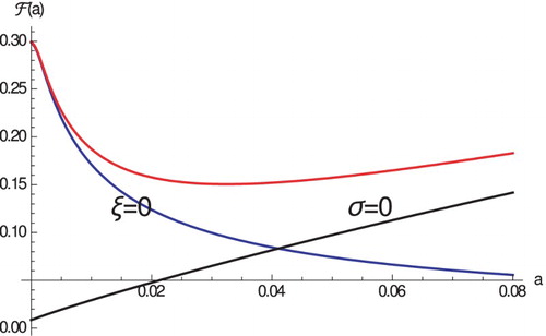
Table 2. List of Parameter Values.

Parameter	Value
$P\left(0\right)$	100
$B\left(0\right)$	1
r	1
ε	0.1
a	Variable
σ	0.001
ξ	0.001
c	Not a part of $\mathcal{F}$
d	Not a part of $\mathcal{F}$
κ	0
$m_0$	0.5

Pathogens evolve very quickly and in the process they change their reproductive rate r. The host has to adapt to the evolving pathogens. How do the case fatality proportion and the optimal immune response change with the pathogen changing reproductive rate? Figure 2 suggests that as r increases, the case fatality proportion also increases. This observation is somewhat intuitive as increasing r increases $P\left(\tau \right)$, which increases disease-induced mortality, and ultimately increases the case fatality proportion. We expect that this observation is parameter-dependent and different outcome may be possible.

Figure 2. The case fatality proportion as a function of a for three values of r. Black points denote the minimum. Parameters are given in Table 2.

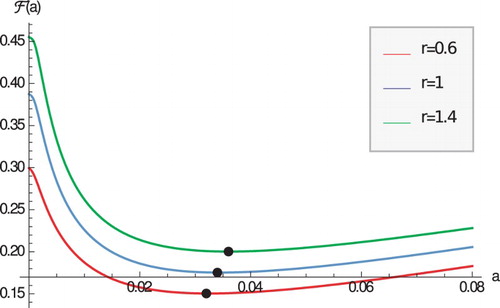
Figure 2 also suggests that as r increases, the optimal immune response rate $a^{\ast }$ also increases to compensate for the increased pathogen reproduction. This observation seems robust and was also made in the case when host lifespan in the infected class was considered as host optimization principle [17,26].

Just like maximizing the epidemiological reproduction for the pathogen is an ESS, minimizing the case fatality proportion for the host is also an ESS. ESS is a concept from adaptive dynamics which studies the evolution of the traits. Adaptive dynamics considers the long-term consequences of the potential invasion of a mutant trait, when the resident population, which adopts a resident trait, is at equilibrium. In our setting here the trait under evolution is the immune activation rate a. We will use the case fatality proportion as a proxy to the invasion fitness [10]. In the case of pathogen evolution this role is played by the reproduction number. Actually, the case fatality proportion in a sense is ‘anti-fitness’. The fitness for the host will be $1-\mathcal{F}$. Nonetheless, we will work with the case fatality proportion. We know that the case fatality proportion is function of a: $\mathcal{F}\left(a\right)$. Traits for which ${\mathcal{F}}^{\prime }\left(a\right)=0$ are called evolutionarily singular strategies. We know that the case fatality proportion can have a minimum, where the derivative vanishes. Hence, there is at least one evolutionary singular strategy. Evolutionary singular strategy can be ESS, branching point or a singular case. That can be determined graphically from a pairwise invasibility plot (PIP). PIP gives the region where the mutant using a mutant strategy $a_m$ can invade the resident, playing resident strategy $a_r$. That region is obtained from plotting the region where the inequality $\mathcal{F}\left(a_m\right)<\mathcal{F}\left(a_r\right)$ holds in the $(a_r,a_m)$ plane (see Figure 3). The evolutionarily singular strategies in a PIP are obtained from the intersection of the boundary of the invasion region with the main diagonal. Figure 3 has one evolutionarily singular strategy. 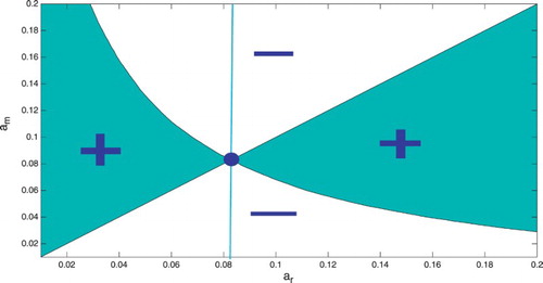This corresponds to the minimum of $\mathcal{F}\left(a\right)$ in Figure 2. The evolutionarily singular strategy is an ESS if the vertical line that passes through the singular strategy lies entirely in the region of non-invasion. That signifies that the evolutionarily singular strategy, once established, cannot be invaded by nearby mutants, that is it is an ESS. That is the case in Figure 3. Hence, minimizing the case fatality proportion is an ESS for the host.

Figure 3. Pairwise Invasibility Plot: The x-axis is the immune activation rate of the resident host. The y-axis is the immune activation rate of the mutant host. The green colour represents the region where $\mathcal{F}\left(a_m\right)<\mathcal{F}\left(a_r\right)$.

We would like to mention that although we do recognize pathogens will generally evolve faster than hosts, so that the hosts have to adapt to evolving pathogens, this aspect is not considered in building the PIP, which is based on a fixed parameter value for the pathogen. The reason for that is that in this note we are only interested in the evolution of the host as a response of an ‘evolutionary fixed’ pathogen, and not in the host–pathogen co-evolution.

One interesting observation, suggested by a referee, is that in the current immuno-epidemiological model, the ‘fitness’ of an invader host does not depend on the resident host type. In such cases, it is clear that ESS will minimize the case fatality rate, and more complex evolutionary outcomes cannot occur. Indeed, the PIP is perfectly symmetrical (if ${\mathcal{F}}_1<{\mathcal{F}}_2$, host 2 cannot invade host 1 while host 1 can invade host 2).

5. Discussion

In this paper we consider a two-host single pathogen immuno-epidemiological model. The two hosts are subjected to competitive exclusion. The main point of the paper is to show that the host that has the smallest population level case fatality proportion $\mathcal{F}$ persists, while the other dies out. Without loss of generality, we assume that host one has a smaller case fatality proportion ${\mathcal{F}}_1<{\mathcal{F}}_2$, and we consider local stability of equilibrium $E_1$. We show that if ${\mathcal{F}}_1<{\mathcal{F}}_2$, host two cannot invade host one and the stability of $E_1$ is further determined by the stability of the characteristic equation for host one in the absence of host two. We were able to establish stability of this equation in three special cases: (1) when recovery rate is zero and the derivative of the recruitment function at $N_1^{\ast }$ is nonnegative and smaller that the natural death rate; (2) when the disease-induced death rate is zero; (3) when all epidemiological parameter functions are constants and if the derivative of the recruitment function at $N_1^{\ast }$ is nonnegative, it is smaller that the natural death rate. In this case the epidemiological model turns into a system of ODEs and the condition that host one has smaller case fatality proportion takes the form $\frac{{\alpha }_1}{{\alpha }_1+{\gamma }_1+m_0}<\frac{{\alpha }_2}{{\alpha }_2+{\gamma }_2+m_0},$ where ${\alpha }_i$ is the disease-induced death rate of host i, ${\gamma }_i$ is the recovery rate and $m_0$ is the natural death rate. We surmise that in the general case the characteristic equation for host one may exhibit Hopf bifurcation and have complex roots with positive real part, leading to oscillations in the system. However, we were not able to compose an example of that case.

Returning to the immuno-epidemiological model, we consider a continuum of hosts, stratified by their immune response stimulation rate a and the case fatality proportion as a function of a, $\mathcal{F}\left(a\right)$. We argue that as a function, the case fatality proportion has a minimum because a trade-off exists between the virulence created by the pathogen and the virulence created by the immune response. From the continuum of hosts, the host that has the immune response activation rate $a^{\ast }$ that minimizes $\mathcal{F}\left(a\right)$ will outcompete the rest. We further find that if the pathogen increases its reproduction rate r, the optimal immune response rate of the host $a^{\ast }$ also increases. This is in agreement with prior results where a different principle for host evolution was used [26]. Finally, we use adaptive dynamics techniques to argue that the minimization of the case fatality proportion is an ESS for the host. Hosts that play nearby strategies cannot invade the host that plays the optimal strategy, that is the host with immune response activation rate $a^{\ast }$.

We assume logistic growth for the host as opposed to constant growth typically assumed in the literature. The reason for that is that we are looking at the evolution of the host and the host must have an option to persist and an option to die out if not fit. Constant recruitment does not give these two options; it only gives an option to persist, so evolutionary questions about the host cannot be asked in a constant recruitment model. The disease-induced mortality is assumed as a linear combination of the pathogen load and immune response. This linear combination leads to trade-off between mortality due to pathogen and mortality due to immune response and ultimately to the minimum of the CFP as explained in Section 4. Other forms, such as the one assumed by Gilchrist and Sasaki [17] will also lead to a minimum in the CFP. However, some forms of the mortality rate coupled with the form of $\beta \left(\tau \right)$ may result in monotone CFP. Gilchrist and Sasaki [17] and Pugliese [26] assume the transmission rate $\beta \left(\tau \right)$ proportional to the pathogen load. Comparison to data [22], however, suggests that the transmission rate is not linearly dependent on the pathogen load. Other forms of the transmission rate may presumably also depend on the antibody levels, although the specific form of dependence will have to be determined from experiments and data fitting. At this point we do not expect that adding dependence on the antibody levels will change significantly the results. However, transmission rates that incorporate different susceptibilities of the hosts will lead to a criterion analogous to the one derived by Bowers [9].

One interesting question that remains is whether the principle will remain if we increase the biological complexity of the model. For instance, is the principle valid in vector-host infectious disease-models or environmental transmission models? Our preliminary computations with an immuno-epidemiological vector-host model of arboviral diseases suggest that the principle remains valid [18].

In conclusion, the principle for host evolution that we derive, namely minimization of the case fatality proportion, extends prior results in [17,26] where maximization of host lifespan in the infected class was considered. Our principle is more general in the sense that it applies both to chronic diseases and to diseases with recovery.

Acknowledgments

This project may have benefitted from discussions with Hayriye Gulbudak and Vincent Cannataro. Authors also thank two referees for their helpful suggestions.

Disclosure statement

No potential conflict of interest was reported by the authors.

ORCID

Necibe Tuncer http://orcid.org/0000-0002-6388-2499

Additional information

Funding

Authors acknowledge partial support from NSF grants [DMS-1220342], [DMS-1515661] and [DMS 1515442].

References

- S. Alizon and S. Lion, Within-host parasite cooperation and the evolution of virulence, Proc. R. Soc. B 278 (2011), pp. 3738–3747. doi: 10.1098/rspb.2011.0471
- S. Alizon, F. Luciani, and R.R. Regoes, Epidemiological and clinical consequences of within-host evolution, Trends Microbiol. 19(1) (2011), pp. 24–32. doi: 10.1016/j.tim.2010.09.005
- R.M. Anderson and R.M. May, Coevolution of hosts and parasites, Parasitology 85(2) (1982), pp. 411–426. doi: 10.1017/S0031182000055360
- J. -B. André and S. Gandon, Vaccination, within-host dynamics, and virulence evolution, Evolution 60(1) (2006), pp. 13–23. doi: 10.1111/j.0014-3820.2006.tb01077.x
- C.L. Ball, M.A. Gilchrist, and D. Coombs, Modeling within-host evolution of HIV: Mutation, competition and strain replacement, Bull. Math. Biol. 69 (2007), pp. 2361–2385. doi: 10.1007/s11538-007-9223-z
- L.B. Barreiro and L. Quintana-Murci, From evolutionary genetics to human immunology: How selection shapes host defence genes, Nat. Rev. Genet. 11 (2010), pp. 17–30. doi: 10.1038/nrg2698
- S. Bonhoeffer, R.E. Lenski, and D. Ebert, The curse of the pharaoh: The evolution of virulence in pathogens with long living propagules, Proc. R. Soc. London B, Biol. Sci. 263 (1996), pp. 715–721. doi: 10.1098/rspb.1996.0107
- M. Boots and Y. Haraguchi, The evolution of costly resistance in host-parasite systems, Am. Nat. 153 (1999), pp. 359–370. doi: 10.1086/303181
- R.G. Bowers, The basic depression ratio of the host: the evolution of host resistance to microparasites, Proc. R. Soc. Lond. B 268 (2001), pp. 243–250. doi: 10.1098/rspb.2000.1360
- A. Brännström, J. Johansson, and N. von Festenberg, The hitchhiker's guide to adaptive dynamics, Games 4(3) (2013), pp. 304–328. doi: 10.3390/g4030304
- H.J. Bremermann and J. Pickering, A game-theoretical model of parasite virulence, J. Theoret. Biol. 100 (1983), pp. 411–426. doi: 10.1016/0022-5193(83)90438-1
- H.J. Bremermann and H.R. Thieme, A competitive exclusion principle for pathogen virulence, J. Math. Biol. 27 (1989), pp. 179–190. doi: 10.1007/BF00276102
- D. Claessen and A.M. de Roos, Evolution of virulence in a host–pathogen system with local pathogen transmission, Oikos 74 (1995), pp. 401–413. doi: 10.2307/3545985
- D. Coombs, M.A. Gilchrist, and C.L. Ball, Evaluating the importance of within- and between-host selection pressures on the evolution of chronic pathogens, Theor. Pop. Biol 72 (2007), pp. 576–591. doi: 10.1016/j.tpb.2007.08.005
- S. Debroy and M. Martcheva, Immuno-epidemiology and HIV/AIDS: A modeling prospective, in Mathematical Biology Research Trends, Lachlan B. Wilson, ed., Nova Publishers, New York, 2008, pp. 175–192.
- A. Giafis and R.G. Bowers, The adaptive dynamics of the evolution of host resistance to indirectly transmitted microparasites, Math. Biosci. 210 (2007), pp. 668–679. doi: 10.1016/j.mbs.2007.07.006
- M.A. Gilchrist and A. Sasaki, Modeling host-parasite coevolution: A nested approach based on mechanistic models, J. Theor. Biol. 218(3) (2002), pp. 289–308. doi: 10.1006/jtbi.2002.3076
- H. Gulbudak, V. Cannataro, N. Tuncer, and M. Martcheva, Modeling host-parasite coevolution in a coupled arbovirus within-host and between-host system, (in preparation).
- P. Lemey, A. Rambaut, and O. Pybus, HIV evolutionary dynamics within and among hosts, AIDS Rev. 8 (2006), pp. 125–140.
- M. Lipsitch and M.A. Nowak, The evolution of virulence in sexually transmitted HIV/AIDS, J. Theoret. Biol. 174 (1995), pp. 427–440. doi: 10.1006/jtbi.1995.0109
- M. Lipsitch, S. Siller, and M.A. Nowak, The evolution of virulence in pathogens with vertical and horizontal transmission, Evolution 50 (1996), pp. 1729–1741. doi: 10.2307/2410731
- M. Martcheva, An Introduction to Mathematical Epidemiology, Springer, New York, 2015.
- M. Martcheva and X. -Z. Li, Linking immunological and epidemiological dynamics of HIV: The case of super-infection, J. Biol. Dyn. 7(1) (2013), pp. 161–182. doi: 10.1080/17513758.2013.820358
- M.R. Miller, A. White, and M. Boots, The evolution of host resistance: Tolerance and control as distinct strategies, J. Theor. Biol 236 (2005), pp. 198–207. doi: 10.1016/j.jtbi.2005.03.005
- M.A. Nowak and R.M. May, Superinfection and the evolution of parasite virulence, Proc. R. Soc. London, B 255 (1994), pp. 81–89. doi: 10.1098/rspb.1994.0012
- A. Pugliese, The role of host population heterogeneity in the evolution of virulence, J. Biol. Dyn. 5 (2011), pp. 104–119. doi: 10.1080/17513758.2010.519404
- H.R. Thieme and C. Castillo-Chavez, How may infection-age-dependent infectivity affect the dynamics of HIV/AIDS?, SIAM J. Appl. Math. 53 (1993), pp. 1447–1479. doi: 10.1137/0153068
- C.A. Toft and A.J. Karter, Parasite-host coevolution, Trends Ecol. Evol. 5(10) (1990), pp. 326–329. doi: 10.1016/0169-5347(90)90179-H