Bifurcation and temporal periodic patterns in a plant–pollinator model with diffusion and time delay effects

ABSTRACT

This paper deals with a plant–pollinator model with diffusion and time delay effects. By considering the distribution of eigenvalues of the corresponding linearized equation, we first study stability of the positive constant steady-state and existence of spatially homogeneous and spatially inhomogeneous periodic solutions are investigated. We then derive an explicit formula for determining the direction and stability of the Hopf bifurcation by applying the normal form theory and the centre manifold reduction for partial functional differential equations. Finally, we present an example and numerical simulations to illustrate the obtained theoretical results.

KEYWORDS:

• Unidirectional consumer–resource interaction
• diffusion
• delay
• stability
• Hopfbifurcation

AMS SUBJECT CLASSIFICATION:

• 35K51
• 35K57
• 35B32
• 35Q92
• 37N25
• 92D25

1. Introduction

It is believed that the explosive diversification and present-day abundance of flowering plants is due to their co-evolution with animal pollinators, especially insects [13]. The interactions between flowering plants and their insect pollinators remain an important ecological relationship crucial to the maintenance of both natural and agricultural ecosystems [15]. Mathematical modeling plays a useful role in pollination research and various mathematical models have been proposed to study plant–pollinator population dynamics, see Soberon and Del Rio [24], Lundberg and Ingvarsson [19], Jang [14], Neuhauser and Fargione [20], Fishman and Hadany [8], Wang et al. [29], Wang [26], and the references cited therein.

Consumer–resource systems model some biological phenomena and relationships between consumer and resource in the real world. A resource is considered to be a biotic population that helps to maintain the population growth of its consumers, whereas a consumer exploits a resource and then reduces its growth rate. Consumer–resource systems have been extensively studied by many researchers (see Chamberlain and Holland [3], Holland and DeAngelis [11], Li et al. [17], Neuhauser and Fargione [20], Wang and DeAngelis [27], Wang et al. [28]). Bi-directional consumer–resource interactions occur when each species acts as both a consumer and a resource of the other. Uni-directional consumer–resource interactions occur when one acts as a consumer and the other as a material and/or energy resource, but neither acts as both.

Recently, Wang, DeAngelis and Holland [29] derived a plant–pollinator model based on unidirectional interactions between plants and pollinators [11]. Pollinators travel from their nest to a foraging patch, collecting food, flying back to their nests, and unloading food. Interacting with flowers individually, the pollinators remove nectar, contact pollen, and provide pollination service. Therefore, the plants provide food, seeds, nectar, and other resources for the pollinators, while the pollinators have both positive and negative effects on the plants. Let $N_1$ and $N_2$ represent the population densities of plants and pollinators, respectively. The plant–pollinator model takes the following form: (1) $\begin{array}{rl}\frac{\mathrm{d}{N}_1}{\mathrm{d}t}& =r_1{N}_1+\frac{{\alpha }_{12}{N}_1{N}_2}{1+a{N}_1+b{N}_2}-{\beta }_1{N}_1{N}_2-d_1{N}_1^2,\\ \frac{\mathrm{d}{N}_2}{\mathrm{d}t}& =\frac{{\alpha }_{21}{N}_1{N}_2}{1+a{N}_1+b{N}_2}-d_2{N}_2.\end{array}$(1) where $a,b,r_1,{\beta }_1,d_1,d_2,{\alpha }_{12},$ and ${\alpha }_{21}$ are positive constants. The parameter $r_1$ is the intrinsic growth rate of the plants and $d_1$ the self-incompatible degree. Following Fishman and Hadany [8], the positive effect of pollinators on plants is described by the Beddington–DeAngelis functional response $a{N}_1{N}_2/(1+a{N}_1+b{N}_2)$, where the parameter a is the effective equilibrium constant for (undepleted) plant–pollinator interaction, which combines traveling and unloading times spent in central place pollinator foraging, with individual-level plant–pollinator interaction. b denotes the intensity of exploitation competition among pollinators (Pianka [21]). Since a is fixed, the parameter ${\alpha }_{12}$ is regarded as the plants efficiency in translating plant–pollinator interactions into fitness (Beddington [2], DeAngelis et al. [6]) and ${\alpha }_{21}$ is the corresponding value for the pollinators. ${\beta }_1$ denotes the per-capita negative effect of pollinators on plants. $d_2$ is the per-capita mortality rate of pollinators. Wang et al. [29] studied the globally asymptotically stability of the positive equilibria and demonstrated mechanisms by which interaction outcomes of this system vary with different conditions. In particular, it was shown in [29] that system (1(1) $\begin{array}{rl}\frac{\mathrm{d}{N}_1}{\mathrm{d}t}& =r_1{N}_1+\frac{{\alpha }_{12}{N}_1{N}_2}{1+a{N}_1+b{N}_2}-{\beta }_1{N}_1{N}_2-d_1{N}_1^2,\\ \frac{\mathrm{d}{N}_2}{\mathrm{d}t}& =\frac{{\alpha }_{21}{N}_1{N}_2}{1+a{N}_1+b{N}_2}-d_2{N}_2.\end{array}$(1) ) has no periodic orbits or cycle chains in the positive quadrant.

In order to reflect the dynamical behaviours of models depending on the history, it is necessary to incorporate time delay into the models. Following Adams et al. [1], we assume that there is a time delay $\tau >0$ in the process when the pollinators translate plant–pollinator interactions into the fitness. Also, as pollinators travel between their nests and foraging patches, we further introduce the spatial diffusion with zero-flux boundary conditions. Thus, the plant–pollinator model with diffusion and time delay effects is described by the following delayed reaction–diffusion system: (2) $\begin{array}{rl}\frac{\mathrm{\partial }{N}_1(t,x)}{\mathrm{\partial }t}& =N_1(t,x)\left[r_1+\frac{{\alpha }_{12}{N}_2(t,x)}{1+a{N}_1(t,x)+b{N}_2(t,x)}-{\beta }_1{N}_2(t,x)-d_1{N}_1(t,x)\right],\\ & x\in \mathrm{\Omega },t>0,\\ \frac{\mathrm{\partial }{N}_2(t,x)}{\mathrm{\partial }t}& =D_2\mathrm{\Delta }{N}_2(t,x)+N_2(t,x)\left[\frac{{\alpha }_{21}{N}_1(t-\tau ,x)}{1+a{N}_1(t-\tau ,x)+b{N}_2(t-\tau ,x)}-d_2\right],\\ & x\in \mathrm{\Omega },t>0,\\ N_1(t,x)& =\phi (t,x)\ge 0,N_2(t,x)=\psi (t,x)\ge 0,(t,x)\in [-\tau ,0]\times \overline{\mathrm{\Omega }},\\ \frac{\mathrm{\partial }{N}_1}{\mathrm{\partial }\nu }& =\frac{\mathrm{\partial }{N}_2}{\mathrm{\partial }\nu }=0,t\ge 0,x\in \mathrm{\partial \Omega },\end{array}$(2) where $D_2>0$ denotes the diffusion coefficient of pollinators. Ω is a bounded open domain in ${\mathbb{R}}^n(n\ge 1)$ and its boundary $\mathrm{\partial \Omega }$ is smooth, $\mathrm{\Delta }={\mathrm{\partial }}^2/\mathrm{\partial }{x}_1^2+\cdots +{\mathrm{\partial }}^2/\mathrm{\partial }{x}_n^2$ is the Laplacian operator in ${\mathbb{R}}^n,$ ν is the outer normal direction on $\mathrm{\partial \Omega }$, and the homogeneous Neumann boundary conditions reflect the situation where the population cannot move across the boundary of the domain.

Throughout this paper, without of loss of generality, we consider the domain $\mathrm{\Omega }=(0,\pi )$. Thus, $\mathrm{\Delta }={\mathrm{\partial }}^2/\mathrm{\partial }{x}^2.$ We also assume that $(\phi ,\psi )\in C:=C\left(\right[-\tau ,0],X)$ and X is a suitable Hilbert space. For example, we can take $X=\left\{(N_1,N_2):N_1,N_2\in W^{2,2}(0,\pi ):\frac{\mathrm{\partial }{N}_1(t,x)}{\mathrm{\partial }x}=\frac{\mathrm{\partial }{N}_2(t,x)}{\mathrm{\partial }x}=0,x=0,\pi \right\}$ with the inner product $⟨\cdot ,\cdot ⟩$.

The rest of the paper is organized as follows. In Section 2, we consider the corresponding characteristic equation of system (2(2) $\begin{array}{rl}\frac{\mathrm{\partial }{N}_1(t,x)}{\mathrm{\partial }t}& =N_1(t,x)\left[r_1+\frac{{\alpha }_{12}{N}_2(t,x)}{1+a{N}_1(t,x)+b{N}_2(t,x)}-{\beta }_1{N}_2(t,x)-d_1{N}_1(t,x)\right],\\ & x\in \mathrm{\Omega },t>0,\\ \frac{\mathrm{\partial }{N}_2(t,x)}{\mathrm{\partial }t}& =D_2\mathrm{\Delta }{N}_2(t,x)+N_2(t,x)\left[\frac{{\alpha }_{21}{N}_1(t-\tau ,x)}{1+a{N}_1(t-\tau ,x)+b{N}_2(t-\tau ,x)}-d_2\right],\\ & x\in \mathrm{\Omega },t>0,\\ N_1(t,x)& =\phi (t,x)\ge 0,N_2(t,x)=\psi (t,x)\ge 0,(t,x)\in [-\tau ,0]\times \overline{\mathrm{\Omega }},\\ \frac{\mathrm{\partial }{N}_1}{\mathrm{\partial }\nu }& =\frac{\mathrm{\partial }{N}_2}{\mathrm{\partial }\nu }=0,t\ge 0,x\in \mathrm{\partial \Omega },\end{array}$(2) ) and give conditions on the stability of the positive constant steady-state and the existence of Hopf bifurcation. In Section 3, by applying the normal form theory and centre manifold reduction of partial functional differential equations (PFDEs) (Wu [30], Faria [7]), an explicit algorithm for determining the direction and stability of the Hopf bifurcation is given. Finally, some numerical simulations are included to support our theoretical predictions in Section 4 and a brief discussion is given in Section 5.

2. Stability and Hopf bifurcation

In this section, we consider the local stability of the positive constant steady-state and the Hopf bifurcation of system (2(2) $\begin{array}{rl}\frac{\mathrm{\partial }{N}_1(t,x)}{\mathrm{\partial }t}& =N_1(t,x)\left[r_1+\frac{{\alpha }_{12}{N}_2(t,x)}{1+a{N}_1(t,x)+b{N}_2(t,x)}-{\beta }_1{N}_2(t,x)-d_1{N}_1(t,x)\right],\\ & x\in \mathrm{\Omega },t>0,\\ \frac{\mathrm{\partial }{N}_2(t,x)}{\mathrm{\partial }t}& =D_2\mathrm{\Delta }{N}_2(t,x)+N_2(t,x)\left[\frac{{\alpha }_{21}{N}_1(t-\tau ,x)}{1+a{N}_1(t-\tau ,x)+b{N}_2(t-\tau ,x)}-d_2\right],\\ & x\in \mathrm{\Omega },t>0,\\ N_1(t,x)& =\phi (t,x)\ge 0,N_2(t,x)=\psi (t,x)\ge 0,(t,x)\in [-\tau ,0]\times \overline{\mathrm{\Omega }},\\ \frac{\mathrm{\partial }{N}_1}{\mathrm{\partial }\nu }& =\frac{\mathrm{\partial }{N}_2}{\mathrm{\partial }\nu }=0,t\ge 0,x\in \mathrm{\partial \Omega },\end{array}$(2) ) by regarding the time delay τ as the bifurcation parameter. We assume that

• (A1) ${\alpha }_{21}>a{d}_2,a_1<0,a_1^2-4a_0{a}_2=0;$

• (A2) ${\alpha }_{21}>a{d}_2,4a_0{a}_2<0.$

where $\begin{array}{rl}{a}_0& =\frac{b{\beta }_1}{{\alpha }_{21}-a{d}_2}+\frac{{\mathrm{d}}_1{d}_2{b}^2}{({\alpha }_{21}-a{d}_2{)}^2},a_1=\frac{{\beta }_1-b{r}_1}{{\alpha }_{21}-a{d}_2}+\frac{2d_1{d}_{2}b}{({\alpha }_{21}-a{d}_2{)}^2}-\frac{{\alpha }_{12}}{{\alpha }_{21}},\\ a_2& =-\frac{r_1}{{\alpha }_{21}-a{d}_2}+\frac{{\mathrm{d}}_1{d}_2}{({\alpha }_{21}-a{d}_2{)}^2}.\end{array}$

We can prove that, if (A1) or (A2) hold, then system (2(2) $\begin{array}{rl}\frac{\mathrm{\partial }{N}_1(t,x)}{\mathrm{\partial }t}& =N_1(t,x)\left[r_1+\frac{{\alpha }_{12}{N}_2(t,x)}{1+a{N}_1(t,x)+b{N}_2(t,x)}-{\beta }_1{N}_2(t,x)-d_1{N}_1(t,x)\right],\\ & x\in \mathrm{\Omega },t>0,\\ \frac{\mathrm{\partial }{N}_2(t,x)}{\mathrm{\partial }t}& =D_2\mathrm{\Delta }{N}_2(t,x)+N_2(t,x)\left[\frac{{\alpha }_{21}{N}_1(t-\tau ,x)}{1+a{N}_1(t-\tau ,x)+b{N}_2(t-\tau ,x)}-d_2\right],\\ & x\in \mathrm{\Omega },t>0,\\ N_1(t,x)& =\phi (t,x)\ge 0,N_2(t,x)=\psi (t,x)\ge 0,(t,x)\in [-\tau ,0]\times \overline{\mathrm{\Omega }},\\ \frac{\mathrm{\partial }{N}_1}{\mathrm{\partial }\nu }& =\frac{\mathrm{\partial }{N}_2}{\mathrm{\partial }\nu }=0,t\ge 0,x\in \mathrm{\partial \Omega },\end{array}$(2) ) has two boundary equilibria $E_0(0,0),$ $E_1(r_1/d_1,0),$ and a unique positive constant steady-state $E^{\ast }(N_1^{\ast },N_2^{\ast }),$ where $N_1^{\ast }=\frac{2a_0{d}_2-a_{1}b{d}_2+b{d}_2\sqrt{a_1^2-4a_0{a}_2}}{2a_0({\alpha }_{21}-a{d}_2)},N_2^{\ast }=\frac{-a_1+\sqrt{a_1^2-4a_0{a}_2}}{2a_0}.$

Let $u=N_1-N_1^{\ast },v=N_2-N_2^{\ast }.$ Then system (2(2) $\begin{array}{rl}\frac{\mathrm{\partial }{N}_1(t,x)}{\mathrm{\partial }t}& =N_1(t,x)\left[r_1+\frac{{\alpha }_{12}{N}_2(t,x)}{1+a{N}_1(t,x)+b{N}_2(t,x)}-{\beta }_1{N}_2(t,x)-d_1{N}_1(t,x)\right],\\ & x\in \mathrm{\Omega },t>0,\\ \frac{\mathrm{\partial }{N}_2(t,x)}{\mathrm{\partial }t}& =D_2\mathrm{\Delta }{N}_2(t,x)+N_2(t,x)\left[\frac{{\alpha }_{21}{N}_1(t-\tau ,x)}{1+a{N}_1(t-\tau ,x)+b{N}_2(t-\tau ,x)}-d_2\right],\\ & x\in \mathrm{\Omega },t>0,\\ N_1(t,x)& =\phi (t,x)\ge 0,N_2(t,x)=\psi (t,x)\ge 0,(t,x)\in [-\tau ,0]\times \overline{\mathrm{\Omega }},\\ \frac{\mathrm{\partial }{N}_1}{\mathrm{\partial }\nu }& =\frac{\mathrm{\partial }{N}_2}{\mathrm{\partial }\nu }=0,t\ge 0,x\in \mathrm{\partial \Omega },\end{array}$(2) ) can be rewritten as (3) $\begin{array}{r}\begin{array}{rl}\frac{\mathrm{\partial }u(t,x)}{\mathrm{\partial }t}& =(u+N_1^{\ast })\left[r_1+\frac{{\alpha }_{12}(v+N_2^{\ast })}{1+a(u+N_1^{\ast })+b(v+N_2^{\ast })}-{\beta }_1(v+N_2^{\ast })-d_1(u+N_1^{\ast })\right],\\ \frac{\mathrm{\partial }v(t,x)}{\mathrm{\partial }t}& =D_2\frac{{\mathrm{\partial }}^{2}v(t,x)}{\mathrm{\partial }{x}^2}+(v+N_2^{\ast })\left[\frac{{\alpha }_{21}\left(u\right(t-\tau ,x)+N_1^{\ast })}{1+a\left(u\right(t-\tau ,x)+N_1^{\ast })+b\left(v\right(t-\tau ,x)+N_2^{\ast })}-d_2\right],\\ \frac{\mathrm{\partial }{N}_1}{\mathrm{\partial }\nu }& =\frac{\mathrm{\partial }{N}_2}{\mathrm{\partial }\nu }=0,t\ge 0,x\in \mathrm{\partial \Omega },\\ u(t,x)& =\phi (t,x)-N_1^{\ast },v(t,x)=\psi (t,x)-N_2^{\ast },t\in [-\tau ,0],x\in \overline{\mathrm{\Omega }}.\end{array}\end{array}$(3) The positive equilibrium $E^{\ast }(N_1^{\ast },N_2^{\ast })$ of system (2(2) $\begin{array}{rl}\frac{\mathrm{\partial }{N}_1(t,x)}{\mathrm{\partial }t}& =N_1(t,x)\left[r_1+\frac{{\alpha }_{12}{N}_2(t,x)}{1+a{N}_1(t,x)+b{N}_2(t,x)}-{\beta }_1{N}_2(t,x)-d_1{N}_1(t,x)\right],\\ & x\in \mathrm{\Omega },t>0,\\ \frac{\mathrm{\partial }{N}_2(t,x)}{\mathrm{\partial }t}& =D_2\mathrm{\Delta }{N}_2(t,x)+N_2(t,x)\left[\frac{{\alpha }_{21}{N}_1(t-\tau ,x)}{1+a{N}_1(t-\tau ,x)+b{N}_2(t-\tau ,x)}-d_2\right],\\ & x\in \mathrm{\Omega },t>0,\\ N_1(t,x)& =\phi (t,x)\ge 0,N_2(t,x)=\psi (t,x)\ge 0,(t,x)\in [-\tau ,0]\times \overline{\mathrm{\Omega }},\\ \frac{\mathrm{\partial }{N}_1}{\mathrm{\partial }\nu }& =\frac{\mathrm{\partial }{N}_2}{\mathrm{\partial }\nu }=0,t\ge 0,x\in \mathrm{\partial \Omega },\end{array}$(2) ) is transformed into the zero equilibrium of system (3(3) $\begin{array}{r}\begin{array}{rl}\frac{\mathrm{\partial }u(t,x)}{\mathrm{\partial }t}& =(u+N_1^{\ast })\left[r_1+\frac{{\alpha }_{12}(v+N_2^{\ast })}{1+a(u+N_1^{\ast })+b(v+N_2^{\ast })}-{\beta }_1(v+N_2^{\ast })-d_1(u+N_1^{\ast })\right],\\ \frac{\mathrm{\partial }v(t,x)}{\mathrm{\partial }t}& =D_2\frac{{\mathrm{\partial }}^{2}v(t,x)}{\mathrm{\partial }{x}^2}+(v+N_2^{\ast })\left[\frac{{\alpha }_{21}\left(u\right(t-\tau ,x)+N_1^{\ast })}{1+a\left(u\right(t-\tau ,x)+N_1^{\ast })+b\left(v\right(t-\tau ,x)+N_2^{\ast })}-d_2\right],\\ \frac{\mathrm{\partial }{N}_1}{\mathrm{\partial }\nu }& =\frac{\mathrm{\partial }{N}_2}{\mathrm{\partial }\nu }=0,t\ge 0,x\in \mathrm{\partial \Omega },\\ u(t,x)& =\phi (t,x)-N_1^{\ast },v(t,x)=\psi (t,x)-N_2^{\ast },t\in [-\tau ,0],x\in \overline{\mathrm{\Omega }}.\end{array}\end{array}$(3) ).

Let $\begin{array}{rl}{f}^{\left(1\right)}(u,v)& =(u+N_1^{\ast })\left[r_1+\frac{{\alpha }_{12}(v+N_2^{\ast })}{1+a(u+N_1^{\ast })+b(v+N_2^{\ast })}-{\beta }_1(v+N_2^{\ast })-d_1(u+N_1^{\ast })\right],\\ f^{\left(2\right)}(u,v,w)& =(w+N_2^{\ast })\left[\frac{{\alpha }_{21}(u+N_1^{\ast })}{1+a(u+N_1^{\ast })+b(v+N_2^{\ast })}-d_2\right].\end{array}$ By the definition of the above functions, for $i,j,l\in {\mathbb{N}}_0=\{0,1,2\dots \},$ define $f_{ij}^{\left(1\right)}(i+j\ge 1)$ and $f_{ijl}^{\left(2\right)}(i+j+l\ge 1)$ as follow: $f_{ij}^{\left(1\right)}=\frac{{\mathrm{\partial }}^{i+j}{f}^{\left(1\right)}(0,0)}{\mathrm{\partial }{u}^i\mathrm{\partial }{v}^j},f_{ijl}^{\left(2\right)}=\frac{{\mathrm{\partial }}^{i+j+l}{f}^{\left(2\right)}(0,0,0)}{\mathrm{\partial }{u}^i\mathrm{\partial }{v}^j\mathrm{\partial }{w}^l},$ in particularly $\begin{array}{rl}{\alpha }_1& :=f_{10}^{\left(1\right)}=-d_1{N}_1^{\ast }-\frac{{\alpha }_{12}a{N}_1^{\ast }{N}_2^{\ast }}{(1+a{N}_1^{\ast }+b{N}_2^{\ast }{)}^2}<0,\\ {\alpha }_2& :=f_{01}^{\left(1\right)}=\frac{{\alpha }_{12}{N}_1^{\ast }(1+a{N}_1^{\ast })}{(1+a{N}_1^{\ast }+b{N}_2^{\ast }{)}^2}-{\beta }_1{N}_1^{\ast },\\ {\gamma }_1& :=f_{100}^{\left(2\right)}=\frac{{\alpha }_{21}{N}_2^{\ast }(1+b{N}_2^{\ast })}{(1+a{N}_1^{\ast }+b{N}_2^{\ast }{)}^2}>0,\\ {\gamma }_2& :=f_{010}^{\left(2\right)}=-\frac{b{\alpha }_{21}{N}_1^{\ast }{N}_2^{\ast }}{(1+a{N}_1^{\ast }+b{N}_2^{\ast }{)}^2}<0.\end{array}$ Obviously, we have ${\alpha }_1+{\gamma }_2<0.$ By Taylor expansion, Equation (3(3) $\begin{array}{r}\begin{array}{rl}\frac{\mathrm{\partial }u(t,x)}{\mathrm{\partial }t}& =(u+N_1^{\ast })\left[r_1+\frac{{\alpha }_{12}(v+N_2^{\ast })}{1+a(u+N_1^{\ast })+b(v+N_2^{\ast })}-{\beta }_1(v+N_2^{\ast })-d_1(u+N_1^{\ast })\right],\\ \frac{\mathrm{\partial }v(t,x)}{\mathrm{\partial }t}& =D_2\frac{{\mathrm{\partial }}^{2}v(t,x)}{\mathrm{\partial }{x}^2}+(v+N_2^{\ast })\left[\frac{{\alpha }_{21}\left(u\right(t-\tau ,x)+N_1^{\ast })}{1+a\left(u\right(t-\tau ,x)+N_1^{\ast })+b\left(v\right(t-\tau ,x)+N_2^{\ast })}-d_2\right],\\ \frac{\mathrm{\partial }{N}_1}{\mathrm{\partial }\nu }& =\frac{\mathrm{\partial }{N}_2}{\mathrm{\partial }\nu }=0,t\ge 0,x\in \mathrm{\partial \Omega },\\ u(t,x)& =\phi (t,x)-N_1^{\ast },v(t,x)=\psi (t,x)-N_2^{\ast },t\in [-\tau ,0],x\in \overline{\mathrm{\Omega }}.\end{array}\end{array}$(3) ) becomes (4) $\begin{array}{rl}\frac{\mathrm{\partial }u(t,x)}{\mathrm{\partial }t}& ={\alpha }_{1}u(t,x)+{\alpha }_{2}v(t,x)+\sum _{i+j\ge 2}\frac{1}{i!j!}{f}_{ij}^{\left(1\right)}{u}^i(t,x)v^j(t,x),\\ \frac{\mathrm{\partial }v(t,x)}{\mathrm{\partial }t}& =D_2\frac{{\mathrm{\partial }}^{2}v(t,x)}{\mathrm{\partial }{x}^2}+{\gamma }_{1}u(t-\tau ,x)+{\gamma }_{2}v(t-\tau ,x)\\ & +\sum _{i+j+l\ge 2}\frac{1}{i!j!l!}{f}_{ijl}^{\left(2\right)}{u}^i(t-\tau ,x)v^j(t-\tau ,x)v^l(t,x).\end{array}$(4) Let $u_1\left(t\right)=u(t,\cdot ),u_2\left(t\right)=v(t,\cdot )$ and $U=(u_1,u_2{)}^{\mathrm{T}}.$ Then system (4(4) $\begin{array}{rl}\frac{\mathrm{\partial }u(t,x)}{\mathrm{\partial }t}& ={\alpha }_{1}u(t,x)+{\alpha }_{2}v(t,x)+\sum _{i+j\ge 2}\frac{1}{i!j!}{f}_{ij}^{\left(1\right)}{u}^i(t,x)v^j(t,x),\\ \frac{\mathrm{\partial }v(t,x)}{\mathrm{\partial }t}& =D_2\frac{{\mathrm{\partial }}^{2}v(t,x)}{\mathrm{\partial }{x}^2}+{\gamma }_{1}u(t-\tau ,x)+{\gamma }_{2}v(t-\tau ,x)\\ & +\sum _{i+j+l\ge 2}\frac{1}{i!j!l!}{f}_{ijl}^{\left(2\right)}{u}^i(t-\tau ,x)v^j(t-\tau ,x)v^l(t,x).\end{array}$(4) ) can be rewritten as an abstract differential equation in the phase space $C:=C\left(\right[-\tau ,0],X),$ (5) $U^{\mathrm{\prime }}\left(t\right)=D\mathrm{\Delta }U\left(t\right)+L\left(U_t\right)+F\left(U_t\right),$(5) where $D=\left(\begin{array}{cc}0& 0\\ 0& D_2\end{array}\right),\mathrm{\Delta }=\left(\begin{array}{cc}\frac{\mathrm{\partial }}{\mathrm{\partial }{x}^2}& 0\\ 0& \frac{\mathrm{\partial }}{\mathrm{\partial }{x}^2}\end{array}\right),$ $U_t\left(\theta \right)=U(t+\theta ),-\tau \le \theta \le 0,L:C⟶X$ and $F:C⟶X$ are defined by $L\left(\varphi \right)=\left(\begin{array}{c}{\alpha }_1{\varphi }_1\left(0\right)+{\alpha }_2{\varphi }_2\left(0\right)\\ {\gamma }_1{\varphi }_1(-\tau )+{\gamma }_2{\varphi }_2(-\tau )\end{array}\right)$ and $F\left(\varphi \right)=\left(\begin{array}{c}\sum _{i+j\ge 2}\frac{1}{i!j!}{f}_{ij}^{\left(1\right)}{\varphi }_1^i\left(0\right){\varphi }_2^j\left(0\right)\\ \sum _{i+j+l\ge 2}\frac{1}{i!j!l!}{f}_{ijl}^{\left(2\right)}{\varphi }_1^i(-\tau ){\varphi }_2^j(-\tau ){\varphi }_2^l\left(0\right)\end{array}\right),$ respectively, for $\varphi =({\varphi }_1,{\varphi }_2{)}^{\mathrm{T}}\in C.$ The linearized system of system (5(5) $U^{\mathrm{\prime }}\left(t\right)=D\mathrm{\Delta }U\left(t\right)+L\left(U_t\right)+F\left(U_t\right),$(5) ) at $(0,0)$ has the form: (6) $U^{\mathrm{\prime }}\left(t\right)=D\mathrm{\Delta }U\left(t\right)+L\left(U_t\right),$(6) and its characteristic equation is (7) $\lambda y-D\mathrm{\Delta }y-L({\mathrm{e}}^{\lambda \cdot }\cdot y)=0,$(7) where $y\in \mathrm{dom}\left(\mathrm{\Delta }\right)\mathrm{\setminus }\left\{0\right\}$ and $\mathrm{dom}\left(\mathrm{\Delta }\right)\subset X.$ It is well known that the Laplacian operator Δ on X has eigenvalues $-k^2,k=0,1,2,\dots ,$ with corresponding eigenfunctions ${\beta }_k^1=\left(\genfrac{}{}{0em}{}{\cos kx}{0}\right),{\beta }_k^2=\left(\genfrac{}{}{0em}{}{0}{\cos kx}\right).$ Clearly, $({\beta }_k^1,{\beta }_k^2{)}_{k=0}^{\mathrm{\infty }}$ form a basis of X. Thus, any $y\in X$ can be expanded as Fourier series in the following form: $y=\sum _{k=0}^{\mathrm{\infty }}{Y}_k\left(\genfrac{}{}{0em}{}{{\beta }_k^1}{{\beta }_k^2}\right)\mathrm{and}{Y}_k=(⟨y,{\beta }_k^1⟩,⟨y,{\beta }_k^2⟩).$ Therefore, (7(7) $\lambda y-D\mathrm{\Delta }y-L({\mathrm{e}}^{\lambda \cdot }\cdot y)=0,$(7) ) is equivalent to $\sum _{k=0}^{\mathrm{\infty }}(⟨y,{\beta }_k^1⟩,⟨y,{\beta }_k^2⟩)\left(\begin{array}{cc}\lambda -{\alpha }_1& -{\alpha }_2\\ -{\gamma }_1{\mathrm{e}}^{-\lambda \tau }& \lambda +D_2{k}^2-{\gamma }_2{\mathrm{e}}^{-\lambda \tau }\end{array}\right)\left(\begin{array}{c}{\beta }_k^1\\ {\beta }_k^2\end{array}\right)=0,$ $k=0,1,2,\dots .$

Hence, we conclude that the characteristic equation (7(7) $\lambda y-D\mathrm{\Delta }y-L({\mathrm{e}}^{\lambda \cdot }\cdot y)=0,$(7) ) is equivalent to the following sequence of characteristic equations: (8) ${\lambda }^2+(D_2{k}^2-{\alpha }_1)\lambda -{\alpha }_1{D}_2{k}^2+(-{\gamma }_2\lambda +{\alpha }_1{\gamma }_2-{\alpha }_2{\gamma }_1){\mathrm{e}}^{-\lambda \tau }=0,k=0,1,2,\dots .$(8) Set (9) ${\mathrm{\Delta }}_k(\lambda ,\tau ):={\lambda }^2+(D_2{k}^2-{\alpha }_1)\lambda -{\alpha }_1{D}_2{k}^2+(-{\gamma }_2\lambda +{\alpha }_1{\gamma }_2-{\alpha }_2{\gamma }_1){\mathrm{e}}^{-\lambda \tau },k=0,1,2,\dots .$(9) Notice that (8(8) ${\lambda }^2+(D_2{k}^2-{\alpha }_1)\lambda -{\alpha }_1{D}_2{k}^2+(-{\gamma }_2\lambda +{\alpha }_1{\gamma }_2-{\alpha }_2{\gamma }_1){\mathrm{e}}^{-\lambda \tau }=0,k=0,1,2,\dots .$(8) ) with $\tau =0$ is the characteristic equation of the linearization of (2(2) $\begin{array}{rl}\frac{\mathrm{\partial }{N}_1(t,x)}{\mathrm{\partial }t}& =N_1(t,x)\left[r_1+\frac{{\alpha }_{12}{N}_2(t,x)}{1+a{N}_1(t,x)+b{N}_2(t,x)}-{\beta }_1{N}_2(t,x)-d_1{N}_1(t,x)\right],\\ & x\in \mathrm{\Omega },t>0,\\ \frac{\mathrm{\partial }{N}_2(t,x)}{\mathrm{\partial }t}& =D_2\mathrm{\Delta }{N}_2(t,x)+N_2(t,x)\left[\frac{{\alpha }_{21}{N}_1(t-\tau ,x)}{1+a{N}_1(t-\tau ,x)+b{N}_2(t-\tau ,x)}-d_2\right],\\ & x\in \mathrm{\Omega },t>0,\\ N_1(t,x)& =\phi (t,x)\ge 0,N_2(t,x)=\psi (t,x)\ge 0,(t,x)\in [-\tau ,0]\times \overline{\mathrm{\Omega }},\\ \frac{\mathrm{\partial }{N}_1}{\mathrm{\partial }\nu }& =\frac{\mathrm{\partial }{N}_2}{\mathrm{\partial }\nu }=0,t\ge 0,x\in \mathrm{\partial \Omega },\end{array}$(2) ) without delay at the positive equilibrium. Because $D_2{k}^2-{\alpha }_1-{\gamma }_2>0,$ so the characteristic equation (8(8) ${\lambda }^2+(D_2{k}^2-{\alpha }_1)\lambda -{\alpha }_1{D}_2{k}^2+(-{\gamma }_2\lambda +{\alpha }_1{\gamma }_2-{\alpha }_2{\gamma }_1){\mathrm{e}}^{-\lambda \tau }=0,k=0,1,2,\dots .$(8) ) with $\tau =0$ does not have a pair of purely imaginary roots for any $k\in {\mathbb{N}}_0$ with ${\mathbb{N}}_0:=\{0,1,2,\dots \}$. According to the Hopf bifurcation theorem, we obtain the following result.

Theorem 2.1.

Assume that (A1) or (A2) hold. Then system (2(2) $\begin{array}{rl}\frac{\mathrm{\partial }{N}_1(t,x)}{\mathrm{\partial }t}& =N_1(t,x)\left[r_1+\frac{{\alpha }_{12}{N}_2(t,x)}{1+a{N}_1(t,x)+b{N}_2(t,x)}-{\beta }_1{N}_2(t,x)-d_1{N}_1(t,x)\right],\\ & x\in \mathrm{\Omega },t>0,\\ \frac{\mathrm{\partial }{N}_2(t,x)}{\mathrm{\partial }t}& =D_2\mathrm{\Delta }{N}_2(t,x)+N_2(t,x)\left[\frac{{\alpha }_{21}{N}_1(t-\tau ,x)}{1+a{N}_1(t-\tau ,x)+b{N}_2(t-\tau ,x)}-d_2\right],\\ & x\in \mathrm{\Omega },t>0,\\ N_1(t,x)& =\phi (t,x)\ge 0,N_2(t,x)=\psi (t,x)\ge 0,(t,x)\in [-\tau ,0]\times \overline{\mathrm{\Omega }},\\ \frac{\mathrm{\partial }{N}_1}{\mathrm{\partial }\nu }& =\frac{\mathrm{\partial }{N}_2}{\mathrm{\partial }\nu }=0,t\ge 0,x\in \mathrm{\partial \Omega },\end{array}$(2) ) without delay cannot undergo a Hopf bifurcation at the positive constant steady-state $E^{\ast }(N_1^{\ast },N_2^{\ast })$.

Lemma 2.2.

Assume that (A1) or (A2) hold. Assume further that ${\alpha }_1{\gamma }_2-{\alpha }_2{\gamma }_1>0$. Then $\lambda =0$ is not a root of Equation (8(8) ${\lambda }^2+(D_2{k}^2-{\alpha }_1)\lambda -{\alpha }_1{D}_2{k}^2+(-{\gamma }_2\lambda +{\alpha }_1{\gamma }_2-{\alpha }_2{\gamma }_1){\mathrm{e}}^{-\lambda \tau }=0,k=0,1,2,\dots .$(8) ) for any $k\in {\mathbb{N}}_0$ with ${\mathbb{N}}_0:=\{0,1,2,\dots \}$.

Proof.

From Equation (9(9) ${\mathrm{\Delta }}_k(\lambda ,\tau ):={\lambda }^2+(D_2{k}^2-{\alpha }_1)\lambda -{\alpha }_1{D}_2{k}^2+(-{\gamma }_2\lambda +{\alpha }_1{\gamma }_2-{\alpha }_2{\gamma }_1){\mathrm{e}}^{-\lambda \tau },k=0,1,2,\dots .$(9) ), we have ${\mathrm{\Delta }}_k(0,\tau )=-{\alpha }_1{D}_2{k}^2+{\alpha }_1{\gamma }_2-{\alpha }_2{\gamma }_1.$ Since ${\alpha }_1<0,D_2>0$ and ${\alpha }_1{\gamma }_2-{\alpha }_2{\gamma }_1>0$, we obtain ${\mathrm{\Delta }}_k(0,\tau )>0$ for any $k\in {\mathbb{N}}_0,$ which implies that $\lambda =0$ is not a root of Equation (8(8) ${\lambda }^2+(D_2{k}^2-{\alpha }_1)\lambda -{\alpha }_1{D}_2{k}^2+(-{\gamma }_2\lambda +{\alpha }_1{\gamma }_2-{\alpha }_2{\gamma }_1){\mathrm{e}}^{-\lambda \tau }=0,k=0,1,2,\dots .$(8) ) for any $k\in {\mathbb{N}}_0$.

Lemma 2.3.

Assume that (A1) or (A2) hold. Assume further that ${\alpha }_1{\gamma }_2-{\alpha }_2{\gamma }_1>0.$ Then all roots of Equation (8(8) ${\lambda }^2+(D_2{k}^2-{\alpha }_1)\lambda -{\alpha }_1{D}_2{k}^2+(-{\gamma }_2\lambda +{\alpha }_1{\gamma }_2-{\alpha }_2{\gamma }_1){\mathrm{e}}^{-\lambda \tau }=0,k=0,1,2,\dots .$(8) ) with $\tau =0$ have negative real parts for all $k\in {\mathbb{N}}_0=\{0,1,2,\dots \}$ and the positive constant steady-state $E^{\ast }(N_1^{\ast },N_2^{\ast })$ of Equation (2(2) $\begin{array}{rl}\frac{\mathrm{\partial }{N}_1(t,x)}{\mathrm{\partial }t}& =N_1(t,x)\left[r_1+\frac{{\alpha }_{12}{N}_2(t,x)}{1+a{N}_1(t,x)+b{N}_2(t,x)}-{\beta }_1{N}_2(t,x)-d_1{N}_1(t,x)\right],\\ & x\in \mathrm{\Omega },t>0,\\ \frac{\mathrm{\partial }{N}_2(t,x)}{\mathrm{\partial }t}& =D_2\mathrm{\Delta }{N}_2(t,x)+N_2(t,x)\left[\frac{{\alpha }_{21}{N}_1(t-\tau ,x)}{1+a{N}_1(t-\tau ,x)+b{N}_2(t-\tau ,x)}-d_2\right],\\ & x\in \mathrm{\Omega },t>0,\\ N_1(t,x)& =\phi (t,x)\ge 0,N_2(t,x)=\psi (t,x)\ge 0,(t,x)\in [-\tau ,0]\times \overline{\mathrm{\Omega }},\\ \frac{\mathrm{\partial }{N}_1}{\mathrm{\partial }\nu }& =\frac{\mathrm{\partial }{N}_2}{\mathrm{\partial }\nu }=0,t\ge 0,x\in \mathrm{\partial \Omega },\end{array}$(2) ) with $\tau =0$ is locally asymptotically stable.

Proof.

When $\tau =0,$ Equation (9(9) ${\mathrm{\Delta }}_k(\lambda ,\tau ):={\lambda }^2+(D_2{k}^2-{\alpha }_1)\lambda -{\alpha }_1{D}_2{k}^2+(-{\gamma }_2\lambda +{\alpha }_1{\gamma }_2-{\alpha }_2{\gamma }_1){\mathrm{e}}^{-\lambda \tau },k=0,1,2,\dots .$(9) ) is equivalent to the following equation: ${\mathrm{\Delta }}_k(\lambda ,0)={\lambda }^2+(D_2{k}^2-{\alpha }_1-{\gamma }_2)\lambda -{\alpha }_1{D}_2{k}^2+{\alpha }_1{\gamma }_2-{\alpha }_2{\gamma }_1,k\in {\mathbb{N}}_0.$ Let ${\lambda }_1$ and ${\lambda }_2$ be two roots of the above equation. Then $\begin{array}{rl}{\lambda }_1+{\lambda }_2& ={\alpha }_1+{\gamma }_2-D_2{k}^2,\\ {\lambda }_1{\lambda }_2& =-{\alpha }_1{D}_2{k}^2+{\alpha }_1{\gamma }_2-{\alpha }_2{\gamma }_1.\end{array}$ Since ${\lambda }_1+{\lambda }_2<0$ and ${\lambda }_1{\lambda }_2>0,$ all roots of Equation (8(8) ${\lambda }^2+(D_2{k}^2-{\alpha }_1)\lambda -{\alpha }_1{D}_2{k}^2+(-{\gamma }_2\lambda +{\alpha }_1{\gamma }_2-{\alpha }_2{\gamma }_1){\mathrm{e}}^{-\lambda \tau }=0,k=0,1,2,\dots .$(8) ) with $\tau =0$ have negative real parts.

Let $\lambda =\mathrm{i}\omega (\omega >0)$ be a purely imaginary root of Equation (8(8) ${\lambda }^2+(D_2{k}^2-{\alpha }_1)\lambda -{\alpha }_1{D}_2{k}^2+(-{\gamma }_2\lambda +{\alpha }_1{\gamma }_2-{\alpha }_2{\gamma }_1){\mathrm{e}}^{-\lambda \tau }=0,k=0,1,2,\dots .$(8) ) for $k\in {\mathbb{N}}_0$ with ${\mathbb{N}}_0:=\{0,1,2,\dots \}.$ Then we have $-{\omega }^2+\mathrm{i}(D_2{k}^2-{\alpha }_1)\omega -{\alpha }_1{D}_2{k}^2+({\alpha }_1{\gamma }_2-{\alpha }_2{\gamma }_1){\mathrm{e}}^{-\mathrm{i}\omega \tau }-\mathrm{i}{\gamma }_2\omega {\mathrm{e}}^{-\mathrm{i}\omega \tau }=0.$ Separating the real and imaginary parts in the above equation, we obtain (10) $\begin{array}{rl}-{\omega }^2-{\alpha }_1{D}_2{k}^2& ={\gamma }_2\omega \sin \left(\omega \tau \right)-({\alpha }_1{\gamma }_2-{\alpha }_2{\gamma }_1)\cos \left(\omega \tau \right),\\ (D_2{k}^2-{\alpha }_1)\omega & =({\alpha }_1{\gamma }_2-{\alpha }_2{\gamma }_1)\sin \left(\omega \tau \right)+{\gamma }_2\omega \cos \left(\omega \tau \right),\end{array}$(10) which imply that (11) $(-{\alpha }_1{D}_2{k}^2-{\omega }^2{)}^2+(D_2{k}^2-{\alpha }_1{)}^2{\omega }^2=({\alpha }_1{\gamma }_2-{\alpha }_2{\gamma }_1{)}^2+{\gamma }_2^2{\omega }^2,$(11) i.e. (12) ${\omega }^4+(D_2^2{k}^4+{\alpha }_1^2-{\gamma }_2^2){\omega }^2+(-{\alpha }_1{D}_2{k}^2{)}^2-({\alpha }_1{\gamma }_2-{\alpha }_2{\gamma }_1{)}^2=0.$(12) Set $z={\omega }^2$, (12(12) ${\omega }^4+(D_2^2{k}^4+{\alpha }_1^2-{\gamma }_2^2){\omega }^2+(-{\alpha }_1{D}_2{k}^2{)}^2-({\alpha }_1{\gamma }_2-{\alpha }_2{\gamma }_1{)}^2=0.$(12) ) is transformed into (13) $z^2+(D_2^2{k}^4+{\alpha }_1^2-{\gamma }_2^2)z+(-{\alpha }_1{D}_2{k}^2{)}^2-({\alpha }_1{\gamma }_2-{\alpha }_2{\gamma }_1{)}^2=0.$(13) If ${\alpha }_1{D}_2{k}^2+{\alpha }_1{\gamma }_2-{\alpha }_2{\gamma }_1>0$, then Equation (13(13) $z^2+(D_2^2{k}^4+{\alpha }_1^2-{\gamma }_2^2)z+(-{\alpha }_1{D}_2{k}^2{)}^2-({\alpha }_1{\gamma }_2-{\alpha }_2{\gamma }_1{)}^2=0.$(13) ) has only one positive root which is denoted by $z_k$. Hence Equation (12(12) ${\omega }^4+(D_2^2{k}^4+{\alpha }_1^2-{\gamma }_2^2){\omega }^2+(-{\alpha }_1{D}_2{k}^2{)}^2-({\alpha }_1{\gamma }_2-{\alpha }_2{\gamma }_1{)}^2=0.$(12) ) has only one positive root $w_{+}^k=\sqrt{z_k}$. From Equation (10(10) $\begin{array}{rl}-{\omega }^2-{\alpha }_1{D}_2{k}^2& ={\gamma }_2\omega \sin \left(\omega \tau \right)-({\alpha }_1{\gamma }_2-{\alpha }_2{\gamma }_1)\cos \left(\omega \tau \right),\\ (D_2{k}^2-{\alpha }_1)\omega & =({\alpha }_1{\gamma }_2-{\alpha }_2{\gamma }_1)\sin \left(\omega \tau \right)+{\gamma }_2\omega \cos \left(\omega \tau \right),\end{array}$(10) ), we know that Equation (8(8) ${\lambda }^2+(D_2{k}^2-{\alpha }_1)\lambda -{\alpha }_1{D}_2{k}^2+(-{\gamma }_2\lambda +{\alpha }_1{\gamma }_2-{\alpha }_2{\gamma }_1){\mathrm{e}}^{-\lambda \tau }=0,k=0,1,2,\dots .$(8) ) with $k\in {\mathbb{N}}_0$ has a pair of purely imaginary roots $\pm \mathrm{i}{w}_{+}^k$ when $\tau ={\tau }_j^k,$ $j=0,1,2,\dots$, where (14) $\begin{array}{rl}(w_{+}^k{)}^2& =-\frac{D_2^2{k}^4+{\alpha }_1^2-{\gamma }_2^2}{2}\\ & +\frac{\sqrt{({\gamma }_2^2-{\alpha }_1^2-D_2^2{k}^4{)}^2-4[(-{\alpha }_1{D}_2{k}^2{)}^2-({\alpha }_1{\gamma }_2-{\alpha }_2{\gamma }_1{)}^2]}}{2},\\ {\tau }_j^k& =\left\{\begin{array}{ll}\frac{1}{w_{+}^k}(\arccos E(w_{+}^k)+2j\pi ),& \mathrm{if}F\left(w_{+}^k\right)\ge 0,\\ \frac{1}{w_{+}^k}(2\pi -\arccos E(w_{+}^k)+2j\pi ),& \mathrm{if}F\left(w_{+}^k\right)<0\end{array}\right.\end{array}$(14) with (15) $\begin{array}{rl}F\left(w_{+}^k\right)& :=\sin \left(w_{+}^k\tau \right)=\frac{-{\gamma }_2{w}_{+}^k\left(\right(w_{+}^k{)}^2+{\alpha }_1{D}_2{k}^2)+w_{+}^k(D_2{k}^2-{\alpha }_1\left)\right({\alpha }_1{\gamma }_2-{\alpha }_2{\gamma }_1)}{{\gamma }_2^2(w_{+}^k{)}^2+({\alpha }_1{\gamma }_2-{\alpha }_2{\gamma }_1{)}^2},\\ E\left(w_{+}^k\right)& :=\cos \left(w_{+}^k\tau \right)=\frac{{\alpha }_1{D}_2{k}^2({\alpha }_1{\gamma }_2-{\alpha }_2{\gamma }_1)+{\gamma }_2{D}_2(w_{+}^k{)}^2{k}^2-{\alpha }_2{\gamma }_1(w_{+}^k{)}^2}{{\gamma }_2^2(w_{+}^k{)}^2+({\alpha }_1{\gamma }_2-{\alpha }_2{\gamma }_1{)}^2}.\end{array}$(15)

Lemma 2.4.

Assume that (A1) or (A2) hold. Assume further that ${\alpha }_1{D}_2{k}^2+{\alpha }_1{\gamma }_2-{\alpha }_2{\gamma }_1>0.$ Then ${\left.\frac{\mathrm{d}{\mathrm{\Delta }}_k(\lambda ,\tau )}{\mathrm{d}\lambda }\right|}_{\lambda =\mathrm{i}{w}_{+}^k}\ne 0.$ Therefore, $\lambda =\mathrm{i}{w}_{+}^k$ is a simple root of (8(8) ${\lambda }^2+(D_2{k}^2-{\alpha }_1)\lambda -{\alpha }_1{D}_2{k}^2+(-{\gamma }_2\lambda +{\alpha }_1{\gamma }_2-{\alpha }_2{\gamma }_1){\mathrm{e}}^{-\lambda \tau }=0,k=0,1,2,\dots .$(8) ) for $k\in {\mathbb{N}}_0.$

Proof.

Firstly, we have $\begin{array}{rl}{\left.\frac{\mathrm{d}{\mathrm{\Delta }}_k(\lambda ,\tau )}{\mathrm{d}\lambda }\right|}_{\lambda =\mathrm{i}{w}_{+}^k}& =\mathrm{i}2w_{+}^k+(D_2{k}^2-{\alpha }_1)-{\gamma }_2{\mathrm{e}}^{-\mathrm{i}{w}_{+}^k{\tau }_j^k}\\ & -\left({\alpha }_1{\gamma }_2-{\alpha }_2{\gamma }_1\right){\tau }_j^k{\mathrm{e}}^{-\mathrm{i}{w}_{+}^k{\tau }_j^k}+i{\gamma }_2{w}_{+}^k{\tau }_j^k{\mathrm{e}}^{-\mathrm{i}{w}_{+}^k{\tau }_j^k}.\end{array}$ Then, from ${\mathrm{\Delta }}_k(\lambda ,\tau )=0,$ we obtain that $\begin{array}{rl}& [2\lambda +(D_2{k}^2-{\alpha }_1)-{\gamma }_2{\mathrm{e}}^{-\lambda \tau }-\tau ({\alpha }_1{\gamma }_2-{\alpha }_2{\gamma }_1-{\gamma }_2\lambda \left){\mathrm{e}}^{-\lambda \tau }\right]\frac{\mathrm{d}\lambda \left(\tau \right)}{\mathrm{d}\tau }\\ & =\lambda ({\alpha }_1{\gamma }_2-{\alpha }_2{\gamma }_1-{\gamma }_2\lambda ){\mathrm{e}}^{-\lambda \tau }.\end{array}$ Thus, if $\mathrm{d}{\mathrm{\Delta }}_k(\lambda ,\tau )/\mathrm{d}\lambda {|}_{\lambda =\mathrm{i}{w}_{+}^k}=0,$ then $\mathrm{i}{w}_{+}^k({\alpha }_1{\gamma }_2-{\alpha }_2{\gamma }_1-{\gamma }_2\mathrm{i}{w}_{+}^k){\mathrm{e}}^{-\mathrm{i}{w}_{+}^k{\tau }_j^k}=0.$ Since $w_{+}^k>0,$ we have ${\alpha }_1{\gamma }_2-{\alpha }_2{\gamma }_1-{\gamma }_2\mathrm{i}{w}_{+}^k=0$ which implies that ${\alpha }_1{\gamma }_2-{\alpha }_2{\gamma }_1=-{\gamma }_2=0.$ However, $-{\gamma }_2>0.$ Hence, we have ${\left.\frac{\mathrm{d}{\mathrm{\Delta }}_k(\lambda ,\tau )}{\mathrm{d}\lambda }\right|}_{\lambda =\mathrm{i}{w}_{+}^k}\ne 0.$ This completes the proof.

Lemma 2.5.

Assume that (A1) or (A2) hold. Assume further that ${\alpha }_1{D}_2{k}^2+{\alpha }_1{\gamma }_2-{\alpha }_2{\gamma }_1>0.$ Let $\lambda \left(\tau \right)=\mu \left(\tau \right)+\mathrm{i}w\left(\tau \right)$ be the root of Equation (8(8) ${\lambda }^2+(D_2{k}^2-{\alpha }_1)\lambda -{\alpha }_1{D}_2{k}^2+(-{\gamma }_2\lambda +{\alpha }_1{\gamma }_2-{\alpha }_2{\gamma }_1){\mathrm{e}}^{-\lambda \tau }=0,k=0,1,2,\dots .$(8) ) for $k\in {\mathbb{N}}_0$ satisfying $\mu \left({\tau }_j^k\right)=0,w\left({\tau }_j^k\right)=w_{+}^k,$ $j\in {\mathbb{N}}_0.$ Then $\lambda \left(\tau \right)$ satisfies the following transversality condition: $\mathrm{sign}{\left\{\mathrm{Re}\left(\frac{\mathrm{d}\lambda }{\mathrm{d}\tau }\right)\right\}}_{\tau ={\tau }_j^k}>0.$

Proof.

Differentiating both sides of Equation (8(8) ${\lambda }^2+(D_2{k}^2-{\alpha }_1)\lambda -{\alpha }_1{D}_2{k}^2+(-{\gamma }_2\lambda +{\alpha }_1{\gamma }_2-{\alpha }_2{\gamma }_1){\mathrm{e}}^{-\lambda \tau }=0,k=0,1,2,\dots .$(8) ) with respect to τ yields ${\left(\frac{\mathrm{d}\lambda }{\mathrm{d}\tau }\right)}^{-1}=\frac{2\lambda {\mathrm{e}}^{\lambda \tau }-({\alpha }_1-D_2{k}^2){\mathrm{e}}^{\lambda \tau }-{\gamma }_2}{({\alpha }_1{\gamma }_2-{\alpha }_2{\gamma }_1)\lambda -{\gamma }_2{\lambda }^2}-\frac{\tau }{\lambda }.$ From Equation (10(10) $\begin{array}{rl}-{\omega }^2-{\alpha }_1{D}_2{k}^2& ={\gamma }_2\omega \sin \left(\omega \tau \right)-({\alpha }_1{\gamma }_2-{\alpha }_2{\gamma }_1)\cos \left(\omega \tau \right),\\ (D_2{k}^2-{\alpha }_1)\omega & =({\alpha }_1{\gamma }_2-{\alpha }_2{\gamma }_1)\sin \left(\omega \tau \right)+{\gamma }_2\omega \cos \left(\omega \tau \right),\end{array}$(10) ), we have $\begin{array}{rl}\mathrm{sign}{\left\{\mathrm{Re}{\left(\frac{\mathrm{d}\lambda }{\mathrm{d}\tau }\right)}^{-1}\right\}}_{\tau ={\tau }_j^k}& =\mathrm{sign}\mathrm{Re}{\left(\frac{2\lambda {\mathrm{e}}^{\lambda \tau }-({\alpha }_1-D_2{k}^2){\mathrm{e}}^{\lambda \tau }-{\gamma }_2}{({\alpha }_1{\gamma }_2-{\alpha }_2{\gamma }_1)\lambda -{\gamma }_2{\lambda }^2}-\frac{\tau }{\lambda }\right)}_{\tau ={\tau }_j^k}\\ & =\mathrm{sign}\left[\frac{2(w_{+}^k{)}^2-{\gamma }_2^2+({\alpha }_1-D_2{k}^2{)}^2+2{\alpha }_1{D}_2{k}^2}{({\alpha }_1{\gamma }_2-{\alpha }_2{\gamma }_1{)}^2+{\gamma }_2^2(w_{+}^k{)}^2}\right].\end{array}$ By inserting the expression of $(w_{+}^k{)}^2$ into the last expression, we obtain that $\mathrm{sign}{\left\{\mathrm{Re}{\left(\frac{\mathrm{d}\lambda }{\mathrm{d}\tau }\right)}^{-1}\right\}}_{\tau ={\tau }_j^k}>0.$ The proof is complete.

Notice that Equation (8(8) ${\lambda }^2+(D_2{k}^2-{\alpha }_1)\lambda -{\alpha }_1{D}_2{k}^2+(-{\gamma }_2\lambda +{\alpha }_1{\gamma }_2-{\alpha }_2{\gamma }_1){\mathrm{e}}^{-\lambda \tau }=0,k=0,1,2,\dots .$(8) ) with k=0 is the characteristic equation of the linearization of (2(2) $\begin{array}{rl}\frac{\mathrm{\partial }{N}_1(t,x)}{\mathrm{\partial }t}& =N_1(t,x)\left[r_1+\frac{{\alpha }_{12}{N}_2(t,x)}{1+a{N}_1(t,x)+b{N}_2(t,x)}-{\beta }_1{N}_2(t,x)-d_1{N}_1(t,x)\right],\\ & x\in \mathrm{\Omega },t>0,\\ \frac{\mathrm{\partial }{N}_2(t,x)}{\mathrm{\partial }t}& =D_2\mathrm{\Delta }{N}_2(t,x)+N_2(t,x)\left[\frac{{\alpha }_{21}{N}_1(t-\tau ,x)}{1+a{N}_1(t-\tau ,x)+b{N}_2(t-\tau ,x)}-d_2\right],\\ & x\in \mathrm{\Omega },t>0,\\ N_1(t,x)& =\phi (t,x)\ge 0,N_2(t,x)=\psi (t,x)\ge 0,(t,x)\in [-\tau ,0]\times \overline{\mathrm{\Omega }},\\ \frac{\mathrm{\partial }{N}_1}{\mathrm{\partial }\nu }& =\frac{\mathrm{\partial }{N}_2}{\mathrm{\partial }\nu }=0,t\ge 0,x\in \mathrm{\partial \Omega },\end{array}$(2) ) without diffusion at the positive equilibrium. By Rouché theorem and Lemmas 5(5) $U^{\mathrm{\prime }}\left(t\right)=D\mathrm{\Delta }U\left(t\right)+L\left(U_t\right)+F\left(U_t\right),$(5) – 7(7) $\lambda y-D\mathrm{\Delta }y-L({\mathrm{e}}^{\lambda \cdot }\cdot y)=0,$(7) , we have the following results [22,23] :

Theorem 2.6.

Assume that (A1) or (A2) hold. Assume further that ${\alpha }_1{\gamma }_2-{\alpha }_2{\gamma }_1>0.$ The following statements hold:

1. If $\tau \in [0,{\tau }_0^0),$ then all roots of Equation (8(8) ${\lambda }^2+(D_2{k}^2-{\alpha }_1)\lambda -{\alpha }_1{D}_2{k}^2+(-{\gamma }_2\lambda +{\alpha }_1{\gamma }_2-{\alpha }_2{\gamma }_1){\mathrm{e}}^{-\lambda \tau }=0,k=0,1,2,\dots .$(8) ) with k=0 have negative real parts;

2. If $\tau >{\tau }_0^0,$ then system (8(8) ${\lambda }^2+(D_2{k}^2-{\alpha }_1)\lambda -{\alpha }_1{D}_2{k}^2+(-{\gamma }_2\lambda +{\alpha }_1{\gamma }_2-{\alpha }_2{\gamma }_1){\mathrm{e}}^{-\lambda \tau }=0,k=0,1,2,\dots .$(8) ) with k=0 has at least one root with positive real part;

3. If $\tau ={\tau }_0^0,$ then system (8(8) ${\lambda }^2+(D_2{k}^2-{\alpha }_1)\lambda -{\alpha }_1{D}_2{k}^2+(-{\gamma }_2\lambda +{\alpha }_1{\gamma }_2-{\alpha }_2{\gamma }_1){\mathrm{e}}^{-\lambda \tau }=0,k=0,1,2,\dots .$(8) ) with k=0 has a pair of simple purely imaginary roots $\pm \mathrm{i}{w}_{+}^0,$ and all roots of (8(8) ${\lambda }^2+(D_2{k}^2-{\alpha }_1)\lambda -{\alpha }_1{D}_2{k}^2+(-{\gamma }_2\lambda +{\alpha }_1{\gamma }_2-{\alpha }_2{\gamma }_1){\mathrm{e}}^{-\lambda \tau }=0,k=0,1,2,\dots .$(8) ) with $k=0,$ except $\pm \mathrm{i}{w}_{+}^0,$ have negative real parts.

Furthermore, we can obtain the following results:

Theorem 2.7.

Assume that (A1) or (A2) hold. Assume further that ${\alpha }_1{\gamma }_2-{\alpha }_2{\gamma }_1>0,$ ${\alpha }_1(D_2+{\gamma }_2)-{\alpha }_2{\gamma }_1<0$ and $D_2^2+{\alpha }_1^2-{\gamma }_2^2>0.$ Then Equation (8(8) ${\lambda }^2+(D_2{k}^2-{\alpha }_1)\lambda -{\alpha }_1{D}_2{k}^2+(-{\gamma }_2\lambda +{\alpha }_1{\gamma }_2-{\alpha }_2{\gamma }_1){\mathrm{e}}^{-\lambda \tau }=0,k=0,1,2,\dots .$(8) ) with $\tau ={\tau }_j^0(j=0,1,2,\dots )$ has a pair of simple purely imaginary roots $\pm \mathrm{i}{w}_{+}^0,$ and all roots of Equation (8(8) ${\lambda }^2+(D_2{k}^2-{\alpha }_1)\lambda -{\alpha }_1{D}_2{k}^2+(-{\gamma }_2\lambda +{\alpha }_1{\gamma }_2-{\alpha }_2{\gamma }_1){\mathrm{e}}^{-\lambda \tau }=0,k=0,1,2,\dots .$(8) ) for any $k\in {\mathbb{N}}_0,$ except $\pm \mathrm{i}{w}_{+}^0,$ have no zero real parts. Moreover, for $\tau ={\tau }_0^0,$ all roots of Equation (8(8) ${\lambda }^2+(D_2{k}^2-{\alpha }_1)\lambda -{\alpha }_1{D}_2{k}^2+(-{\gamma }_2\lambda +{\alpha }_1{\gamma }_2-{\alpha }_2{\gamma }_1){\mathrm{e}}^{-\lambda \tau }=0,k=0,1,2,\dots .$(8) ) for any $k\in {\mathbb{N}}_0,$ except $\pm \mathrm{i}{w}_{+}^0,$ have negative real parts.

Theorem 2.8.

Assume that (A1) or (A2) hold. Assume further that ${\alpha }_1{\gamma }_2-{\alpha }_2{\gamma }_1>0,$ ${\alpha }_1(D_2+{\gamma }_2)-{\alpha }_2{\gamma }_1<0$ and $D_2^2+{\alpha }_1^2-{\gamma }_2^2>0.$ The following statements hold:

1. If $\tau \in [0,{\tau }_0^0),$ then the positive constant steady-state $E^{\ast }(N_1^{\ast },N_2^{\ast })$ is asymptotically stable;

2. If $\tau >{\tau }_0^0,$ then the positive constant steady-state $E^{\ast }(N_1^{\ast },N_2^{\ast })$ is unstable;

3. $\tau ={\tau }_j^0(j=0,1,2,\dots )$ are Hopf bifurcation values of system (2(2) $\begin{array}{rl}\frac{\mathrm{\partial }{N}_1(t,x)}{\mathrm{\partial }t}& =N_1(t,x)\left[r_1+\frac{{\alpha }_{12}{N}_2(t,x)}{1+a{N}_1(t,x)+b{N}_2(t,x)}-{\beta }_1{N}_2(t,x)-d_1{N}_1(t,x)\right],\\ & x\in \mathrm{\Omega },t>0,\\ \frac{\mathrm{\partial }{N}_2(t,x)}{\mathrm{\partial }t}& =D_2\mathrm{\Delta }{N}_2(t,x)+N_2(t,x)\left[\frac{{\alpha }_{21}{N}_1(t-\tau ,x)}{1+a{N}_1(t-\tau ,x)+b{N}_2(t-\tau ,x)}-d_2\right],\\ & x\in \mathrm{\Omega },t>0,\\ N_1(t,x)& =\phi (t,x)\ge 0,N_2(t,x)=\psi (t,x)\ge 0,(t,x)\in [-\tau ,0]\times \overline{\mathrm{\Omega }},\\ \frac{\mathrm{\partial }{N}_1}{\mathrm{\partial }\nu }& =\frac{\mathrm{\partial }{N}_2}{\mathrm{\partial }\nu }=0,t\ge 0,x\in \mathrm{\partial \Omega },\end{array}$(2) ) and these Hopf bifurcations are all spatially homogeneous.

Denote $\tilde{N}=\sqrt{\frac{|{\alpha }_1{\gamma }_2-{\alpha }_2{\gamma }_1|}{-{\alpha }_1{D}_2}}\mathrm{and}{N}_1=\left\{\begin{array}{ll}\tilde{N}-1,& \tilde{N}\in \mathbb{N}.\\ \left[\tilde{N}\right],& \tilde{N}\notin \mathbb{N}.\end{array}\right.$

From Equation (14(14) $\begin{array}{rl}(w_{+}^k{)}^2& =-\frac{D_2^2{k}^4+{\alpha }_1^2-{\gamma }_2^2}{2}\\ & +\frac{\sqrt{({\gamma }_2^2-{\alpha }_1^2-D_2^2{k}^4{)}^2-4[(-{\alpha }_1{D}_2{k}^2{)}^2-({\alpha }_1{\gamma }_2-{\alpha }_2{\gamma }_1{)}^2]}}{2},\\ {\tau }_j^k& =\left\{\begin{array}{ll}\frac{1}{w_{+}^k}(\arccos E(w_{+}^k)+2j\pi ),& \mathrm{if}F\left(w_{+}^k\right)\ge 0,\\ \frac{1}{w_{+}^k}(2\pi -\arccos E(w_{+}^k)+2j\pi ),& \mathrm{if}F\left(w_{+}^k\right)<0\end{array}\right.\end{array}$(14) ), we have ${\tau }_j^k<{\tau }_{j+1}^k$ for any $0\le k\le N_1,j\in {\mathbb{N}}_0.$ In the rest of this paper, we assume that $F\left(w_{+}^k\right)\ge 0$ and have the following lemma. The case for $F\left(w_{+}^k\right)<0$ can be discussed in a similar way.

Lemma 2.9.

Let ${\tau }_j^k$ be defined as Equation (14(14) $\begin{array}{rl}(w_{+}^k{)}^2& =-\frac{D_2^2{k}^4+{\alpha }_1^2-{\gamma }_2^2}{2}\\ & +\frac{\sqrt{({\gamma }_2^2-{\alpha }_1^2-D_2^2{k}^4{)}^2-4[(-{\alpha }_1{D}_2{k}^2{)}^2-({\alpha }_1{\gamma }_2-{\alpha }_2{\gamma }_1{)}^2]}}{2},\\ {\tau }_j^k& =\left\{\begin{array}{ll}\frac{1}{w_{+}^k}(\arccos E(w_{+}^k)+2j\pi ),& \mathrm{if}F\left(w_{+}^k\right)\ge 0,\\ \frac{1}{w_{+}^k}(2\pi -\arccos E(w_{+}^k)+2j\pi ),& \mathrm{if}F\left(w_{+}^k\right)<0\end{array}\right.\end{array}$(14) ). Assume that (A1) or (A2) hold. Assume further that ${\alpha }_1{D}_2{N}_1^2+{\alpha }_1{\gamma }_2-{\alpha }_2{\gamma }_1>0,{\alpha }_1<{\gamma }_2,{\gamma }_2{D}_2{N}_1^2-{\alpha }_2{\gamma }_1>0$ and ${\alpha }_1{D}_2({\alpha }_1{\gamma }_2-{\alpha }_2{\gamma }_1)+{\gamma }_2{D}_2(w_{+}^1{)}^2-{\alpha }_2{\gamma }_1(w_{+}^1{)}^2<0.$ Then for any $1\le k\le N_1,j\in {\mathbb{N}}_0,$ ${\tau }_j^k<{\tau }_j^{k+1}.$

Proof.

From Equation (12(12) ${\omega }^4+(D_2^2{k}^4+{\alpha }_1^2-{\gamma }_2^2){\omega }^2+(-{\alpha }_1{D}_2{k}^2{)}^2-({\alpha }_1{\gamma }_2-{\alpha }_2{\gamma }_1{)}^2=0.$(12) ), we have $(w_{+}^k{)}^2=\frac{2}{\sqrt{Y_k^2+\frac{4}{W_k}}+Y_k},$ where $\begin{array}{rl}{Y}_k& =\frac{D_2^2{k}^4+{\alpha }_1^2-{\gamma }_2^2}{({\alpha }_1{\gamma }_2-{\alpha }_2{\gamma }_1{)}^2-(-{\alpha }_1{D}_2{k}^2{)}^2},\\ W_k& =({\alpha }_1{\gamma }_2-{\alpha }_2{\gamma }_1{)}^2-(-{\alpha }_1{D}_2{k}^2{)}^2.\end{array}$ Simple computation shows that $\begin{array}{rl}\frac{\mathrm{d}{w}_{+}^k}{\mathrm{d}{Y}_k}& =\frac{-(1+Y_k╱\sqrt{Y_k^2+4╱W_k})}{\sqrt{2}(\sqrt{Y_k^2+4╱W_k}+Y_k{)}^{3/2}}<0,\\ \frac{\mathrm{d}{Y}_k}{\mathrm{d}k}& =\frac{4D_2^2{k}^3\left[\right({\alpha }_1{\gamma }_2-{\alpha }_2{\gamma }_1{)}^2+{\alpha }_1^2({\alpha }_1^2-{\gamma }_2^2)]}{\left[\right({\alpha }_1{\gamma }_2-{\alpha }_2{\gamma }_1{)}^2-({\alpha }_1{D}_2{k}^2{)}^2{]}^2}>0.\end{array}$ Notice that $W_k$ is strictly decreasing in k for $0\le k\le N_1.$ Then we obtain that $w_{+}^k$ is strictly decreasing in k for $0\le k\le N_1.$ From Equation (15(15) $\begin{array}{rl}F\left(w_{+}^k\right)& :=\sin \left(w_{+}^k\tau \right)=\frac{-{\gamma }_2{w}_{+}^k\left(\right(w_{+}^k{)}^2+{\alpha }_1{D}_2{k}^2)+w_{+}^k(D_2{k}^2-{\alpha }_1\left)\right({\alpha }_1{\gamma }_2-{\alpha }_2{\gamma }_1)}{{\gamma }_2^2(w_{+}^k{)}^2+({\alpha }_1{\gamma }_2-{\alpha }_2{\gamma }_1{)}^2},\\ E\left(w_{+}^k\right)& :=\cos \left(w_{+}^k\tau \right)=\frac{{\alpha }_1{D}_2{k}^2({\alpha }_1{\gamma }_2-{\alpha }_2{\gamma }_1)+{\gamma }_2{D}_2(w_{+}^k{)}^2{k}^2-{\alpha }_2{\gamma }_1(w_{+}^k{)}^2}{{\gamma }_2^2(w_{+}^k{)}^2+({\alpha }_1{\gamma }_2-{\alpha }_2{\gamma }_1{)}^2}.\end{array}$(15) ), we have $E\left(w_{+}^k\right)=\frac{{\alpha }_1{D}_2{k}^2({\alpha }_1{\gamma }_2-{\alpha }_2{\gamma }_1)+{\gamma }_2{D}_2(w_{+}^k{)}^2{k}^2-{\alpha }_2{\gamma }_1(w_{+}^k{)}^2}{{\gamma }_2^2(w_{+}^k{)}^2+({\alpha }_1{\gamma }_2-{\alpha }_2{\gamma }_1{)}^2}.$ By direct computation, we have $\begin{array}{rl}\frac{\mathrm{d}E\left(w_{+}^k\right)}{\mathrm{d}k}& =\frac{\left[2{\alpha }_1{D}_{2}k\right({\alpha }_1{\gamma }_2-{\alpha }_2{\gamma }_1)+2k{\gamma }_2{D}_2(w_{+}^k{)}^2\left]\right[{\gamma }_2^2(w_{+}^k{)}^2+({\alpha }_1{\gamma }_2-{\alpha }_2{\gamma }_1{)}^2]}{\left[{\gamma }_2^2\right(w_{+}^k{)}^2+({\alpha }_1{\gamma }_2-{\alpha }_2{\gamma }_1{)}^2{]}^2}\\ & +\frac{\left[2{\gamma }_2{D}_2{k}^2{w}_{+}^k\left(\frac{\mathrm{d}{w}_{+}^k}{\mathrm{d}k}\right)-2{\alpha }_2{\gamma }_1{w}_{+}^k\left(\frac{\mathrm{d}{w}_{+}^k}{\mathrm{d}k}\right)\right]\left[{\gamma }_2^2\right(w_{+}^k{)}^2+({\alpha }_1{\gamma }_2-{\alpha }_2{\gamma }_1{)}^2]}{\left[{\gamma }_2^2\right(w_{+}^k{)}^2+({\alpha }_1{\gamma }_2-{\alpha }_2{\gamma }_1{)}^2{]}^2}\\ & -\frac{2{\gamma }_2^2{w}_{+}^k\left(\frac{\mathrm{d}{w}_{+}^k}{\mathrm{d}k}\right)\left[{\alpha }_1{D}_2{k}^2\right({\alpha }_1{\gamma }_2-{\alpha }_2{\gamma }_1)+{\gamma }_2{D}_2(w_{+}^k{)}^2{k}^2-{\alpha }_2{\gamma }_1\left(w_{+}^k{)}^2\right]}{\left[{\gamma }_2^2\right(w_{+}^k{)}^2+({\alpha }_1{\gamma }_2-{\alpha }_2{\gamma }_1{)}^2{]}^2}.\end{array}$ Since $d{w}_{+}^k╱dk<0,$ by the fact that ${\alpha }_1{D}_2({\alpha }_1{\gamma }_2-{\alpha }_2{\gamma }_1)+{\gamma }_2{D}_2(w_{+}^1{)}^2-{\alpha }_2{\gamma }_1(w_{+}^1{)}^2<0$ and ${\gamma }_2{D}_2{N}_1^2-{\alpha }_2{\gamma }_1>0$, we obtain $dE\left(w_{+}^k\right)╱dk<0.$ That is, $E\left(w_{+}^k\right)$ is strictly decreasing in k for $1\le k\le N_1.$ So $\arccos \left(E\right(w_{+}^k\left)\right)$ is strictly increasing in k for $1\le k\le N_1.$ From Equation (14(14) $\begin{array}{rl}(w_{+}^k{)}^2& =-\frac{D_2^2{k}^4+{\alpha }_1^2-{\gamma }_2^2}{2}\\ & +\frac{\sqrt{({\gamma }_2^2-{\alpha }_1^2-D_2^2{k}^4{)}^2-4[(-{\alpha }_1{D}_2{k}^2{)}^2-({\alpha }_1{\gamma }_2-{\alpha }_2{\gamma }_1{)}^2]}}{2},\\ {\tau }_j^k& =\left\{\begin{array}{ll}\frac{1}{w_{+}^k}(\arccos E(w_{+}^k)+2j\pi ),& \mathrm{if}F\left(w_{+}^k\right)\ge 0,\\ \frac{1}{w_{+}^k}(2\pi -\arccos E(w_{+}^k)+2j\pi ),& \mathrm{if}F\left(w_{+}^k\right)<0\end{array}\right.\end{array}$(14) ), if $F\left(w_{+}^k\right)\ge 0,$ then ${\tau }_j^k$ is strictly increasing in k for $1\le k\le N_1$.

From the above lemma, we have ${\tau }_0^k<{\tau }_1^k<{\tau }_2^k<\cdots <{\tau }_j^k<\cdots$ for any $0\le k\le N_1$ and ${\tau }_j^1<{\tau }_j^2<{\tau }_j^3<\cdots <{\tau }_j^n<\cdots <{\tau }_j^{N_1},j\in {\mathbb{N}}_0.$ Denote $\begin{array}{rl}\mathcal{F}& :=\{{\tau }_j^k:{\tau }_j^k\ne {\tau }_m^n,{\tau }_j^k\ne {\tau }_l^0,1\le n<k\le N_1,j<m\mathrm{or}1\le k<n\le N_1,\\ j& >m,j,m,l\in {\mathbb{N}}_0\}.\end{array}$

From the above analysis, we have the following conclusion.

Theorem 2.10.

Assume that (A1) or (A2) hold. Assume further that ${\alpha }_1{D}_2{N}_1^2+{\alpha }_1{\gamma }_2-{\alpha }_2{\gamma }_1>0,{\alpha }_1<{\gamma }_2,{\gamma }_2{D}_2{N}_1^2-{\alpha }_2{\gamma }_1>0$ and ${\alpha }_1{D}_2({\alpha }_1{\gamma }_2-{\alpha }_2{\gamma }_1)+{\gamma }_2{D}_2(w_{+}^1{)}^2-{\alpha }_2{\gamma }_1(w_{+}^1{)}^2<0.$ The following statements are true:

1. If $\tau \in [0,min\{{\tau }_0^0,{\tau }_0^1\left\}\right),$ then the positive constant steady-state $E^{\ast }(N_1^{\ast },N_2^{\ast })$ is asymptotically stable;

2. If $\tau >min\{{\tau }_0^0,{\tau }_0^1\},$ then the positive constant steady-state $E^{\ast }(N_1^{\ast },N_2^{\ast })$ is unstable;

3. $\tau \in \mathcal{F}$ is a Hopf bifurcation value of system (2(2) $\begin{array}{rl}\frac{\mathrm{\partial }{N}_1(t,x)}{\mathrm{\partial }t}& =N_1(t,x)\left[r_1+\frac{{\alpha }_{12}{N}_2(t,x)}{1+a{N}_1(t,x)+b{N}_2(t,x)}-{\beta }_1{N}_2(t,x)-d_1{N}_1(t,x)\right],\\ & x\in \mathrm{\Omega },t>0,\\ \frac{\mathrm{\partial }{N}_2(t,x)}{\mathrm{\partial }t}& =D_2\mathrm{\Delta }{N}_2(t,x)+N_2(t,x)\left[\frac{{\alpha }_{21}{N}_1(t-\tau ,x)}{1+a{N}_1(t-\tau ,x)+b{N}_2(t-\tau ,x)}-d_2\right],\\ & x\in \mathrm{\Omega },t>0,\\ N_1(t,x)& =\phi (t,x)\ge 0,N_2(t,x)=\psi (t,x)\ge 0,(t,x)\in [-\tau ,0]\times \overline{\mathrm{\Omega }},\\ \frac{\mathrm{\partial }{N}_1}{\mathrm{\partial }\nu }& =\frac{\mathrm{\partial }{N}_2}{\mathrm{\partial }\nu }=0,t\ge 0,x\in \mathrm{\partial \Omega },\end{array}$(2) ) and these Hopf bifurcations are all spatially inhomogeneous.

3. Properties of Hopf bifurcations

In this section, we shall study the direction, stability and the period of bifurcating periodic solution by applying the normal form theory and the centre manifold theorem presented in [7,10,30]. Let ${\tau }_j^k\in \mathcal{F}\cup \{{\tau }_j^0,j\in {\mathbb{N}}_0\}.$ Normalizing the delay τ in system (4(4) $\begin{array}{rl}\frac{\mathrm{\partial }u(t,x)}{\mathrm{\partial }t}& ={\alpha }_{1}u(t,x)+{\alpha }_{2}v(t,x)+\sum _{i+j\ge 2}\frac{1}{i!j!}{f}_{ij}^{\left(1\right)}{u}^i(t,x)v^j(t,x),\\ \frac{\mathrm{\partial }v(t,x)}{\mathrm{\partial }t}& =D_2\frac{{\mathrm{\partial }}^{2}v(t,x)}{\mathrm{\partial }{x}^2}+{\gamma }_{1}u(t-\tau ,x)+{\gamma }_{2}v(t-\tau ,x)\\ & +\sum _{i+j+l\ge 2}\frac{1}{i!j!l!}{f}_{ijl}^{\left(2\right)}{u}^i(t-\tau ,x)v^j(t-\tau ,x)v^l(t,x).\end{array}$(4) ) by the time-scaling $t\to t/\tau$, Equation (4(4) $\begin{array}{rl}\frac{\mathrm{\partial }u(t,x)}{\mathrm{\partial }t}& ={\alpha }_{1}u(t,x)+{\alpha }_{2}v(t,x)+\sum _{i+j\ge 2}\frac{1}{i!j!}{f}_{ij}^{\left(1\right)}{u}^i(t,x)v^j(t,x),\\ \frac{\mathrm{\partial }v(t,x)}{\mathrm{\partial }t}& =D_2\frac{{\mathrm{\partial }}^{2}v(t,x)}{\mathrm{\partial }{x}^2}+{\gamma }_{1}u(t-\tau ,x)+{\gamma }_{2}v(t-\tau ,x)\\ & +\sum _{i+j+l\ge 2}\frac{1}{i!j!l!}{f}_{ijl}^{\left(2\right)}{u}^i(t-\tau ,x)v^j(t-\tau ,x)v^l(t,x).\end{array}$(4) ) is transformed into (16) $\begin{array}{rl}\frac{\mathrm{\partial }u(t,x)}{\mathrm{\partial }t}& =\tau \left[{\alpha }_{1}u(t,x)+{\alpha }_{2}v(t,x)+\sum _{i+j\ge 2}\frac{1}{i!j!}{f}_{ij}^{\left(1\right)}{u}^i(t,x)v^j(t,x)\right],\\ \frac{\mathrm{\partial }v(t,x)}{\mathrm{\partial }t}& =\tau \left[D_2\frac{{\mathrm{\partial }}^{2}v(t,x)}{\mathrm{\partial }{x}^2}+{\gamma }_{1}u(t-1,x)+{\gamma }_{2}v(t-1,x)\phantom{\sum _{i+j+l\ge 2}\frac{1}{i!j!l!}{f}_{ijl}^{\left(2\right)}}\right.\\ & \left.+\sum _{i+j+l\ge 2}\frac{1}{i!j!l!}{f}_{ijl}^{\left(2\right)}{u}^i(t-1,x)v^j(t-1,x)v^l(t,x)\right].\end{array}$(16) Let $\tau ={\tau }_j^k+\alpha ,\alpha \in \mathbb{R},u_1\left(t\right)=u(t,\cdot ),u_2\left(t\right)=v(t,\cdot ),$ and $U=(u_1,u_2{)}^{\mathrm{T}}.$ Then system (16(16) $\begin{array}{rl}\frac{\mathrm{\partial }u(t,x)}{\mathrm{\partial }t}& =\tau \left[{\alpha }_{1}u(t,x)+{\alpha }_{2}v(t,x)+\sum _{i+j\ge 2}\frac{1}{i!j!}{f}_{ij}^{\left(1\right)}{u}^i(t,x)v^j(t,x)\right],\\ \frac{\mathrm{\partial }v(t,x)}{\mathrm{\partial }t}& =\tau \left[D_2\frac{{\mathrm{\partial }}^{2}v(t,x)}{\mathrm{\partial }{x}^2}+{\gamma }_{1}u(t-1,x)+{\gamma }_{2}v(t-1,x)\phantom{\sum _{i+j+l\ge 2}\frac{1}{i!j!l!}{f}_{ijl}^{\left(2\right)}}\right.\\ & \left.+\sum _{i+j+l\ge 2}\frac{1}{i!j!l!}{f}_{ijl}^{\left(2\right)}{u}^i(t-1,x)v^j(t-1,x)v^l(t,x)\right].\end{array}$(16) ) can be rewritten in the abstract form in the space $C:=C\left(\right[-1,0],X)$ as (17) $\frac{\mathrm{d}}{\mathrm{d}t}U\left(t\right)={\tau }_j^{k}D\mathrm{\Delta }U\left(t\right)+L\left({\tau }_j^k\right)\left(U_t\right)+F(U_t,\alpha ),$(17) where $L\left(\alpha \right)(\cdot ):C\to X$ and $F:C\times \mathbb{R}\to X$ are defined by $\begin{array}{rl}L\left(\alpha \right)\left(\varphi \right)& =\alpha \left(\begin{array}{c}{\alpha }_1{\varphi }_1\left(0\right)+{\alpha }_2{\varphi }_2\left(0\right)\\ {\gamma }_1{\varphi }_1(-1)+{\gamma }_2{\varphi }_2(-1)\end{array}\right),\\ F(\varphi ,\alpha )& =\alpha D\mathrm{\Delta }\varphi \left(0\right)+L\left(\alpha \right)\left(\varphi \right)+f(\varphi ,\alpha ),\end{array}$ respectively, for $\varphi =({\varphi }_1,{\varphi }_2{)}^{\mathrm{T}}\in C:=C([-1,0],X),$ with (18) $f(\varphi ,\alpha )=({\tau }_j^k+\alpha )\left(\begin{array}{c}\sum _{i+j\ge 2}\frac{1}{i!j!}{f}_{ij}^{\left(1\right)}{\varphi }_1^i\left(0\right){\varphi }_2^j\left(0\right)\\ \sum _{i+j+l\ge 2}\frac{1}{i!j!l!}{f}_{ijl}^{\left(2\right)}{\varphi }_1^i(-1){\varphi }_2^j(-1){\varphi }_2^l\left(0\right)\end{array}\right).$(18)

Consider the linear equation (19) $\frac{\mathrm{d}}{\mathrm{d}t}U\left(t\right)={\tau }_j^{k}D\mathrm{\Delta }U\left(t\right)+L\left({\tau }_j^k\right)\left(U_t\right).$(19) According to results in Section 3, we know that the origin $(0,0)$ is an equilibrium of Equation (16(16) $\begin{array}{rl}\frac{\mathrm{\partial }u(t,x)}{\mathrm{\partial }t}& =\tau \left[{\alpha }_{1}u(t,x)+{\alpha }_{2}v(t,x)+\sum _{i+j\ge 2}\frac{1}{i!j!}{f}_{ij}^{\left(1\right)}{u}^i(t,x)v^j(t,x)\right],\\ \frac{\mathrm{\partial }v(t,x)}{\mathrm{\partial }t}& =\tau \left[D_2\frac{{\mathrm{\partial }}^{2}v(t,x)}{\mathrm{\partial }{x}^2}+{\gamma }_{1}u(t-1,x)+{\gamma }_{2}v(t-1,x)\phantom{\sum _{i+j+l\ge 2}\frac{1}{i!j!l!}{f}_{ijl}^{\left(2\right)}}\right.\\ & \left.+\sum _{i+j+l\ge 2}\frac{1}{i!j!l!}{f}_{ijl}^{\left(2\right)}{u}^i(t-1,x)v^j(t-1,x)v^l(t,x)\right].\end{array}$(16) ), and under some conditions, the characteristic equation of (19(19) $\frac{\mathrm{d}}{\mathrm{d}t}U\left(t\right)={\tau }_j^{k}D\mathrm{\Delta }U\left(t\right)+L\left({\tau }_j^k\right)\left(U_t\right).$(19) ) has a pair of simple purely imaginary eigenvalues ${\mathrm{\Lambda }}_k=\{\mathrm{i}{w}_{+}^k{\tau }_j^k,-\mathrm{i}{w}_{+}^k{\tau }_j^k\}.$

We now consider the ordinary functional differential equation: (20) $X^{\mathrm{\prime }}\left(t\right)=-{\tau }_j^{k}D{k}^{2}X\left(t\right)+L\left({\tau }_j^k\right)\left(X_t\right).$(20) By the Riesz representation theorem, there exists a $2\times 2$ matrix function $\eta (\theta ,{\tau }_j^k),\theta \in [-1,0],$ whose entries are of bounded variation such that (21) $-{\tau }_j^{k}D{k}^2\phi \left(0\right)+L\left({\tau }_j^k\right)\left(\phi \right)={\int }_{-1}^0\mathrm{d}\left[\eta \right(\theta ,{\tau }_j^k\left)\right]\phi \left(\theta \right)$(21) for $\phi \in C\left(\right[-1,0],{\mathbb{R}}^2).$ In fact, we can choose (22) $\eta (\theta ,{\tau }_j^k)=\left\{\begin{array}{ll}{\tau }_j^k\left(\begin{array}{cc}{\alpha }_1& {\alpha }_2\\ 0& -D_2{k}^2\end{array}\right),& \theta =0,\\ 0,& \theta \in (-1,0),\\ -{\tau }_j^k\left(\begin{array}{cc}0& 0\\ {\gamma }_1& {\gamma }_2\end{array}\right),& \theta =-1.\end{array}\right.$(22) Let $A\left({\tau }_j^k\right)$ denote the infinitesimal generator of the semigroup induced by the solutions of system (20(20) $X^{\mathrm{\prime }}\left(t\right)=-{\tau }_j^{k}D{k}^{2}X\left(t\right)+L\left({\tau }_j^k\right)\left(X_t\right).$(20) ) and $A^{\ast }$ be the formal adjoint of $A\left({\tau }_j^k\right)$ under the bilinear pairing (23) $\begin{array}{rl}⟨\psi ,\phi ⟩& =\psi \left(0\right)\phi \left(0\right)+{\tau }_j^k{\int }_{-1}^0\psi (\xi +1)\left(\begin{array}{cc}0& 0\\ {\gamma }_1& {\gamma }_2\end{array}\right)\phi \left(\xi \right)\mathrm{d}\xi \end{array}$(23) for $\psi \in C\left(\right[0,1],{\mathbb{R}}^2),\phi \in C\left(\right[-1,0],{\mathbb{R}}^2).$ From the previous section, we know that $A\left({\tau }_j^k\right)$ has a pair of simple purely imaginary eigenvalues $\pm \mathrm{i}{w}_{+}^k{\tau }_j^k.$ Because $A\left({\tau }_j^k\right)$ and $A^{\ast }$ are a pair of adjoint operators (see Hale [9]), $\pm \mathrm{i}{w}_{+}^k{\tau }_j^k$ are also eigenvalues of $A^{\ast }.$ Let P and $P^{\ast }$ be the centre subspace, that is, the generalized eigenspace of $A\left({\tau }_j^k\right)$ and $A^{\ast }$ associated with ${\mathrm{\Lambda }}_k$  respectively. Then $P^{\ast }$ is the adjoint space of P and $\dim P=\dim P^{\ast }=2.$

Direct computations yield the following results.

Lemma 3.1.

Let (24) $\xi =\frac{\mathrm{i}{w}_{+}^k-{\alpha }_1}{{\alpha }_2},\eta =\frac{\mathrm{i}{w}_{+}^k-{\alpha }_1}{{\gamma }_1}{\mathrm{e}}^{\mathrm{i}{w}_{+}^k{\tau }_j^k}.$(24) Then $p_1\left(\theta \right)={\mathrm{e}}^{\mathrm{i}{w}_{+}^k{\tau }_j^k\theta }(1,\xi {)}^{\mathrm{T}},p_2(\theta )=\overline{p_1\left(\theta \right)},-1\le \theta \le 0$ form a basis of P with ${\mathrm{\Lambda }}_k$ and $q_1\left(s\right)={\mathrm{e}}^{-\mathrm{i}{w}_{+}^k{\tau }_j^{k}s}(1,\eta ),q_2\left(s\right)=\overline{q_1\left(s\right)},0\le s\le 1$ form a basis of $P^{\ast }$ with ${\mathrm{\Lambda }}_k$.

Let $\mathrm{\Phi }=({\mathrm{\Phi }}_1,{\mathrm{\Phi }}_2)$ and ${\mathrm{\Psi }}^{\ast }=({\mathrm{\Psi }}_1^{\ast },{\mathrm{\Psi }}_2^{\ast }{)}^{\mathrm{T}}$ with $\begin{array}{rl}{\mathrm{\Phi }}_1\left(\theta \right)& =\frac{p_1\left(\theta \right)+p_2\left(\theta \right)}{2}=\left(\begin{array}{c}\cos w_{+}^k{\tau }_j^k\theta \\ \frac{-{\alpha }_1}{{\alpha }_2}\cos w_{+}^k{\tau }_j^k\theta -\frac{w_{+}^k}{{\alpha }_2}\sin w_{+}^k{\tau }_j^k\theta \end{array}\right),\\ {\mathrm{\Phi }}_2\left(\theta \right)& =\frac{p_1\left(\theta \right)-p_2\left(\theta \right)}{2i}=\left(\begin{array}{c}\sin w_{+}^k{\tau }_j^k\theta \\ \frac{-{\alpha }_1}{{\alpha }_2}\sin w_{+}^k{\tau }_j^k\theta +\frac{w_{+}^k}{{\alpha }_2}\cos w_{+}^k{\tau }_j^k\theta \end{array}\right)\end{array}$ for $\theta \in [-1,0],$ and $\begin{array}{rl}{\mathrm{\Psi }}_1^{\ast }\left(s\right)& =\frac{q_1\left(s\right)+q_2\left(s\right)}{2}={\left(\begin{array}{c}\cos w_{+}^k{\tau }_j^{k}s\\ \left(\frac{-{\alpha }_1}{{\gamma }_1}\cos w_{+}^k{\tau }_j^k-\frac{w_{+}^k}{{\gamma }_1}\sin w_{+}^k{\tau }_j^k\right)\cos w_{+}^k{\tau }_j^{k}s\\ +\left(\frac{-{\alpha }_1}{{\gamma }_1}\sin w_{+}^k{\tau }_j^k+\frac{w_{+}^k}{{\gamma }_1}\cos w_{+}^k{\tau }_j^k\right)\sin w_{+}^k{\tau }_j^{k}s\end{array}\right)}^{\mathrm{T}},\\ {\mathrm{\Psi }}_2^{\ast }\left(s\right)& =\frac{q_1\left(s\right)-q_2\left(s\right)}{2i}={\left(\begin{array}{c}-\sin w_{+}^k{\tau }_j^{k}s\\ \left(\frac{-{\alpha }_1}{{\gamma }_1}\cos w_{+}^k{\tau }_j^k+\frac{w_{+}^k}{{\gamma }_1}\sin w_{+}^k{\tau }_j^k\right)\cos w_{+}^k{\tau }_j^{k}s\\ -\left(\frac{-{\alpha }_1}{{\gamma }_1}\sin w_{+}^k{\tau }_j^k-\frac{w_{+}^k}{{\gamma }_1}\cos w_{+}^k{\tau }_j^k\right)\sin w_{+}^k{\tau }_j^{k}s\end{array}\right)}^{\mathrm{T}}\end{array}$ for $s\in [0,1].$ Now we define $({\mathrm{\Psi }}^{\ast },\mathrm{\Phi })=({\mathrm{\Psi }}_j^{\ast },{\mathrm{\Phi }}_k)=\left(\begin{array}{cc}({\mathrm{\Psi }}_1^{\ast },{\mathrm{\Phi }}_1)& ({\mathrm{\Psi }}_1^{\ast },{\mathrm{\Phi }}_2)\\ ({\mathrm{\Psi }}_2^{\ast },{\mathrm{\Phi }}_1)& ({\mathrm{\Psi }}_2^{\ast },{\mathrm{\Phi }}_2)\end{array}\right)$ and construct a new basis Ψ for $P^{\ast }$ by $\mathrm{\Psi }=({\mathrm{\Psi }}_1,{\mathrm{\Psi }}_2{)}^{\mathrm{T}}=({\mathrm{\Psi }}^{\ast },\mathrm{\Phi }{)}^{-1}{\mathrm{\Psi }}^{\ast }.$ Then $(\mathrm{\Psi },\mathrm{\Phi })=I_2,$ where $I_2$ is the identity matrix. In addition, $f_k:=({\beta }_k^1,{\beta }_k^2),$ where ${\beta }_k^1=\left(\genfrac{}{}{0em}{}{\cos kx}{0}\right),{\beta }_k^2=\left(\genfrac{}{}{0em}{}{0}{\cos kx}\right).$ Let $c\cdot f_k$ be defined by $c\cdot f_k=c_1{\beta }_k^1+c_2{\beta }_k^2$ for $c=(c_1,c_2{)}^{\mathrm{T}}\in C([-1,0],X).$ Then the centre subspace of linear equation  (19(19) $\frac{\mathrm{d}}{\mathrm{d}t}U\left(t\right)={\tau }_j^{k}D\mathrm{\Delta }U\left(t\right)+L\left({\tau }_j^k\right)\left(U_t\right).$(19) ) is given by $P_{\mathrm{CN}}C,$ where (25) $P_{\mathrm{CN}}C\left(\varphi \right)=\mathrm{\Phi }(\mathrm{\Psi },⟨\varphi ,f_k⟩)\cdot f_k,\varphi \in C,$(25) and we can decompose $C\left(\right[-1,0],X)$ as $C=P_{\mathrm{CN}}C\oplus P_{S}C$, in which $P_{S}C$ denotes the complement subspace of $P_{\mathrm{CN}}C$ in C.

Let $A_{{\tau }_j^k}$ be the infinitesimal generator induced by the linear system (19(19) $\frac{\mathrm{d}}{\mathrm{d}t}U\left(t\right)={\tau }_j^{k}D\mathrm{\Delta }U\left(t\right)+L\left({\tau }_j^k\right)\left(U_t\right).$(19) ), and Equation (17(17) $\frac{\mathrm{d}}{\mathrm{d}t}U\left(t\right)={\tau }_j^{k}D\mathrm{\Delta }U\left(t\right)+L\left({\tau }_j^k\right)\left(U_t\right)+F(U_t,\alpha ),$(17) ) can be rewritten as the following abstract form: (26) $U_t^{\mathrm{\prime }}=A_{{\tau }_j^k}{U}_t+X_{0}F(U_t,\alpha ),$(26) where $X_0\left(\theta \right)=\left\{\begin{array}{ll}0,& \theta \in [-1,0),\\ I,& \theta =0.\end{array}\right.$ By the decomposition of C, the solution of Equation (17(17) $\frac{\mathrm{d}}{\mathrm{d}t}U\left(t\right)={\tau }_j^{k}D\mathrm{\Delta }U\left(t\right)+L\left({\tau }_j^k\right)\left(U_t\right)+F(U_t,\alpha ),$(17) ) can be written as (27) $U_t=\mathrm{\Phi }\left(\begin{array}{c}{x}_1\left(t\right)\\ x_2\left(t\right)\end{array}\right)\cdot f_k+h(x_1,x_2,\alpha ),$(27) where $\left(x_1\right(t),x_2(t){)}^{\mathrm{T}}=(\mathrm{\Psi },⟨U_t,f_k⟩),$ and $h(x_1,x_2,\alpha )\in P_{S}C,h(0,0,0)=0,Dh(0,0,0)=0.$ In particular, the solution of (17(17) $\frac{\mathrm{d}}{\mathrm{d}t}U\left(t\right)={\tau }_j^{k}D\mathrm{\Delta }U\left(t\right)+L\left({\tau }_j^k\right)\left(U_t\right)+F(U_t,\alpha ),$(17) ) on the centre manifold is given by (28) $U_t=\mathrm{\Phi }\left(\begin{array}{c}{x}_1\left(t\right)\\ x_2\left(t\right)\end{array}\right)\cdot f_k+h(x_1,x_2,0).$(28) Let $\mathrm{\Psi }\left(0\right)=\left({\mathrm{\Psi }}_1\right(0),{\mathrm{\Psi }}_2(0){)}^{\mathrm{T}},z=x_1-i{x}_2,$ and $p_1={\mathrm{\Phi }}_1+i{\mathrm{\Phi }}_2.$ Then we obtain $\mathrm{\Phi }\left(\begin{array}{c}{x}_1\left(t\right)\\ x_2\left(t\right)\end{array}\right)\cdot f_k=\frac{1}{2}(p_{1}z+{\overline{p}}_1\overline{z})\cdot f_k.$ Hence, Equation (28(28) $U_t=\mathrm{\Phi }\left(\begin{array}{c}{x}_1\left(t\right)\\ x_2\left(t\right)\end{array}\right)\cdot f_k+h(x_1,x_2,0).$(28) ) can be transformed into (29) $U_t=\frac{1}{2}(p_{1}z+{\overline{p}}_1\overline{z})\cdot f_k+W(z,\overline{z}),$(29) where $W(z,\overline{z})=h\left(\frac{z+\overline{z}}{2},-\frac{z-\overline{z}}{2i},0\right).$ From Wu [30], z satisfies (30) $\stackrel{\cdot }{z}=\mathrm{i}{w}_{+}^k{\tau }_j^{k}z+g(z,\overline{z}),$(30) where (31) $g(z,\overline{z})=\left({\mathrm{\Psi }}_1\right(0)-i{\mathrm{\Psi }}_2(0\left)\right)⟨f(U_t,0),f_k⟩.$(31) Let (32) $W(z,\overline{z})=W_{20}\frac{z^2}{2}+W_{11}z\overline{z}+W_{02}\frac{{\overline{z}}^2}{2}+W_{21}\frac{z^2\overline{z}}{2}+\cdots ,$(32) (33) $g(z,\overline{z})=g_{20}\frac{z^2}{2}+g_{11}z\overline{z}+g_{02}\frac{{\overline{z}}^2}{2}+g_{21}\frac{z^2\overline{z}}{2}+\cdots .$(33) Notice that ${\int }_0^{\pi }{\cos }^{3}kxdx=0,\mathrm{\forall }k\in N=\{1,2,\dots \}.$ Let $({\psi }_1,{\psi }_2)={\mathrm{\Psi }}_1\left(0\right)-i{\mathrm{\Psi }}_2\left(0\right).$ Then by computation, we obtain the following quantities: $\begin{array}{rl}{g}_{20}& =\left\{\begin{array}{ll}0,& k\in \mathbb{N},\\ \frac{{\tau }_j^k}{2}\left[\begin{array}{c}\left(\xi f_{11}^{\left(1\right)}+\frac{1}{2}{f}_{20}^{\left(1\right)}+\frac{1}{2}{\xi }^2{f}_{02}^{\left(1\right)}\right){\psi }_1\\ +{\mathrm{e}}^{-2\mathrm{i}{w}_{+}^k{\tau }_j^k}\left(\begin{array}{c}\xi f_{110}^{\left(2\right)}+\frac{1}{2}{f}_{200}^{\left(2\right)}+\frac{1}{2}{\xi }^2{f}_{020}^{\left(2\right)}\\ +{\mathrm{e}}^{\mathrm{i}{w}_{+}^k{\tau }_j^k}\xi f_{101}^{\left(2\right)}+{\mathrm{e}}^{\mathrm{i}{w}_{+}^k{\tau }_j^k}{\xi }^2{f}_{011}^{\left(2\right)}\end{array}\right){\psi }_2\end{array}\right],& k=0,\end{array}\right.\\ g_{11}& =\left\{\begin{array}{ll}0,& k\in \mathbb{N},\\ \frac{{\tau }_j^k}{4}\left[\begin{array}{c}\left(\right(\overline{\xi }+\xi )f_{11}^{\left(1\right)}+f_{20}^{\left(1\right)}+\overline{\xi }\xi f_{02}^{\left(1\right)}){\psi }_1\\ +\left(\begin{array}{c}(\overline{\xi }+\xi )f_{110}^{\left(2\right)}+{\mathrm{e}}^{-\mathrm{i}{w}_{+}^k{\tau }_j^k}\overline{\xi }(f_{101}^{\left(2\right)}+\xi f_{011}^{\left(2\right)})\\ +{\mathrm{e}}^{\mathrm{i}{w}_{+}^k{\tau }_j^k}\xi (f_{101}^{\left(2\right)}+\overline{\xi }{f}_{011}^{\left(2\right)})+f_{200}^{\left(2\right)}+\overline{\xi }\xi f_{020}^{\left(2\right)}\end{array}\right){\psi }_2\end{array}\right],& k=0,\end{array}\right.\\ g_{02}& =\overline{g_{20}},\end{array}$ $\begin{array}{rl}{g}_{21}& ={\tau }_j^k\left[\begin{array}{c}<f_{11}^{\left(1\right)}\left(\begin{array}{c}{W}_{11}^{\left(2\right)}\left(0\right)+\frac{1}{2}{W}_{20}^{\left(2\right)}\left(0\right)\\ +W_{11}^{\left(1\right)}\left(0\right)\xi +\frac{1}{2}{W}_{20}^{\left(1\right)}\left(0\right)\overline{\xi }\end{array}\right)\cos kx,\cos kx>\\ +⟨f_{20}^{\left(1\right)}\left(W_{11}^{\left(1\right)}\left(0\right)+\frac{1}{2}{W}_{20}^{\left(1\right)}\left(0\right)\right)\cos kx,\cos kx⟩\\ +⟨f_{02}^{\left(1\right)}\left(W_{11}^{\left(2\right)}\left(0\right)\xi +\frac{1}{2}{W}_{20}^{\left(2\right)}\left(0\right)\overline{\xi }\right)\cos kx,\cos kx⟩\end{array}\right]{\psi }_1\\ & +{\tau }_j^k\left[\begin{array}{c}⟨f_{110}^{\left(2\right)}{\mathrm{e}}^{-\mathrm{i}{w}_{+}^k{\tau }_j^k}\left(\begin{array}{c}{W}_{11}^{\left(2\right)}(-1)+W_{11}^{\left(1\right)}(-1)\xi \\ +{\mathrm{e}}^{2\mathrm{i}{w}_{+}^k{\tau }_j^k}\frac{1}{2}{W}_{20}^{\left(2\right)}(-1)\\ +{\mathrm{e}}^{2\mathrm{i}{w}_{+}^k{\tau }_j^k}\frac{1}{2}{W}_{20}^{\left(2\right)}(-1)\overline{\xi }\end{array}\right)\cos kx,\cos kx⟩\\ +⟨f_{101}^{\left(2\right)}\left(\begin{array}{c}{\mathrm{e}}^{-\mathrm{i}{w}_{+}^k{\tau }_j^k}{W}_{11}^{\left(2\right)}\left(0\right)+{\mathrm{e}}^{\mathrm{i}{w}_{+}^k{\tau }_j^k}\frac{1}{2}{W}_{20}^{\left(2\right)}\left(0\right)\\ +W_{11}^{\left(1\right)}(-1)\xi +\frac{1}{2}{W}_{20}^{\left(1\right)}(-1)\overline{\xi }\end{array}\right)\cos kx,\cos kx⟩\\ +⟨f_{011}^{\left(2\right)}\left(\begin{array}{c}{\mathrm{e}}^{-\mathrm{i}{w}_{+}^k{\tau }_j^k}{W}_{11}^{\left(2\right)}\left(0\right)\xi \\ +{\mathrm{e}}^{\mathrm{i}{w}_{+}^k{\tau }_j^k}\frac{1}{2}{W}_{20}^{\left(2\right)}\left(0\right)\overline{\xi }\\ +W_{11}^{\left(2\right)}(-1)\xi +\frac{1}{2}{W}_{20}^{\left(2\right)}(-1)\overline{\xi }\end{array}\right)\cos kx,\cos kx⟩\\ +⟨\frac{1}{2}{f}_{200}^{\left(2\right)}\left(\begin{array}{c}2{\mathrm{e}}^{-\mathrm{i}{w}_{+}^k{\tau }_j^k}{W}_{11}^{\left(1\right)}(-1)\\ +{\mathrm{e}}^{\mathrm{i}{w}_{+}^k{\tau }_j^k}{W}_{20}^{\left(1\right)}(-1)\end{array}\right)\cos kx,\cos kx⟩\\ +⟨\frac{1}{2}{f}_{020}^{\left(2\right)}\left(\begin{array}{c}2{\mathrm{e}}^{-\mathrm{i}{w}_{+}^k{\tau }_j^k}{W}_{11}^{\left(2\right)}(-1)\xi \\ +{\mathrm{e}}^{\mathrm{i}{w}_{+}^k{\tau }_j^k}{W}_{20}^{\left(2\right)}(-1)\overline{\xi }\end{array}\right)\cos kx,\cos kx⟩\end{array}\right]{\psi }_2.\end{array}$ where (34) $W_{20}\left(\theta \right)=\frac{i}{2}\left[\frac{g_{20}}{w_{+}^k{\tau }_j^k}{p}_1\left(\theta \right)+\frac{\overline{g_{02}}}{3w_{+}^k{\tau }_j^k}{p}_2\left(\theta \right)\right]\cdot f_k+E{\mathrm{e}}^{2\mathrm{i}{w}_{+}^k{\tau }_j^k\theta },$(34) with (35) $\begin{array}{rl}E& =\left\{\begin{array}{ll}{W}_{20}\left(0\right),& k\in N,\\ W_{20}\left(0\right)-\frac{i}{2}\left[\frac{g_{20}}{w_{+}^0{\tau }_j^0}{p}_1\left(0\right)+\frac{\overline{g_{02}}}{3w_{+}^0{\tau }_j^0}{p}_2\left(0\right)\right]\cdot f_0,& k=0.\end{array}\right.\end{array}$(35) (36) $W_{11}\left(\theta \right)=\frac{i}{2w_{+}^k{\tau }_j^k}\left[p_2\right(\theta )\overline{g_{11}}-p_1(\theta \left)g_{11}\right]+E^{\mathrm{\prime }},$(36) with (37) $E^{\mathrm{\prime }}=\frac{1}{4}{E}_2\left(\begin{array}{c}(\overline{\xi }+\xi )f_{11}^{\left(1\right)}+f_{20}^{\left(1\right)}+\overline{\xi }\xi f_{02}^{\left(1\right)}\\ (\overline{\xi }+\xi )f_{110}^{\left(2\right)}+{\mathrm{e}}^{-\mathrm{i}{w}_{+}^k{\tau }_j^k}\overline{\xi }(f_{101}^{\left(2\right)}+\xi f_{011}^{\left(2\right)})\\ +{\mathrm{e}}^{\mathrm{i}{w}_{+}^k{\tau }_j^k}\xi (f_{101}^{\left(2\right)}+\overline{\xi }{f}_{011}^{\left(2\right)})+f_{200}^{\left(2\right)}+\overline{\xi }\xi f_{020}^{\left(2\right)}\end{array}\right){\cos }^{2}kx,$(37) and $E_2={\left(\begin{array}{cc}-{\alpha }_1& -{\alpha }_2\\ -{\gamma }_1& D_2{k}^2-{\gamma }_2\end{array}\right)}^{-1}.$

So far, we have obtained $W_{20}\left(\theta \right)$ and $W_{11}\left(\theta \right)$ which can be expressed by the parameters of system (2(2) $\begin{array}{rl}\frac{\mathrm{\partial }{N}_1(t,x)}{\mathrm{\partial }t}& =N_1(t,x)\left[r_1+\frac{{\alpha }_{12}{N}_2(t,x)}{1+a{N}_1(t,x)+b{N}_2(t,x)}-{\beta }_1{N}_2(t,x)-d_1{N}_1(t,x)\right],\\ & x\in \mathrm{\Omega },t>0,\\ \frac{\mathrm{\partial }{N}_2(t,x)}{\mathrm{\partial }t}& =D_2\mathrm{\Delta }{N}_2(t,x)+N_2(t,x)\left[\frac{{\alpha }_{21}{N}_1(t-\tau ,x)}{1+a{N}_1(t-\tau ,x)+b{N}_2(t-\tau ,x)}-d_2\right],\\ & x\in \mathrm{\Omega },t>0,\\ N_1(t,x)& =\phi (t,x)\ge 0,N_2(t,x)=\psi (t,x)\ge 0,(t,x)\in [-\tau ,0]\times \overline{\mathrm{\Omega }},\\ \frac{\mathrm{\partial }{N}_1}{\mathrm{\partial }\nu }& =\frac{\mathrm{\partial }{N}_2}{\mathrm{\partial }\nu }=0,t\ge 0,x\in \mathrm{\partial \Omega },\end{array}$(2) ). Hence, we can compute the following quantities: $\begin{array}{rl}{c}_1\left(0\right)& =\frac{i}{2w_{+}^k{\tau }_j^k}\left(g_{20}{g}_{11}-2|g_{11}{|}^2-\frac{1}{3}|g_{02}{|}^2\right)+\frac{1}{2}{g}_{21},\\ {\mu }_2& =-\frac{\mathrm{Re}\left(c_1\right(0\left)\right)}{\mathrm{Re}\left({\lambda }^{{}^{\mathrm{\prime }}}\right({\tau }_j^k\left)\right)},\\ {\sigma }_2& =2\mathrm{Re}\left(c_1\right(0\left)\right),\\ T_2& =-\frac{\mathrm{Im}\left(c_1\right(0\left)\right)+{\mu }_2\mathrm{Im}\left({\lambda }^{{}^{\mathrm{\prime }}}\right({\tau }_j^k\left)\right)}{w_{+}^k{\tau }_j^k}.\end{array}$ Thus, we obtain the following results:

Theorem 3.2.

For any critical value ${\tau }_j^k,$ we have

1. ${\mu }_2$ determines the direction of the Hopf bifurcation: if ${\mu }_2>0$ then the Hopf bifurcation is forward, and if ${\mu }_2<0$ then the Hopf bifurcation is backward;

2. ${\sigma }_2$ determines the stability of the bifurcated periodic solutions on the centre manifold: if ${\sigma }_2<0$ then the bifurcated periodic solutions are asymptotically stable, and if ${\sigma }_2>0$ then the bifurcated periodic solutions are unstable;

3. $T_2$ determines the period of the bifurcated periodic solutions: if $T_2<0$ then the period decreases, and if $T_2>0$ then the period increases.

4. Numerical simulations

In this section, we present some numerical simulations to illustrate the theoretical analysis for the system (2(2) $\begin{array}{rl}\frac{\mathrm{\partial }{N}_1(t,x)}{\mathrm{\partial }t}& =N_1(t,x)\left[r_1+\frac{{\alpha }_{12}{N}_2(t,x)}{1+a{N}_1(t,x)+b{N}_2(t,x)}-{\beta }_1{N}_2(t,x)-d_1{N}_1(t,x)\right],\\ & x\in \mathrm{\Omega },t>0,\\ \frac{\mathrm{\partial }{N}_2(t,x)}{\mathrm{\partial }t}& =D_2\mathrm{\Delta }{N}_2(t,x)+N_2(t,x)\left[\frac{{\alpha }_{21}{N}_1(t-\tau ,x)}{1+a{N}_1(t-\tau ,x)+b{N}_2(t-\tau ,x)}-d_2\right],\\ & x\in \mathrm{\Omega },t>0,\\ N_1(t,x)& =\phi (t,x)\ge 0,N_2(t,x)=\psi (t,x)\ge 0,(t,x)\in [-\tau ,0]\times \overline{\mathrm{\Omega }},\\ \frac{\mathrm{\partial }{N}_1}{\mathrm{\partial }\nu }& =\frac{\mathrm{\partial }{N}_2}{\mathrm{\partial }\nu }=0,t\ge 0,x\in \mathrm{\partial \Omega },\end{array}$(2) ).

Choose the parameter values as follows so that the conditions in Theorem 2.8 are satisfied: $\begin{array}{rl}{D}_2& =2.735375,a=0.391625,b=0.391625,d_1=0.001,\\ d_2& =0.391625,r_1=0.001,{\beta }_1=0.001,{\alpha }_{12}=0.001,{\alpha }_{21}=\mathrm{1.5635.}\end{array}$ The initial conditions are taken as $\begin{array}{rl}\phi (t,x)& =0.427839\times (1+2\sin (3.732x)+0.13\sin (1.4142x-0.6\left)\right),\\ \psi (t,x)& =1.380211\times (1+2\sin (2.732x)+0.13\sin (0.74142x+0.5\left)\right).\end{array}$ Then system (2(2) $\begin{array}{rl}\frac{\mathrm{\partial }{N}_1(t,x)}{\mathrm{\partial }t}& =N_1(t,x)\left[r_1+\frac{{\alpha }_{12}{N}_2(t,x)}{1+a{N}_1(t,x)+b{N}_2(t,x)}-{\beta }_1{N}_2(t,x)-d_1{N}_1(t,x)\right],\\ & x\in \mathrm{\Omega },t>0,\\ \frac{\mathrm{\partial }{N}_2(t,x)}{\mathrm{\partial }t}& =D_2\mathrm{\Delta }{N}_2(t,x)+N_2(t,x)\left[\frac{{\alpha }_{21}{N}_1(t-\tau ,x)}{1+a{N}_1(t-\tau ,x)+b{N}_2(t-\tau ,x)}-d_2\right],\\ & x\in \mathrm{\Omega },t>0,\\ N_1(t,x)& =\phi (t,x)\ge 0,N_2(t,x)=\psi (t,x)\ge 0,(t,x)\in [-\tau ,0]\times \overline{\mathrm{\Omega }},\\ \frac{\mathrm{\partial }{N}_1}{\mathrm{\partial }\nu }& =\frac{\mathrm{\partial }{N}_2}{\mathrm{\partial }\nu }=0,t\ge 0,x\in \mathrm{\partial \Omega },\end{array}$(2) ) becomes (38) $\begin{array}{rl}\frac{\mathrm{\partial }{N}_1(t,x)}{\mathrm{\partial }t}& =0.001N_1(t,x)+\frac{0.001N_1(t,x)N_2(t,x)}{1+0.391625N_1(t,x)+0.391625N_2(t,x)}\\ & -0.001N_1(t,x)N_2(t,x)-0.001N_1^2(t,x),\\ \frac{\mathrm{\partial }{N}_2(t,x)}{\mathrm{\partial }t}& =2.735375\frac{{\mathrm{\partial }}^2{N}_2(t,x)}{\mathrm{\partial }{x}^2}+\frac{1.5635N_1(t-\tau ,x)N_2(t,x)}{1+0.391625N_1(t-\tau ,x)+0.391625N_2(t-\tau ,x)}\\ & -0.391625N_2(t,x),\\ N_1(t,x)& =0.427839\times (1+2\sin (3.732x)+0.13\sin (1.4142x-0.6\left)\right),\\ N_2(t,x)& =1.380211\times (1+2\sin (2.732x)+0.13\sin (0.74142x+0.5\left)\right),\\ \frac{\mathrm{\partial }{N}_1}{\mathrm{\partial }\nu }& =\frac{\mathrm{\partial }{N}_2}{\mathrm{\partial }\nu }=0,t\ge 0,x\in \mathrm{\partial \Omega }.\end{array}$(38)

By computation, we have $E^{\ast }(N_1^{\ast },N_2^{\ast })=(0.427839,1.380211),w_0^{+}=0.123963,$ ${\tau }_0^0=\mathrm{12.518011.}$ First we choose $\tau =10<{\tau }_0^0$ and plot the solutions $N_1(t,x)$ and $N_2(t,x)$ by using the software Matlab in Figure 1. From the numerical simulations we can see that the solutions of system (38(38) $\begin{array}{rl}\frac{\mathrm{\partial }{N}_1(t,x)}{\mathrm{\partial }t}& =0.001N_1(t,x)+\frac{0.001N_1(t,x)N_2(t,x)}{1+0.391625N_1(t,x)+0.391625N_2(t,x)}\\ & -0.001N_1(t,x)N_2(t,x)-0.001N_1^2(t,x),\\ \frac{\mathrm{\partial }{N}_2(t,x)}{\mathrm{\partial }t}& =2.735375\frac{{\mathrm{\partial }}^2{N}_2(t,x)}{\mathrm{\partial }{x}^2}+\frac{1.5635N_1(t-\tau ,x)N_2(t,x)}{1+0.391625N_1(t-\tau ,x)+0.391625N_2(t-\tau ,x)}\\ & -0.391625N_2(t,x),\\ N_1(t,x)& =0.427839\times (1+2\sin (3.732x)+0.13\sin (1.4142x-0.6\left)\right),\\ N_2(t,x)& =1.380211\times (1+2\sin (2.732x)+0.13\sin (0.74142x+0.5\left)\right),\\ \frac{\mathrm{\partial }{N}_1}{\mathrm{\partial }\nu }& =\frac{\mathrm{\partial }{N}_2}{\mathrm{\partial }\nu }=0,t\ge 0,x\in \mathrm{\partial \Omega }.\end{array}$(38) ) with $\tau =10$ tend asymptotically to the positive equilibrium $E^{\ast }(N_1^{\ast },N_2^{\ast })=(0.427839,1.380211).$ 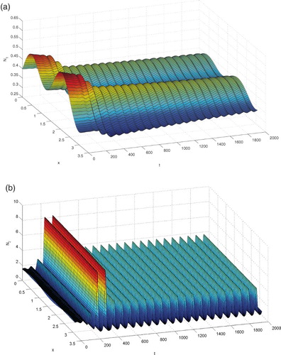Under the same initial values, now we choose $\tau =20>{\tau }_0^0$ and plot the graphs of $N_1(t,x)$ and $N_2(t,x)$ in Figure 2. From Figure 2, we see that there exists a family temporal periodic solutions, which implies that Hopf bifurcation occurs for system (38(38) $\begin{array}{rl}\frac{\mathrm{\partial }{N}_1(t,x)}{\mathrm{\partial }t}& =0.001N_1(t,x)+\frac{0.001N_1(t,x)N_2(t,x)}{1+0.391625N_1(t,x)+0.391625N_2(t,x)}\\ & -0.001N_1(t,x)N_2(t,x)-0.001N_1^2(t,x),\\ \frac{\mathrm{\partial }{N}_2(t,x)}{\mathrm{\partial }t}& =2.735375\frac{{\mathrm{\partial }}^2{N}_2(t,x)}{\mathrm{\partial }{x}^2}+\frac{1.5635N_1(t-\tau ,x)N_2(t,x)}{1+0.391625N_1(t-\tau ,x)+0.391625N_2(t-\tau ,x)}\\ & -0.391625N_2(t,x),\\ N_1(t,x)& =0.427839\times (1+2\sin (3.732x)+0.13\sin (1.4142x-0.6\left)\right),\\ N_2(t,x)& =1.380211\times (1+2\sin (2.732x)+0.13\sin (0.74142x+0.5\left)\right),\\ \frac{\mathrm{\partial }{N}_1}{\mathrm{\partial }\nu }& =\frac{\mathrm{\partial }{N}_2}{\mathrm{\partial }\nu }=0,t\ge 0,x\in \mathrm{\partial \Omega }.\end{array}$(38) ) at ${\tau }_0^0.$

Figure 1. The positive equilibrium $E^{\ast }(0.427839,1.380211)$ is asymptotically stable when $\tau =10<{\tau }_0^0=12.518011$.

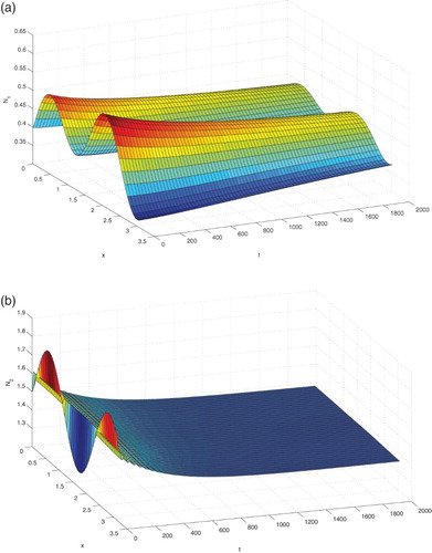
Figure 2. The temporal periodic solutions bifurcated from the equilibrium are stable, where $\tau =20>{\tau }_0^0=12.518011$.

5. Discussion

Various mathematical models have been proposed to study plant–pollinator population dynamics, see Soberon and Del Rio [24], Lundberg and Ingvarsson [19], Jang [14], Neuhauser and Fargione [20], Fishman and Hadany [8], Wang et al. [29], and Wang [26]. Most of these models are described by ordinary differential equations. Since pollinators travel between their nests and foraging patches, we believe that reaction–diffusion equations are more suitable to model the interactions between the plants and pollinators. We also assumed that there is a time delay in the process when the pollinators translate plant–pollinator interactions into the fitness and considered a plant–pollinator model with diffusion and time delay effects. As far as we know, there are no results for system (2(2) $\begin{array}{rl}\frac{\mathrm{\partial }{N}_1(t,x)}{\mathrm{\partial }t}& =N_1(t,x)\left[r_1+\frac{{\alpha }_{12}{N}_2(t,x)}{1+a{N}_1(t,x)+b{N}_2(t,x)}-{\beta }_1{N}_2(t,x)-d_1{N}_1(t,x)\right],\\ & x\in \mathrm{\Omega },t>0,\\ \frac{\mathrm{\partial }{N}_2(t,x)}{\mathrm{\partial }t}& =D_2\mathrm{\Delta }{N}_2(t,x)+N_2(t,x)\left[\frac{{\alpha }_{21}{N}_1(t-\tau ,x)}{1+a{N}_1(t-\tau ,x)+b{N}_2(t-\tau ,x)}-d_2\right],\\ & x\in \mathrm{\Omega },t>0,\\ N_1(t,x)& =\phi (t,x)\ge 0,N_2(t,x)=\psi (t,x)\ge 0,(t,x)\in [-\tau ,0]\times \overline{\mathrm{\Omega }},\\ \frac{\mathrm{\partial }{N}_1}{\mathrm{\partial }\nu }& =\frac{\mathrm{\partial }{N}_2}{\mathrm{\partial }\nu }=0,t\ge 0,x\in \mathrm{\partial \Omega },\end{array}$(2) ) with diffusion and time delay.

Firstly, by considering the distribution of eigenvalues of the corresponding linearized equation, stability of the positive constant steady-state and existence of spatially homogeneous and spatially inhomogeneous periodic solutions were studied. Secondly, by applying the normal form theory and the centre manifold reduction for partial functional differential equations, an explicit formula for determining the direction and stability of the Hopf bifurcation was given. Finally, to explain the obtained results, numerical simulations were presented.

Our results showed that if ${\alpha }_{21}>a{d}_2$ and either $\left(A1\right)$ $a_1<0,a_1^2-4a_0{a}_2=0$ or $\left(A2\right)$ $4a_0{a}_2<0$ holds, where $\begin{array}{rl}{a}_0& =\frac{b{\beta }_1}{{\alpha }_{21}-a{d}_2}+\frac{{\mathrm{d}}_1{d}_2{b}^2}{({\alpha }_{21}-a{d}_2{)}^2},a_1=\frac{{\beta }_1-b{r}_1}{{\alpha }_{21}-a{d}_2}+\frac{2d_1{d}_{2}b}{({\alpha }_{21}-a{d}_2{)}^2}-\frac{{\alpha }_{12}}{{\alpha }_{21}},\\ a_2& =-\frac{r_1}{{\alpha }_{21}-a{d}_2}+\frac{{\mathrm{d}}_1{d}_2}{({\alpha }_{21}-a{d}_2{)}^2},\end{array}$ then system (2(2) $\begin{array}{rl}\frac{\mathrm{\partial }{N}_1(t,x)}{\mathrm{\partial }t}& =N_1(t,x)\left[r_1+\frac{{\alpha }_{12}{N}_2(t,x)}{1+a{N}_1(t,x)+b{N}_2(t,x)}-{\beta }_1{N}_2(t,x)-d_1{N}_1(t,x)\right],\\ & x\in \mathrm{\Omega },t>0,\\ \frac{\mathrm{\partial }{N}_2(t,x)}{\mathrm{\partial }t}& =D_2\mathrm{\Delta }{N}_2(t,x)+N_2(t,x)\left[\frac{{\alpha }_{21}{N}_1(t-\tau ,x)}{1+a{N}_1(t-\tau ,x)+b{N}_2(t-\tau ,x)}-d_2\right],\\ & x\in \mathrm{\Omega },t>0,\\ N_1(t,x)& =\phi (t,x)\ge 0,N_2(t,x)=\psi (t,x)\ge 0,(t,x)\in [-\tau ,0]\times \overline{\mathrm{\Omega }},\\ \frac{\mathrm{\partial }{N}_1}{\mathrm{\partial }\nu }& =\frac{\mathrm{\partial }{N}_2}{\mathrm{\partial }\nu }=0,t\ge 0,x\in \mathrm{\partial \Omega },\end{array}$(2) ) has a unique positive constant steady-state $E^{\ast }(N_1^{\ast },N_2^{\ast }),$ in which $N_1^{\ast }=\frac{2a_0{d}_2-a_{1}b{d}_2+b{d}_2\sqrt{a_1^2-4a_0{a}_2}}{2a_0({\alpha }_{21}-a{d}_2)},N_2^{\ast }=\frac{-a_1+\sqrt{a_1^2-4a_0{a}_2}}{2a_0}.$ The first inequality ${\alpha }_{21}>a{d}_2$ ensures the existence of $a_0,a_1,a_2,$ and $N_1^{\ast }.$ Recall that ${\alpha }_{21}$ is regarded as the pollinators efficiency in translating plant–pollinator interactions into fitness, a is the effective constant for plant–pollinator interaction, and $d_2$ is the per-capita mortality rate of pollinators. This inequality means that the efficiency in translating plant–pollinator interactions into fitness of the pollinators must be greater than their mortality rate; otherwise the pollinators even cannot survive.

The inequality $a_1<0$ in (A1) is equivalent to $\frac{{\beta }_1-b{r}_1}{{\alpha }_{21}-a{d}_2}+\frac{2d_1{d}_{2}b}{({\alpha }_{21}-a{d}_2{)}^2}<\frac{{\alpha }_{12}}{{\alpha }_{21}},$ which indicates that the ratio of the efficiencies in translating plant–pollinator interactions into fitness of the plants and pollinators is greater than a certain value. In this case, an additional condition $a_1^2-4a_0{a}_2=0$ is needed to ensure the existence of $E^{\ast }(N_1^{\ast },N_2^{\ast }).$ Under the assumption (A2), it requires that $4a_0{a}_2<0.$ Note that now $a_0>0,$ so the condition is equivalent to $a_2<0,$ which, in turn, is equivalent to $r_1>\frac{{\mathrm{d}}_1{d}_2}{{\alpha }_{21}-a{d}_2}.$ The last inequality means that the intrinsic growth rate $r_1$ of the plants must be large enough compared to the death rates of the plants and pollinators.

We were interested in not only the effect of diffusion but also the effect of delay [4,12,31]. We found that system (2(2) $\begin{array}{rl}\frac{\mathrm{\partial }{N}_1(t,x)}{\mathrm{\partial }t}& =N_1(t,x)\left[r_1+\frac{{\alpha }_{12}{N}_2(t,x)}{1+a{N}_1(t,x)+b{N}_2(t,x)}-{\beta }_1{N}_2(t,x)-d_1{N}_1(t,x)\right],\\ & x\in \mathrm{\Omega },t>0,\\ \frac{\mathrm{\partial }{N}_2(t,x)}{\mathrm{\partial }t}& =D_2\mathrm{\Delta }{N}_2(t,x)+N_2(t,x)\left[\frac{{\alpha }_{21}{N}_1(t-\tau ,x)}{1+a{N}_1(t-\tau ,x)+b{N}_2(t-\tau ,x)}-d_2\right],\\ & x\in \mathrm{\Omega },t>0,\\ N_1(t,x)& =\phi (t,x)\ge 0,N_2(t,x)=\psi (t,x)\ge 0,(t,x)\in [-\tau ,0]\times \overline{\mathrm{\Omega }},\\ \frac{\mathrm{\partial }{N}_1}{\mathrm{\partial }\nu }& =\frac{\mathrm{\partial }{N}_2}{\mathrm{\partial }\nu }=0,t\ge 0,x\in \mathrm{\partial \Omega },\end{array}$(2) ) without delay cannot undergo Hopf bifurcations at the positive constant steady-state. But, under certain conditions, system (2(2) $\begin{array}{rl}\frac{\mathrm{\partial }{N}_1(t,x)}{\mathrm{\partial }t}& =N_1(t,x)\left[r_1+\frac{{\alpha }_{12}{N}_2(t,x)}{1+a{N}_1(t,x)+b{N}_2(t,x)}-{\beta }_1{N}_2(t,x)-d_1{N}_1(t,x)\right],\\ & x\in \mathrm{\Omega },t>0,\\ \frac{\mathrm{\partial }{N}_2(t,x)}{\mathrm{\partial }t}& =D_2\mathrm{\Delta }{N}_2(t,x)+N_2(t,x)\left[\frac{{\alpha }_{21}{N}_1(t-\tau ,x)}{1+a{N}_1(t-\tau ,x)+b{N}_2(t-\tau ,x)}-d_2\right],\\ & x\in \mathrm{\Omega },t>0,\\ N_1(t,x)& =\phi (t,x)\ge 0,N_2(t,x)=\psi (t,x)\ge 0,(t,x)\in [-\tau ,0]\times \overline{\mathrm{\Omega }},\\ \frac{\mathrm{\partial }{N}_1}{\mathrm{\partial }\nu }& =\frac{\mathrm{\partial }{N}_2}{\mathrm{\partial }\nu }=0,t\ge 0,x\in \mathrm{\partial \Omega },\end{array}$(2) ) undergoes Hopf bifurcations at the positive constant steady-state under the effect of delay. Recall that $\begin{array}{rl}{\alpha }_1& =-d_1{N}_1^{\ast }-\frac{{\alpha }_{12}a{N}_1^{\ast }{N}_2^{\ast }}{(1+a{N}_1^{\ast }+b{N}_2^{\ast }{)}^2}<0,{\alpha }_2=\frac{{\alpha }_{12}{N}_1^{\ast }(1+a{N}_1^{\ast })}{(1+a{N}_1^{\ast }+b{N}_2^{\ast }{)}^2}-{\beta }_1{N}_1^{\ast },\\ {\gamma }_1& =\frac{{\alpha }_{21}{N}_2^{\ast }(1+b{N}_2^{\ast })}{(1+a{N}_1^{\ast }+b{N}_2^{\ast }{)}^2}>0,{\gamma }_2=-\frac{b{\alpha }_{21}{N}_1^{\ast }{N}_2^{\ast }}{(1+a{N}_1^{\ast }+b{N}_2^{\ast }{)}^2}<0.\end{array}$ Our results demonstrated that if ${\alpha }_1{\gamma }_2-{\alpha }_2{\gamma }_1>0,{\alpha }_1(D_2+{\gamma }_2)-{\alpha }_2{\gamma }_1<0,D_2^2+{\alpha }_1^2-{\gamma }_2^2>0$ then the positive equilibrium $E^{\ast }$ is locally asymptotically stable if the time delay is less than a critical value $\tau <{\tau }_0,$ unstable when $\tau >{\tau }_0,$ and a family of periodic solutions bifurcates from $E^{\ast }$ when τ passes through ${\tau }_0$ via Hopf bifurcation. Moreover, the direction, stability and period of the bifurcating periodic solutions can be determined analytically. Notice that Wang et al. [29] showed that the ODE model (2(2) $\begin{array}{rl}\frac{\mathrm{\partial }{N}_1(t,x)}{\mathrm{\partial }t}& =N_1(t,x)\left[r_1+\frac{{\alpha }_{12}{N}_2(t,x)}{1+a{N}_1(t,x)+b{N}_2(t,x)}-{\beta }_1{N}_2(t,x)-d_1{N}_1(t,x)\right],\\ & x\in \mathrm{\Omega },t>0,\\ \frac{\mathrm{\partial }{N}_2(t,x)}{\mathrm{\partial }t}& =D_2\mathrm{\Delta }{N}_2(t,x)+N_2(t,x)\left[\frac{{\alpha }_{21}{N}_1(t-\tau ,x)}{1+a{N}_1(t-\tau ,x)+b{N}_2(t-\tau ,x)}-d_2\right],\\ & x\in \mathrm{\Omega },t>0,\\ N_1(t,x)& =\phi (t,x)\ge 0,N_2(t,x)=\psi (t,x)\ge 0,(t,x)\in [-\tau ,0]\times \overline{\mathrm{\Omega }},\\ \frac{\mathrm{\partial }{N}_1}{\mathrm{\partial }\nu }& =\frac{\mathrm{\partial }{N}_2}{\mathrm{\partial }\nu }=0,t\ge 0,x\in \mathrm{\partial \Omega },\end{array}$(2) ) does not have periodic solutions and Wang et al. [25] proved that the unique positive steady-state solution of a reaction–diffusion plant–pollinator model is a global attractor. Our results thus indicate that the time delay causes bifurcations and induces temporal periodic patterns in the diffusive plant–pollinator model. Such properties have been observed in many delay differential equation models [5,16]. This is similar to the observation in our other work [18] that oscillations occur in age-structured resource–consumer (plant–pollinator) models.

Wang et al. [29] and Wang [26] indeed investigated three species plant–pollinator–robber models. Since the movement of the nectar robbers plays an important role in their invasibility and coexistence of all species, it will be very interesting to study the population dynamics of the three species diffusive plant–pollinator–robber models. We leave this for future consideration.

Disclosure statement

No potential conflict of interest was reported by the authors.

Additional information

Funding

This work was partially supported by NSFC (No. 11471044 and No. 11371058), the Fundamental Research Funds for the Central Universities, and NSF (DMS-1412454).

References

- V.D. Adams, D.L. DeAngelis, and R.A. Goldstein, Stability analysis of the time delay in a host-parasitoid model, J. Theor. Biol. 83 (1980), pp. 43–62. doi: 10.1016/0022-5193(80)90371-9
- J.R. Beddington, Mutual interference between parasites or predators and its effect on searching efficiency, J. Anim. Ecol. 44 (1975), pp. 331–340. doi: 10.2307/3866
- S.A. Chamberlain and J.N. Holland, Density-mediated, context-dependent consumer–resource interactions between ants and extrafloral nectar plants, Ecology 89 (2008), pp. 1364–1374. doi: 10.1890/07-1139.1
- S. Chen, J. Shi, and J. Wei, Global stability and Hopf bifurcation in a delayed diffusive Leslie–Gower predator–prey system, Inter. J. Bifur. Chaos 22 (2012), pp. 1250061-1-11.
- J.M. Cushing, Integrodifferential Equations and Delay Models in Population Dynamics, Lecture Notes in Biomathematics, Vol. 20, Springer-Verlag, Heidelberg, 1977.
- D.L. DeAngelis, R.A. Goldstein, and R.V. O'Neill, A model for trophic interaction, Ecology 56 (1975), pp. 881–892. doi: 10.2307/1936298
- T. Faria, Normal forms and Hopf bifurcation for partial differential equations with delays, Trans. Amer. Math. Soc. 352 (2000), pp. 2217–2238. doi: 10.1090/S0002-9947-00-02280-7
- M.A. Fishman and L. Hadany, Plant-pollinator population dynamics, Theor. Popul. Biol. 78 (2010), pp. 270–277. doi: 10.1016/j.tpb.2010.08.002
- J.K. Hale, Theory of Functional Differential Equations, Springer-Verlag, Berlin, 1977.
- B.D. Hassard, N.D. Kazarinoff, and Y.-H. Wan, Theory and Application of Hopf Bifurcation, Cambridge University Press, Cambridge, 1981.
- J.N. Holland and D.L. DeAngelis, Consumer–resource theory predicts dynamic transitions between outcomes of interspecific interactions, Ecol. Lett. 12 (2009), pp. 1357–1366. doi: 10.1111/j.1461-0248.2009.01390.x
- G. Hu and W.-T. Li, Hopf bifurcation analysis for a delayed predator–prey system with diffusion effects, Nonlinear Anal. Real World Appl. 11 (2010), pp. 819–826. doi: 10.1016/j.nonrwa.2009.01.027
- S.S. Hu, D.L. Dilcher, D.M. Jarzen, and D.W. Taylor, Early steps of angiosperm pollinator coevolution, Proc. Natl. Acad. Sci. USA 105 (2008), pp. 240–245. doi: 10.1073/pnas.0707989105
- S.R.-J. Jang, Dynamics of herbivore–plant–pollinator models, J. Math. Biol. 44 (2002), pp. 129–149. doi: 10.1007/s002850100117
- C.A. Kearns, D.W. Inouye, and N.M. Waser, Endangered mutualisms: The conservation of plant–pollinator interactions, Annu. Rev. Ecol. Syst. 29 (1998), pp. 83–112. doi: 10.1146/annurev.ecolsys.29.1.83
- Y. Kuang, Delay Differential Equations with Applications in Population Dynamics, Academic Press, New York, 1993.
- X. Li, H. Wang, and Y. Kuang, Global analysis of a stoichiometric producer–grazer model with Holling type functional responses, J. Math. Biol. 63 (2011), pp. 901–932. doi: 10.1007/s00285-010-0392-2
- Z. Liu, P. Magal, and S. Ruan, Oscillations in age-structured models of consumer–resource mutualisms, Discret Contin. Dyn. Syst. B 21 (2016), pp. 537–555. doi: 10.3934/dcdsb.2016.21.537
- S. Lundberg and P. Ingvarsson, Population dynamics of resource limited plants and their pollinators, Theor. Popul. Biol. 54 (1998), pp. 44–49. doi: 10.1006/tpbi.1997.1349
- C. Neuhauser and J.E. Fargione, A mutualism–parasitism continuum model and its application to plant–mycorrhizae interactions, Ecol. Model. 177 (2004), pp. 337–352. doi: 10.1016/j.ecolmodel.2004.02.010
- E.R. Pianka, Evolutionary Ecology, Harper and Row, New York, 1974.
- S. Ruan, Absolute stability, conditional stability and bifurcation in Kolmogorov-type predator–prey systems with discrete delays, Quart. Appl. Math. 59 (2001), pp. 159–173.
- S. Ruan and J. Wei, On the zeros of a third degree exponential polynomial with applications to a delayed model for the control of testosterone secretion, IMA J. Math. Appl. Med. Biol. 18 (2001), pp. 41–52. doi: 10.1093/imammb/18.1.41
- J .M. Soberon and C.M. Del Rio, The dynamics of a plant-pollinator interaction, J. Theor. Biol. 91 (1981), pp. 363–378. doi: 10.1016/0022-5193(81)90238-1
- L. Wang, H. Jiang and Y. Li, Positive steady state solutions of a plant-pollinator model with diffusion, Discret. Contin. Dyn. Syst. B 20 (2015), pp. 1805–1819. doi: 10.3934/dcdsb.2015.20.1805
- Y. Wang, Dynamics of plant-pollinator-robber systems, J. Math. Biol. 66 (2013), pp. 1155–1177. doi: 10.1007/s00285-012-0527-8
- Y. Wang and D.L. DeAngelis, Transitions of interaction outcomes in a uni-directional consumer–resource system, J. Theor. Biol. 208 (2011), pp. 43–49. doi: 10.1016/j.jtbi.2011.03.038
- Y. Wang, D.L. DeAngelis, and J.N. Holland, Uni-directional consumer–resource theory characterizing transitions of interaction outcomes, Ecol. Complex. 8 (2011), pp. 249–257. doi: 10.1016/j.ecocom.2011.04.002
- Y. Wang, D.L. DeAngelis, and J.N. Holland, Uni-direction interation and plant-pollinator-robber coexistence, Bull. Math. Biol. 74 (2012), pp. 2142–2164. doi: 10.1007/s11538-012-9750-0
- J. Wu, Theory and Applications of Partial Functional Differential Equations, Springer-Verlag, New York, 1996.
- W. Zuo and J. Wei, Stability and Hopf bifurcation in a diffusive predator–prey system with delay effect, Nonlinear Anal. Real World Appl. 12 (2011), pp. 1998–2011. doi: 10.1016/j.nonrwa.2010.12.016