Analysis of a model of gambiense sleeping sickness in humans and cattle

ABSTRACT

Human African Trypanosomiasis (HAT) and Nagana in cattle, commonly called sleeping sickness, is caused by trypanosome protozoa transmitted by bites of infected tsetse flies. We present a deterministic model for the transmission of HAT caused by Trypanosoma brucei gambiense between human hosts, cattle hosts and tsetse flies. The model takes into account the growth of the tsetse fly, from its larval stage to the adult stage. Disease in the tsetse fly population is modeled by three compartments, and both the human and cattle populations are modeled by four compartments incorporating the two stages of HAT. We provide a rigorous derivation of the basic reproduction number ${\mathcal{R}}_0$. For ${\mathcal{R}}_0<1$, the disease free equilibrium is globally asymptotically stable, thus HAT dies out; whereas (assuming no return to susceptibility) for ${\mathcal{R}}_0>1$, HAT persists. Elasticity indices for ${\mathcal{R}}_0$ with respect to different parameters are calculated with baseline parameter values appropriate for HAT in West Africa; indicating parameters that are important for control strategies to bring ${\mathcal{R}}_0$ below 1. Numerical simulations with ${\mathcal{R}}_0>1$ show values for the infected populations at the endemic equilibrium, and indicate that with certain parameter values, HAT could not persist in the human population in the absence of cattle.

KEYWORDS:

• Trypanosoma brucei gambiense
• sleeping sickness
• vector-borne disease
• global stability
• elasticity

2010 MATHEMATICS SUBJECT CLASSIFICATION:

• 92D30
• 34D23

1. Introduction

Human African trypanosomiasis (HAT) and Nagana in cattle is generally known as sleeping sickness. It is a serious parasitic disease that affects 36 sub-Saharan Africa countries, threatening the life of millions of people in rural settlements. Sleeping disorders, the origin of its name, are a key feature of the advanced stage of the disease when the central nervous system is affected. In the absence of treatment, the outcome is usually fatal; see, for example, Rock et al. [20]. The trypanosome protozoa causing the disease are transmitted to humans or cattle by the bite of an infected tsetse fly. There are two different types of human sleeping sickness that are caused by two different subspecies of trypanosomes: gambiense sleeping sickness, caused by Trypanosoma brucei gambiense (T. b. gambiense) transmitted by flies of the Glossina palpalis group, is generally considered to be a chronic disease and is found mostly in West and Central Africa; and rhodesiense sleeping sickness, caused by Trypanosoma brucei rhodesiense, transmitted by flies of the Glossina morsitans group, is an acute disease that occurs mainly in East Africa [20]. Gambiense sleeping sickness constitutes 98% of all the cases declared, and the most affected country is the Democratic Republic of the Congo, with more than 75% of the recorded gambiense cases [10].

The first descriptions of sleeping sickness are from what is known now as Mali. Travelers recognized the symptoms but were unaware of the relationship with the tsetse fly. We are indebted to Aldo Castellani, for his renowned work on identification of the trypanosoma as the causal agent of sleeping sickness [6]. For a long time, African farmers knew from experience that there was a link between biting flies and outbreaks of trypanosomiasis or Nagana in their livestock. But this link was formally established for the first time by David Bruce [4], who worked in what is now Kwazulu Natal, South Africa. He observed that cattle and healthy dogs sent into tsetse fly infested areas caught the same parasite in the blood and got sick, suggesting that Nagana was the same as the ‘tsetse disease’. A review of wildlife infested tsetse fly regions showed that trypanosomes were also in their blood, leading Bruce to suggest that this disease could be eradicated by destroying wildlife. The existence of the life cycle of the parasite in the insect was found after 16 years of research [5].

Tsetse flies, which are the vectors of HAT and Nagana, are large and robust biting flies that are common in sub-Saharan African between the Sahara and the Kalahari Deserts. The life cycle of the tsetse fly is very unusual because it does undergo a total metamorphosis (i.e. eggs, larvae, pupae and adults), but only a single larva develops in the uterus of the female fly at any given time [10]. Tsetse flies are obligate hematophagous insects, meaning both male and female flies survive purely on a diet of blood. Female tsetse flies mate just once, almost immediately after emergence from their puparium. In the wild, mating probably occurs close to, or even on, the host animal around the time of the female's first blood meal. She produces a single egg at a time, which develops within her uterus into a fully developed larva that she places on the ground nine days later [20, 23]. Once laid, the larval stage is only of very short duration (a few minutes), just the time it takes for the larva to burrow itself into the ground where it immediately becomes a pupa. The fly emerges 22–60 days later, depending on the temperature. Once the female fly has fed and mated, the whole cycle begins again. The mother tsetse fly will continue to produce a single larva at roughly 10- to 12-day intervals for her entire life [23]. During her life-span a female can theoretically give birth to only a maximum of 8–10 offspring (in reality much lower). Wild male tsetse can achieve a life-span of almost 5 months (but in reality, very rarely that long). When a tsetse fly bites humans or cattle, trypanosomiasis can be transmitted to humans or to cattle by an infectious fly. Trypanosomiasis in humans and cattle progresses from haemolymphatic (stage I) to meningoencephalitic (stage II), over a period of a few months to several years [16, 20]. The first stage of sleeping sickness in humans presents with non-specific symptoms, such as fever, headache and joint pain. Often first stage infected humans are unaware that they are infected and they continue to do their daily activities where they can be bitten by tsetse flies; whereas in the second stage infected humans are usually very sick with neurological symptoms and are bed bound. In infected areas, screening campaigns to detect patients in the first stage of HAT are often conducted, and once humans become symptomatic (stage II) they are offered treatment by drugs [20]. There have been reports of vertical transmission from infectious human mothers to their babies, however the risk is unknown and under reported [16]. Trypanosomiasis can be transmitted to a biting fly from an infectious host in the first or second stage of the disease.

Compartmental modelling of vector-borne diseases began with the Ross–Macdonald model [17, 22]; see, for example, Anderson and May [1, Section 14.3], which is a two-dimensional model for malaria. In 1988, Rogers [21] extended this model to make it more relevant for West African trypanosomiases transmitted by T. b. gambiense by including more than one host species (e.g. domestic animals and humans), an incubation period and a period of temporary immunity for the human host, a probability of disease transmission from a bite by a susceptible fly on an infectious host, and survival of a vector between being infected and transmitting infection. Analysis of the resulting three-dimensional model included determining a disease threshold, the equilibrium disease prevalence, and evaluating these for data appropriate for a West African village. A five variable compartmental model for the dynamics of HAT including tsetse flies and humans was formulated by Artzrouni and Gouteux [3]. They included susceptible, incubating, asymptomatic and removed humans, and compared their model results with data from the Democratic Republic of Congo. In a subsequent paper, these authors [2] used their model to compare control strategies. Chalvet-Monfray et al. [7] then extended this to two patches, to model a village and plantations. More recently Hargrove et al. [13] modelled the control of trypanosomiasis caused by T. b. rhodiense in multiple hosts. Their model predicted that treating cattle with insecticide is generally more effective than treating cattle with drugs. Kajunguri et al. [14] also formulated a multi-host model for HAT caused by T. b. rhodiense, and in particular found that restricted application of insecticide to cattle on only their legs and belly (favoured tsetse feeding sites) provides a cost-effective method of control. Funk et al. [12] developed a multiple host model for gambiense HAT and provided field data estimates of the basic reproduction number in Bipindi, Cameroon. A very recent comprehensive survey and reference list on mathematical models of HAT epidemiology is provided by Rock et al. [20], where they also stress the need for further model development to understand HAT transmission and to suggest control strategies. In fact, in 2012, the World Health Organization set a target date of 2020 for HAT elimination [25]. Current strategies for controlling and eliminating gambiense HAT are reviewed by Steinmann et al. [28].

Our model of gambiense HAT includes the life cycle of tsetse flies, incubation periods for both flies, humans and cattle (which may include domestic livestock and wild animals) and cross transmission between vector and hosts. As in Funk et al. [12], we assume that both humans and cattle are hosts for T. b. gambiense. We give a mathematical analysis of our model, presenting a rigorous derivation of the basic reproduction number and some new global stability results. By proposing a general model that can be adapted to suit different settings and scenarios, our objective is to contribute to the understanding of the transmission dynamics of HAT and provide tools to suggest strategies for control. This paper is structured as follows. We introduce the model in Section 2 by considering the growth dynamics of the tsetse fly, the transmission dynamics of the tsetse fly and the human and cattle host populations. In Section 3, we calculate the basic reproduction number, and study the stability of the disease free equilibrium (DFE). We also prove in Section 3 that there exists a globally asymptotically stable endemic equilibrium in the case in which return to susceptibility is ignored. In Section 4, parameter values collected from the literature on HAT are used to calculate elasticity indices and to compute numerical solutions of our model. We draw our conclusions in Section 5.

2. Model formulation

2.1. Modelling the dynamics of growth of the tsetse fly

We first model the growth dynamics of the tsetse fly. From the life cycle described in Section 1, it is sufficient to consider two life stages, namely pupal and adult flies. A similar approach is given in [19] in which three life stages of mosquitoes are taken in a model for chikungunya.

Let $L\left(t\right)$ be the number of pupae at time t and $A\left(t\right)$ be the number of (male and female) adult flies at time t. The dynamics of L and A are modelled by the following system: (1) $\begin{array}{rl}\frac{\mathrm{d}L}{\mathrm{d}t}& =b_{L}WA\left(1-\frac{L}{K_L}\right)-({\sigma }_L+d_L)L,\end{array}$(1) (2) $\begin{array}{rl}\frac{\mathrm{d}A}{\mathrm{d}t}& ={\sigma }_{L}L-d_{F}A.\end{array}$(2) Here, $b_L$ is the rate at which female flies give birth to larvae; W is the proportion of female flies in the population of adult flies; $K_L$ is the pupal carrying capacity of the nesting site; ${\sigma }_L$ is the transfer rate of pupae into adult tsetse flies, so $1/{\sigma }_L$ is the average time as a pupa; $d_L$ and $d_F$ are the mortality rate of pupae and adult flies, respectively; with all parameters assumed positive.

2.1.1. Equilibrium points.

The threshold defined by (3) $r=\frac{{\sigma }_L}{{\sigma }_L+d_L}\frac{b_{L}W}{d_F},$(3) is important when calculating equilibrium points of system (1(1) $\begin{array}{rl}\frac{\mathrm{d}L}{\mathrm{d}t}& =b_{L}WA\left(1-\frac{L}{K_L}\right)-({\sigma }_L+d_L)L,\end{array}$(1) )–(2(2) $\begin{array}{rl}\frac{\mathrm{d}A}{\mathrm{d}t}& ={\sigma }_{L}L-d_{F}A.\end{array}$(2) ), as shown in the following result. The parameter r can be interpreted as the probability of surviving the pupal stage multiplied by the birth rate divided by the death rate.

Proposition 1

Let $D=\left\{(L,A)\in {\mathbb{R}}_{+}^2|0\le L\le K_L,0\le A\le \frac{{\sigma }_L}{d_F}{K}_L\right\}.$

1. The set D is positively invariant with respect to the system (1(1) $\begin{array}{rl}\frac{\mathrm{d}L}{\mathrm{d}t}& =b_{L}WA\left(1-\frac{L}{K_L}\right)-({\sigma }_L+d_L)L,\end{array}$(1) )–(2(2) $\begin{array}{rl}\frac{\mathrm{d}A}{\mathrm{d}t}& ={\sigma }_{L}L-d_{F}A.\end{array}$(2) ), whenever the initial conditions lie in $\mathrm{int}\left(D\right)$.

2. The system (1(1) $\begin{array}{rl}\frac{\mathrm{d}L}{\mathrm{d}t}& =b_{L}WA\left(1-\frac{L}{K_L}\right)-({\sigma }_L+d_L)L,\end{array}$(1) )–(2(2) $\begin{array}{rl}\frac{\mathrm{d}A}{\mathrm{d}t}& ={\sigma }_{L}L-d_{F}A.\end{array}$(2) ) always has a trivial fly-free equilibrium $(L,A)=(0,0)$. If $r\le 1,$ this is the only equilibrium. If $r>1,$ then there is a unique positive equilibrium with larvae and adults present given by (4) $(L^{\ast },A^{\ast })=\left(1-\frac{1}{r}\right)K_L\left(1,\frac{{\sigma }_L}{d_F}\right).$(4)

3. If $r<1,$ then the equilibrium point $(0,0)$ is globally asymptotically stable in D.

4. If $r>1,$ then the equilibrium $(L^{\ast },A^{\ast })$ defined by (4(4) $(L^{\ast },A^{\ast })=\left(1-\frac{1}{r}\right)K_L\left(1,\frac{{\sigma }_L}{d_F}\right).$(4) ) is globally asymptotically stable in $\mathrm{int}\left(D\right)$.

Proof.

Parts (i) and (ii) follow easily from the system (1(1) $\begin{array}{rl}\frac{\mathrm{d}L}{\mathrm{d}t}& =b_{L}WA\left(1-\frac{L}{K_L}\right)-({\sigma }_L+d_L)L,\end{array}$(1) )–(2(2) $\begin{array}{rl}\frac{\mathrm{d}A}{\mathrm{d}t}& ={\sigma }_{L}L-d_{F}A.\end{array}$(2) ).

Linearizing the system (1(1) $\begin{array}{rl}\frac{\mathrm{d}L}{\mathrm{d}t}& =b_{L}WA\left(1-\frac{L}{K_L}\right)-({\sigma }_L+d_L)L,\end{array}$(1) )–(2(2) $\begin{array}{rl}\frac{\mathrm{d}A}{\mathrm{d}t}& ={\sigma }_{L}L-d_{F}A.\end{array}$(2) ) about an equilibrium, gives the Jacobian matrix (5) $J=\left(\begin{array}{cc}-\frac{b_{L}WA}{K_L}-({\sigma }_L+d_L)& b_{L}W\left(1-\frac{L}{K_L}\right)\\ {\sigma }_L& -d_F\end{array}\right),$(5) where $(L,A)=(0,0)$ or $(L^{\ast },A^{\ast })$.

For part (iii), when $(L,A)=(0,0)$, the characteristic equation of J is ${\lambda }^2+({\sigma }_L+d_L+d_F)\lambda +({\sigma }_L+d_L)d_F(1-r)=0,$ which implies that $(0,0)$ is locally asymptotically stable if $r<1.$ Global asymptotic stability for r<1 is proved using the Lyapunov function $V=\left(d_F/b_{L}W\right)L+A$, giving $\dot{V}=-d_F\left(AL/K_L\right)-{\sigma }_L(1/r-1)L\le 0$, and using LaSalle's invariance principle.

For part (iv), if r>1 then (5(5) $J=\left(\begin{array}{cc}-\frac{b_{L}WA}{K_L}-({\sigma }_L+d_L)& b_{L}W\left(1-\frac{L}{K_L}\right)\\ {\sigma }_L& -d_F\end{array}\right),$(5) ) at $(L^{\ast },A^{\ast })$ has the characteristic equation ${\lambda }^2+\left(b_{L}W\left(1-\frac{1}{r}\right)\frac{{\sigma }_L}{d_F}+({\sigma }_L+d_L)+d_F\right)\lambda +b_{L}W{\sigma }_L+({\sigma }_L+d_L)d_F=0,$ which implies that $(L^{\ast },A^{\ast })$ is locally asymptotically stable. The Bendixson–Dulac criterion on the system (1(1) $\begin{array}{rl}\frac{\mathrm{d}L}{\mathrm{d}t}& =b_{L}WA\left(1-\frac{L}{K_L}\right)-({\sigma }_L+d_L)L,\end{array}$(1) )–(2(2) $\begin{array}{rl}\frac{\mathrm{d}A}{\mathrm{d}t}& ={\sigma }_{L}L-d_{F}A.\end{array}$(2) ) shows that there can be no periodic solution in D. Thus the Poincaré–Bendixson theorem; see, for example [[26, p. 9], [9, Theorem 1, p. 327, 329]], shows that the unique positive equilibrium $(L^{\ast },A^{\ast })$ is globally asymptotically stable in $\mathrm{int}\left(D\right)$.

2.2. Formulation of the full model

2.2.1. Modelling transmission dynamics of the tsetse fly and the host populations

Tsetse flies become infected by biting infectious vertebrate hosts. Then infectious tsetse flies infect susceptible hosts when they take future blood meals. We model the dynamics of the population of vectors as described by the system (1(1) $\begin{array}{rl}\frac{\mathrm{d}L}{\mathrm{d}t}& =b_{L}WA\left(1-\frac{L}{K_L}\right)-({\sigma }_L+d_L)L,\end{array}$(1) )–(2(2) $\begin{array}{rl}\frac{\mathrm{d}A}{\mathrm{d}t}& ={\sigma }_{L}L-d_{F}A.\end{array}$(2) ), with the evolution of this system governed by the threshold r defined in (3(3) $r=\frac{{\sigma }_L}{{\sigma }_L+d_L}\frac{b_{L}W}{d_F},$(3) ). If r<1, the population of tsetse flies will be extinguished, otherwise they evolve toward an equilibrium given by (4(4) $(L^{\ast },A^{\ast })=\left(1-\frac{1}{r}\right)K_L\left(1,\frac{{\sigma }_L}{d_F}\right).$(4) ). For our full model, we assume that r>1 and that the flies are at the equilibrium $(L^{\ast },A^{\ast })$. Trypanosomiasis in the fly population is modelled by an SEI compartmental model. It is assumed that a fly once infected will never recover or be removed. So we subdivide the adult fly population into three compartments, $S_F$ susceptible tsetse flies, $E_F$ exposed tsetse flies infected but not yet infectious and $I_F$ infectious tsetse flies that are able to transmit the disease once they bite a susceptible host. Thus the total adult fly population is (6) $A^{\ast }=S_F+E_F+I_F.$(6)

The human and cattle host populations are described by a Malthus model. We denote by $N_H$ and $N_C$ the total size of the human and cattle host populations, respectively, at time t and $b_H,b_C,d_H,d_C$ are the rates of birth and mortality of the human and cattle host populations, respectively. The dynamics of $N_H$ and $N_C$ are governed by (7) $\begin{array}{rl}\frac{\mathrm{d}{N}_H}{\mathrm{d}t}& =(b_H-d_H)N_H={\alpha }_H{N}_H,\end{array}$(7) (8) $\begin{array}{rl}\frac{\mathrm{d}{N}_C}{\mathrm{d}t}& =(b_C-d_C)N_C={\alpha }_C{N}_C,\end{array}$(8) where ${\alpha }_H=b_H-d_H$ and ${\alpha }_C=b_C-d_C$ are the growth rates of the human and cattle population respectively. If ${\alpha }_H<0({\alpha }_C<0)$, the human (cattle) population will be extinguished, it will remain constant if ${\alpha }_H=0({\alpha }_C=0)$, and will grow exponentially if ${\alpha }_H>0({\alpha }_C>0)$. We assume that ${\alpha }_H=0({\alpha }_C=0)$, i.e. $b_H=d_H$$(b_C=d_C)$, so that the human (cattle) population is constant over the period of the study and there is no human and cattle death due to HAT.

Trypanosomiasis in the human and cattle host populations is modelled with four compartments in each population:

• susceptible hosts $S_H\left(S_C\right)$, humans (cattle) who are at risk and free of the disease;

• exposed hosts $E_H\left(E_C\right)$, humans (cattle) who are in the latent stage of the disease, they are infected but unable to transmit the disease;

• infectious hosts $I_H\left(I_C\right)$, humans (cattle) who are able to transmit the disease to tsetse flies if they are bitten [12]. These compartments contain hosts in the first stage of the disease unaware they are infected or with only minor symptoms; and

• removed hosts $R_H\left(R_C\right)$, consisting of humans (cattle) in the second stage of the disease who are very sick and not exposed to flies, so that they do not pass on infection, as well as humans (cattle) who are undergoing treatment and are also not exposed to flies. We assume that treatment commences at the beginning of stage II, as this is usually when hosts become symptomatic. These compartments also contain removed humans (cattle) that have developed temporary immunity after recovery from stage II or treatment and they can neither transmit nor acquire HAT, but they will become susceptible again after the period of temporary immunity has lapsed.

The constant total human and cattle populations are defined by (9) $\begin{array}{rl}{N}_H& =S_H+E_H+I_H+R_H,\end{array}$(9) (10) $\begin{array}{rl}{N}_C& =S_C+E_C+I_C+R_C.\end{array}$(10)

The dynamics of T. b. gambiense in the tsetse fly population, assuming that transmission to flies occurs from humans and cattle in only the first stage of HAT, is given by the system (11) $\begin{array}{rl}\frac{\mathrm{d}{S}_F}{\mathrm{d}t}& ={\sigma }_L{L}^{\ast }-d_F{S}_F-(1-p)ac\frac{I_H}{N_H}{S}_F-\mathit{\text{pav}}\frac{I_C}{N_C}{S}_F,\end{array}$(11) (12) $\begin{array}{rl}\frac{\mathrm{d}{E}_F}{\mathrm{d}t}& =(1-p)ac\frac{I_H}{N_H}{S}_F+\mathit{\text{pav}}\frac{I_C}{N_C}{S}_F-(q_F+d_F)E_F,\end{array}$(12) (13) $\begin{array}{rl}\frac{\mathrm{d}{I}_F}{\mathrm{d}t}& =q_F{E}_F-d_F{I}_F,\end{array}$(13) where $L^{\ast }$ is the number of pupae at equilibrium given by (4(4) $(L^{\ast },A^{\ast })=\left(1-\frac{1}{r}\right)K_L\left(1,\frac{{\sigma }_L}{d_F}\right).$(4) ), a is the vector blood feeding rate, c is the probability that a fly becomes infected after biting an infectious human, v is the probability that a fly becomes infected after biting infectious cattle, $1/q_F$ is the incubation period in the fly, $d_F$ is the natural mortality rate of adult flies and p is the proportion of tsetse fly bites on cattle (thus $(1-p)$ is the proportion of bites on humans). This proportion is assumed to be constant as in Funk et al. [12]; for a discussion of this assumption see Rock et al. [20, Section 3.3].

The dynamics of T. b. gambiense in the human host population is governed by the system $\begin{array}{rl}\frac{\mathrm{d}{S}_H}{\mathrm{d}t}& =b_H{N}_H+{\kappa }_H{R}_H-(1-p)ab\frac{I_F}{N_H}{S}_H-b_H{S}_H,\\ \frac{\mathrm{d}{E}_H}{\mathrm{d}t}& =(1-p)ab\frac{I_F}{N_H}{S}_H-(q_H+b_H)E_{H,}\\ \frac{\mathrm{d}{I}_H}{\mathrm{d}t}& =q_H{E}_H-({\gamma }_H+b_H)I_H,\\ \frac{\mathrm{d}{R}_H}{\mathrm{d}t}& ={\gamma }_H{I}_H-(b_H+{\kappa }_H)R_H,\end{array}$ where b is the probability that an infectious fly infects a human host, $b_H$ is the birth rate of the human population, $d_H=b_H$ is the human mortality rate, $1/q_H$ is the average incubation period for a human host, $1/{\gamma }_H$ is the average length of stage I for humans corresponding to the infectious period. For untreated humans, $1/{\kappa }_H$ is the sum of the average length of stage II and the average temporary immunity period. For treated humans, $1/{\kappa }_H$ is the sum of the average length of treatment and the average temporary immunity period. Note that we assume that the average length of treatment is equal to the average length of stage II. Similarly, the dynamics of T. b. gambiense in the cattle host population is governed by the system $\begin{array}{rl}\frac{\mathrm{d}{S}_C}{\mathrm{d}t}& =b_C{N}_C+{\kappa }_C{R}_C-\mathit{\text{pau}}\frac{I_F}{N_C}{S}_C-b_C{S}_C,\\ \frac{\mathrm{d}{E}_C}{\mathrm{d}t}& =\mathit{\text{pau}}\frac{I_F}{N_C}{S}_C-(q_C+b_C)E_C,\\ \frac{\mathrm{d}{I}_C}{\mathrm{d}t}& =q_C{E}_C-({\gamma }_C+b_C)I_C,\\ \frac{\mathrm{d}{R}_C}{\mathrm{d}t}& ={\gamma }_C{I}_C-(b_C+{\kappa }_C)R_C.\end{array}$ where u is the probability that an infectious fly infects a cattle host, $b_C$ is the birth rate of the cattle population, $d_C=b_C$ is the cattle mortality rate $1/q_C$ is the average incubation period for cattle, $1/{\gamma }_C$ is the average length of stage I for cattle corresponding to the infectious period. For untreated cattle, $1/{\kappa }_C$ is the sum of the average length of stage II and the average temporary immunity period. For treated cattle, $1/{\kappa }_C$ is the sum of the average length of treatment and the average temporary immunity period. As in humans, we assume that the average length of treatment is equal to the average length of stage II for cattle.

Thus, the dynamics of the transmission of sleeping sickness are then described by the system of Equations (14(14) $\frac{\mathrm{d}{E}_F}{\mathrm{d}}t=(1-p)ac{\frac{I_H{N}_H}{S}}_F+pav{\frac{I_C{N}_C}{S}}_F-{\tilde{q}}_F{E}_F,$(14) )–(24(24) $\frac{\mathrm{d}{R}_C}{\mathrm{d}t}={\gamma }_C{I}_C-(b_C+{\kappa }_C)R_C,$(24) ), where we have assumed that there is no death due to the disease, no vertical transmission, and all parameters are positive, except that ${\kappa }_H$ and ${\kappa }_C$ are nonnegative. The equations are ordered with infected classes first. (14) $\frac{\mathrm{d}{E}_F}{\mathrm{d}}t=(1-p)ac{\frac{I_H{N}_H}{S}}_F+pav{\frac{I_C{N}_C}{S}}_F-{\tilde{q}}_F{E}_F,$(14) (15) $\frac{\mathrm{d}{I}_F}{\mathrm{d}}t=q_F{E}_F-d_F{I}_F,$(15) (16) $\frac{\mathrm{d}{E}_H}{\mathrm{d}}t=(1-p)ab{\frac{I_F{N}_H}{S}}_H-{\tilde{q}}_H{E}_H,$(16) (17) $\frac{\mathrm{d}{I}_H}{\mathrm{d}t}=q_H{E}_H-{\tilde{\gamma }}_H{I}_{H,}$(17) (18) $\frac{\mathrm{d}{E}_C}{\mathrm{d}t}=\mathit{\text{pau}}\frac{I_F}{N_C}{S}_C-{\tilde{q}}_C{E}_C,$(18) (19) $\frac{\mathrm{d}{I}_C}{\mathrm{d}t}=q_C{E}_C-{\tilde{\gamma }}_C{I}_C,$(19) (20) $\frac{\mathrm{d}{S}_F}{\mathrm{d}t}={\sigma }_L{L}^{\ast }-d_F{S}_F-(1-p)ac\frac{I_H}{N_H}{S}_F-\mathit{\text{pav}}\frac{I_C}{N_C}{S}_F,$(20) (21) $\frac{\mathrm{d}{S}_H}{\mathrm{d}t}=b_H{N}_H+{\kappa }_H{R}_H-(1-p)ab\frac{I_F}{N_H}{S}_H-b_H{S}_H,$(21) (22) $\frac{\mathrm{d}{S}_C}{\mathrm{d}t}=b_C{N}_C+{\kappa }_C{R}_C-\mathit{\text{pau}}\frac{I_F}{N_C}{S}_C-b_C{S}_C,$(22) (23) $\frac{\mathrm{d}{R}_H}{\mathrm{d}t}={\gamma }_H{I}_H-(b_H+{\kappa }_H)R_H,$(23) (24) $\frac{\mathrm{d}{R}_C}{\mathrm{d}t}={\gamma }_C{I}_C-(b_C+{\kappa }_C)R_C,$(24) where ${\tilde{\gamma }}_i={\gamma }_i+b_i,{\tilde{q}}_i=q_i+b_i$, for $i\in \{H,C\}$ and ${\tilde{q}}_F=q_F+d_F$.

Figure 1 shows a flow diagram for this system and Table 1 describes the model parameters. Note that all cross transmission terms are normalized with respect to the host population as is common in vector-borne disease models [1, Section 14.3]. Nonnegative initial conditions with $E_F\left(0\right)+I_F\left(0\right)+E_H\left(0\right)+I_H\left(0\right)+E_C\left(0\right)+I_C\left(0\right)$ positive and small, complete the formulation of our HAT model in the invariant region (25) $\mathrm{\Gamma }=\left\{(E_F,I_F,E_H,I_H,E_C,I_C,S_F,S_H,R_H,S_C,R_C)\in {\mathbb{R}}_{+}^{11}|\left\{\begin{array}{c}{E}_F+I_F+S_F=A^{\ast },\\ E_H+I_H+S_H+R_H=N_H\\ E_C+I_C+S_C+R_C=N_C\end{array}\right\}\right\}.$(25)

Figure 1. Flow diagram of HAT transmission dynamics.

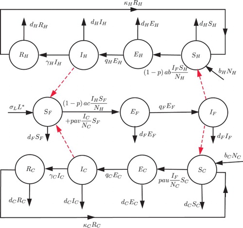
Figure 2. Numbers of humans, cattle and flies in each compartment with baseline parameter values as in Table 1 with $I_F=1$, $N_H=300$, $N_C=50$ and $L^{\ast }=4545$, giving approximate equilibrium values $S_C^{\ast }=5,E_C^{\ast }=5,I_C^{\ast }=10,R_C^{\ast }=30,S_H^{\ast }=165,E_H^{\ast }=12,I_H^{\ast }=31,R_H^{\ast }=92,S_F^{\ast }=4929,E_F^{\ast }=31,I_F^{\ast }=40$. For these parameter values, the reproduction numbers are ${\mathcal{R}}_0=3.0298,{\mathcal{R}}_{0H}=1.9051,{\mathcal{R}}_{0C}=4.2505$.

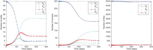
Table 1. Description of model parameters, indicating baselines, ranges and references. The first six parameters describing larval and adult fly populations are fixed at their baseline values.

Parameter	Description	Baseline value	Value range with time $\mathrm{unit}=1$ day
${\sigma }_L$	Rate of maturation from pupal to adult fly	$\frac{1}{30}$	$\frac{1}{60}$ to $\frac{1}{22}$ [18]
$d_F$	Fly death rate	$\frac{1}{33}$	$\frac{1}{30}$ to $\frac{1}{62}$ [3]
W	Proportion of female flies	$\frac{6}{10}$	Estimated guess, female flies are more abundant than males
$d_L$	Pupa death rate	$\frac{1}{100}$	Estimated guess, in natural conditions very few pupae die
$K_L$	Pupa carrying capacity	300,000	Estimated guess
$b_L$	Larva birth rate	$\frac{0.6}{9}$	An adult female is expected to produce one larva every 9 days. [18, 20]
$b_H$	Human population $\mathrm{birthrate}=\mathrm{deathrate}$	$\frac{1}{50\times 365}$	10 to 40 births per 1000 per year [14]
$b_C$	Cattle population $\mathrm{birthrate}=\mathrm{deathrate}$	$\frac{1}{15\times 365}$	Estimated guess
$q_F$	Incubation rate of the flies	$\frac{1}{25}$	$\frac{1}{25}$ to $\frac{1}{30}$ [[3], [21, Table 2]]
$q_H,q_C$	Incubation rate of humans, cattle	$\frac{1}{12}$	$\frac{1}{10}$ to $\frac{1}{14}$, incubation period is between 10 and 14 days [3]
a	Fly biting rate	$\frac{1}{4}$	$\frac{1}{10}$ to $\frac{1}{3}$, a fly is expected to have 1 bite every 3–10 days [21]
p	Proportion of tsetse fly bites on cattle	0.7	[21, Table 2]
b,u	Probability that an infectious fly infects a human, cattle	0.62	[21, Table 2]
c,v	Probability that a fly becomes infected after biting an infectious human, cattle	0.01	Estimated guess [21, Table 2]
${\gamma }_H,{\gamma }_C$	Human, cattle rate of progression from stage I to stage II	$\frac{1}{30},\frac{1}{25}$	[21, Table 2]
${\kappa }_H,{\kappa }_C$	Human, cattle rate of progression from stage II to recovery and loss of temporary immunity for untreated humans, cattle; and humans, cattle rate of progression from start of treatment to recovery and loss of temporary immunity for treated humans, cattle	$\frac{1}{90},\frac{1}{75}$	[21, Table 2]

3. Model equilibria and stability

3.1. Calculation of reproduction numbers

System (14(14) $\frac{\mathrm{d}{E}_F}{\mathrm{d}}t=(1-p)ac{\frac{I_H{N}_H}{S}}_F+pav{\frac{I_C{N}_C}{S}}_F-{\tilde{q}}_F{E}_F,$(14) )–(24(24) $\frac{\mathrm{d}{R}_C}{\mathrm{d}t}={\gamma }_C{I}_C-(b_C+{\kappa }_C)R_C,$(24) ) always has the DFE, $X_0^{\ast }=(0,0,0,0,0,0,A^{\ast },N_H,N_C,0,0)$. To consider the local stability of $X_0^{\ast },$ we follow the notation of [29] and consider only the infected compartments given by (14(14) $\frac{\mathrm{d}{E}_F}{\mathrm{d}}t=(1-p)ac{\frac{I_H{N}_H}{S}}_F+pav{\frac{I_C{N}_C}{S}}_F-{\tilde{q}}_F{E}_F,$(14) )–(19(19) $\frac{\mathrm{d}{I}_C}{\mathrm{d}t}=q_C{E}_C-{\tilde{\gamma }}_C{I}_C,$(19) ). Assuming that no humans or cattle are treated, the resulting threshold for stability of the DFE is the basic reproduction number ${\mathcal{R}}_0$. Alternatively, with treatment this threshold is a control reproduction number. Linearizing about the DFE and writing the resulting Jacobian J=F−V where F contains the new infections gives (26) $\begin{array}{rl}F& =\left(\begin{array}{cccccc}0& 0& 0& (1-p)ac\frac{A^{\ast }}{N_H}& 0& \mathit{\text{pav}}\frac{A^{\ast }}{N_C}\\ 0& 0& 0& 0& 0& 0\\ 0& (1-p)ab& 0& 0& 0& 0\\ 0& 0& 0& 0& 0& 0\\ 0& \mathit{\text{pau}}& 0& 0& 0& 0\\ 0& 0& 0& 0& 0& 0\end{array}\right),\end{array}$(26) (27) $\begin{array}{rl}V& =\left(\begin{array}{cccccc}{\tilde{q}}_F& 0& 0& 0& 0& 0\\ -q_F& d_F& 0& 0& 0& 0\\ 0& 0& {\tilde{q}}_H& 0& 0& 0\\ 0& 0& -q_H& {\tilde{\gamma }}_H& 0& 0\\ 0& 0& 0& 0& {\tilde{q}}_C& 0\\ 0& 0& 0& 0& -q_C& {\tilde{\gamma }}_C\end{array}\right).\end{array}$(27) Taking the inverse gives $V^{-1}=\left(\begin{array}{cccccc}\frac{1}{{\tilde{q}}_F}& 0& 0& 0& 0& 0\\ \frac{q_F}{{\tilde{q}}_F{d}_F}& \frac{1}{d_F}& 0& 0& 0& 0\\ 0& 0& \frac{1}{{\tilde{q}}_H}& 0& 0& 0\\ 0& 0& \frac{q_H}{{\tilde{q}}_H{\tilde{\gamma }}_H}& \frac{1}{{\tilde{\gamma }}_H}& 0& 0\\ 0& 0& 0& 0& \frac{1}{{\tilde{q}}_C}& 0\\ 0& 0& 0& 0& \frac{q_C}{{\tilde{q}}_C{\tilde{\gamma }}_C}& \frac{1}{{\tilde{\gamma }}_C}\end{array}\right),$ and thus (28) $F{V}^{-1}=\left(\begin{array}{cccccc}0& 0& \frac{(1-p)\mathit{\text{ac}}{q}_H{A}^{\ast }}{{\tilde{q}}_H{\tilde{\gamma }}_H{N}_H}& \frac{(1-p)ac{A}^{\ast }}{{\tilde{\gamma }}_H{N}_H}& \frac{\mathit{\text{pav}}{q}_C{A}^{\ast }}{{\tilde{q}}_C{\tilde{\gamma }}_C{N}_C}& \frac{\mathit{\text{pav}}{\mathrm{A}}^{\ast }}{{\tilde{\gamma }}_C{N}_C}\\ 0& 0& 0& 0& 0& 0\\ \frac{(1-p)\mathit{\text{ab}}{q}_F}{{\tilde{q}}_F{d}_F}& \frac{(1-p)\mathit{\text{ab}}}{d_F}& 0& 0& 0& 0\\ 0& 0& 0& 0& 0& 0\\ \frac{\mathit{\text{pau}}{q}_F}{{\tilde{q}}_F{d}_F}& \frac{\mathit{\text{pau}}}{d_F}& 0& 0& 0& 0\\ 0& 0& 0& 0& 0& 0\end{array}\right),$(28) Taking the spectral radius $\rho \left(F{V}^{-1}\right)$ gives (29) ${\mathcal{R}}_0=\rho \left(F{V}^{-1}\right)=\sqrt{\frac{(1-p{)}^2{a}^{2}bc{q}_F{q}_H{A}^{\ast }}{{\tilde{q}}_F{d}_F{\tilde{q}}_H{\tilde{\gamma }}_H{N}_H}+\frac{p^2{a}^{2}uv{q}_F{q}_C{A}^{\ast }}{{\tilde{q}}_F{d}_F{\tilde{q}}_C{\tilde{\gamma }}_C{N}_C}}.$(29) Here ${\mathcal{R}}_0^2$ can be written as the sum of two terms, (30) ${\mathcal{R}}_0^2=(1-p{)}^2{\mathcal{R}}_{0H}^2+p^2{\mathcal{R}}_{0C}^2,$(30) where, in the absence of treatment, ${\mathcal{R}}_{0H}$ is the basic reproduction number of the human-fly infection and ${\mathcal{R}}_{0C}$ is the basic reproduction number of the cattle-fly infection. In ${\mathcal{R}}_{0H}$, the ratio $\mathit{\text{ab}}{q}_F/{\tilde{q}}_F{d}_F$ represents the number of secondary human infections caused by one infectious fly, $\mathit{\text{ac}}{q}_H{A}^{\ast }/{\tilde{q}}_H{\tilde{\gamma }}_H{N}_H$ represents the number of secondary fly infections caused by one infectious human. Note that $1/d_F$ is the average lifetime of flies, $q_F/{\tilde{q}}_F$ is the proportion (probability) of surviving the exposed class for flies, similarly $q_H/{\tilde{q}}_H$ for humans, and $1/{\tilde{\gamma }}_H$ is the average death adjusted infectious period of humans. Similarly, in ${\mathcal{R}}_{0C}$, the ratio $\mathit{\text{av}}{q}_F/{\tilde{q}}_F{d}_F$ represents the number of secondary cattle infections caused by one infectious fly, ${auq}_C{A}^{\ast }/{\tilde{q}}_C{\tilde{\gamma }}_C{N}_C$ represents the number of secondary fly infections caused by one infectious cattle host, with the corresponding interpretation of cattle parameters. The progression rates ${\kappa }_H$ and ${\kappa }_C$ do not occur in ${\mathcal{R}}_0$. In the case of treatment, relation (30(30) ${\mathcal{R}}_0^2=(1-p{)}^2{\mathcal{R}}_{0H}^2+p^2{\mathcal{R}}_{0C}^2,$(30) ) still holds for corresponding control reproduction numbers.

The following remark pertain to ${\mathcal{R}}_0$ and its relationship to p.

Remark 2

Considering ${\mathcal{R}}_{0H}^2$ and ${\mathcal{R}}_{0C}^2$ as fixed, by $\left(30\right)$, it is obvious to see that ${\mathcal{R}}_0^2$ is a quadratic function of variable $p\in [0,1]$, and its minimum is attained at $p={\mathcal{R}}_{0H}^2/({\mathcal{R}}_{0H}^2+{\mathcal{R}}_{0C}^2)$. In fact, this minimum value is exactly ${\mathcal{R}}_{0,min}^2={\mathcal{R}}_{0H}^2{\mathcal{R}}_{0C}^2/({\mathcal{R}}_{0H}^2+{\mathcal{R}}_{0C}^2)$, where ${\mathcal{R}}_{0,min}<{\mathcal{R}}_{0H}$ and ${\mathcal{R}}_{0,min}<{\mathcal{R}}_{0C}$ in this case. If ${\mathcal{R}}_{0H}<{\mathcal{R}}_{0C}$, then for $p\in [0,2{\mathcal{R}}_{0H}^2/({\mathcal{R}}_{0H}^2+{\mathcal{R}}_{0C}^2)]$, it follows that ${\mathcal{R}}_0\le {\mathcal{R}}_{0H}<{\mathcal{R}}_{0C}$ with equality ${\mathcal{R}}_0={\mathcal{R}}_{0H}$ holding only at either endpoint of the interval. Similarly, if ${\mathcal{R}}_{0C}<{\mathcal{R}}_{0H}$ then for $p\in [({\mathcal{R}}_{0H}^2-{\mathcal{R}}_{0C}^2)/({\mathcal{R}}_{0H}^2+{\mathcal{R}}_{0C}^2),1]$ it follows that ${\mathcal{R}}_0\le {\mathcal{R}}_{0C}<{\mathcal{R}}_{0H}$, also with equality ${\mathcal{R}}_0={\mathcal{R}}_{0H}$ holding only at either endpoint of the interval.

3.2. Stability of DFE

By Theorem 2 in [29], if ${\mathcal{R}}_0<1$, then the DFE given by $X_0^{\ast }$ is locally asymptotically stable, but if ${\mathcal{R}}_0>1$, then it is unstable. We now use a Lyapunov function as in [24] to prove that in our model HAT dies out if ${\mathcal{R}}_0$ is below the threshold.

Theorem 3

If ${\mathcal{R}}_0<1,$ then the DFE $X_0^{\ast }$ of system (14(14) $\frac{\mathrm{d}{E}_F}{\mathrm{d}}t=(1-p)ac{\frac{I_H{N}_H}{S}}_F+pav{\frac{I_C{N}_C}{S}}_F-{\tilde{q}}_F{E}_F,$(14) )–(24(24) $\frac{\mathrm{d}{R}_C}{\mathrm{d}t}={\gamma }_C{I}_C-(b_C+{\kappa }_C)R_C,$(24) ) is globally asymptotically stable in Γ. If ${\mathcal{R}}_0>1,$ then $X_0^{\ast }$ is unstable, the system is uniformly persistent and there is at least one equilibrium in $\mathrm{int}\left(\mathrm{\Gamma }\right)$.

Proof.

Dynamics of the infected compartments are given by (14(14) $\frac{\mathrm{d}{E}_F}{\mathrm{d}}t=(1-p)ac{\frac{I_H{N}_H}{S}}_F+pav{\frac{I_C{N}_C}{S}}_F-{\tilde{q}}_F{E}_F,$(14) )–(19(19) $\frac{\mathrm{d}{I}_C}{\mathrm{d}t}=q_C{E}_C-{\tilde{\gamma }}_C{I}_C,$(19) ). Rewrite these as $\frac{\mathrm{d}x}{\mathrm{d}t}=(F-V)x-f(x,y),$where $x=(E_F,I_F,E_H,I_H,E_C,I_C{)}^{\mathrm{T}},y=(S_F,S_H,S_C,R_H,R_C{)}^{\mathrm{T}}$, matrices F and V are given by (26(26) $\begin{array}{rl}F& =\left(\begin{array}{cccccc}0& 0& 0& (1-p)ac\frac{A^{\ast }}{N_H}& 0& \mathit{\text{pav}}\frac{A^{\ast }}{N_C}\\ 0& 0& 0& 0& 0& 0\\ 0& (1-p)ab& 0& 0& 0& 0\\ 0& 0& 0& 0& 0& 0\\ 0& \mathit{\text{pau}}& 0& 0& 0& 0\\ 0& 0& 0& 0& 0& 0\end{array}\right),\end{array}$(26) ) and (27(27) $\begin{array}{rl}V& =\left(\begin{array}{cccccc}{\tilde{q}}_F& 0& 0& 0& 0& 0\\ -q_F& d_F& 0& 0& 0& 0\\ 0& 0& {\tilde{q}}_H& 0& 0& 0\\ 0& 0& -q_H& {\tilde{\gamma }}_H& 0& 0\\ 0& 0& 0& 0& {\tilde{q}}_C& 0\\ 0& 0& 0& 0& -q_C& {\tilde{\gamma }}_C\end{array}\right).\end{array}$(27) ), and $f(x,y)=\left(\begin{array}{c}\left((1-p)\frac{\mathit{\text{ac}}{I}_H}{N_H}+\mathit{\text{pav}}\frac{I_C}{N_C}\right)(A^{\ast }-S_F)\\ 0\\ (1-p)\mathit{\text{ab}}{I}_F\left(1-\frac{S_H}{N_H}\right)\\ 0\\ \mathit{\text{pau}}{I}_F\left(1-\frac{S_C}{N_C}\right)\\ 0\end{array}\right)\ge 0,$since $S_F\le A^{\ast },S_H\le N_H,S_C\le N_C$ in Γ.

Matrices F and V are entrywise nonnegative with $V^{-1}F=\left(\begin{array}{cccccc}0& 0& 0& \frac{(1-p)\mathit{\text{ac}}{A}^{\ast }}{{\tilde{q}}_F{N}_H}& 0& \frac{\mathit{\text{pav}}{A}^{\ast }}{{\tilde{q}}_C{N}_C}\\ 0& 0& 0& \frac{(1-p)\mathit{\text{ac}}{q}_F{A}^{\ast }}{{\tilde{q}}_F{d}_F{N}_H}& 0& \frac{\mathit{\text{pav}}{q}_F{A}^{\ast }}{\tilde{q}{d}_F{N}_C}\\ 0& \frac{(1-p)ab}{{\tilde{q}}_H}& 0& 0& 0& 0\\ 0& \frac{(1-p)\mathit{\text{ab}}{q}_H}{{\tilde{\gamma }}_H{\tilde{q}}_H}& 0& 0& 0& 0\\ 0& \frac{\mathit{\text{pau}}}{{\tilde{q}}_C}& 0& 0& 0& 0\\ 0& \frac{\mathit{\text{pau}}{q}_C}{{\tilde{q}}_C{\tilde{\gamma }}_C}& 0& 0& 0& 0\end{array}\right).$Since $V^{-1}F$ is reducible, we cannot directly use the result of Theorem 2.2 of [24], rather we construct a Lyapunov function as in the proof of Theorem 5.1 of [24]. We proceed to calculate the left eigenvector $(w_1,w_2,w_3,w_4,w_5,w_6)$ of $V^{-1}F$ corresponding to ${\mathcal{R}}_0$. Thus $(w_1,w_2,w_3,w_4,w_5,w_6)V^{-1}F={\mathcal{R}}_0(w_1,w_2,w_3,w_4,w_5,w_6).$A solution to $(w_1,w_2,w_3,w_4,w_5,w_6)V^{-1}F={\mathcal{R}}_0(w_1,w_2,w_3,w_4,w_5,w_6)$ is $\begin{array}{rl}{w}_1& =0,w_3=0,w_5=0,\\ w_2& =1,w_4=\frac{(1-p)\mathit{\text{ac}}{q}_F{A}^{\ast }}{{\tilde{q}}_F{d}_F{N}_H{\mathcal{R}}_0},w_6=\frac{\mathit{\text{pav}}{q}_F{A}^{\ast }}{{\tilde{q}}_F{d}_F{N}_C{\mathcal{R}}_0}.\end{array}$Let $\begin{array}{rl}Q& =(w_1,w_2,w_3,w_4,w_5,w_6)V^{-1}(E_F,I_F,E_H,I_H,E_C,I_C{)}^{\mathrm{T}}\\ & =\frac{q_F{E}_F}{{\tilde{q}}_F{d}_F}+\frac{I_F}{d_F}+\frac{w_4{q}_H{E}_H}{{\tilde{q}}_H{\tilde{\gamma }}_H}+\frac{w_4{I}_H}{{\tilde{\gamma }}_H}+\frac{w_6{q}_C{E}_C}{{\tilde{q}}_C{\tilde{\gamma }}_C}+\frac{w_6{I}_C}{{\tilde{\gamma }}_C}\ge 0.\end{array}$Then differentiating along solutions of the system using (14(14) $\frac{\mathrm{d}{E}_F}{\mathrm{d}}t=(1-p)ac{\frac{I_H{N}_H}{S}}_F+pav{\frac{I_C{N}_C}{S}}_F-{\tilde{q}}_F{E}_F,$(14) )–(19(19) $\frac{\mathrm{d}{I}_C}{\mathrm{d}t}=q_C{E}_C-{\tilde{\gamma }}_C{I}_C,$(19) ) gives $\begin{array}{rl}\dot{Q}& =-I_F-w_4{I}_H-w_6{I}_C+\frac{(1-p{)}^2{I}_F{S}_H{\mathcal{R}}_{0H}^2}{N_H{\mathcal{R}}_0}+\frac{p^2{I}_F{S}_C{\mathcal{R}}_{0C}^2}{N_C{\mathcal{R}}_0}\\ & +\frac{w_4{\mathcal{R}}_0{I}_H{S}_F}{A^{\ast }}+\frac{w_6{\mathcal{R}}_0{I}_C{S}_F}{A^{\ast }}.\end{array}$The derivative $\dot{Q}$ can be written as (31) $\begin{array}{rl}\dot{Q}& =({\mathcal{R}}_0-1)(I_F+w_4{I}_H+w_6{I}_C)+{\mathcal{R}}_0(w_4{I}_H+w_6{I}_C)\left(\frac{S_F}{A^{\ast }}-1\right)\\ & +{\mathcal{R}}_0{I}_F\left(\frac{(1-p{)}^2{\mathcal{R}}_{0H}^2}{{\mathcal{R}}_0^2}\frac{S_H}{N_H}+\frac{p^2{\mathcal{R}}_{0C}^2}{{\mathcal{R}}_0^2}\frac{S_C}{N_C}-1\right).\end{array}$(31) Since $S_F\le A^{\ast },S_H\le N_H$ and $S_C\le N_C$ in Γ, the last two terms above are nonpositive. Hence, $\dot{Q}\le 0$ provided that ${\mathcal{R}}_0<1$. Furthermore, $\dot{Q}=0$ implies that $I_F=I_H=I_C=0,S_F=A^{\ast },S_H=N_H$ and $S_C=N_C$. It can be verified that the largest invariant subset $\dot{Q}=0$ is the singleton $\left\{X_0^{\ast }\right\}$. By LaSalle's invariant principle, $X_0^{\ast }$ is globally asymptotically stable in Γ provided that ${\mathcal{R}}_0<1$. Consider ${\mathcal{R}}_0>1$ in (31(31) $\begin{array}{rl}\dot{Q}& =({\mathcal{R}}_0-1)(I_F+w_4{I}_H+w_6{I}_C)+{\mathcal{R}}_0(w_4{I}_H+w_6{I}_C)\left(\frac{S_F}{A^{\ast }}-1\right)\\ & +{\mathcal{R}}_0{I}_F\left(\frac{(1-p{)}^2{\mathcal{R}}_{0H}^2}{{\mathcal{R}}_0^2}\frac{S_H}{N_H}+\frac{p^2{\mathcal{R}}_{0C}^2}{{\mathcal{R}}_0^2}\frac{S_C}{N_C}-1\right).\end{array}$(31) ). The first term in the derivation of (31(31) $\begin{array}{rl}\dot{Q}& =({\mathcal{R}}_0-1)(I_F+w_4{I}_H+w_6{I}_C)+{\mathcal{R}}_0(w_4{I}_H+w_6{I}_C)\left(\frac{S_F}{A^{\ast }}-1\right)\\ & +{\mathcal{R}}_0{I}_F\left(\frac{(1-p{)}^2{\mathcal{R}}_{0H}^2}{{\mathcal{R}}_0^2}\frac{S_H}{N_H}+\frac{p^2{\mathcal{R}}_{0C}^2}{{\mathcal{R}}_0^2}\frac{S_C}{N_C}-1\right).\end{array}$(31) ) is positive in the interior of Γ. The next two terms in (31(31) $\begin{array}{rl}\dot{Q}& =({\mathcal{R}}_0-1)(I_F+w_4{I}_H+w_6{I}_C)+{\mathcal{R}}_0(w_4{I}_H+w_6{I}_C)\left(\frac{S_F}{A^{\ast }}-1\right)\\ & +{\mathcal{R}}_0{I}_F\left(\frac{(1-p{)}^2{\mathcal{R}}_{0H}^2}{{\mathcal{R}}_0^2}\frac{S_H}{N_H}+\frac{p^2{\mathcal{R}}_{0C}^2}{{\mathcal{R}}_0^2}\frac{S_C}{N_C}-1\right).\end{array}$(31) ) equal zero when $S_F=A^{\ast },S_H=N_H$ and $S_C=N_C$. Therefore, by continuity, $\dot{Q}$ remains positive in a small neighbourhood of $X_0^{\ast }$, implying that $X_0^{\ast }$ is unstable. Using a uniform persistence result from Freedman et al. [11] and an argument as in the proof of Proposition 3.3 of Li et al. [15], it can be shown that when ${\mathcal{R}}_0>1$, instability of $X_0^{\ast }$ implies that the system is uniformly persistent. Uniform persistence and the positive invariance of the compact set Γ thus imply the existence of at least one positive equilibrium.

3.3. Endemic equilibrium

Assume ${\mathcal{R}}_0>1$, and denote a positive equilibrium by $X^{\ast }=(E_F^{\ast },I_F^{\ast },E_H^{\ast },I_H^{\ast },E_C^{\ast },I_C^{\ast },S_F^{\ast },S_H^{\ast },S_C^{\ast },R_H^{\ast },R_C^{\ast })\in \mathrm{int}\left(\mathrm{\Gamma }\right).$At this endemic equilibrium, the variables satisfy (14(14) $\frac{\mathrm{d}{E}_F}{\mathrm{d}}t=(1-p)ac{\frac{I_H{N}_H}{S}}_F+pav{\frac{I_C{N}_C}{S}}_F-{\tilde{q}}_F{E}_F,$(14) )–(24(24) $\frac{\mathrm{d}{R}_C}{\mathrm{d}t}={\gamma }_C{I}_C-(b_C+{\kappa }_C)R_C,$(24) ) with the left-hand sides equal to zero. We confine analysis to the case ${\kappa }_H=0$ and ${\kappa }_C=0$, that is, assuming that on recovery HAT confers permanent immunity (or that there is no recovery from stage II or treatment). In this case, $R_H$ occurs only in (23(23) $\frac{\mathrm{d}{R}_H}{\mathrm{d}t}={\gamma }_H{I}_H-(b_H+{\kappa }_H)R_H,$(23) ) giving $R_H^{\ast }={\gamma }_H{I}_H^{\ast }/b_H$, and $R_C$ occurs only in (24(24) $\frac{\mathrm{d}{R}_C}{\mathrm{d}t}={\gamma }_C{I}_C-(b_C+{\kappa }_C)R_C,$(24) ) giving $R_C^{\ast }={\gamma }_C{I}_C^{\ast }/b_C$ and we can drop the variables $R_H$ and $R_C$ from further consideration.

Theorem 4

If  ${\mathcal{R}}_0>1$ and ${\kappa }_H={\kappa }_C=0,$ then there is a unique endemic equilibrium $X^{\ast }$ of (14(14) $\frac{\mathrm{d}{E}_F}{\mathrm{d}}t=(1-p)ac{\frac{I_H{N}_H}{S}}_F+pav{\frac{I_C{N}_C}{S}}_F-{\tilde{q}}_F{E}_F,$(14) )–(18(18) $\frac{\mathrm{d}{E}_C}{\mathrm{d}t}=\mathit{\text{pau}}\frac{I_F}{N_C}{S}_C-{\tilde{q}}_C{E}_C,$(18) ) that is globally asymptotically stable in $\mathrm{int}\left(\mathrm{\Gamma }\right)$.

Proof.

The proof, which relies on the construction of a Lyapunov function (suggested by Zhisheng Shuai) is given in the Appendix.

Numerical simulations indicate that the uniqueness and global asymptotic stability of $X^{\ast }$ remain true for the model with ${\kappa }_H>0$ and ${\kappa }_C>0$ (i.e. on recovery HAT confers temporary immunity). However, we do not have a theoretical proof of this.

4. Parameter values, elasticity indices and numerical simulations

We assume that the carrying capacity of tsetse pupae $K_L=300,000,$ the human population $N_H=300$, and the cattle population $N_C=50$. Baseline parameter values given in Table 1 were collected from the literature on HAT in West Africa as cited, and values that were not found in the literature were estimated. Values from Table 1 give r=1.0154 from (3(3) $r=\frac{{\sigma }_L}{{\sigma }_L+d_L}\frac{b_{L}W}{d_F},$(3) ), the number of larvae $L^{\ast }\simeq 4545$, and the number of adult flies $A^{\ast }\simeq 5000$. Note that since by our assumptions the compartments $R_H$ and $R_C$ contain hosts in stage II (or in treatment) and recovered hosts, $1/{\gamma }_H+1/{\kappa }_H=30+90$ days and $1/{\gamma }_C+1/{\kappa }_C=25+75$ days have the same values as given by Rogers [21] for the sums of the duration of infection and immunity in species 1 and 2, although the definitions of our parameters are different. Stage I of gambiense HAT in humans in Africa may last for several months [16, 20] (i.e. ${\gamma }_H$ may be much smaller than the above value). Thus our baseline values apply more to our model with treatment giving control reproduction numbers.

4.1. Elasticity indices

From Theorems 3 and 4, it is apparent that the value of ${\mathcal{R}}_0$ plays a crucial role in determining whether or not HAT persists in the population. Thus, it is important to determine the sensitivity of ${\mathcal{R}}_0$ to each parameter. Calculating the values of $\left(\mathrm{\partial }{\mathcal{R}}_0/\mathrm{\partial }\nu \right)\left(\nu /{\mathcal{R}}_0\right)$ for a parameter ν, given the baseline values of parameters in Table 1, leads to the elasticity indices in Table 2. These elasticity indices measure the ratio of the relative change in ${\mathcal{R}}_0$ to the relative change in parameter ν, and are ordered from largest to smallest in magnitude. This linearized sensitivity analysis gives an idea of parameters that are important in reducing ${\mathcal{R}}_0$ below 1 to control HAT. The fly blood feeding (biting) rate has the largest elasticity index, followed by the proportion of fly bites on cattle, and then by the probability of disease transmission between flies and cattle and the rate of progression to the second stage for cattle. Davis et al. [8] concluded that the proportion of bites that the fly takes on humans is the most important factor for ${\mathcal{R}}_0$ in HAT caused by T. b. gambiense.

Table 2. Elasticity indices of ${\mathcal{R}}_0$ relative to different model parameters.

Parameter	Formula ${\displaystyle \frac{\mathrm{\partial }{\mathcal{R}}_0}{\mathrm{\partial }\nu }\frac{\nu }{{\mathcal{R}}_0}}$	Values of the parameter	Elasticity index
a	1	0.25	1
p	$-p(1-p){\displaystyle \frac{{\mathcal{R}}_{0H}^2}{{\mathcal{R}}_0^2}+p^2\frac{{\mathcal{R}}_{0C}^2}{{\mathcal{R}}_0^2}}$	0.7	0.8814
u	${\displaystyle \frac{1}{2}{p}^2\frac{{\mathcal{R}}_{0C}^2}{{\mathcal{R}}_0^2}}$	0.62	0.4822
v	${\displaystyle \frac{1}{2}{p}^2\frac{{\mathcal{R}}_{0C}^2}{{\mathcal{R}}_0^2}}$	0.01	0.4822
${\gamma }_C$	$-{\displaystyle \frac{1}{2}{p}^2\frac{{\mathcal{R}}_{0C}^2}{{\mathcal{R}}_0^2}\frac{{\gamma }_C}{{\gamma }_C+b_C}}$	0.04	−0.4800
$q_F$	${\displaystyle \frac{1}{2}\frac{d_F}{d_F+q_F}}$	0.04	0.2155
b	${\displaystyle \frac{1}{2}(1-p{)}^2\frac{{\mathcal{R}}_{0H}^2}{{\mathcal{R}}_0^2}}$	0.62	0.0178
c	${\displaystyle \frac{1}{2}(1-p{)}^2\frac{{\mathcal{R}}_{0H}^2}{{\mathcal{R}}_0^2}}$	0.01	0.0178
${\gamma }_H$	$-{\displaystyle \frac{1}{2}(1-p{)}^2\frac{{\mathcal{R}}_{0H}^2}{{\mathcal{R}}_0^2}\frac{{\gamma }_H}{{\gamma }_H+b_H}}$	0.0333	−0.0178
$b_C$	$-{\displaystyle \frac{1}{2}{p}^2\frac{{\gamma }_C+q_C+2b_C}{({\gamma }_C+b_C)(q_C+b_C)}{b}_C\frac{{\mathcal{R}}_{0C}^2}{{\mathcal{R}}_0^2}}$	0.00018	−0.0032
$q_C$	${\displaystyle \frac{1}{2}{p}^2\frac{{\mathcal{R}}_{0C}^2}{{\mathcal{R}}_0^2}\frac{b_C}{q_C+b_C}}$	0.0011	0.0010
$b_H$	$-{\displaystyle \frac{1}{2}(1-p{)}^2\frac{{\gamma }_H+q_H+2b_H}{({\gamma }_H+b_H)(q_H+b_H)}{b}_H\frac{{\mathcal{R}}_{0H}^2}{{\mathcal{R}}_0^2}}$	0.00005	−0.00004
$q_H$	${\displaystyle \frac{1}{2}(1-p{)}^2\frac{{\mathcal{R}}_{0H}^2}{{\mathcal{R}}_0^2}\frac{b_H}{q_H+b_H}}$	0.00001	0.00001

4.2. Numerical simulations

Assuming the human population is 300, the cattle population is 50, the tsetse pupa carrying capacity is 300,000 and one initial infectious fly, the model equations (14(14) $\frac{\mathrm{d}{E}_F}{\mathrm{d}}t=(1-p)ac{\frac{I_H{N}_H}{S}}_F+pav{\frac{I_C{N}_C}{S}}_F-{\tilde{q}}_F{E}_F,$(14) )–(24(24) $\frac{\mathrm{d}{R}_C}{\mathrm{d}t}={\gamma }_C{I}_C-(b_C+{\kappa }_C)R_C,$(24) ) were numerically solved using the baseline parameter values given in Table 1. With these values ${\mathcal{R}}_0=3.0298$, ${\mathcal{R}}_{0H}=1.9051$ and ${\mathcal{R}}_{0C}=4.2505>{\mathcal{R}}_{0H}$, indicating the importance of cattle for HAT transmission. The resulting numbers in each compartment are given in Figure 2, in which HAT approaches an endemic equilibrium as ${\mathcal{R}}_0>1$. Since the blood feeding rate a has the largest elasticity index, we decreased this value by 50%, thus assuming a fly has 1 bite every eight days, and present the results in Figure 3, in which the infectious human, cattle and fly numbers are decreased by $75\mathrm{\%}$, $30\mathrm{\%}$ and $70\mathrm{\%}$, respectively. Note that in this case ${\mathcal{R}}_0=1.5149$, ${\mathcal{R}}_{0H}=0.9526<1$ and ${\mathcal{R}}_{0C}=2.1253$, thus HAT could not persist in a human-fly population without cattle. If we further reduced a to below 0.0825 then (with the other parameters as in Table 1) ${\mathcal{R}}_0<1$, indicating control of the disease in the vector and hosts.

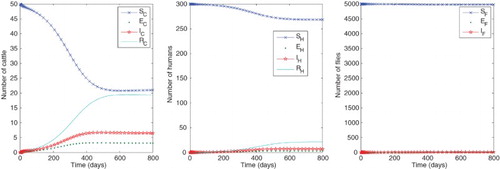
Figure 3. Numbers of humans, cattle and flies in each compartment with baseline parameter values as in Table 1 except $a=\frac{0.25}{2}$ with $I_F\left(0\right)=1$, $N_H=300$, $N_C=50$, $L^{\ast }=4545$, giving approximate equilibrium values $S_C^{\ast }=21,E_C^{\ast }=3,I_C^{\ast }=7,R_C^{\ast }=19,S_H^{\ast }=269,E_H^{\ast }=3,I_H^{\ast }=7,R_H^{\ast }=21,S_F^{\ast }=4979,E_F^{\ast }=9,I_F^{\ast }=12$. For these parameter values, the reproduction numbers are ${\mathcal{R}}_0=1.5149,{\mathcal{R}}_{0H}=0.9526,{\mathcal{R}}_{0C}=2.1253$.

5. Concluding remarks

This study provides a rigorous derivation of the basic reproduction ${\mathcal{R}}_0$ for our model of HAT transmission between tsetse flies, human and cattle hosts. By using a Lyapunov function, we prove that for ${\mathcal{R}}_0<1$, the DFE is globally asymptotically stable, thus HAT dies out; whereas for ${\mathcal{R}}_0>1$, the disease persists in all the populations. Under the assumption that HAT confers permanent immunity upon recovery, or that a host remains in stage II of the disease or in treatment for their entire lifetime (i.e. ${\kappa }_C={\kappa }_H=0$), we further prove the existence of a unique endemic equilibrium that is globally asymptotically stable in the interior of the invariant region. Using parameter values appropriate for HAT in Central Africa (mostly gleaned from the literature), we calculate elasticity indices for ${\mathcal{R}}_0$ with respect to different model parameters. Based on our numerical elasticity indices, ${\mathcal{R}}_0$ is very sensitive to pertubations in the fly blood feeding rate. It is also sensitive to cattle transmission parameters but less sensitive to human transmission parameters.

We note that, from our simulations at baseline parameter values, the number of infectious humans is about $10\mathrm{\%}$ of the population at equilibrium; this is higher than suggested by available data, for example, 7% [21] or 1–2 % [12, 20]. Treatment with drugs for the first and second stage of HAT is available, but we have only included treatment at the beginning of stage II. Our model does not distinguish between hosts in stage II of HAT, those under treatment and those recovered. In addition, our model ignores human and cattle death due to HAT, whereas if untreated and allowed to progress to the second stage, HAT is usually fatal. Further consideration of treatment and death due to HAT should be incorporated in an extended model, and may help to reduce the simulated number of infectious hosts to observed values. However, our elasticity indices give an indication that HAT can be prevented by adequate control of the flies by reducing ${\mathcal{R}}_0$ below 1. In fact, vector control is now recognized as part of the field strategy to eliminate HAT caused by T. b. gambiense [27].

Acknowledgments

The authors are grateful to the office of Prof. Mamokgethi Phakeng, Vice-Principal: Research and Innovation, UNISA and DST/NRF SARChI Chair in Mathematical Models and Methods in Bioengineering and Biosciences, University of Pretoria; for the funding and sponsoring of the 1st Joint Unisa — UP Workshop on Theoretical and Mathematical Epidemiology, Science Campus, Florida, South Africa, 2–8 March 2014, where the work was initiated. The authors thank Zhisheng Shuai (University of Central Florida) for suggesting the Lyapunov function used in the proof of Theorem 4, and two anonymous reviewers for helpful comments.

Disclosure statement

No potential conflict of interest was reported by the authors.

Additional information

Funding

The research of P.vdD. is partially supported by an NSERC Discovery grant, and the research of C.M.S.-R. is supported by NSERC through a USRA.

Appendix. Proof of Theorem 4

Consider $V_H=S_H-S_H^{\ast }-S_H^{\ast }\ln \frac{S_H}{S_H^{\ast }}+E_H-E_H^{\ast }-E_H^{\ast }\ln \frac{E_H}{E_H^{\ast }}+\frac{{\tilde{q}}_H}{q_H}\left(I_H-I_H^{\ast }-I_H^{\ast }\ln \frac{I_H}{I_H^{\ast }}\right).$Differentiating along solutions, using (16(16) $\frac{\mathrm{d}{E}_H}{\mathrm{d}}t=(1-p)ab{\frac{I_F{N}_H}{S}}_H-{\tilde{q}}_H{E}_H,$(16) ), (17(17) $\frac{\mathrm{d}{I}_H}{\mathrm{d}t}=q_H{E}_H-{\tilde{\gamma }}_H{I}_{H,}$(17) ), (23(23) $\frac{\mathrm{d}{R}_H}{\mathrm{d}t}={\gamma }_H{I}_H-(b_H+{\kappa }_H)R_H,$(23) ) with ${\kappa }_H=0$, substituting $b_H{N}_H=(1-p)\mathit{\text{ab}}\left(I_F^{\ast }/N_H\right)S_H^{\ast }+b_H{S}_H^{\ast }$ and ${\tilde{\gamma }}_H{I}_H^{\ast }=q_H{E}_H^{\ast }$ gives $\begin{array}{rl}{\dot{V}}_H& =b_H{S}_H^{\ast }\left(2-\frac{S_H}{S_H^{\ast }}-\frac{S_H^{\ast }}{S_H}\right)+(1-p)\mathit{\text{ab}}\left(\frac{I_F^{\ast }{S}_H^{\ast }}{N_H}-\frac{I_F^{\ast }}{N_H}\frac{S_H^{\ast 2}}{S_H}+\frac{I_F{S}_H^{\ast }}{N_H}-\frac{E_H^{\ast }}{E_H}\frac{I_F{S}_H}{N_H}\right)\\ & +{\tilde{q}}_H{E}_H^{\ast }\left(2-\frac{I_H}{I_H^{\ast }}-\frac{E_H}{E_H^{\ast }}\frac{I_H^{\ast }}{I_H}\right).\end{array}$Note that $2-x-1/x\le 0$ for x>0 with equality if and only if x=1, thus the first bracket in ${\dot{V}}_H$ is nonpositive. For the last bracket, (16(16) $\frac{\mathrm{d}{E}_H}{\mathrm{d}}t=(1-p)ab{\frac{I_F{N}_H}{S}}_H-{\tilde{q}}_H{E}_H,$(16) ) gives ${\tilde{q}}_H{E}_H^{\ast }=(1-p)\mathit{\text{ab}}{\mathrm{I}}_F^{\ast }{S}_H^{\ast }/N_H$. Using this ${\dot{V}}_H\le (1-p)\mathit{\text{ab}}\frac{I_F^{\ast }{S}_H^{\ast }}{N_H}\left(3-\frac{S_H^{\ast }}{S_H}+\frac{I_F}{I_F^{\ast }}-\frac{I_F}{I_F^{\ast }}\frac{E_H^{\ast }}{E_H}\frac{S_H}{S_H^{\ast }}-\frac{I_H}{I_H^{\ast }}-\frac{E_H}{E_H^{\ast }}\frac{I_H^{\ast }}{I_H}\right).$Similarly, defining $V_C=S_C-S_C^{\ast }-S_C^{\ast }\ln \frac{S_C}{S_C^{\ast }}+E_C-E_C^{\ast }-E_C^{\ast }\ln \frac{E_C}{E_C^{\ast }}+\frac{{\tilde{q}}_C}{q_C}\left(I_C-I_C^{\ast }-I_C^{\ast }\ln \frac{I_C}{I_C^{\ast }}\right).$differentiating along solutions, simplifying as above using (18(18) $\frac{\mathrm{d}{E}_C}{\mathrm{d}t}=\mathit{\text{pau}}\frac{I_F}{N_C}{S}_C-{\tilde{q}}_C{E}_C,$(18) )–(20(20) $\frac{\mathrm{d}{S}_F}{\mathrm{d}t}={\sigma }_L{L}^{\ast }-d_F{S}_F-(1-p)ac\frac{I_H}{N_H}{S}_F-\mathit{\text{pav}}\frac{I_C}{N_C}{S}_F,$(20) ) with ${\kappa }_C=0$ and ${\tilde{q}}_C{E}_C^{\ast }=\mathit{\text{pau}}\left(I_F^{\ast }/N_C\right)S_C^{\ast }$ gives ${\dot{V}}_C\le \mathit{\text{pau}}\frac{I_F^{\ast }{S}_C^{\ast }}{N_C}\left(3-\frac{S_C^{\ast }}{S_C}+\frac{I_F}{I_F^{\ast }}-\frac{I_F}{I_F^{\ast }}\frac{S_C}{S_C^{\ast }}\frac{E_C^{\ast }}{E_C}-\frac{I_C}{I_C^{\ast }}-\frac{E_C}{E_C^{\ast }}\frac{I_C^{\ast }}{I_C}\right).$Similarly, defining $V_F=S_F-S_F^{\ast }-S_F^{\ast }\ln \frac{S_F}{S_F^{\ast }}+E_F-E_F^{\ast }-E_F^{\ast }\ln \frac{E_F}{E_F^{\ast }}+\frac{{\tilde{q}}_F}{q_F}\left(I_F-I_F^{\ast }-I_F^{\ast }\ln \frac{I_F}{I_F^{\ast }}\right),$differentiating along solutions and simplifying as above, gives $\begin{array}{rl}{\dot{V}}_F& \le (1-p)\mathit{\text{ac}}\frac{I_H^{\ast }{S}_F^{\ast }}{N_H}\left(3-\frac{S_F^{\ast }}{S_F}-\frac{I_F}{I_F^{\ast }}-\frac{I_F^{\ast }}{I_F}\frac{E_F}{E_F^{\ast }}+\frac{I_H}{I_H^{\ast }}-\frac{I_H}{I_H^{\ast }}\frac{S_F}{S_F^{\ast }}\frac{E_F^{\ast }}{E_F}\right)\\ & +\mathit{\text{pav}}\frac{I_C^{\ast }{S}_F^{\ast }}{N_C}\left(3-\frac{I_F}{I_F^{\ast }}-\frac{I_F^{\ast }}{I_F}\frac{E_F}{E_F^{\ast }}-\frac{S_F^{\ast }}{S_F}+\frac{I_C}{I_C^{\ast }}-\frac{I_C}{I_C^{\ast }}\frac{S_F}{S_F^{\ast }}\frac{E_F^{\ast }}{E_F}\right).\end{array}$

Now, consider the linear combination $V_{FHC}=\left(c{I}_H^{\ast }{S}_F^{\ast }/b{I}_F^{\ast }{S}_H^{\ast }\right)V_H+\left(v{I}_C^{\ast }{S}_F^{\ast }/u{I}_F^{\ast }{S}_C^{\ast }\right)V_C+V_F$, where the constants can be found from the graphical approach in [24]. This gives $\begin{array}{rl}{\dot{V}}_{FHC}& \le (1-p)\mathit{\text{ac}}\frac{I_H^{\ast }{S}_F^{\ast }}{N_H}\left(6-\frac{S_H^{\ast }}{S_H}-\frac{S_F^{\ast }}{S_F}-\frac{I_F}{I_F^{\ast }}\frac{S_H}{S_H^{\ast }}\frac{E_H^{\ast }}{E_H}-\frac{E_H}{E_H^{\ast }}\frac{I_H^{\ast }}{I_H}-\frac{I_H}{I_H^{\ast }}\frac{S_F}{S_F^{\ast }}\frac{E_F^{\ast }}{E_F}-\frac{E_F}{E_F^{\ast }}\frac{I_F^{\ast }}{I_F}\right)\\ & +\mathit{\text{pav}}\frac{I_C^{\ast }{S}_F^{\ast }}{N_C}\left(6-\frac{S_C^{\ast }}{S_C}-\frac{S_F^{\ast }}{S_F}-\frac{I_F}{I_F^{\ast }}\frac{S_C}{S_C^{\ast }}\frac{E_C^{\ast }}{E_C}-\frac{E_C}{E_C^{\ast }}\frac{I_C^{\ast }}{I_C}-\frac{I_C}{I_C^{\ast }}\frac{S_F}{S_F^{\ast }}\frac{E_F^{\ast }}{E_F}-\frac{E_F}{E_F^{\ast }}\frac{I_F^{\ast }}{I_F}\right).\end{array}$The terms in the first bracket above can be written as $\begin{array}{rl}& 1-\frac{S_H^{\ast }}{S_H}+\ln \frac{S_H^{\ast }}{S_H}+1-\frac{S_F^{\ast }}{S_F}+\ln \frac{S_F^{\ast }}{S_F}+1-\frac{I_F{S}_H{E}_H^{\ast }}{I_F^{\ast }{S}_H^{\ast }{E}_H}+\ln \frac{I_F{S}_H{E}_H^{\ast }}{I_F^{\ast }{S}_H^{\ast }{E}_H}\\ & +1-\frac{E_H{I}_H^{\ast }}{E_H^{\ast }{I}_H}+\ln \frac{E_H{I}_H^{\ast }}{E_H^{\ast }{I}_H}+1-\frac{I_H{S}_F{E}_F^{\ast }}{I_H^{\ast }{S}_F^{\ast }{E}_F}+\ln \frac{I_H{S}_F{E}_F^{\ast }}{I_H^{\ast }{S}_F^{\ast }{E}_F}+1-\frac{E_F{I}_F^{\ast }}{E_F^{\ast }{I}_F}+\ln \frac{E_F{I}_F^{\ast }}{E_F^{\ast }{I}_F}.\end{array}$since the ln terms cancel. Noting that $1-x+\ln x\le 0$ for x>0 with equality if and only if x=1. Similarly rewriting the terms in the second bracket, shows that ${\dot{V}}_{FHC}\le 0$. Also considering the case of equality, it can be seen that ${\dot{V}}_{FHC}=0$ if and only if $(E_F,I_F,E_H,I_H,E_C,I_C,S_F,S_H)=(E_F^{\ast },I_F^{\ast },E_H^{\ast },I_H^{\ast },E_C^{\ast },I_C^{\ast },S_F^{\ast },S_H^{\ast })$.

Thus $V_{FHC}$ is a Lyapunov function, proving uniqueness and global asymptotic stability of $X^{\ast }$ in $\mathrm{int}\left(\mathrm{\Gamma }\right)$ provided that ${\mathcal{R}}_0>1$ and ${\kappa }_H={\kappa }_C=0$.

References

- R.M. Anderson and R.M. May, Infectious Diseases of Humans: Dynamics and Control, Oxford University Press, Oxford, 1991.
- M. Artzrouni and J.-P. Gouteux, Control strategies for sleeping sickness in Central Africa: a model-based approach, Trop. Med. Int. Health 1(6) (1996), pp. 753–764.
- M. Artzrouni and J.-P. Gouteux, A compartmental model of sleeping sickness in central Africa, J. Biol. Syst. 4(4) (1996), pp. 459–477.
- D. Bruce, Preliminary Report on the Tsetse Fly Disease Or Nagana, in Zululand, Bennett & Davis, Durban, 1895.
- D. Bruce, A. E. Hamerton, H.R. Bateman, and F.P. Mackie, The development of Trypanosoma gambiense in Glossina palpalis, Proc. R. Soc. B: Biol. Sci. 81(550) (1909), pp. 405–414.
- A. Castellani, On the discovery of a species of trypanosoma in the cerebrospinal fluid of cases of sleeping sickness, The Lancet 161(4164) (1903), pp. 1735–1736.
- K. Chalvet-Monfray, M. Artzrouni, J.-P. Gouteux, P. Auger, and P. Sabatier, A two-patch model of Gambian sleeping sickness: application to vector control strategies in a village and plantations, Acta Biotheor. 46(3) (1998), pp. 207–222.
- S. Davis, S. Aksoy, and A. Galvani, A global sensitivity analysis for African sleeping sickness, Parasitology 138 (2011), pp. 516–526.
- L. Edelstein-Keshet, Mathematical Models in Biology, McGraw-Hill, New York, 1988 (reprinted by SIAM, Philadelphia, 2003).
- J.R. Franco, P.P. Simarro, A. Diarra, and J.G. Jannin, Epidemiology of human African trypanosomiasis, Clinical Epidemiology 6 (2014), pp. 257–275.
- H.I. Freedman, S. Ruan, and M. Tang, Uniform persistence and flows near a closed positively invariant set, J. Dyn. Differ. Eq. 6(4) (1994), pp. 583–600.
- S. Funk, H. Nishiura, H. Heesterbeek, W. John Edmunds, and F. Checchi, Identifying transmission cycles at the human-animal interface: the role of animal reservoirs in maintaining gambiense human African trypanosomiasis, PLoS Comput. Biol. 9(1) (2013).
- J.W. Hargrove, R. Ouifki, D. Kajunguri, G.A. Vale, and S.J. Torr, Modeling the control of trypanosomiasis using trypanocides or insecticide-treated livestock, PLoS Negl. Trop. Dis. 6 (5)(2012), p. e1615.
- D. Kajunguri, J.W. Hargrove, R. Oufki, J.Y.T. Mugisha, P.G. Coleman, and S.C. Welburn, Modelling the use of insecticide-treated cattle to control tsetse and Trypanosoma brucei rhodiense in a multi-host population, Bull. Math. Biol. 76 (2014), pp. 673–696.
- M.Y. Li, J.R. Graef, L. Wang, and J. Karsai, Global dynamics of a SEIR model with varying total population size, Math. Biosci. 160 (1999), pp. 191–213.
- A.K. Lindner and G. Priotto, The unknown risk of vertical transmission in sleeping sickness – a literature review, PLoS Negl. Trop. Dis. 4(12) (2010), p. e783.
- G. MacDonald, The Epidemiology and Control of Malaria, Oxford University Press, Oxford, 1957.
- T. Madsen, D.I. Wallace, and N. Zupan, Seasonal fluctuation in tsetse fly populations and human African trypanosomiasis: a mathematical model, BIOMAT 2012 (2013), pp. 56–69.
- D. Moulay, M.A. Aziz-Alaoui, and M. Cadivel, The chikungunya disease: modeling, vector and transmission global dynamics, Math. Biosci. 229(1) (2011), pp. 50–63.
- K.S. Rock, C.M. Stone, I.M. Hastings, M.J. Keeling, S.J. Torr, and N. Chitnis, Mathematical models of human African trypanosomiasis epidemiology, Adv. Parasitol. 87 (2015).
- D.J. Rogers, A general model for the African trypanosomiases, Parasitology 97(Pt 1) (1988), pp. 193–212.
- R. Ross, The Mathematics of Malaria, Vol. 1, 2nd ed., Murray, London, 1911.
- J.A. Rozendaal, Vector control: methods for use by individuals and communities, Tech. Rep., Geneva, 1997.
- Z. Shuai and P. van den Driessche, Global stability of infectious disease models using Lyapunov functions, SIAM J. Appl. Math. 73(4) (2013), pp. 1513–1532.
- P.P. Simarro, J.R. Franco, A. Diarra, J.A. Ruiz Postigo, and J. Jannin, Diversity of human African trypanosomiasis epidemiological settings requires fine-tuning control strategies to facilitate disease elimination, Res. Rep. Trop. Med. 4 (2013), pp. 1–6.
- H.L. Smith and P. Waltman, The Theory of the Chemostat: Dynamics of Microbial Competition, Cambridge University Press, Cambridge, 1995.
- P. Solano, S.J. Torr, and M.J. Lehane, Is vector control needed to eliminate gambiense human african trypanosomiasis?, Front. Cell. Infect. Microbiol. 3(33) (2013).
- P. Steinmann, C.M. Stone, C. Simone Sutherland, M. Tanner, and F. Tediosi, Contemporary and emerging strategies for eliminating human African trypanosomiasis due to Trypanosoma brucei gambiense: review, Trop. Med. Int. Health 20(6) (2015), pp. 707–718.
- P. van den Driessche and J. Watmough, Reproduction numbers and sub-threshold endemic equilibria for compartmental models of disease transmission, Math. Biosci. 180 (2002), pp. 29–48.