Optimal insecticide-treated bed-net coverage and malaria treatment in a malaria-HIV co-infection model

ABSTRACT

We propose and study a mathematical model for malaria-HIV co-infection transmission and control, in which malaria treatment and insecticide-treated nets are incorporated. The existence of a backward bifurcation is established analytically, and the occurrence of such backward bifurcation is influenced by disease-induced mortality, insecticide-treated bed-net coverage and malaria treatment parameters. To further assess the impact of malaria treatment and insecticide-treated bed-net coverage, we formulate an optimal control problem with malaria treatment and insecticide-treated nets as control functions. Using reasonable parameter values, numerical simulations of the optimal control suggest the possibility of eliminating malaria and reducing HIV prevalence significantly, within a short time horizon.

KEYWORDS:

• Malaria-HIV co-infection
• malaria control
• insecticide-treated nets
• treatment
• optimalcontrol

AMS SUBJECT CLASSIFICATION:

• 49J15
• 92B05

1. Introduction

Malaria and HIV are among the deadliest diseases of our time and they cause 4 million deaths a year [2]. Both malaria and HIV are endemic in sub-Saharan regions of Africa, in some parts of Asia and Latin America. The wide geographic overlap in occurrence of these diseases facilitates co-infection, and the interaction between the two diseases clearly has major public health implications [2, 17]. There is growing evidence that the two infections may simultaneously intensify each other, resulting in an increase in incidence and complication in treatment efforts; and therefore understanding the impact of malaria and HIV co-infection, and designing effective control strategies are important [31].

Malaria is a deadly infectious disease caused by a parasite called Plasmodium, which is transmitted to humans via bites by infected female mosquitoes. Female mosquitoes require blood meals to produce eggs and only anopheles mosquitoes transmit malaria. In order to transmit the disease, a female anopheles mosquito must have been infected in a previous blood meal from an infected person [15, 18, 24]. The disease remains a major burden in many parts of the world, with Africa and south-east Asia at high risk of malaria infection [36]. According to the latest estimate released by WHO in December 2014, there were about 198 million cases of malaria in 2013 and an estimated 584,000 deaths, of which 437,000 of these were children under the age of five [36]. Globally, the number of malaria cases decreased since 2000. However, malaria is still of public health concern, with high mortality in children [36]. There is a wide range of malaria intervention strategies, some of which are: insecticide-treated nets [1, 24], indoor residual spraying [34,  36], anti-malarial drugs such as artemesinin combination therapy [32,  36], and intermittent preventive treatment in children (IPTi) and in pregnant women (IPTp) [32]. Several studies have been conducted to investigate the efficacy and efficiency of these interventions as well as how best to integrate these control efforts in a fight against malaria (see [3, 15, 18, 24, 32, 34] and references therein).

HIV, which stands for human immunodeficiency virus, is one of the leading causes of death worldwide, affecting mostly impoverished people in sub-Sahara Africa [17]. The virus attacks the immune system and weakens individual's defence systems against infections and some types of cancer. HIV can be transmitted via the exchange of a variety of body fluids from infected individuals, such as blood, breast milk, semen and vaginal secretions. The most advanced stage of HIV infection is Acquired Immunodeficiency Syndrome (AIDS), which can take from 2 to 15 years to develop depending on the individual's immune system. There have been 39 million HIV-related deaths worldwide since the 1980s, with 1.5 million in 2013 alone, and out of approximately 35 million people living with HIV worldwide, 24.7 million people are in sub-Saharan Africa [35]. Also, 2.1 million people became newly infected globally in 2013; sub-Saharan Africa accounts for almost 70% of the global total of new HIV infections [35]. Even though there is no cure for HIV infection, effective treatment with anti-retroviral (ARV) drugs is important in controlling the virus so that people with HIV can live longer. However, in impoverished countries where HIV is most widespread, there are several obstacles to providing efficient treatment, some of which are: insufficient medical facilities and the high cost of drugs relative to local incomes or government health budgets.

Malaria and HIV overlap geographically in sub-Saharan Africa, South-east Asia and South America; both diseases are endemic and have devastating effects on people living in these endemic areas [2]. The geographical overlap of the two infections has generated global interest to understand their potential interactions and to develop effective integrated disease control strategies [19, 29]. HIV infection can increase the risk and severity of malaria infection and the increased parasite burdens might increase transmission (the impact of malaria disease and death). Individuals in malaria endemic areas that are considered semi-immune to malaria can also develop clinical malaria if they are infected with HIV. Recent study from east sub-Saharan Africa indicated malaria as a risk factor of concurrent HIV infection at the population level [29]. On the other hand, for individuals infected with HIV, the presence of malaria infection tends to increase HIV viral load, and consequently, HIV replication [2,  17].

Few population-based studies with mathematical models are available to determine the number of patients affected by co-infection and the impact of co-infection on a population [17, 23]. Barely et al. [17] proposed a mathematical model to study the effect of HIV-Malaria co-infection in a simple setting and carried out sensitivity analysis using data collected from Malawi. Mukandavire et al. [23] utilized a mathematical analysis of a comprehensive model to study transmission dynamics of HIV and malaria and found out that HIV-induced increase in susceptibility to malaria infection has marginal effect on the number of new cases of HIV, but significantly increases the number of new cases of malaria-HIV co-infection. Recently, Nyabadza et al. [25] proposed a mathematical model for HIV-malaria co-infection and investigated the role of HIV treatment on the dynamics of malaria. Their results demonstrate that malaria-HIV co-infection amplify HIV/AIDS prevalence and HIV treatment helps to mitigate the harmful effects of malaria-HIV co-infection, especially for AIDS infected patients. Cuadros et al. [10] developed and analysed a stochastic, individual-based, co-infection model that incorporates the dynamics of HIV and the co-infection effect on the HIV transmission caused by other infectious diseases such as malaria, gonorrhea and syphilis. Simulation result shows that an epidemic can be generated as a result of amplification effect caused by the co-infection, and without amplification effect, no epidemic is generated. The amplification effect is due to an increase on HIV viral load caused by the co-infection, which amplify the risk of HIV transmission [10]. Also, a similar work in [9] found that the amplification effect caused by malaria-HIV co-infection is responsible for maintaining HIV in sub-Saharan Africa.

In our work, we propose and study a mathematical model for malaria-HIV co-infection transmission and control, in which insecticide-treated nets and malaria treatment are incorporated. An optimal control problem which seeks to minimize the number of humans infected with malaria, co-infected with malaria and HIV, the number of infected mosquitoes, and the cost of implementing insecticide-treated nets and malaria treatment control strategies is formulated. Similar models have been studied, for example, the models in [23, 25]. However, our model is different in that it incorporates bed-net and treatment controls in a susceptible-infectious-recovered-susceptible (SIRS) model for malaria in humans, susceptible-infectious (SI) model for HIV and SI model for the mosquito population; also, optimal control strategies are investigated with these control actions as control functions.

The remainder of the paper is organized as follows: in Section 2, the co-infection model is formulated, in Section 3 stability analysis and corresponding numerical results are presented and discussed. The optimal control problem is formulated and analysed, and corresponding numerical simulations are presented in Section 4. Concluding remarks and discussions are presented in Section 5.

2. Model derivation

We divide the total human population, N, into six different classes: $S,I_m,R_m,I_h,I_{hm}$ and $R_{hm}$. S represents the susceptible class; $I_m$ represents malaria infectious class; $R_m$ represents the recovered temporary immune (to malaria) class, $I_h$ represents HIV-infectious class; $I_{hm}$ represents the class of infectious individuals co-infected with both HIV and malaria and $R_{hm}$ represents recovered temporary immune (to malaria), but HIV-infectious class. The total mosquito population, $N_v$, is divided into two classes, $S_v$ and $I_v$, of susceptible mosquitoes and infectious mosquitoes, respectively.

We assume that newly recruited humans are susceptible and are recruited at rate ${\mathrm{\Lambda }}_h$. Susceptible humans acquire malaria at rate ${\lambda }_h$ (defined in (4(4) ${\lambda }_h=\frac{p_{vh}\beta \left(b\right)I_v}{N},{\lambda }_v^m=\frac{p_{hv}\beta \left(b\right)I_m}{N},\text{and}{\lambda }_v^{hm}=\frac{p_{hv}\beta \left(b\right)I_{hm}}{N},$(4) )) after being bitten by an infected mosquito, and progress to the malaria infectious class. Humans in $I_m$ class receive treatment at rate u. After treatment, a proportion, σ, of those who recover from malaria infection without immunity returns to the S class, and the proportion, $(1-\sigma )$, who recover with temporary immunity to malaria progresses to the recovered class, $R_m$. We also assume that humans in the $I_m$ class acquire temporary immunity, and recover naturally at rate γ to join the $R_m$ class. Individuals in the $R_m$ class lose their temporary immunity at rate ρ and become susceptible to malaria. Humans in the $I_m$ class suffer malaria-induced mortality at rate ${\mu }_m$.

We assume that susceptible humans cannot be infected simultaneously with malaria and HIV, since the transmission mechanism for the two diseases are completely different. To enter the $I_{hm}$ class, an individual must be infected with HIV (i.e. $I_h$) or malaria (i.e. $I_m$) prior to infection with the other disease. An individual or human in the $I_{hm}$ class transmits both diseases, and since the individual's immune system is compromised, the transmission probability is higher given a contact has occurred, whereby a contact we mean any process that results in transmission of HIV infection. Also, when humans in the $I_m$ class are infected with HIV, they progress to the $I_{hm}$ class at rate ${\omega }_h$ if contact occurred with a person in the $I_h$ or in the $R_{hm}$ class at rate ${\alpha }_2{\omega }_{hm}$ if contact occurred with a person in the $I_{hm}$ class (both ${\omega }_h$ and ${\omega }_{hm}$ are the forces of infection for HIV, and are defined in (5(5) ${\omega }_h=\frac{{\beta }_h(I_h+R_{hm})}{N}\text{and}{\omega }_{hm}=\frac{{\beta }_h{I}_{hm}}{N}.$(5) )). The constant ${\alpha }_2>1$ is an amplification factor that captures the fact that individuals co-infected with both diseases are highly infectious. When susceptible humans are infected with HIV, they progress to the $I_h$ class at rate ${\omega }_h$ if the contact is with humans in the $I_h$ or in the $R_{hm}$ class at rate ${\alpha }_1{\omega }_{hm}$ if contact occurred with individuals in the $I_{hm}$ class. The constant ${\alpha }_1>1$ is also an amplification factor. Also, when individuals in $R_m$ class are infected with HIV, they join the $R_{hm}$ class at rate ${\omega }_h$ when contact is with individuals in the $I_h$ or $R_{hm}$ class, and at rate ${\alpha }_1{\omega }_{hm}$ when contact is with individuals in the $I_{hm}$ class. When individuals in $I_{hm}$ receive malaria treatment at rate u, a proportion, σ, of them recover from malaria without immunity and join the $I_h$ class, and the rest who recover with temporary immunity to malaria join the $R_{hm}$ class.

Individuals in $I_{hm}$ class recover with temporary immunity to malaria and progress to the $R_{hm}$ class at rate ${\kappa }_1\gamma$, and individuals in $R_{hm}$ class lose temporary immunity to malaria and join the $I_h$ class at rate ${\kappa }_2\rho$. The constants ${\kappa }_1<1$ and ${\kappa }_2>1$ capture the fact that the immune system of HIV-infected individuals is compromised [17]. When individuals in $I_h$ class are infected with malaria, they move to the $I_{hm}$ class at rate ${\alpha }_3{\lambda }_h$, where the constant ${\alpha }_3>1$ is an amplification factor. Individuals in $I_h$ and $R_{hm}$ classes suffer disease-induced mortality at rate ${\mu }_h$, and individuals in $I_{hm}$ class suffers disease-induced mortality at rate ${\mu }_{hm}$. The natural mortality rate for all humans is μ.

Mosquitoes are recruited at a constant rate ${\mathrm{\Lambda }}_v$ and newly recruited mosquitoes are assumed to be susceptible. Susceptible mosquitoes are infected with malaria at rate ${\lambda }_v^m$ when they bite a malaria-infected human, and at rate ${\alpha }_4{\lambda }_v^{hm}$ when they bite an individual co-infected with malaria and HIV. The constant ${\alpha }_4>1$ is an amplification factor, since individuals in $I_{hm}$ class are highly infectious. The amplification constants, ${\alpha }_i,i=1,2,3,4$, are discussed in detail in [17], and ${\lambda }_v^m$ and ${\lambda }_v^{hm}$ are defined in (4(4) ${\lambda }_h=\frac{p_{vh}\beta \left(b\right)I_v}{N},{\lambda }_v^m=\frac{p_{hv}\beta \left(b\right)I_m}{N},\text{and}{\lambda }_v^{hm}=\frac{p_{hv}\beta \left(b\right)I_{hm}}{N},$(4) ). All mosquitoes suffer mortality at a rate of ${\mu }_v\left(b\right)$, where ${\mu }_v\left(b\right)$ is defined in (3(3) ${\mu }_v\left(b\right)={\mu }_{v0}+{\mu }_{v1}b,$(3) ).

See Table 1 for a brief description and baseline values of parameters used in the model, and Figure 1 for schematics of the model.

Figure 1. Schematics model diagram.

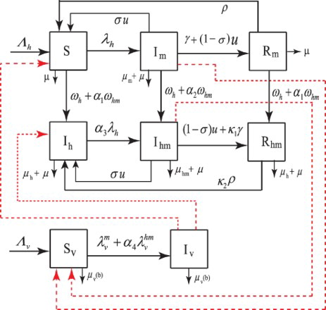
From the above description, the model that governs the transmission of the malaria and HIV is: (1) $\begin{array}{rl}\dot{S}& ={\mathrm{\Lambda }}_h+\sigma u{I}_m+\rho R_m-({\lambda }_h+{\omega }_h+{\alpha }_1{\omega }_{hm}+\mu )S\\ {\dot{I}}_m& ={\lambda }_{h}S-({\omega }_h+{\alpha }_2{\omega }_{hm}+\gamma +u+{\mu }_m+\mu )I_m\\ {\dot{R}}_m& =(\gamma +(1-\sigma \left)u\right)I_m-({\omega }_h+{\alpha }_1{\omega }_{hm}+\rho +\mu )R_m\\ {\dot{I}}_{hm}& =({\omega }_h+{\alpha }_2{\omega }_{hm})I_m+{\alpha }_3{\lambda }_h{I}_h-({\kappa }_1\gamma +u+{\mu }_{hm}+\mu )I_{hm}\\ {\dot{R}}_{hm}& =\left(\right(1-\sigma )u+{\kappa }_1\gamma )I_{hm}+({\omega }_h+{\alpha }_1{\omega }_{hm})R_m-({\kappa }_2\rho +{\mu }_h+\mu )R_{hm}\\ {\dot{I}}_h& =\sigma u{I}_{hm}+{\kappa }_2\rho R_{hm}+({\omega }_h+{\alpha }_1{\omega }_{hm})S-({\alpha }_3{\lambda }_h+{\mu }_h+\mu )I_h\\ {\dot{S}}_v& ={\mathrm{\Lambda }}_v-({\lambda }_v^m+{\alpha }_4{\lambda }_v^{hm}+{\mu }_v(b\left)\right)S_v\\ {\dot{I}}_v& =({\lambda }_v^m+{\alpha }_4{\lambda }_v^{hm})S_v-{\mu }_v\left(b\right)I_v,\end{array}$(1) where the respective total human and mosquito populations are governed by the equations (2) ${\dot{N}}_h={\mathrm{\Lambda }}_h-{\mu }_h{N}_h-{\mu }_m{I}_m-{\mu }_{hm}{I}_{hm}-{\mu }_h(R_{hm}+I_h);{\dot{N}}_v={\mathrm{\Lambda }}_v-{\mu }_v\left(b\right)N_v.$(2) As in [1], the biting or contact rate of mosquitoes, $\beta \left(b\right)$, is defined by $\beta \left(b\right)={\beta }_{\max }-({\beta }_{\max }-{\beta }_{\min })b,$ where ${\beta }_{min}$ is the minimum mosquito biting rate, ${\beta }_{max}$ is the maximum mosquito biting rate and b is insecticide bed-net coverage. Due to insecticide treatment of bed nets, female mosquitoes questing for blood meal could die when they come in contact with a treated bed net. As in [1], we have modelled mosquito death rate as: (3) ${\mu }_v\left(b\right)={\mu }_{v0}+{\mu }_{v1}b,$(3) where ${\mu }_{v0}$ is mosquito natural death rate and ${\mu }_{v1}>0$ is the additional mortality due to treated insecticide bed-net usage. The forces of infection for malaria are defined by: (4) ${\lambda }_h=\frac{p_{vh}\beta \left(b\right)I_v}{N},{\lambda }_v^m=\frac{p_{hv}\beta \left(b\right)I_m}{N},\text{and}{\lambda }_v^{hm}=\frac{p_{hv}\beta \left(b\right)I_{hm}}{N},$(4) where $p_{vh}$ is the probability of disease transmission from infectious mosquitoes to susceptible humans, and $p_{hv}$ is the probability of disease transmission from infectious humans to susceptible mosquitoes. Similarly, the forces of infection for HIV are defined by: (5) ${\omega }_h=\frac{{\beta }_h(I_h+R_{hm})}{N}\text{and}{\omega }_{hm}=\frac{{\beta }_h{I}_{hm}}{N}.$(5)

3. Analysis and stability of the model

3.1. Local stability of the disease-free equilibrium

We set $K_0=\gamma +u+{\mu }_m+\mu$, $K_1=\gamma +(1-\sigma )u$, $K_2=\rho +\mu$, $K_3={\kappa }_1\gamma +u+{\mu }_{hm}+\mu$, $K_4=(1-\sigma )u+{\kappa }_1\gamma$, $K_5={\kappa }_2\rho +{\mu }_h+\mu$, and $K_6={\mu }_h+\mu$, for convenience, and define the biological feasible region ${\mathbb{D}}_{hm}\subset {\mathbb{R}}^8$, where (6) ${\mathbb{D}}_{hm}=\left\{(S,I_m,R_m,I_{hm},R_{hm},I_h,S_v,I_v)\in {\mathbb{R}}^8:0<N\le \frac{{\mathrm{\Lambda }}_h}{\mu },0<N_v\le \frac{{\mathrm{\Lambda }}_v}{{\mu }_v\left(b\right)}\right\},$(6) is positively invariant and attracting for the system (1(1) $\begin{array}{rl}\dot{S}& ={\mathrm{\Lambda }}_h+\sigma u{I}_m+\rho R_m-({\lambda }_h+{\omega }_h+{\alpha }_1{\omega }_{hm}+\mu )S\\ {\dot{I}}_m& ={\lambda }_{h}S-({\omega }_h+{\alpha }_2{\omega }_{hm}+\gamma +u+{\mu }_m+\mu )I_m\\ {\dot{R}}_m& =(\gamma +(1-\sigma \left)u\right)I_m-({\omega }_h+{\alpha }_1{\omega }_{hm}+\rho +\mu )R_m\\ {\dot{I}}_{hm}& =({\omega }_h+{\alpha }_2{\omega }_{hm})I_m+{\alpha }_3{\lambda }_h{I}_h-({\kappa }_1\gamma +u+{\mu }_{hm}+\mu )I_{hm}\\ {\dot{R}}_{hm}& =\left(\right(1-\sigma )u+{\kappa }_1\gamma )I_{hm}+({\omega }_h+{\alpha }_1{\omega }_{hm})R_m-({\kappa }_2\rho +{\mu }_h+\mu )R_{hm}\\ {\dot{I}}_h& =\sigma u{I}_{hm}+{\kappa }_2\rho R_{hm}+({\omega }_h+{\alpha }_1{\omega }_{hm})S-({\alpha }_3{\lambda }_h+{\mu }_h+\mu )I_h\\ {\dot{S}}_v& ={\mathrm{\Lambda }}_v-({\lambda }_v^m+{\alpha }_4{\lambda }_v^{hm}+{\mu }_v(b\left)\right)S_v\\ {\dot{I}}_v& =({\lambda }_v^m+{\alpha }_4{\lambda }_v^{hm})S_v-{\mu }_v\left(b\right)I_v,\end{array}$(1) ). The disease-free equilibrium (DFE) $E_{df}$ is calculated by setting the infectious classes, $I_m,I_{hm},R_{hm},I_h$, and $I_v$, to zero. This yields: (7) $E_{df}=\left(\frac{{\mathrm{\Lambda }}_h}{\mu },0,0,0,0,0,\frac{{\mathrm{\Lambda }}_v}{{\mu }_v\left(b\right)},0\right).$(7) The next generation approach in [11] is used to calculate the basic reproduction number ${\mathcal{R}}_0$ for the model system (1(1) $\begin{array}{rl}\dot{S}& ={\mathrm{\Lambda }}_h+\sigma u{I}_m+\rho R_m-({\lambda }_h+{\omega }_h+{\alpha }_1{\omega }_{hm}+\mu )S\\ {\dot{I}}_m& ={\lambda }_{h}S-({\omega }_h+{\alpha }_2{\omega }_{hm}+\gamma +u+{\mu }_m+\mu )I_m\\ {\dot{R}}_m& =(\gamma +(1-\sigma \left)u\right)I_m-({\omega }_h+{\alpha }_1{\omega }_{hm}+\rho +\mu )R_m\\ {\dot{I}}_{hm}& =({\omega }_h+{\alpha }_2{\omega }_{hm})I_m+{\alpha }_3{\lambda }_h{I}_h-({\kappa }_1\gamma +u+{\mu }_{hm}+\mu )I_{hm}\\ {\dot{R}}_{hm}& =\left(\right(1-\sigma )u+{\kappa }_1\gamma )I_{hm}+({\omega }_h+{\alpha }_1{\omega }_{hm})R_m-({\kappa }_2\rho +{\mu }_h+\mu )R_{hm}\\ {\dot{I}}_h& =\sigma u{I}_{hm}+{\kappa }_2\rho R_{hm}+({\omega }_h+{\alpha }_1{\omega }_{hm})S-({\alpha }_3{\lambda }_h+{\mu }_h+\mu )I_h\\ {\dot{S}}_v& ={\mathrm{\Lambda }}_v-({\lambda }_v^m+{\alpha }_4{\lambda }_v^{hm}+{\mu }_v(b\left)\right)S_v\\ {\dot{I}}_v& =({\lambda }_v^m+{\alpha }_4{\lambda }_v^{hm})S_v-{\mu }_v\left(b\right)I_v,\end{array}$(1) ). This gives: (8) ${\mathcal{R}}_0=max\{{\mathcal{R}}_h,{\mathcal{R}}_m\}.$(8) where, (9) ${\mathcal{R}}_h=\frac{{\beta }_h}{{\mu }_h+\mu }\text{and}{\mathcal{R}}_m=\frac{\beta \left(b\right)}{{\mu }_v\left(b\right)}\sqrt{\frac{p_{hv}{p}_{vh}{\mathrm{\Lambda }}_v\mu }{{\mathrm{\Lambda }}_h(\gamma +u+{\mu }_m+\mu )}}.$(9) The threshold ${\mathcal{R}}_h$ is the basic reproduction number of the malaria-free sub-model obtained from model (1(1) $\begin{array}{rl}\dot{S}& ={\mathrm{\Lambda }}_h+\sigma u{I}_m+\rho R_m-({\lambda }_h+{\omega }_h+{\alpha }_1{\omega }_{hm}+\mu )S\\ {\dot{I}}_m& ={\lambda }_{h}S-({\omega }_h+{\alpha }_2{\omega }_{hm}+\gamma +u+{\mu }_m+\mu )I_m\\ {\dot{R}}_m& =(\gamma +(1-\sigma \left)u\right)I_m-({\omega }_h+{\alpha }_1{\omega }_{hm}+\rho +\mu )R_m\\ {\dot{I}}_{hm}& =({\omega }_h+{\alpha }_2{\omega }_{hm})I_m+{\alpha }_3{\lambda }_h{I}_h-({\kappa }_1\gamma +u+{\mu }_{hm}+\mu )I_{hm}\\ {\dot{R}}_{hm}& =\left(\right(1-\sigma )u+{\kappa }_1\gamma )I_{hm}+({\omega }_h+{\alpha }_1{\omega }_{hm})R_m-({\kappa }_2\rho +{\mu }_h+\mu )R_{hm}\\ {\dot{I}}_h& =\sigma u{I}_{hm}+{\kappa }_2\rho R_{hm}+({\omega }_h+{\alpha }_1{\omega }_{hm})S-({\alpha }_3{\lambda }_h+{\mu }_h+\mu )I_h\\ {\dot{S}}_v& ={\mathrm{\Lambda }}_v-({\lambda }_v^m+{\alpha }_4{\lambda }_v^{hm}+{\mu }_v(b\left)\right)S_v\\ {\dot{I}}_v& =({\lambda }_v^m+{\alpha }_4{\lambda }_v^{hm})S_v-{\mu }_v\left(b\right)I_v,\end{array}$(1) ) by setting $I_m=0$, $R_m=0$, $I_{hm}=0$ and $R_{hm}=0$, and the threshold ${\mathcal{R}}_m$ is the basic reproduction number of the HIV-free sub-model obtained from model (1(1) $\begin{array}{rl}\dot{S}& ={\mathrm{\Lambda }}_h+\sigma u{I}_m+\rho R_m-({\lambda }_h+{\omega }_h+{\alpha }_1{\omega }_{hm}+\mu )S\\ {\dot{I}}_m& ={\lambda }_{h}S-({\omega }_h+{\alpha }_2{\omega }_{hm}+\gamma +u+{\mu }_m+\mu )I_m\\ {\dot{R}}_m& =(\gamma +(1-\sigma \left)u\right)I_m-({\omega }_h+{\alpha }_1{\omega }_{hm}+\rho +\mu )R_m\\ {\dot{I}}_{hm}& =({\omega }_h+{\alpha }_2{\omega }_{hm})I_m+{\alpha }_3{\lambda }_h{I}_h-({\kappa }_1\gamma +u+{\mu }_{hm}+\mu )I_{hm}\\ {\dot{R}}_{hm}& =\left(\right(1-\sigma )u+{\kappa }_1\gamma )I_{hm}+({\omega }_h+{\alpha }_1{\omega }_{hm})R_m-({\kappa }_2\rho +{\mu }_h+\mu )R_{hm}\\ {\dot{I}}_h& =\sigma u{I}_{hm}+{\kappa }_2\rho R_{hm}+({\omega }_h+{\alpha }_1{\omega }_{hm})S-({\alpha }_3{\lambda }_h+{\mu }_h+\mu )I_h\\ {\dot{S}}_v& ={\mathrm{\Lambda }}_v-({\lambda }_v^m+{\alpha }_4{\lambda }_v^{hm}+{\mu }_v(b\left)\right)S_v\\ {\dot{I}}_v& =({\lambda }_v^m+{\alpha }_4{\lambda }_v^{hm})S_v-{\mu }_v\left(b\right)I_v,\end{array}$(1) ) by setting $I_{hm}=0$, $R_{hm}=0$ and $I_h=0$. The local stability of the DFE is summarized in Theorem 3.1 as in [12].

Theorem 3.1.

The DFE, $E_{df},$ is locally asymptotically stable if ${\mathcal{R}}_0<1$ and unstable if ${\mathcal{R}}_0>1$.

For the malaria-free sub-model, it can be shown that the DFE, $({\mathrm{\Lambda }}_h/\mu ,0,{\mathrm{\Lambda }}_v/{\mu }_v\left(b\right))$ in the domain ${\mathbb{D}}_h=\left\{\right(S,I_h,S_v)\in {\mathbb{R}}^3:0<N\le {\mathrm{\Lambda }}_h/\mu ,0<S_v\le {\mathrm{\Lambda }}_v/{\mu }_v\left(b\right)\}$, is globally asymptotically stable if ${\mathcal{R}}_h<1$ an unstable if ${\mathcal{R}}_h>1$; and this sub-model has a unique endemic equilibrium, $({\mathrm{\Lambda }}_h/({\beta }_h-{\mu }_h),{\mathrm{\Lambda }}_h({\mathcal{R}}_h-1)/({\beta }_h-{\mu }_h),{\mathrm{\Lambda }}_v/{\mu }_v\left(b\right))$, if and only if ${\mathcal{R}}_h>1$. It can also be shown that the endemic equilibrium is globally asymptotically stable in ${\mathbb{D}}_h\mathrm{\setminus }{\mathbb{D}}_{h0}$, where ${\mathbb{D}}_{h0}=\left\{\right(S,I_h,S_v)\in {\mathbb{D}}_h:I_h=0\}$.

Similarly, for the HIV-free sub-model, the DFE, $({\mathrm{\Lambda }}_h/\mu ,0,0,{\mathrm{\Lambda }}_v/{\mu }_v\left(b\right),0)$ in the domain ${\mathbb{D}}_m=\left\{\right(S,I_m,R_m,S_v,I_v)\in {\mathbb{R}}^5:0<N\le {\mathrm{\Lambda }}_h/\mu ,0<N_v\le {\mathrm{\Lambda }}_v/{\mu }_v\left(b\right)\}$, is locally asymptotically stable if ${\mathcal{R}}_m<1$ and unstable if ${\mathcal{R}}_m>1$.

The analysis for both sub-models is similar to the analysis carried out in [23].

3.2. Existence of boundary equilibria

The model (1(1) $\begin{array}{rl}\dot{S}& ={\mathrm{\Lambda }}_h+\sigma u{I}_m+\rho R_m-({\lambda }_h+{\omega }_h+{\alpha }_1{\omega }_{hm}+\mu )S\\ {\dot{I}}_m& ={\lambda }_{h}S-({\omega }_h+{\alpha }_2{\omega }_{hm}+\gamma +u+{\mu }_m+\mu )I_m\\ {\dot{R}}_m& =(\gamma +(1-\sigma \left)u\right)I_m-({\omega }_h+{\alpha }_1{\omega }_{hm}+\rho +\mu )R_m\\ {\dot{I}}_{hm}& =({\omega }_h+{\alpha }_2{\omega }_{hm})I_m+{\alpha }_3{\lambda }_h{I}_h-({\kappa }_1\gamma +u+{\mu }_{hm}+\mu )I_{hm}\\ {\dot{R}}_{hm}& =\left(\right(1-\sigma )u+{\kappa }_1\gamma )I_{hm}+({\omega }_h+{\alpha }_1{\omega }_{hm})R_m-({\kappa }_2\rho +{\mu }_h+\mu )R_{hm}\\ {\dot{I}}_h& =\sigma u{I}_{hm}+{\kappa }_2\rho R_{hm}+({\omega }_h+{\alpha }_1{\omega }_{hm})S-({\alpha }_3{\lambda }_h+{\mu }_h+\mu )I_h\\ {\dot{S}}_v& ={\mathrm{\Lambda }}_v-({\lambda }_v^m+{\alpha }_4{\lambda }_v^{hm}+{\mu }_v(b\left)\right)S_v\\ {\dot{I}}_v& =({\lambda }_v^m+{\alpha }_4{\lambda }_v^{hm})S_v-{\mu }_v\left(b\right)I_v,\end{array}$(1) ) has four possible equilibria in ${\mathbb{D}}_{hm}$ : the DFE, $E_{df}$, HIV-only (malaria-free) boundary equilibrium, $E_h$, malaria-only (HIV-free) boundary equilibrium, $E_m$, and HIV/malaria endemic equilibrium, $E_h^m$.

At the malaria-free boundary equilibrium, $E_h$, the components $I_m$, $R_m$, $I_{hm}$, and $R_{hm}$ are zero. The equilibrium $E_h$ is given by (10) $E_h=\left(\frac{{\mathrm{\Lambda }}_h}{{\beta }_h-{\mu }_h},0,0,0,0,\frac{{\mathrm{\Lambda }}_h({\mathcal{R}}_h-1)}{{\beta }_h-{\mu }_h},\frac{{\mathrm{\Lambda }}_v}{{\mu }_v\left(b\right)},0\right),$(10) which exist if ${\mathcal{R}}_h>1$. At the HIV-free boundary equilibrium, $E_m$, the components $I_h$, $I_{hm}$, and $R_{hm}$ are zero. This equilibrium is (11) $E_m=(S^{\ast },I_m^{\ast },R_m^{\ast },0,0,0,S_v^{\ast },I_v^{\ast }),$(11) where, (12) $\begin{array}{rl}{S}^{\ast }& =\frac{{\mathrm{\Lambda }}_h}{{\lambda }_h^{\ast }(1-\sigma u/K_0-\rho K_1/K_0{K}_2)+\mu },I_m^{\ast }=\frac{{\lambda }_h^{\ast }{S}^{\ast }}{K_0},R_m^{\ast }=\frac{{\lambda }_h^{\ast }{K}_1{S}^{\ast }}{K_0{K}_2},\\ S_v^{\ast }& =\frac{{\mathrm{\Lambda }}_v}{({\lambda }_v^m{)}^{\ast }+{\mu }_v(b)}{I}_v^{\ast }=\frac{({\lambda }_v^m{)}^{\ast }{S}_v^{\ast }}{{\mu }_v\left(b\right)},{\lambda }_h^{\ast }=\frac{p_{vh}\beta \left(b\right)I_v^{\ast }}{S^{\ast }+I_m^{\ast }+R_m^{\ast }}\text{and}\\ ({\lambda }_v^m{)}^{\ast }& =\frac{p_{hv}\beta \left(b\right)I_m^{\ast }}{S^{\ast }+I_m^{\ast }+R_m^{\ast }}.\end{array}$(12) Substituting (12(12) $\begin{array}{rl}{S}^{\ast }& =\frac{{\mathrm{\Lambda }}_h}{{\lambda }_h^{\ast }(1-\sigma u/K_0-\rho K_1/K_0{K}_2)+\mu },I_m^{\ast }=\frac{{\lambda }_h^{\ast }{S}^{\ast }}{K_0},R_m^{\ast }=\frac{{\lambda }_h^{\ast }{K}_1{S}^{\ast }}{K_0{K}_2},\\ S_v^{\ast }& =\frac{{\mathrm{\Lambda }}_v}{({\lambda }_v^m{)}^{\ast }+{\mu }_v(b)}{I}_v^{\ast }=\frac{({\lambda }_v^m{)}^{\ast }{S}_v^{\ast }}{{\mu }_v\left(b\right)},{\lambda }_h^{\ast }=\frac{p_{vh}\beta \left(b\right)I_v^{\ast }}{S^{\ast }+I_m^{\ast }+R_m^{\ast }}\text{and}\\ ({\lambda }_v^m{)}^{\ast }& =\frac{p_{hv}\beta \left(b\right)I_m^{\ast }}{S^{\ast }+I_m^{\ast }+R_m^{\ast }}.\end{array}$(12) ) and $({\lambda }_v^m{)}^{\ast }$ into ${\lambda }_h^{\ast }$ gives the following quadratic polynomial as a function of ${\lambda }_h^{\ast }$ (13) ${\lambda }_h^{\ast }\left[A\right({\lambda }_h^{\ast }{)}^2+B{\lambda }_h^{\ast }+C]=0,$(13) where, $\begin{array}{rl}A& ={\mu }_v\left(b\right)(K_1+K_2){\mathrm{\Lambda }}_h\left[K_2\beta \right(b)p_{hv}+{\mu }_v(b\left)\right(K_1+K_2\left)\right],\\ B& =K_0{K}_2{\mu }_v\left(b\right){\mathrm{\Lambda }}_h\left[K_2\beta \right(b)p_{hv}+2{\mu }_v(b\left)\right(K_1+K_2\left)\right]\\ & +K_2\left(\beta \right(b\left){)}^{2}phvpvh{\mathrm{\Lambda }}_v\right(K_2\sigma u+\rho K_1)-K_0{K}_2^2(\beta \left(b\right){)}^2{p}_{hv}{p}_{vh}{\mathrm{\Lambda }}_v,\\ C& =K_2^2{K}_0^2\left({\mu }_v\right(b\left){)}^2{\mathrm{\Lambda }}_h\right(1-{\mathcal{R}}_m^2).\end{array}$ The leading coefficient of the quadratic factor in equation (13(13) ${\lambda }_h^{\ast }\left[A\right({\lambda }_h^{\ast }{)}^2+B{\lambda }_h^{\ast }+C]=0,$(13) ) is positive (that is, A>0), and the constant term of the quadratic factor is positive if ${\mathcal{R}}_m<1$ and negative if ${\mathcal{R}}_m>1$. The malaria-only (HIV-free) equilibria are obtained by solving for ${\lambda }_h^{\ast }$ from the the above quadratic factor of the equation and substituting the results (positive values of ${\lambda }_h^{\ast }$) into the expressions in (12(12) $\begin{array}{rl}{S}^{\ast }& =\frac{{\mathrm{\Lambda }}_h}{{\lambda }_h^{\ast }(1-\sigma u/K_0-\rho K_1/K_0{K}_2)+\mu },I_m^{\ast }=\frac{{\lambda }_h^{\ast }{S}^{\ast }}{K_0},R_m^{\ast }=\frac{{\lambda }_h^{\ast }{K}_1{S}^{\ast }}{K_0{K}_2},\\ S_v^{\ast }& =\frac{{\mathrm{\Lambda }}_v}{({\lambda }_v^m{)}^{\ast }+{\mu }_v(b)}{I}_v^{\ast }=\frac{({\lambda }_v^m{)}^{\ast }{S}_v^{\ast }}{{\mu }_v\left(b\right)},{\lambda }_h^{\ast }=\frac{p_{vh}\beta \left(b\right)I_v^{\ast }}{S^{\ast }+I_m^{\ast }+R_m^{\ast }}\text{and}\\ ({\lambda }_v^m{)}^{\ast }& =\frac{p_{hv}\beta \left(b\right)I_m^{\ast }}{S^{\ast }+I_m^{\ast }+R_m^{\ast }}.\end{array}$(12) ), and the following result is established.

Theorem 3.2.

The model has

1. a unique malaria-only $($HIV-free$)$ boundary equilibrium, $E_m,$ if $C<0\iff {\mathcal{R}}_m>1,$

2. a unique malaria-only $($HIV-free$)$ boundary equilibrium, $E_m,$ if $B<0,$ and C=0 or $B^2-4AC=0,$

3. two malaria-only $($HIV-free$)$ boundary equilibria, $E_m,$ if $B<0,$ C>0 and $B^2-4AC>0,$ and

4. no malaria-only $($HIV-free$)$ boundary equilibrium exists otherwise.

Now, setting the discriminant $B^2-4AC$ to zero and solving for the value of the basic reproduction number, ${\mathcal{R}}_m$, we obtain the critical number (14) ${\mathcal{R}}_m^c=\sqrt{1-\frac{B^2}{4A{\mathrm{\Lambda }}_h\left({\mu }_v\right(b){)}^2{K}_0^2{K}_2^2}},$(14) Case (iii) above indicates the possibility where the locally asymptotically stable DFE coexists with two malaria endemic equilibria in an HIV-free environment when ${\mathcal{R}}_m^c<{\mathcal{R}}_m<1$. This suggests the possibility for the occurrence of backward bifurcation (see [28]). The implication of the occurrence of backward bifurcation is that for the disease to be eradicated, the condition that the basic reproductive number is less than one is not sufficient.

3.3. Backward bifurcation

The occurrence of backward bifurcation, in an HIV-free environment (when $I_h=I_{hm}=R_{hm}=0$), is explored numerically in Figures 2 and 3. Unless otherwise specified, for all figures we use parameter values stated in Table 1. In the backward bifurcation phenomena illustrated in Figure 2, the parameters b and u are used as bifurcation parameters. In the backward bifurcation scenario, the disease control strongly depends on the initial sizes of the various sub-populations if ${\mathcal{R}}_m^{\ast }<{\mathcal{R}}_m<1$, where ${\mathcal{R}}_m^{\ast }$ is the saddle-node bifurcation value which occurs when ${\mathcal{R}}_m={\mathcal{R}}_m^c$. When ${\mathcal{R}}_m^{\ast }<{\mathcal{R}}_m<1$, a stable DFE coexists with two boundary malaria-only equilibria, one stable and the other unstable. However, reducing ${\mathcal{R}}_m$ below the saddle-node bifurcation value, ${\mathcal{R}}_m^{\ast }$, may result in disease eradication. Since ${\mathcal{R}}_m$ decreases as u or b increases, it suggests that malaria eradication can be achieved by increasing bed-net and treatment control efforts to make sure that ${\mathcal{R}}_m$ is below the saddle-node bifurcation value ${\mathcal{R}}_m^{\ast }$. In Figure 2, we observe that when the malaria-induced death rate is increased from ${\mu }_m=3.454\times {10}^{-4}$ to ${\mu }_m=4\times 3.454\times {10}^{-4}$, the value of ${\mathcal{R}}_m^c$ decreases significantly. This means that, when malaria-induced death rate is high, more bed-net and treatment control efforts are required to contain the disease.

Figure 2. Bifurcation diagrams with two values of the human malaria-induced death rate ${\mu }_m$, which might represent mild and severe versions of malaria. In the first two columns of the graphs, we used ${\mu }_m=3.454\times {10}^{-4}$ and in columns three and four, we used ${\mu }_m=4\times 3.454\times {10}^{-4}$. On the graphs, the vertical axis represent proportion of population, the solid red lines represent stable malaria-only boundary equilibrium solutions $E_m$, dashed blue lines represent unstable malaria-only boundary equilibrium solutions, solid green lines represent stable DFE $E_{df}$, dashed green lines represent unstable DFE solutions. Parameter values used are: u=0.002 in (a)–(d); b=0.65 in (e)–(h). The parameters b and u are chosen as bifurcation parameters in the first and second rows, respectively.

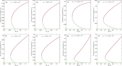
Figure 3. A plot of the basic reproduction number, ${\mathcal{R}}_m$, and the critical number ${\mathcal{R}}_m^c$ against bed-net coverage, b ((a) and (c)), and treatment rate u ((b) and (d)), for ${\mu }_m\in \{3.454\times {10}^{-4},4\times 3.454\times {10}^{-4}\}$. The saddle-node bifurcation value, ${\mathcal{R}}_m^{\ast }$, is at the intersection of the curves for ${\mathcal{R}}_m$ and ${\mathcal{R}}_m^c$. Solid blue line shows the basic reproduction number ${\mathcal{R}}_m$, the solid red line for ${\mathcal{R}}_m^c$ and the dashed horizontal green line denoted by ${\mathcal{R}}_m^1$ is a basic reproduction number of value unity.

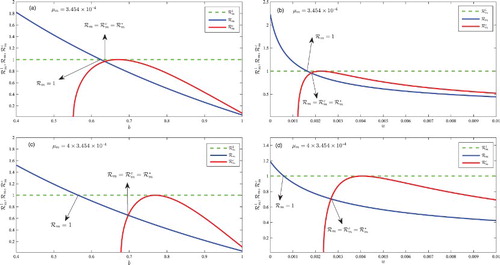
The saddle-node bifurcation value ${\mathcal{R}}_m^{\ast }$ has a crucial importance in terms of disease control. Figure 3 represents a plot of the basic reproduction number, ${\mathcal{R}}_m$, and the critical value, ${\mathcal{R}}_m^c$ against bed-net coverage, b, and treatment rate, u. In Figure 3(a), the saddle-node bifurcation value, ${\mathcal{R}}_m^{\ast }$, corresponds with a bed-net coverage of approximately b=0.635 and the basic reproduction number ${\mathcal{R}}_m$ is unity at approximately b=0.625. In this case, when bed-net coverage is between b=0.625 and b=0.635, a stable DFE coexists with two endemic equilibria. In Figure 3(c), the malaria-induced death rate is increased from ${\mu }_m=3.454\times {10}^{-4}$ to ${\mu }_m=4\times 3.454\times {10}^{-4}$; as a result, a stable DFE coexists with two endemic equilibria when the bed-net coverage is between b=0.565 and b=0.698. Hence, our result indicates that approximately $63.5\mathrm{\%}$ bed-net coverage might be required to control malaria when malaria-induced death rate is low (or ${\mu }_m=3.454\times {10}^{-4}$), and about $69.8\mathrm{\%}$ bed-net coverage when malaria-induced death rate is high (or ${\mu }_m=4\times 3.454\times {10}^{-4}$). Figure 3(b) and 3(d) shows that the DFE coexists with two endemic equilibrium when malaria treatment rate is between u=0.00162 and u=0.00182 and ${\mu }_m=3.454\times {10}^{-4}$; and between u=0.0006 and u=0.0027 when ${\mu }_m=4\times 3.454\times {10}^{-4}$. The implication of the results in Figures 2 and 3 is that in an environment with high malaria-induced death rate, more bed-net and treatment control efforts are required to contain the disease.

We prove the occurrence of backward bifurcation using the centre manifold theory as in [4, 5, 13]. We assume that $p_{hv}=p_{hv}^{\ast }$ is chosen as a bifurcation parameter, and consider the case ${\mathcal{R}}_h<{\mathcal{R}}_m=1$, then solving for $p_{hv}$ from ${\mathcal{R}}_m=1$, we have: $p_{hv}^{\ast }=\left[\right({\mu }_v\left(b\right){)}^2{K}_0{\mathrm{\Lambda }}_h\left]/\right[\left(\beta \right(b\left){)}^2{p}_{vh}{\mathrm{\Lambda }}_v\mu \right]$. Let ${\mathcal{J}}_{{p_{hv}}^{\ast }}^{hm}$ denote the Jacobian matrix of the system (1(1) $\begin{array}{rl}\dot{S}& ={\mathrm{\Lambda }}_h+\sigma u{I}_m+\rho R_m-({\lambda }_h+{\omega }_h+{\alpha }_1{\omega }_{hm}+\mu )S\\ {\dot{I}}_m& ={\lambda }_{h}S-({\omega }_h+{\alpha }_2{\omega }_{hm}+\gamma +u+{\mu }_m+\mu )I_m\\ {\dot{R}}_m& =(\gamma +(1-\sigma \left)u\right)I_m-({\omega }_h+{\alpha }_1{\omega }_{hm}+\rho +\mu )R_m\\ {\dot{I}}_{hm}& =({\omega }_h+{\alpha }_2{\omega }_{hm})I_m+{\alpha }_3{\lambda }_h{I}_h-({\kappa }_1\gamma +u+{\mu }_{hm}+\mu )I_{hm}\\ {\dot{R}}_{hm}& =\left(\right(1-\sigma )u+{\kappa }_1\gamma )I_{hm}+({\omega }_h+{\alpha }_1{\omega }_{hm})R_m-({\kappa }_2\rho +{\mu }_h+\mu )R_{hm}\\ {\dot{I}}_h& =\sigma u{I}_{hm}+{\kappa }_2\rho R_{hm}+({\omega }_h+{\alpha }_1{\omega }_{hm})S-({\alpha }_3{\lambda }_h+{\mu }_h+\mu )I_h\\ {\dot{S}}_v& ={\mathrm{\Lambda }}_v-({\lambda }_v^m+{\alpha }_4{\lambda }_v^{hm}+{\mu }_v(b\left)\right)S_v\\ {\dot{I}}_v& =({\lambda }_v^m+{\alpha }_4{\lambda }_v^{hm})S_v-{\mu }_v\left(b\right)I_v,\end{array}$(1) ) evaluated at $E_{df}$ with $p_{hv}=p_{hv}^{\ast }$, then ${\mathcal{J}}_{p_{hv}^{\ast }}^{hm}=\left(\begin{array}{cccccccc}-\mu & \sigma u& \rho & -{\alpha }_1{\beta }_h& -{\beta }_h& -{\beta }_h& 0& -p_{vh}\beta \left(b\right)\\ 0& -K_0& 0& 0& 0& 0& & p_{vh}\beta \left(b\right)\\ 0& K_1& -K_2& 0& 0& 0& 0& 0\\ 0& 0& 0& -K_3& 0& 0& 0& 0\\ 0& 0& 0& K_4& -K_5& 0& 0& 0\\ 0& 0& 0& {\beta }_h{\alpha }_1+\sigma u& {\kappa }_2\rho +{\beta }_h& {\beta }_h-K_6& 0& 0\\ 0& -\frac{{\mu }_v\left(b\right)K_0}{\beta \left(b\right)p_{vh}}& 0& -\frac{{\alpha }_4{\mu }_v\left(b\right)K_0}{\beta \left(b\right)p_{vh}}& 0& 0& -{\mu }_v\left(b\right)& 0\\ 0& \frac{{\mu }_v\left(b\right)K_0}{\beta \left(b\right)p_{vh}}& 0& \frac{{\alpha }_4{\mu }_v\left(b\right)K_0}{\beta \left(b\right)p_{vh}}& 0& 0& 0& -{\mu }_v\left(b\right)\end{array}\right).$

The eigenvalues of ${\mathcal{J}}_{{p_{hv}}^{\ast }}^{hm}$ are: $-\mu$, 0, $-{\mu }_v\left(b\right)$, $-K_5$, $-K_3$, $-K_2$, $-K_0-{\mu }_v\left(b\right)$ and ${\beta }_h-K_6$. From ${\mathcal{R}}_h<1$, ${\beta }_h-K_6<0$; it follows that the DFE, $E_{df}$, is non-hyperbolic. Thus, the centre manifold theory [4] can be used to investigate the occurrence of backward bifurcation. If the right and left eignvectors corresponding to the zero eigenvalue are $\tilde{w}$ and $\tilde{v}$, respectively, such that $\tilde{w}.\tilde{v}=1$, then $\begin{array}{rl}\tilde{w}& ={\left(\frac{\beta \left(b\right)p_{vh}}{\mu }\left(\frac{1}{K_0}\left(\sigma u+\rho \frac{K_1}{K_2}\right)-1\right),\frac{\beta \left(b\right)p_{vh}}{K_0},\frac{\beta \left(b\right)p_{vh}{K}_1}{K_0{K}_2},0,0,0,-1,1\right)}^T\\ \tilde{v}& =\left(0,\frac{{\mu }_v\left(b\right)K_0}{\beta \left(b\right)p_{vh}(K_0+{\mu }_v(b\left)\right)},0,\frac{{\alpha }_4{\mu }_v\left(b\right)K_0^2}{\beta \left(b\right)p_{vh}{K}_3(K_0+{\mu }_v(b\left)\right)},0,0,0,\frac{K_0}{K_0+{\mu }_v\left(b\right)}\right).\end{array}$ After some algebraic manipulations, the constants $a_1$ and $b_1$ (or $a_0$ and $b_0$ as in Theorem A.1) are: (15) $\begin{array}{rl}{a}_1& =\frac{2{\mu }_v\left(b\right)\beta \left(b\right)\mu p_{vh}}{{\mathrm{\Lambda }}_h(K_0+{\mu }_v(b\left)\right)}(B_1-B_2),\text{and}\\ b_1& =\frac{\beta \left(b\right)\mu {\mathrm{\Lambda }}_v}{{\mathrm{\Lambda }}_h{\mu }_v\left(b\right)}{\tilde{w}}_2{\tilde{v}}_8,\end{array}$(15) where $B_1=\left(K_0/\mu \right)[1-(1/K_0\left)\right(\sigma u+\rho \left(K_1/K_2\right)\left)\right]$, $B_2=[1+2(1+K_1/K_2)+{\mu }_v(b\left)K_0{\mathrm{\Lambda }}_h/\beta \left(b\right)\mu p_{vh}{\mathrm{\Lambda }}_v\right]$, ${\tilde{w}}_2=\beta \left(b\right)p_{vh}/K_0$ and ${\tilde{v}}_8=K_0/(K_0+{\mu }_v(b\left)\right)$.

Since $b_1>0$, the occurrence of backward bifurcation depends on the sign of $a_1$ (or the sign of $(B1-B2)$), and by Theorem A.1 the following result is established.

Theorem 3.3.

If (16) ${\mathrm{\Delta }}_m=\frac{K_0}{\mu }\left[1-\frac{1}{K_0}\left(\sigma u+\rho \frac{K_1}{K_2}\right)\right]-\left[1+2\left(1+\frac{K_1}{K_2}\right)+\frac{{\mu }_v\left(b\right)K_0{\mathrm{\Lambda }}_h}{\beta \left(b\right)\mu p_{vh}{\mathrm{\Lambda }}_v}\right],$(16) then the system (1(1) $\begin{array}{rl}\dot{S}& ={\mathrm{\Lambda }}_h+\sigma u{I}_m+\rho R_m-({\lambda }_h+{\omega }_h+{\alpha }_1{\omega }_{hm}+\mu )S\\ {\dot{I}}_m& ={\lambda }_{h}S-({\omega }_h+{\alpha }_2{\omega }_{hm}+\gamma +u+{\mu }_m+\mu )I_m\\ {\dot{R}}_m& =(\gamma +(1-\sigma \left)u\right)I_m-({\omega }_h+{\alpha }_1{\omega }_{hm}+\rho +\mu )R_m\\ {\dot{I}}_{hm}& =({\omega }_h+{\alpha }_2{\omega }_{hm})I_m+{\alpha }_3{\lambda }_h{I}_h-({\kappa }_1\gamma +u+{\mu }_{hm}+\mu )I_{hm}\\ {\dot{R}}_{hm}& =\left(\right(1-\sigma )u+{\kappa }_1\gamma )I_{hm}+({\omega }_h+{\alpha }_1{\omega }_{hm})R_m-({\kappa }_2\rho +{\mu }_h+\mu )R_{hm}\\ {\dot{I}}_h& =\sigma u{I}_{hm}+{\kappa }_2\rho R_{hm}+({\omega }_h+{\alpha }_1{\omega }_{hm})S-({\alpha }_3{\lambda }_h+{\mu }_h+\mu )I_h\\ {\dot{S}}_v& ={\mathrm{\Lambda }}_v-({\lambda }_v^m+{\alpha }_4{\lambda }_v^{hm}+{\mu }_v(b\left)\right)S_v\\ {\dot{I}}_v& =({\lambda }_v^m+{\alpha }_4{\lambda }_v^{hm})S_v-{\mu }_v\left(b\right)I_v,\end{array}$(1) ) undergoes backward bifurcation at ${\mathcal{R}}_0=1$ whenever ${\mathrm{\Delta }}_m>0,$ and forward bifurcation at ${\mathcal{R}}_0=1$ whenever ${\mathrm{\Delta }}_m<0$.

The possibility of backward bifurcation is explored numerically in Figure 4 for a high disease-induced mortality rate for both malaria and HIV. We set ${\mu }_m=2\times 3.454\times {10}^{-4}$, ${\mu }_h=2\times 2.3\times {10}^{-4}$. In Figure 4(a)–(c), we set u=0.0001 and for all values of b in $\{0.77,0.85,0.88,0.93\}$, the basic reproduction number ${\mathcal{R}}_0$ is below unity (i.e. ${\mathcal{R}}_m<1$ and ${\mathcal{R}}_h<1$). When b=0.77, at equilibrium, both malaria and HIV are endemic (dashed green curve). This suggests a backward bifurcation phenomena and the phenomena is confirmed since ${\mathrm{\Delta }}_m=10.39>0$. Also, backward bifurcation is exhibited when bed-net coverage is increased to b=0.85 (dashed black curve) and b=0.88 (dashed red curve); also, ${\mathrm{\Delta }}_m=10.13>0$ when b=0.85, and ${\mathrm{\Delta }}_m=9.9497>0$ when b=0.88, backward bifurcation is confirmed. When bed-net coverage b is increased from 77% to 85%, the proportion of malaria-only infected ($I_m$) individuals at the endemic equilibrium decreases, but the proportion of HIV-infected individuals increase. This is attributed to an increase in the pool of malaria susceptibility. Also, the pool of malaria-infected individuals decreases with an increase in bet-net coverage, which results in an increase in the proportion of HIV-only infected ($I_h$) individuals. Since by assumption malaria transmission rate in HIV infected individuals is higher than in HIV-free individuals, the number of malaria-HIV co-infected individuals increases as bed-net coverage increases in this case. The phenomena is the same as bed-net coverage increases from 85% to 88%. If bed-net coverage increases further to 93%, both malaria and HIV are eradicated at equilibrium (Solid blue curves). In this case, bed-net coverage at 93% reduces contact between mosquitoes and humans significantly, and both diseases are eradicated. Even though HIV and malaria have different transmission mechanisms, high bed-net coverage for malaria control at 93% will minimize significantly malaria-HIV co-infection and in the absence of co-infection, HIV will be eradicated, since ${\mathcal{R}}_h<1$. However, when bed-net coverage is not high enough to eliminate malaria, HIV will be endemic due to the amplification effect caused by co-infection. This result is consistent with the results reported in [9, 10]. These results suggest that bed-net control for malaria with high coverage can help to control both malaria and HIV wherever the two infections coexist.

Figure 4. Numerical simulations illustrating that system (1(1) $\begin{array}{rl}\dot{S}& ={\mathrm{\Lambda }}_h+\sigma u{I}_m+\rho R_m-({\lambda }_h+{\omega }_h+{\alpha }_1{\omega }_{hm}+\mu )S\\ {\dot{I}}_m& ={\lambda }_{h}S-({\omega }_h+{\alpha }_2{\omega }_{hm}+\gamma +u+{\mu }_m+\mu )I_m\\ {\dot{R}}_m& =(\gamma +(1-\sigma \left)u\right)I_m-({\omega }_h+{\alpha }_1{\omega }_{hm}+\rho +\mu )R_m\\ {\dot{I}}_{hm}& =({\omega }_h+{\alpha }_2{\omega }_{hm})I_m+{\alpha }_3{\lambda }_h{I}_h-({\kappa }_1\gamma +u+{\mu }_{hm}+\mu )I_{hm}\\ {\dot{R}}_{hm}& =\left(\right(1-\sigma )u+{\kappa }_1\gamma )I_{hm}+({\omega }_h+{\alpha }_1{\omega }_{hm})R_m-({\kappa }_2\rho +{\mu }_h+\mu )R_{hm}\\ {\dot{I}}_h& =\sigma u{I}_{hm}+{\kappa }_2\rho R_{hm}+({\omega }_h+{\alpha }_1{\omega }_{hm})S-({\alpha }_3{\lambda }_h+{\mu }_h+\mu )I_h\\ {\dot{S}}_v& ={\mathrm{\Lambda }}_v-({\lambda }_v^m+{\alpha }_4{\lambda }_v^{hm}+{\mu }_v(b\left)\right)S_v\\ {\dot{I}}_v& =({\lambda }_v^m+{\alpha }_4{\lambda }_v^{hm})S_v-{\mu }_v\left(b\right)I_v,\end{array}$(1) ). The vertical axis represents proportion of population: in (a) and (d) malaria-infected human population; in (b) and (e) HIV human population; and in (c) and (f) malaria-infected mosquito. We set ${\mu }_m=2\times 3.454\times {10}^{-4}$ and ${\mu }_h=2\times 2.3\times {10}^{-4}$ (i.e. a higher malaria and HIV-induced death rates). (i) In (a)–(c) bed-net coverage values are $b\in \{0.77,0.85,0.88,0.93\}$. Backward bifurcation occurs for b=0.77,0.85 and b=0.88, however, long-term dynamics of the model system (1(1) $\begin{array}{rl}\dot{S}& ={\mathrm{\Lambda }}_h+\sigma u{I}_m+\rho R_m-({\lambda }_h+{\omega }_h+{\alpha }_1{\omega }_{hm}+\mu )S\\ {\dot{I}}_m& ={\lambda }_{h}S-({\omega }_h+{\alpha }_2{\omega }_{hm}+\gamma +u+{\mu }_m+\mu )I_m\\ {\dot{R}}_m& =(\gamma +(1-\sigma \left)u\right)I_m-({\omega }_h+{\alpha }_1{\omega }_{hm}+\rho +\mu )R_m\\ {\dot{I}}_{hm}& =({\omega }_h+{\alpha }_2{\omega }_{hm})I_m+{\alpha }_3{\lambda }_h{I}_h-({\kappa }_1\gamma +u+{\mu }_{hm}+\mu )I_{hm}\\ {\dot{R}}_{hm}& =\left(\right(1-\sigma )u+{\kappa }_1\gamma )I_{hm}+({\omega }_h+{\alpha }_1{\omega }_{hm})R_m-({\kappa }_2\rho +{\mu }_h+\mu )R_{hm}\\ {\dot{I}}_h& =\sigma u{I}_{hm}+{\kappa }_2\rho R_{hm}+({\omega }_h+{\alpha }_1{\omega }_{hm})S-({\alpha }_3{\lambda }_h+{\mu }_h+\mu )I_h\\ {\dot{S}}_v& ={\mathrm{\Lambda }}_v-({\lambda }_v^m+{\alpha }_4{\lambda }_v^{hm}+{\mu }_v(b\left)\right)S_v\\ {\dot{I}}_v& =({\lambda }_v^m+{\alpha }_4{\lambda }_v^{hm})S_v-{\mu }_v\left(b\right)I_v,\end{array}$(1) ) shows a stable DFE when bed-net coverage is increased to b=0.93; (ii) in (d)–(f) malaria treatment rate values are $u\in \{0.0001,0.0002,0.0003,0.003\}$. Backward bifurcation occurs for u=0.0001,0.0005 and u=0.001, however, long-term dynamics of system (1(1) $\begin{array}{rl}\dot{S}& ={\mathrm{\Lambda }}_h+\sigma u{I}_m+\rho R_m-({\lambda }_h+{\omega }_h+{\alpha }_1{\omega }_{hm}+\mu )S\\ {\dot{I}}_m& ={\lambda }_{h}S-({\omega }_h+{\alpha }_2{\omega }_{hm}+\gamma +u+{\mu }_m+\mu )I_m\\ {\dot{R}}_m& =(\gamma +(1-\sigma \left)u\right)I_m-({\omega }_h+{\alpha }_1{\omega }_{hm}+\rho +\mu )R_m\\ {\dot{I}}_{hm}& =({\omega }_h+{\alpha }_2{\omega }_{hm})I_m+{\alpha }_3{\lambda }_h{I}_h-({\kappa }_1\gamma +u+{\mu }_{hm}+\mu )I_{hm}\\ {\dot{R}}_{hm}& =\left(\right(1-\sigma )u+{\kappa }_1\gamma )I_{hm}+({\omega }_h+{\alpha }_1{\omega }_{hm})R_m-({\kappa }_2\rho +{\mu }_h+\mu )R_{hm}\\ {\dot{I}}_h& =\sigma u{I}_{hm}+{\kappa }_2\rho R_{hm}+({\omega }_h+{\alpha }_1{\omega }_{hm})S-({\alpha }_3{\lambda }_h+{\mu }_h+\mu )I_h\\ {\dot{S}}_v& ={\mathrm{\Lambda }}_v-({\lambda }_v^m+{\alpha }_4{\lambda }_v^{hm}+{\mu }_v(b\left)\right)S_v\\ {\dot{I}}_v& =({\lambda }_v^m+{\alpha }_4{\lambda }_v^{hm})S_v-{\mu }_v\left(b\right)I_v,\end{array}$(1) ) show a stable DFE when malaria treatment rate is increased to u=0.003.

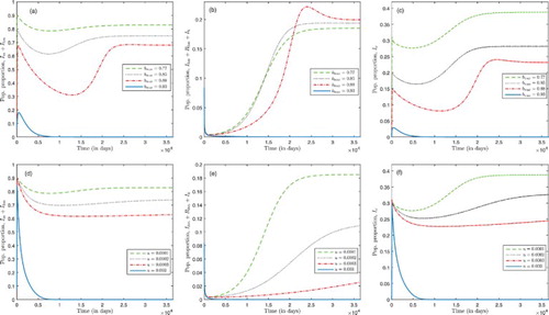
In Figure 4(d)–(f), we set b=0.77 and for all values $u\in \{0.0001,0.0002,0.0003,0.003\}$ the basic reproduction number ${\mathcal{R}}_0$ is below unity. For u=0.0001, at equilibrium, both malaria and HIV are endemic (dashed green curve) which suggests the occurrence of backward bifurcation phenomena and is confirmed since ${\mathrm{\Delta }}_m=10.39>0$. This also occurs when malaria treatment rate is increased to u=0.0002 (dashed black curve) and u=0.0003 (dashed red curve) at which ${\mathrm{\Delta }}_m=10.31>0$ and ${\mathrm{\Delta }}_m=10.23>0$, respectively. The proportion of malaria and HIV infected as well as co-infected humans decreases as the treatment rate u increases from 0.0001 to 0.0002, and also the proportion of malaria-only infected individuals decreases. The same phenomena is observed when the malaria treatment rate is increased from 0.0002 to 0.0003. However, for a higher malaria treatment rate, u=0.003, both malaria and HIV are eradicated at equilibrium (solid blue curve). This result suggests that malaria treatment at a higher rate can reduce disease burden, for both malaria and HIV, where there is malaria-HIV co-infection. Furthermore, for these parameter regimes when malaria treatment rate is low, there will be an increase in the proportion of malaria and HIV infected as well as co-infected humans. For the set of parameter values used, our results in Figure 4 suggest that the parameters representing bed-net coverage and malaria treatment rate are important parameters in the control of malaria and HIV infections in an environment where both diseases coexist.

From Equation (16(16) ${\mathrm{\Delta }}_m=\frac{K_0}{\mu }\left[1-\frac{1}{K_0}\left(\sigma u+\rho \frac{K_1}{K_2}\right)\right]-\left[1+2\left(1+\frac{K_1}{K_2}\right)+\frac{{\mu }_v\left(b\right)K_0{\mathrm{\Lambda }}_h}{\beta \left(b\right)\mu p_{vh}{\mathrm{\Lambda }}_v}\right],$(16) ), we observe that the occurrence of backward bifurcation is influenced by the malaria disease mortality rate, ${\mu }_m$, the bed-net coverage parameter, b, and malaria treatment rate, u. To identify the important parameters in the disease control we carry out a sensitivity analysis. Following the approach in [8], we compute the sensitivity index for the basic reproduction number, ${\mathcal{R}}_m$, that depends differentially on a parameter, p, as: $\left(\mathrm{\partial }{\mathcal{R}}_m/\mathrm{\partial }p\right)\times \left(p/{\mathcal{R}}_m\right)$. The sensitivity index measures the ratio of relative changes on the basic reproduction number, ${\mathcal{R}}_m$, with respect to changes in the parameter p; it is most sensitive to the parameter with the largest sensitivity index value (in magnitude) and least sensitive to the parameter with the smallest sensitivity index value (in magnitude). The sensitivity indices of the basic reproduction number, ${\mathcal{R}}_m$, with respect to the model parameters are listed in Table 2. The parameter values are set at: b=0.65, u=0.002 and other parameters are the same as in Table 1.

The basic reproduction number ${\mathcal{R}}_m$ is most sensitive to the bed-net coverage, b, maximum mosquito biting rate, ${\beta }_{\max }$, mosquito death rate ${\mu }_{v0}$, death rate of humans, μ, and malaria treatment rate u. Qualitatively, the basic reproduction number decreases by 21.49% for an increase in bed-net coverage by 10%, ${\mathcal{R}}_m$ is decreased by 6.06% when mosquito death rate is increased by 10%, and a 10% increase in malaria treatment rate decreases the basic reproduction number by 4.15%. The implication of these results is that insecticide-treated nets, vector control and malaria treatment are important in the control of malaria.

In Section 4, we formulate and investigate optimal malaria treatment and insecticide-treated bed-net strategies, and the possibility of controlling the malaria-HIV co-infection using malaria treatment and insecticide-treated nets at a minimum cost, and within a short control period of time.

4. Optimal control formulation and analysis

4.1. Optimal control formulation

In order to determine the optimal strategy for treatment of malaria-infected individuals, and bed-net coverage, we redefine the treatment rate, u, in system (1(1) $\begin{array}{rl}\dot{S}& ={\mathrm{\Lambda }}_h+\sigma u{I}_m+\rho R_m-({\lambda }_h+{\omega }_h+{\alpha }_1{\omega }_{hm}+\mu )S\\ {\dot{I}}_m& ={\lambda }_{h}S-({\omega }_h+{\alpha }_2{\omega }_{hm}+\gamma +u+{\mu }_m+\mu )I_m\\ {\dot{R}}_m& =(\gamma +(1-\sigma \left)u\right)I_m-({\omega }_h+{\alpha }_1{\omega }_{hm}+\rho +\mu )R_m\\ {\dot{I}}_{hm}& =({\omega }_h+{\alpha }_2{\omega }_{hm})I_m+{\alpha }_3{\lambda }_h{I}_h-({\kappa }_1\gamma +u+{\mu }_{hm}+\mu )I_{hm}\\ {\dot{R}}_{hm}& =\left(\right(1-\sigma )u+{\kappa }_1\gamma )I_{hm}+({\omega }_h+{\alpha }_1{\omega }_{hm})R_m-({\kappa }_2\rho +{\mu }_h+\mu )R_{hm}\\ {\dot{I}}_h& =\sigma u{I}_{hm}+{\kappa }_2\rho R_{hm}+({\omega }_h+{\alpha }_1{\omega }_{hm})S-({\alpha }_3{\lambda }_h+{\mu }_h+\mu )I_h\\ {\dot{S}}_v& ={\mathrm{\Lambda }}_v-({\lambda }_v^m+{\alpha }_4{\lambda }_v^{hm}+{\mu }_v(b\left)\right)S_v\\ {\dot{I}}_v& =({\lambda }_v^m+{\alpha }_4{\lambda }_v^{hm})S_v-{\mu }_v\left(b\right)I_v,\end{array}$(1) ) as a function of time, $u\left(t\right)$. The force of infections ${\lambda }_h$, ${\lambda }_v^m$ and ${\lambda }_v^{hm}$ for malaria transmission, and the mortality rate of mosquitoes, ${\mu }_v\left(b\right)$ in system (1(1) $\begin{array}{rl}\dot{S}& ={\mathrm{\Lambda }}_h+\sigma u{I}_m+\rho R_m-({\lambda }_h+{\omega }_h+{\alpha }_1{\omega }_{hm}+\mu )S\\ {\dot{I}}_m& ={\lambda }_{h}S-({\omega }_h+{\alpha }_2{\omega }_{hm}+\gamma +u+{\mu }_m+\mu )I_m\\ {\dot{R}}_m& =(\gamma +(1-\sigma \left)u\right)I_m-({\omega }_h+{\alpha }_1{\omega }_{hm}+\rho +\mu )R_m\\ {\dot{I}}_{hm}& =({\omega }_h+{\alpha }_2{\omega }_{hm})I_m+{\alpha }_3{\lambda }_h{I}_h-({\kappa }_1\gamma +u+{\mu }_{hm}+\mu )I_{hm}\\ {\dot{R}}_{hm}& =\left(\right(1-\sigma )u+{\kappa }_1\gamma )I_{hm}+({\omega }_h+{\alpha }_1{\omega }_{hm})R_m-({\kappa }_2\rho +{\mu }_h+\mu )R_{hm}\\ {\dot{I}}_h& =\sigma u{I}_{hm}+{\kappa }_2\rho R_{hm}+({\omega }_h+{\alpha }_1{\omega }_{hm})S-({\alpha }_3{\lambda }_h+{\mu }_h+\mu )I_h\\ {\dot{S}}_v& ={\mathrm{\Lambda }}_v-({\lambda }_v^m+{\alpha }_4{\lambda }_v^{hm}+{\mu }_v(b\left)\right)S_v\\ {\dot{I}}_v& =({\lambda }_v^m+{\alpha }_4{\lambda }_v^{hm})S_v-{\mu }_v\left(b\right)I_v,\end{array}$(1) ) are modelled in the presence of constant insecticide-treated bed-net coverage. Thus, we incorporate control by redefining the constant bed-net coverage, b, as a function of time, $b\left(t\right)$, so that the biting and mortality rates of mosquitoes are $\beta \left(b\right(t\left)\right)={\beta }_{max}-({\beta }_{max}-{\beta }_{min})b\left(t\right)\text{and}{\mu }_v\left(b\right(t\left)\right)={\mu }_{v0}+{\mu }_{v1}b\left(t\right),$ respectively. The forces of infection for malaria transmission become: (17) ${\tilde{\lambda }}_h\left(t\right)=\frac{p_{vh}\beta \left(b\right(t\left)\right)I_v\left(t\right)}{N\left(t\right)},{\tilde{\lambda }}_v^m\left(t\right)=\frac{p_{hv}\beta \left(b\right(t\left)\right)I_m\left(t\right)}{N\left(t\right)},{\tilde{\lambda }}_v^{hm}\left(t\right)=\frac{p_{hv}\beta \left(b\right(t\left)\right)I_{hm}\left(t\right)}{N\left(t\right)}.$(17) The control $u\left(t\right)=0$ corresponds to no treatment, and $u\left(t\right)=1$ indicates that treatment is at its maximum level. On the other hand, when $b\left(t\right)=0$, there is no reduction in transmission due to the absence of insecticide-treated bed-net coverage, and mosquitoes die naturally. When $b\left(t\right)=1$, there is perfect coverage for humans resulting from treated bed-net usage, and mosquitoes questing for a blood meal experience an insecticide-induced death. In our analysis and numerical simulations, we shall assume that $b\left(t\right)\in [0,1)$ for all t>0. Thus, the malaria-HIV co-infection model incorporating insecticide-treated bed-net coverage in the presence of malaria treatment of humans infected with malaria and co-infected with malaria and HIV as control functions is: (18) $\begin{array}{rl}\dot{S}& ={\mathrm{\Lambda }}_h+\sigma u\left(t\right)I_m+\rho R_m-({\tilde{\lambda }}_h+{\omega }_h+{\alpha }_1{\omega }_{hm}+\mu )S,\\ {\dot{I}}_m& ={\tilde{\lambda }}_{h}S-({\omega }_h+{\alpha }_2{\omega }_{hm}+\gamma +u(t)+{\mu }_m+\mu )I_m,\\ {\dot{R}}_m& =(\gamma +(1-\sigma \left)u\right(t\left)\right)I_m-({\omega }_h+{\alpha }_1{\omega }_{hm}+\rho +\mu )R_m,\\ {\dot{I}}_{hm}& =({\omega }_h+{\alpha }_2{\omega }_{hm})I_m+{\alpha }_3{\tilde{\lambda }}_h{I}_h-({\kappa }_1\gamma +u(t)+{\mu }_{hm}+\mu )I_{hm},\\ {\dot{R}}_{hm}& =(1-\sigma )u\left(t\right)I_{hm}+{\kappa }_1\gamma I_{hm}+({\omega }_h+{\alpha }_1{\omega }_{hm})R_m-({\kappa }_2\rho +{\mu }_h+\mu )R_{hm,}\\ {\dot{I}}_h& =\sigma u\left(t\right)I_{hm}+{\kappa }_2\rho R_{hm}+({\omega }_h+{\alpha }_1{\omega }_{hm})S-({\alpha }_3{\tilde{\lambda }}_h+{\mu }_h+\mu )I_h,\\ {\dot{S}}_v& ={\mathrm{\Lambda }}_v-({\tilde{\lambda }}_v^m+{\alpha }_4{\tilde{\lambda }}_v^{hm}+{\mu }_v(b\left(t\right)\left)\right)S_v,\\ {\dot{I}}_v& =({\tilde{\lambda }}_v^m+{\alpha }_4{\tilde{\lambda }}_v^{hm})S_v-{\mu }_v\left(b\right(t\left)\right)I_v,\end{array}$(18) with initial conditions (19) $\begin{array}{rl}S\left(0\right)& =S^0,I_m\left(0\right)=I_m^0,R_m\left(0\right)=R_m^0,I_{hm}\left(0\right)=I_{hm}^0,\\ R_{hm}\left(0\right)& =R_{hm}^0,I_h\left(0\right)=I_h^0,S_v\left(0\right)=S_v^0,I_v\left(0\right)=I_v^0.\end{array}$(19) We formulate our optimal control problem, which seeks to minimize the number humans infected with malaria, co-infected with malaria and HIV, the number of infectious mosquitoes, and the cost of treatment and bed-net coverage. To do this, we construct the following objective functional (20) $\begin{array}{rl}J(b,u)& ={\int }_0^T\left(A_1{I}_m\right(t)+A_2{I}_{hm}(t)+A_3{I}_v(t\left)\right)\mathrm{d}t\\ & +{\int }_0^T(+B_{1}u(t\left)I_m\right(t)+B_{2}u(t\left)I_{hm}\right(t)+B_{3}b(t\left)N\right(t\left)\right)\mathrm{d}t\\ & +{\int }_0^T\left(C_1{u}^2\right(t)+C_2{b}^2(t\left)\right)\mathrm{d}t,\end{array}$(20) where $[0,T]$ is the entire time horizon over which treatment and insecticide-treated nets are applied, and the constants $A_i,B_i,C_j$ for $i=1,2,\dots ,3$, j=1,2, are positive constants that balance the relative importance of terms in the objective functional J. The term ${\int }_0^T\left(A_1{I}_m\right(t)+A_2{I}_{hm}(t)+A_3{I}_v(t\left)\right)\mathrm{d}t$ gives the number of humans infected with malaria and co-infected with malaria and HIV, and the total number of infected mosquitoes over the time period T being modelled. The term $u\left(t\right)\left(I_m\right(t)+I_{hm}(t\left)\right)$ depicts the total number of humans receiving the malaria treatment, so that ${\int }_0^T\left(B_{1}u\right(t\left)I_m\right(t)+B_{2}u(t\left)I_{hm}\right(t)+C_1{u}^2(t\left)\right)\mathrm{d}t$ gives the total cost of malaria treatment for malaria-infected and malaria-HIV co-infected individuals in the population. The constants $B_1$ and $B_2$ are the respective costs of treatment per individual infected with malaria and co-infected with malaria and HIV. Finally, ${\int }_0^T\left(B_{3}b\right(t\left)N\right(t)+C_2{b}^2(t)\mathrm{d}t$ represents the cost of introducing insecticide-treated nets in the population over the time period T. Our optimal control problem is: Find $(b^{\ast },u^{\ast })\in \mathcal{U}$ such that $J(b^{\ast },u^{\ast })=\underset{(b,u)\in \mathcal{U}}{inf}J(b,u),$ where the set of all admissible controls, $\mathcal{U}$, is defined as $\mathcal{U}=\left\{\right(b,u)\in (L^{\mathrm{\infty }}(0,T){)}^2|0\le b\left(t\right)\le b_{max},0\le u\left(t\right)\le u_{max};b,u\mathrm{Lebesguemeasurable}\}.$

4.2. Positivity and boundedness of state solutions

With our formulation of the optimal control problem, we prove the existence of a non-negative, bounded solution.

Theorem 4.1.

Given positive initial conditions (19(19) $\begin{array}{rl}S\left(0\right)& =S^0,I_m\left(0\right)=I_m^0,R_m\left(0\right)=R_m^0,I_{hm}\left(0\right)=I_{hm}^0,\\ R_{hm}\left(0\right)& =R_{hm}^0,I_h\left(0\right)=I_h^0,S_v\left(0\right)=S_v^0,I_v\left(0\right)=I_v^0.\end{array}$(19) ), there exists a positive, bounded solution $(S,I_m,R_m,I_{hm},R_{hm},I_h,S_v,I_v)$ to the initial value problem (1(1) $\begin{array}{rl}\dot{S}& ={\mathrm{\Lambda }}_h+\sigma u{I}_m+\rho R_m-({\lambda }_h+{\omega }_h+{\alpha }_1{\omega }_{hm}+\mu )S\\ {\dot{I}}_m& ={\lambda }_{h}S-({\omega }_h+{\alpha }_2{\omega }_{hm}+\gamma +u+{\mu }_m+\mu )I_m\\ {\dot{R}}_m& =(\gamma +(1-\sigma \left)u\right)I_m-({\omega }_h+{\alpha }_1{\omega }_{hm}+\rho +\mu )R_m\\ {\dot{I}}_{hm}& =({\omega }_h+{\alpha }_2{\omega }_{hm})I_m+{\alpha }_3{\lambda }_h{I}_h-({\kappa }_1\gamma +u+{\mu }_{hm}+\mu )I_{hm}\\ {\dot{R}}_{hm}& =\left(\right(1-\sigma )u+{\kappa }_1\gamma )I_{hm}+({\omega }_h+{\alpha }_1{\omega }_{hm})R_m-({\kappa }_2\rho +{\mu }_h+\mu )R_{hm}\\ {\dot{I}}_h& =\sigma u{I}_{hm}+{\kappa }_2\rho R_{hm}+({\omega }_h+{\alpha }_1{\omega }_{hm})S-({\alpha }_3{\lambda }_h+{\mu }_h+\mu )I_h\\ {\dot{S}}_v& ={\mathrm{\Lambda }}_v-({\lambda }_v^m+{\alpha }_4{\lambda }_v^{hm}+{\mu }_v(b\left)\right)S_v\\ {\dot{I}}_v& =({\lambda }_v^m+{\alpha }_4{\lambda }_v^{hm})S_v-{\mu }_v\left(b\right)I_v,\end{array}$(1) ).

Proof.

Representation formulas for the solutions to the differential equations for $I_m$, $R_m$ and $S_v$ in system (1(1) $\begin{array}{rl}\dot{S}& ={\mathrm{\Lambda }}_h+\sigma u{I}_m+\rho R_m-({\lambda }_h+{\omega }_h+{\alpha }_1{\omega }_{hm}+\mu )S\\ {\dot{I}}_m& ={\lambda }_{h}S-({\omega }_h+{\alpha }_2{\omega }_{hm}+\gamma +u+{\mu }_m+\mu )I_m\\ {\dot{R}}_m& =(\gamma +(1-\sigma \left)u\right)I_m-({\omega }_h+{\alpha }_1{\omega }_{hm}+\rho +\mu )R_m\\ {\dot{I}}_{hm}& =({\omega }_h+{\alpha }_2{\omega }_{hm})I_m+{\alpha }_3{\lambda }_h{I}_h-({\kappa }_1\gamma +u+{\mu }_{hm}+\mu )I_{hm}\\ {\dot{R}}_{hm}& =\left(\right(1-\sigma )u+{\kappa }_1\gamma )I_{hm}+({\omega }_h+{\alpha }_1{\omega }_{hm})R_m-({\kappa }_2\rho +{\mu }_h+\mu )R_{hm}\\ {\dot{I}}_h& =\sigma u{I}_{hm}+{\kappa }_2\rho R_{hm}+({\omega }_h+{\alpha }_1{\omega }_{hm})S-({\alpha }_3{\lambda }_h+{\mu }_h+\mu )I_h\\ {\dot{S}}_v& ={\mathrm{\Lambda }}_v-({\lambda }_v^m+{\alpha }_4{\lambda }_v^{hm}+{\mu }_v(b\left)\right)S_v\\ {\dot{I}}_v& =({\lambda }_v^m+{\alpha }_4{\lambda }_v^{hm})S_v-{\mu }_v\left(b\right)I_v,\end{array}$(1) ) obtained by the method of integrating factors are: $\begin{array}{rl}{I}_m\left(t\right)& =I_m^0{\mathrm{e}}^{-{\int }_0^t(K_0+{\omega }_h(\xi )+{\alpha }_4{\omega }_{hm}(\xi \left)\right)\mathrm{d}\xi }+{\int }_0^t{\lambda }_h\left(s\right)S\left(s\right){\mathrm{e}}^{-{\int }_s^t(K_7+{\omega }_h(\xi )+{\alpha }_4{\omega }_{hm}(\xi \left)\right)\mathrm{d}\xi }\mathrm{d}s\\ R_m\left(t\right)& =R_m^0{\mathrm{e}}^{-{\int }_0^t\left({\omega }_h\right(r)+{\alpha }_1{\omega }_{hm}(r)+\rho +\mu )\mathrm{d}r}\\ & +(\gamma +(1-\sigma \left)u\right){\int }_0^t{I}_m\left(s\right){\mathrm{e}}^{-{\int }_s^t\left({\omega }_h\right(r)+{\alpha }_1{\omega }_{hm}(r)+\rho +\mu )\mathrm{d}r}\mathrm{d}s\\ S_v\left(t\right)& =S_v^0{\mathrm{e}}^{-{\int }_0^t\left({\lambda }_v^m\right(\xi )+{\alpha }_4{\lambda }_v^{hm}(\xi )+{\mu }_v(b\left)\right)\mathrm{d}\xi }+{\mathrm{\Lambda }}_v{\int }_0^t{\mathrm{e}}^{-{\int }_s^t\left({\lambda }_v^m\right(\xi )+{\alpha }_4{\lambda }_v^{hm}(\xi )+{\mu }_v(b\left)\right)\mathrm{d}\xi }\mathrm{d}s>0,\end{array}$ Assume that there exists $t_1>0$ such that $\begin{array}{rl}& S\left(t_1\right)>0,I_m\left(t_1\right)>0,R_m\left(t_1\right)>0,I_{hm}\left(t_1\right)>0,\\ & R_{hm}\left(t_1\right)>0,I_h\left(t_1\right)>0,I_v\left(t_1\right)>0,\end{array}$ on $[0,t_1)$, where $t_1$ is the first time any of the state functions hits zero. Now, if $R_m\left(t_1\right)=0$, then there exists an interval $({\tau }_1,{\tau }_2)\subset [0,t_1)$ with ${\tau }_1\ne {\tau }_2$ such that $I_m\left(s\right)<0$ for $s\in ({\tau }_1,{\tau }_2)$, which is absurd. Thus, $R_m\left(t\right)>0$ in $[0,t_1]$. Next, if $I_m\left(t_1\right)=0$, then there exists a sub-interval $({\tau }_1,{\tau }_2)\subset [0,t_1)$ with ${\tau }_1\ne {\tau }_2$ such that ${\lambda }_h\left(s\right)<0$ and $S\left(s\right)>0$ or ${\lambda }_h\left(s\right)>0$ and $S\left(s\right)<0$ for $s\in ({\tau }_1,{\tau }_2)$, which is absurd. Thus, $I_m\left(t\right)>0$ in $[0,t_1]$. Since $I_m\left(t\right)>0$ and $R_m\left(t\right)>0$ in $[0,t_1]$, it follows from the differential equation for S in system (1(1) $\begin{array}{rl}\dot{S}& ={\mathrm{\Lambda }}_h+\sigma u{I}_m+\rho R_m-({\lambda }_h+{\omega }_h+{\alpha }_1{\omega }_{hm}+\mu )S\\ {\dot{I}}_m& ={\lambda }_{h}S-({\omega }_h+{\alpha }_2{\omega }_{hm}+\gamma +u+{\mu }_m+\mu )I_m\\ {\dot{R}}_m& =(\gamma +(1-\sigma \left)u\right)I_m-({\omega }_h+{\alpha }_1{\omega }_{hm}+\rho +\mu )R_m\\ {\dot{I}}_{hm}& =({\omega }_h+{\alpha }_2{\omega }_{hm})I_m+{\alpha }_3{\lambda }_h{I}_h-({\kappa }_1\gamma +u+{\mu }_{hm}+\mu )I_{hm}\\ {\dot{R}}_{hm}& =\left(\right(1-\sigma )u+{\kappa }_1\gamma )I_{hm}+({\omega }_h+{\alpha }_1{\omega }_{hm})R_m-({\kappa }_2\rho +{\mu }_h+\mu )R_{hm}\\ {\dot{I}}_h& =\sigma u{I}_{hm}+{\kappa }_2\rho R_{hm}+({\omega }_h+{\alpha }_1{\omega }_{hm})S-({\alpha }_3{\lambda }_h+{\mu }_h+\mu )I_h\\ {\dot{S}}_v& ={\mathrm{\Lambda }}_v-({\lambda }_v^m+{\alpha }_4{\lambda }_v^{hm}+{\mu }_v(b\left)\right)S_v\\ {\dot{I}}_v& =({\lambda }_v^m+{\alpha }_4{\lambda }_v^{hm})S_v-{\mu }_v\left(b\right)I_v,\end{array}$(1) ) that $S\left(t\right)>0$ in $[0,t_1]$. By a similar argument, it follows that $I_{hm}\left(t\right)>0$, $R_{hm}\left(t\right)>0$, $I_h\left(t\right)>0$ and $I_v\left(t\right)>0$ in $[0,t_1]$. Hence the state functions are positive for t>0.

To prove boundedness of state functions, we consider differential equations for the total mosquito and human populations in Equation (2(2) ${\dot{N}}_h={\mathrm{\Lambda }}_h-{\mu }_h{N}_h-{\mu }_m{I}_m-{\mu }_{hm}{I}_{hm}-{\mu }_h(R_{hm}+I_h);{\dot{N}}_v={\mathrm{\Lambda }}_v-{\mu }_v\left(b\right)N_v.$(2) ). The following function satisfies the differential equation for $N_v$ is Equation (2(2) ${\dot{N}}_h={\mathrm{\Lambda }}_h-{\mu }_h{N}_h-{\mu }_m{I}_m-{\mu }_{hm}{I}_{hm}-{\mu }_h(R_{hm}+I_h);{\dot{N}}_v={\mathrm{\Lambda }}_v-{\mu }_v\left(b\right)N_v.$(2) ): $N_v\left(t\right)=N_v\left(0\right){\mathrm{e}}^{-{\mu }_v\left(b\right)t}+\frac{{\mathrm{\Lambda }}_v}{{\mu }_v\left(b\right)}(1-{\mathrm{e}}^{-{\mu }_v\left(b\right)t}).$ Therefore, $0<min\left\{N_v\left(0\right),\frac{{\mathrm{\Lambda }}_v}{{\mu }_v\left(b\right)}\right\}\le N_v\left(t\right)\le max\left\{N_v\left(0\right),\frac{{\mathrm{\Lambda }}_v}{{\mu }_v\left(b\right)}\right\},$ by convexity. Similarly, from the differential equation for the total human population given in Equation (2(2) ${\dot{N}}_h={\mathrm{\Lambda }}_h-{\mu }_h{N}_h-{\mu }_m{I}_m-{\mu }_{hm}{I}_{hm}-{\mu }_h(R_{hm}+I_h);{\dot{N}}_v={\mathrm{\Lambda }}_v-{\mu }_v\left(b\right)N_v.$(2) ), we obtain: $\dot{N}={\mathrm{\Lambda }}_h-\mu N-({\mu }_m{I}_m+{\mu }_{hm}{I}_{hm}+{\mu }_h{R}_{hm}+{\mu }_h{I}_h)\le {\mathrm{\Lambda }}_h-\mu N.$ Then, the standard comparison theorem of differential equations ([20], p. 31; [21], Theorem B.1; Appendix B) can be used to show that $N\left(t\right)\le N\left(0\right){\mathrm{e}}^{-\mu t}+\frac{{\mathrm{\Lambda }}_h}{\mu }(1-{\mathrm{e}}^{-\mu t}),$ which implies that $N\left(t\right)\le max\left\{N\right(0),{\mathrm{\Lambda }}_h/\mu \}$. Also, the total human population satisfies ${\mathrm{\Lambda }}_h-({\mu }_h+\tilde{\mu })N\le \frac{\mathrm{d}N}{\mathrm{d}t}\le {\mathrm{\Lambda }}_h-{\mu }_{h}N,$ Assuming that $\tilde{\mu }=max\{{\mu }_m,{\mu }_h,{\mu }_{hm}\}$, the solution of the total human population in Equation (2(2) ${\dot{N}}_h={\mathrm{\Lambda }}_h-{\mu }_h{N}_h-{\mu }_m{I}_m-{\mu }_{hm}{I}_{hm}-{\mu }_h(R_{hm}+I_h);{\dot{N}}_v={\mathrm{\Lambda }}_v-{\mu }_v\left(b\right)N_v.$(2) ) yields: $\begin{array}{rl}N\left(t\right)& ={\mathrm{e}}^{-(\mu +\tilde{\mu })t}N\left(0\right)+{\int }_0^t{\mathrm{e}}^{(\mu +\tilde{\mu })(s-t)}({\mathrm{\Lambda }}_h+\tilde{\mu }N-{\mu }_m{I}_m\\ & -{\mu }_{hm}{I}_{hm}-{\mu }_h{R}_{hm}-{\mu }_h{I}_h)\mathrm{d}s.\end{array}$Since $\tilde{\mu }N\ge {\mu }_m{I}_m+{\mu }_{hm}{I}_{hm}+{\mu }_h{R}_{hm}+{\mu }_h{I}_h$, we have the inequality $N\left(t\right)\ge {\mathrm{e}}^{-(\mu +\tilde{\mu })t}N\left(0\right)+\left({\mathrm{\Lambda }}_h/(\mu +\tilde{\mu })\right)(1-{\mathrm{e}}^{-(\mu +\tilde{\mu })t})$, which implies $min\left\{N\right(0),{\mathrm{\Lambda }}_h/(\mu +\tilde{\mu })\}\le N\left(t\right)$. Thus, the following inequality holds for $N\left(t\right)$ : $0<min\left\{N\left(0\right),\frac{{\mathrm{\Lambda }}_h}{\mu +\tilde{\mu }}\right\}\le N\left(t\right)\le max\left\{N\left(0\right),\frac{{\mathrm{\Lambda }}_h}{\mu }\right\}.$ Hence, boundedness of state functions follow from boundedness of N and $N_v$.

Theorem 4.2.

Given the controls $(b,u)\in \mathcal{U},$ there exists a positive, bounded solution $(S,I_m,R_m,I_{hm},R_{hm},I_h,S_v,I_v)$ to the initial value problem (18(18) $\begin{array}{rl}\dot{S}& ={\mathrm{\Lambda }}_h+\sigma u\left(t\right)I_m+\rho R_m-({\tilde{\lambda }}_h+{\omega }_h+{\alpha }_1{\omega }_{hm}+\mu )S,\\ {\dot{I}}_m& ={\tilde{\lambda }}_{h}S-({\omega }_h+{\alpha }_2{\omega }_{hm}+\gamma +u(t)+{\mu }_m+\mu )I_m,\\ {\dot{R}}_m& =(\gamma +(1-\sigma \left)u\right(t\left)\right)I_m-({\omega }_h+{\alpha }_1{\omega }_{hm}+\rho +\mu )R_m,\\ {\dot{I}}_{hm}& =({\omega }_h+{\alpha }_2{\omega }_{hm})I_m+{\alpha }_3{\tilde{\lambda }}_h{I}_h-({\kappa }_1\gamma +u(t)+{\mu }_{hm}+\mu )I_{hm},\\ {\dot{R}}_{hm}& =(1-\sigma )u\left(t\right)I_{hm}+{\kappa }_1\gamma I_{hm}+({\omega }_h+{\alpha }_1{\omega }_{hm})R_m-({\kappa }_2\rho +{\mu }_h+\mu )R_{hm,}\\ {\dot{I}}_h& =\sigma u\left(t\right)I_{hm}+{\kappa }_2\rho R_{hm}+({\omega }_h+{\alpha }_1{\omega }_{hm})S-({\alpha }_3{\tilde{\lambda }}_h+{\mu }_h+\mu )I_h,\\ {\dot{S}}_v& ={\mathrm{\Lambda }}_v-({\tilde{\lambda }}_v^m+{\alpha }_4{\tilde{\lambda }}_v^{hm}+{\mu }_v(b\left(t\right)\left)\right)S_v,\\ {\dot{I}}_v& =({\tilde{\lambda }}_v^m+{\alpha }_4{\tilde{\lambda }}_v^{hm})S_v-{\mu }_v\left(b\right(t\left)\right)I_v,\end{array}$(18) ) and initial conditions (19(19) $\begin{array}{rl}S\left(0\right)& =S^0,I_m\left(0\right)=I_m^0,R_m\left(0\right)=R_m^0,I_{hm}\left(0\right)=I_{hm}^0,\\ R_{hm}\left(0\right)& =R_{hm}^0,I_h\left(0\right)=I_h^0,S_v\left(0\right)=S_v^0,I_v\left(0\right)=I_v^0.\end{array}$(19) ).

Proof.

Follows from Theorem 4.1.

4.3. Existence, characterization and uniqueness of optimal control

Using the positivity and boundedness of state solutions to system (18(18) $\begin{array}{rl}\dot{S}& ={\mathrm{\Lambda }}_h+\sigma u\left(t\right)I_m+\rho R_m-({\tilde{\lambda }}_h+{\omega }_h+{\alpha }_1{\omega }_{hm}+\mu )S,\\ {\dot{I}}_m& ={\tilde{\lambda }}_{h}S-({\omega }_h+{\alpha }_2{\omega }_{hm}+\gamma +u(t)+{\mu }_m+\mu )I_m,\\ {\dot{R}}_m& =(\gamma +(1-\sigma \left)u\right(t\left)\right)I_m-({\omega }_h+{\alpha }_1{\omega }_{hm}+\rho +\mu )R_m,\\ {\dot{I}}_{hm}& =({\omega }_h+{\alpha }_2{\omega }_{hm})I_m+{\alpha }_3{\tilde{\lambda }}_h{I}_h-({\kappa }_1\gamma +u(t)+{\mu }_{hm}+\mu )I_{hm},\\ {\dot{R}}_{hm}& =(1-\sigma )u\left(t\right)I_{hm}+{\kappa }_1\gamma I_{hm}+({\omega }_h+{\alpha }_1{\omega }_{hm})R_m-({\kappa }_2\rho +{\mu }_h+\mu )R_{hm,}\\ {\dot{I}}_h& =\sigma u\left(t\right)I_{hm}+{\kappa }_2\rho R_{hm}+({\omega }_h+{\alpha }_1{\omega }_{hm})S-({\alpha }_3{\tilde{\lambda }}_h+{\mu }_h+\mu )I_h,\\ {\dot{S}}_v& ={\mathrm{\Lambda }}_v-({\tilde{\lambda }}_v^m+{\alpha }_4{\tilde{\lambda }}_v^{hm}+{\mu }_v(b\left(t\right)\left)\right)S_v,\\ {\dot{I}}_v& =({\tilde{\lambda }}_v^m+{\alpha }_4{\tilde{\lambda }}_v^{hm})S_v-{\mu }_v\left(b\right(t\left)\right)I_v,\end{array}$(18) ), we prove the existence of an optimal control pair for our optimal control problem.

Theorem 4.3.

There exist an optimal control pair $(b^{\ast },u^{\ast })\in \mathcal{U}$ which minimizes the objective functional $\mathcal{J}$ subject to the state system (18(18) $\begin{array}{rl}\dot{S}& ={\mathrm{\Lambda }}_h+\sigma u\left(t\right)I_m+\rho R_m-({\tilde{\lambda }}_h+{\omega }_h+{\alpha }_1{\omega }_{hm}+\mu )S,\\ {\dot{I}}_m& ={\tilde{\lambda }}_{h}S-({\omega }_h+{\alpha }_2{\omega }_{hm}+\gamma +u(t)+{\mu }_m+\mu )I_m,\\ {\dot{R}}_m& =(\gamma +(1-\sigma \left)u\right(t\left)\right)I_m-({\omega }_h+{\alpha }_1{\omega }_{hm}+\rho +\mu )R_m,\\ {\dot{I}}_{hm}& =({\omega }_h+{\alpha }_2{\omega }_{hm})I_m+{\alpha }_3{\tilde{\lambda }}_h{I}_h-({\kappa }_1\gamma +u(t)+{\mu }_{hm}+\mu )I_{hm},\\ {\dot{R}}_{hm}& =(1-\sigma )u\left(t\right)I_{hm}+{\kappa }_1\gamma I_{hm}+({\omega }_h+{\alpha }_1{\omega }_{hm})R_m-({\kappa }_2\rho +{\mu }_h+\mu )R_{hm,}\\ {\dot{I}}_h& =\sigma u\left(t\right)I_{hm}+{\kappa }_2\rho R_{hm}+({\omega }_h+{\alpha }_1{\omega }_{hm})S-({\alpha }_3{\tilde{\lambda }}_h+{\mu }_h+\mu )I_h,\\ {\dot{S}}_v& ={\mathrm{\Lambda }}_v-({\tilde{\lambda }}_v^m+{\alpha }_4{\tilde{\lambda }}_v^{hm}+{\mu }_v(b\left(t\right)\left)\right)S_v,\\ {\dot{I}}_v& =({\tilde{\lambda }}_v^m+{\alpha }_4{\tilde{\lambda }}_v^{hm})S_v-{\mu }_v\left(b\right(t\left)\right)I_v,\end{array}$(18) ).

Proof.

Since the state functions are positive and controls are Lebesgue measurable, it follows that $J(b,u)\ge 0$, $\mathrm{\forall }(b,u)\in \mathcal{U}$. Thus $\underset{(b,u)\in \mathcal{U}}{inf}J(b,u)$ exists and is finite. Hence, there exists a minimizing sequence of controls $(b^n,u^n)\in \mathcal{U}$ such that $\underset{n\to \mathrm{\infty }}{lim}J(b^n,u^n)=\underset{(b,u)\in \mathcal{U}}{inf}J(b,u).$ Let $S^n,I_m^n,R_m^n,I_{hm}^n,R_{hm}^n,I_h^n,S_v^n,I_v^n$ be corresponding state trajectories. Due to uniform boundedness of state sequences, their derivatives are uniformly bounded from the structure of the state ordinary differential equation system. Therefore, the set sequences are Lipschitz continuous with the same constant. Thus, by the Arzela–Ascoli Theorem, there exist $S^{\ast }$, $I_m^{\ast }$, $R_m^{\ast }$, $I_{hm}^{\ast }$, $R_{hm}^{\ast }$, $I_h^{\ast }$, $S_v^{\ast }$, $I_v^{\ast }$ such that on a sub-sequence, $(S^n,I_m^n,R_m^n,I_{hm}^n,R_{hm}^n,I_h^n,S_v^n,I_v^n)\to (S^{\ast },I_m^{\ast },R_m^{\ast },I_{hm}^{\ast },R_{hm}^{\ast },I_h^{\ast },S_v^{\ast },I_v^{\ast }),$ uniformly on $[0,T]$. Since $\parallel b{\parallel }_{L^{\mathrm{\infty }}}\le C$ and $\parallel u{\parallel }_{L^{\mathrm{\infty }}}\le \tilde{C}$, there exist $b^{\ast },u^{\ast }\in L^2\left(\right[0,T\left]\right)$ such that on a sub-sequence $b^n\rightharpoonup b^{\ast }\text{and}{u}^n\rightharpoonup u^{\ast }\mathrm{weaklyin}{L}^2\left(\right[0,T\left]\right),n\to \mathrm{\infty }.$ Using the lower semi-continuity of $L^2$ -norm with respect to weak convergence, we have $\begin{array}{rl}\underset{(b,u)\in \mathcal{U}}{inf}J(b,u)& =\underset{n\to \mathrm{\infty }}{lim}J(b^n,u^n)\\ & ={\int }_0^T\left(A_1{I}_m^n\right(t)+A_2{I}_{hm}^n(t)+A_3{I}_v^n(t)+B_1{u}^n(t\left)I_m^n\right(t)+B_2{u}^n(t\left)I_{hm}^n\right(t)\\ & +B_3{b}^n\left(t\right)N^n\left(t\right))\mathrm{d}t+\underset{n\to \mathrm{\infty }}{lim}{\int }_0^T(C_1\left(u^n\right(t){)}^2+C_2(b^n\left(t\right){)}^2)\mathrm{d}t\\ & \ge {\int }_0^T\left(A_1{I}_m^{\ast }\right(t)+A_2{I}_{hm}^{\ast }(t)+A_3{I}_v^{\ast }(t)+B_1{u}^{\ast }(t\left)I_m^{\ast }\right(t)+B_2{u}^{\ast }(t\left)I_{hm}^{\ast }\right(t)\\ & +B_3{b}^{\ast }\left(t\right)N^{\ast }\left(t\right))\mathrm{d}t+\underset{n\to \mathrm{\infty }}{lim}{\int }_0^T(C_1\left(u^{\ast }\right(t){)}^2+C_2(b^{\ast }\left(t\right){)}^2)\mathrm{d}t\\ & =J(b^{\ast },u^{\ast }).\end{array}$ Using the convergence of the sequences $(S^n{)}_{n\ge 1}$, $(I_m^n{)}_{n\ge 1}$, $(R_m^n{)}_{n\ge 1}$, $(I_{hm}^n{)}_{n\ge 1}$, $(R_{hm}^n{)}_{n\ge 1}$, $(I_h^n{)}_{n\ge 1}$, $(S_v^n{)}_{n\ge 1}$ and $(I_v^n{)}_{n\ge 1}$ and passing to the limit in the ODE system, we have that $S^{\ast }$, $I_m^{\ast }$, $R_m^{\ast }$, $I_{hm}^{\ast }$, $R_{hm}^{\ast }$, $I_h^{\ast }$, $S_v^{\ast }$ and $I_v^{\ast }$ are the states corresponding to the control pair $(b^{\ast },u^{\ast })$. Thus, $(b^{\ast },u^{\ast })$ is an optimal control pair.

Theorem 4.4.

Given optimal controls $b^{\ast }$ and $u^{\ast },$ with corresponding states $S^{\ast },I_m^{\ast },R_m^{\ast },I_{hm}^{\ast },R_{hm}^{\ast },I_h^{\ast },S_v^{\ast }$ and $I_v^{\ast },$ there exist adjoint functions ${\xi }_j,$ $j=1,2,\dots ,8$ satisfying the equations in Appendix 3. Furthermore, the optimal control characterizations, $b^{\ast }$ and $u^{\ast },$ are: (21) $b^{\ast }\left(t\right)=min\left\{b_{max},max\left\{0,\frac{\mathrm{\Psi }\left(t\right)}{2C_2}\right\}\right\}\text{and}{u}^{\ast }\left(t\right)=min\left\{u_{max},max\left\{0,\frac{\mathrm{\Phi }\left(t\right)}{2C_1}\right\}\right\},$(21) where $\begin{array}{rl}\mathrm{\Psi }& =\frac{{\rho }_{vh}({\beta }_{max}-{\beta }_{min})I_{v}S({\xi }_2-{\xi }_1)}{N}-\frac{{\alpha }_3{\rho }_{vh}({\beta }_{max}-{\beta }_{min})I_v{I}_h({\xi }_6-{\xi }_4)}{N}\\ & +\frac{{\rho }_{hv}({\beta }_{max}-{\beta }_{min})S_v}{N}(I_m+{\alpha }_4{I}_{hm})({\xi }_8-{\xi }_7)+{\mu }_{v1}(S_v{\xi }_7+I_v{\xi }_8)-B_{3}N\\ \mathrm{\Phi }& =I_m({\xi }_2-B_1-\sigma {\xi }_1-(1-\sigma \left){\xi }_3\right)+I_{hm}({\xi }_4-B_2-(1-\sigma ){\xi }_5-\sigma {\xi }_6).\end{array}$

Proof.

We construct the Hamiltonian $\mathcal{H}:=\mathcal{H}(S,I_m,R_m,I_{hm},R_{hm},I_h,S_v,I_v,{\xi }_1,{\xi }_2,{\xi }_3,{\xi }_4,{\xi }_5,{\xi }_6,{\xi }_7,{\xi }_8,b,u)$, and derive adjoint equations from partial derivatives of the Hamiltonian with respect to each state function. That is, $\begin{array}{rl}\frac{\mathrm{d}{\xi }_1}{\mathrm{d}t}& =-\frac{\mathrm{\partial }\mathcal{H}}{\mathrm{\partial }S},\frac{\mathrm{d}{\xi }_2}{\mathrm{d}t}=-\frac{\mathrm{\partial }\mathcal{H}}{\mathrm{\partial }{I}_m},\frac{\mathrm{d}{\xi }_3}{\mathrm{d}t}=-\frac{\mathrm{\partial }\mathcal{H}}{\mathrm{\partial }{R}_m},\frac{\mathrm{d}{\xi }_4}{\mathrm{d}t}=-\frac{\mathrm{\partial }\mathcal{H}}{\mathrm{\partial }{I}_{hm}},\\ \frac{\mathrm{d}{\xi }_5}{\mathrm{d}t}& =-\frac{\mathrm{\partial }\mathcal{H}}{\mathrm{\partial }{R}_{hm}},\frac{\mathrm{d}{\xi }_6}{\mathrm{d}t}=-\frac{\mathrm{\partial }\mathcal{H}}{\mathrm{\partial }{I}_h},\frac{\mathrm{d}{\xi }_7}{\mathrm{d}t}=-\frac{\mathrm{\partial }\mathcal{H}}{\mathrm{\partial }{S}_v},\frac{\mathrm{d}{\xi }_8}{\mathrm{d}t}=-\frac{\mathrm{\partial }\mathcal{H}}{\mathrm{\partial }{I}_v},\end{array}$ where the Hamiltonian, $\mathcal{H}$, is $\begin{array}{rl}\mathcal{H}& =A_1{I}_m+A_2{I}_{hm}+A_3{I}_v+B_{1}u{I}_m+B_{2}u{I}_{hm}+B_{3}bN+C_1{u}^2+C_2{b}^2\\ & +{\xi }_1\dot{S}+{\xi }_2{\dot{I}}_m+{\xi }_3{\dot{R}}_m+{\xi }_4{\dot{I}}_{hm}+{\xi }_5{\dot{R}}_{hm}+{\xi }_6{\dot{I}}_h+{\xi }_7{\dot{S}}_v+{\xi }_8{\dot{I}}_v.\end{array}$

Differentiating the Hamilton with respect to each control function yields: $\begin{array}{rl}\frac{\mathrm{\partial }\mathcal{H}}{\mathrm{\partial }u}& =I_m(B_1+\sigma {\xi }_1-{\xi }_2+(1-\sigma \left){\xi }_3\right)+I_{hm}(B_2-{\xi }_4+(1-\sigma ){\xi }_5+\sigma {\xi }_6)+2C_{1}u\\ \frac{\mathrm{\partial }\mathcal{H}}{\mathrm{\partial }b}& =B_{3}N+2C_{2}b+\frac{{\rho }_{vh}({\beta }_{max}-{\beta }_{min})I_{v}S}{N}({\xi }_1-{\xi }_2)\\ & -\frac{{\alpha }_3{\rho }_{vh}({\beta }_{max}-{\beta }_{min})I_v{I}_h}{N}({\xi }_4-{\xi }_6)+\frac{{\rho }_{hv}({\beta }_{max}-{\beta }_{min})S_v}{N}\\ & \times (I_m+I_{hm})({\xi }_7-{\xi }_8)-{\mu }_{v1}(S_v{\xi }_7+I_v{\xi }_8).\end{array}$ Using standard optimal control techniques, we obtain the characterizations given in Equation (22(21) $b^{\ast }\left(t\right)=min\left\{b_{max},max\left\{0,\frac{\mathrm{\Psi }\left(t\right)}{2C_2}\right\}\right\}\text{and}{u}^{\ast }\left(t\right)=min\left\{u_{max},max\left\{0,\frac{\mathrm{\Phi }\left(t\right)}{2C_1}\right\}\right\},$(21) ).

Theorem 4.5.

The adjoint functions defined in Theorem 4.4 are bounded.

Proof.

The adjoint system in Theorem 4.4 is linear in ${\xi }_j,j=1,2,\dots ,8$. Since we have a linear system in finite time with bounded coefficients, it follows that the adjoint functions ${\xi }_j$ are uniformly bounded.

The system consisting of the state system, adjoint system and optimal control characterization is called the optimality system. Using the boundedness of state and adjoint function established in Theorems 4.2 and 4.5, we state a theorem that characterizes uniqueness of the optimality system for small time. This type of ‘small time’ uniqueness result is standard in nonlinear systems with opposite orientation [14].

Theorem 4.6.

For small time, the solution to the optimality system is unique.

4.4. Numerical simulations from the optimal control problem

The solution of the optimality system is obtained numerically by using the forward–backward sweep numerical method [16, 22]. This method requires that we make an initial guess on the optimal control pair $(b^{\ast },u^{\ast })$. Given the initial guess on the control and the initial conditions given in Equation (19(19) $\begin{array}{rl}S\left(0\right)& =S^0,I_m\left(0\right)=I_m^0,R_m\left(0\right)=R_m^0,I_{hm}\left(0\right)=I_{hm}^0,\\ R_{hm}\left(0\right)& =R_{hm}^0,I_h\left(0\right)=I_h^0,S_v\left(0\right)=S_v^0,I_v\left(0\right)=I_v^0.\end{array}$(19) ), we solve the state system forward in time, using ode45. Given the final time conditions in Equation (A2(A2) ${\xi }_j\left(T\right)=0,\text{for}j=1,2,\dots ,8,$(A2) ) of Appendix 3, and approximate solutions of the state system, we solve the adjoint system backward in time, using ode45. At this point, the control characterizations in Equation (22(21) $b^{\ast }\left(t\right)=min\left\{b_{max},max\left\{0,\frac{\mathrm{\Psi }\left(t\right)}{2C_2}\right\}\right\}\text{and}{u}^{\ast }\left(t\right)=min\left\{u_{max},max\left\{0,\frac{\mathrm{\Phi }\left(t\right)}{2C_1}\right\}\right\},$(21) ) are evaluated using the approximate solutions of the state and adjoint systems, and the control pair is updated via a convex combination of previous and current values of the control characterization. Finally, the steps outlined above are repeated until consecutive iterates are sufficiently close. Precisely, if $u_c$ and $u_p$ are the current and previous iterations on the control, respectively, then $u_c$ and $u_p$ are sufficiently close if $\parallel u_c-u_p\parallel \le \delta \parallel u_c\parallel$, where δ is the accepted tolerance.

The parameter values in Table 1 are used in our numerical simulations, together with values of weight constants used in defining the objective functional given in Equation (21(21) $b^{\ast }\left(t\right)=min\left\{b_{max},max\left\{0,\frac{\mathrm{\Psi }\left(t\right)}{2C_2}\right\}\right\}\text{and}{u}^{\ast }\left(t\right)=min\left\{u_{max},max\left\{0,\frac{\mathrm{\Phi }\left(t\right)}{2C_1}\right\}\right\},$(21) ). In [27], the cost of an insecticide-treated net was estimated at $4. Thus, we set $B_3=4$. In the unicef fact sheet on malaria in [33], it is estimated that the cost per person of malaria treatment is between $2 and $2.50. Therefore, we set $B_1=2.25$. The cost of malaria treatment in malaria-HIV co-infected individuals is higher than the cost of malaria treatment in individuals infected with malaria alone. Thus, we set $A_2=2A_1$ and $B_2=2B_1$. A summary of the values of the weight constants used in the numerical simulations are presented in Table 3:

Using the numerical procedure outlined above, and the parameter values in Tables 1 and 3, numerical simulations for the malaria-HIV co-infection model are investigated for the following three classes of control:

1. Optimal malaria treatment in the absence of insecticide-treated bed-net coverage (i.e. $u\left(t\right)>0$ & $b\left(t\right)=0$).

2. Optimal insecticide-treated bed-net coverage in the absence of malaria treatment (i.e. $u\left(t\right)=0$ & $b\left(t\right)>0$).

3. A combination of optimal malaria treatment and insecticide-treated bed-net coverage (i.e. $u\left(t\right)>0$ & $b\left(t\right)>0$).

In Figures 5–8, the initial conditions are $S_0=50$, $I_m^0=450$, $R_m^0=50$, $I_{hm}^0=120$, $R_{hm}^0=5$, $I_h^0=10$, $S_v^0=4000$, $I_v^0=2000$ over a time horizon of 1825 days (or 5 years); in the figures the population sizes are presented in proportions. The initial populations have high numbers of malaria-infected individuals indicating that the controls are introduced in areas where malaria is severe; also, for the initial populations, the percentage of HIV-infected individuals or HIV prevalence is 19.7%. Parameters used in Figures 5–8 are presented in Tables 1 and  3.

Figure 5. Optimal treatment and bed-net coverage where $u_{max}=0.025$, ${\mu }_h=2\times 2.3\times {10}^{-4}$, ${\mu }_m=2\times 3.454\times {10}^{-4}$ and $b_{\max }=0.8$. The solid lines represent trajectories in the presence of malaria treatment and insecticide-treated bed-net coverage; the dashed lines represent trajectories in the absence of malaria treatment and insecticide-treated bed-net coverage.

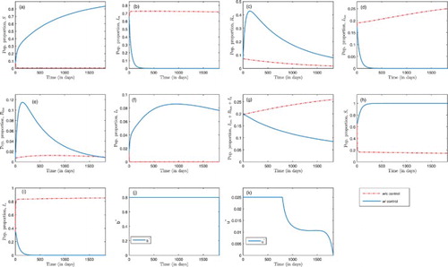
Figure 6. Optimal treatment in the absence of insecticide-treated bed-net coverage, with $B_3=0$, $C_2=0$, $b_{max}=0$. The solid lines represent trajectories in the presence of malaria treatment, but in the absence of insecticide-treated bed-net coverage; the dashed lines represent trajectories in the absence of malaria treatment and insecticide-treated bed-net coverage.

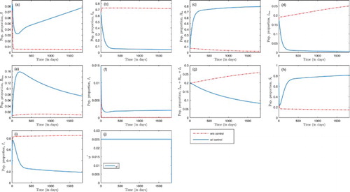
Figure 7. Optimal insecticide-treated bed-net coverage in the absence of treatment, with $A_1=0$, $A_2=0$, $B_1=0$, $B_2=0$, $C_1=0$, $u_{max}=0$. The solid lines represent trajectories in the presence of insecticide-treated bed-net, but in the absence of treatment; the dashed lines represent trajectories in the absence of malaria treatment and insecticide-treated bed-net coverage.

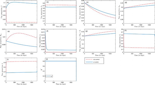
Figure 8. Optimal insecticide-treated bed-net coverage and treatment when: (i) in (a)–(f), $u_{\max }=0.025$, for different values of $b_{\max }$ (i.e. $b_{\max }=0.2,0.75,0.8$ and 0.95); and (ii) in (f)–(j), $b_{\max }=0.25$, for different values of $u_{\max }$ (i.e. $u_{\max }=0.0002,0.005,0.025$ and 0.2). The solid blue lines represent trajectories in the presence of insecticide-treated nets and treatment, the dashed magenta trajectories are insecticide-treated nets only; the broken green trajectories are treatment only; and the red broken lines are without control.

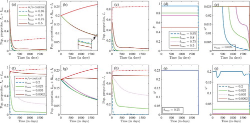
Figure 5 delineates a combination of optimal insecticide-treated bed-net coverage and malaria treatment. The basic reproduction number is ${\mathcal{R}}_0=7.4753$ when b=0 and u=0 (since ${\mathcal{R}}_h=0.9670$ and ${\mathcal{R}}_m=7.4753$). In Figure 5(a), 5(c) and 5(h), more susceptible humans, recovered humans with temporary immunity, and susceptible mosquitoes are observed when both controls are applied than in the absence of such control efforts. Figure 5(b), 5(d) and 5(i) represents malaria-infected humans, humans co-infected with malaria and HIV, and infected mosquitoes, respectively. A rapid decrease in population is observed in the presence of both control efforts than in the absence of such control effort. In Figure 5(e) and 5(f), and in the presence of control, there is a rapid initial increase followed by a decrease for HIV-infected humans with temporary immunity to malaria, and an increase followed by steady decrease in the proportion of humans infected with HIV alone. However, there is a rapid decrease in HIV-infected population in the absence of control as in Figure 5(f). These figures suggest that with optimal treatment and insecticide-treated bed-net coverage, malaria could be contained after 400 days. Without control, HIV prevalence increased from $19.7\mathrm{\%}$ at the beginning to $26\mathrm{\%}$ after 5 years. With this control, HIV infection decreases slowly, and by the end of the fifth year, HIV prevalence dropped from $19.7\mathrm{\%}$ at the beginning of the control period to approximately $8.47\mathrm{\%}$ at the end of the control period. In Figure 5(j) and5(k), the optimal solution for the controls, b and u, are presented. Simulations for our controls suggest a maximum effort for insecticide-treated bed-net coverage, b, for the entire time horizon, and a maximum malaria treatment effort,u, within the first 797 days (approximately 2.2 years), followed by a decrease afterwords.

Figure 6 represents trajectories for humans and mosquitoes in the absence of insecticide-treated bed-net coverage (i.e. $b\left(t\right)=0$), but in the absence/presence of malaria treatment. As malaria treatment is administered (i.e. $u\ge 0$), malaria infection in humans decreases for the first 250 days and remains constant afterwards as shown in Figure 6(b) and 6(d); only 4.9% of the total human population are infected with malaria by the end of the five-year control period. For the mosquito population, there is an initial increase followed by a decrease afterwards as shown in Figure 6(i); by the end of the five years, 18.9% of the mosquito population are infected with malaria. Also, with malaria treatment, HIV infection decreases and prevalence is dropped to 8.15% by the end of the control period as shown in Figure 6(g). The optimal solution for malaria treatment, u, is at the maximum effort throughout the entire control period.

In Figure 7, the dynamics of human and mosquito populations are presented in the absence of malaria treatment, but in the absence/presence of insecticide-treated bed-net coverage. With insecticide-treated nets as the only control measure, malaria infection is at 38% in the mosquito population throughout the control period as delineated in Figure 7(i). In the human population, there is a slight decrease in proportion of malaria-only infection (Figure 7(b)) and a slight decrease in malaria-HIV co-infection (Figure 7(d)) when treated nets are used compared to the case without control, but the infection remains high throughout the control period. HIV prevalence increases to 23% within the entire time horizon of control, from a 19.7% initial prevalence, which is a slight decrease compared to 26% prevalence in the absence of control, at the end of the fifth year, as in Figure 7(g). The effort of insecticide-treated bed-net coverage, b, is at the maximum level throughout the control period as depicted in Figure 7(j).

The value of the objective functional (21(21) $b^{\ast }\left(t\right)=min\left\{b_{max},max\left\{0,\frac{\mathrm{\Psi }\left(t\right)}{2C_2}\right\}\right\}\text{and}{u}^{\ast }\left(t\right)=min\left\{u_{max},max\left\{0,\frac{\mathrm{\Phi }\left(t\right)}{2C_1}\right\}\right\},$(21) ) is computed at the optimal solution for the strategies presented in Figures 5–7. The value of the objective functional or cost at the optimal solution is 10,416,998 when a combination of malaria treatment and insecticide-treated nets are used (Figure 5); 144,779,417 when only malaria treatment is used (Figure 6); and 129,660,019 when only insecticide-treated nets are used (Figure 7). Thus, optimal combination of malaria treatment and insecticide-treated bed-net control has the lowest cost, and this cost is reduced by 92.80% compared to treatment-only control and by 91.96% compared to the treated bed-net control only. The optimal combination of controls eliminates malaria infection and reduces HIV infection prevalence to 8.47% as shown in Figure 5. The optimal malaria treatment control reduces malaria infection to $4.9\mathrm{\%}$ in humans and HIV infection to $8.15\mathrm{\%}$ by the end of the control period. However, it has a significantly higher cost compared to optimal combination of malaria treatment and insecticide-treated bed-net control.

In Figure 8(a)–(e), the maximum treatment control rate is $u_{max}=0.025$, and we consider different values of the maximum treated bed-net coverage, $b_{max}$. During the control period, malaria is eliminated when maximum bed-net coverage is at $b_{max}=0.95,0.8$ and 0.75. However, when $b_{max}=0.5$, the proportion of malaria-infected humans is significantly reduced but malaria is not eliminated as delineated in Figure 8(a) and8(c). The optimal effort in treated bed-net coverage is at the upper bound for all values of $b_{max}$, Figure 8(e). In Figure 8(e), the optimal malaria treatment is: (i) at the maximum level for the first 485 days followed by a decrease afterward for $b_{\max }=0.95$; (ii) at the maximum level for the first 800 days followed by a decrease to zero when $b_{max}=0.8$; (iii) at the maximum level for the first 1, 150 days (or three years and two months) followed by a decrease to zero when $b_{max}=0.75$; (iv) at the maximum level throughout the control period when $b_{\max }=0.5$. Thus, a decrease in insecticide-treated bed-net coverage results in a longer control period at the maximum level of the respective treatment control. At these levels of bed-net coverage, HIV prevalence is at 8.50%, 8.48%, 8.46% and 8.39% when $b_{max}=0.95$, $b_{max}=0.8$, $b_{\max }=0.75$ and $b_{max}=0.5$ respectively. The value of the objective functional or cost is 8,743,136 when $b_{max}=0.95$; 10,445,533 when $b_{max}=0.8$; 11,473,140, $b_{max}=0.75$; and 36,314,750 when $b_{max}=0.5$. Thus, when malaria treatment rate is fixed at u=0.025, increasing the coverage of treated bed-net management is vital in eliminating/reducing malaria infection, and there is a slight percentage increase in HIV prevalence as the bed-net coverage increases but the cost implementing the control is significantly reduced as treated bed-net coverage increases.

Finally, in Figure 8(f)–(j), the maximum treated bed-net coverage is at a lower coverage of $b_{max}=0.25$ and we considered various values of maximum malaria treatment rate. That is, $u\in \{0.0002,0.005,0.025,0.2\}$. Malaria infection is eliminated only when $u_{max}=0.2$, that is, for a higher treatment rate. Figure 8(f) and 8(h) represents the proportion of malaria-infected humans and mosquitoes, respectively, which increase as maximum malaria treatment rate decreases. The maximum treated bed-net coverage is at maximum level within the entire control period as shown in Figure 8(i). The optimal malaria treatment is at maximum treatment rate for all $u_{max}$, except for $u_{max}=0.2$ as portrayed in Figure 8(j). In the presence of control, HIV prevalence is at $8.42\mathrm{\%}$, $8.17\mathrm{\%}$, $8.54\mathrm{\%}$ and $20.2\mathrm{\%}$ when $u_{max}=0.2$, $u_{max}=0.025$, $u_{max}=0.005$ and $u_{max}=0.0002$ respectively. The value of the objective functional or cost is at 6,783,926 when $u_{max}=0.2$; 78,224,817 when $u_{max}=0.025$; 208,322,647 when $u_{\max }=0.005$; and 333,968,948 when $u_{max}=0.0002$. From Figure 8, we conclude that in an environment with limited resources for malaria treatment (i.e. at a fixed maximum treatment) rate $u_{max}=0.025$, malaria is eliminated and HIV prevalence is reduced with minimum cost when treated bed-net coverage is high (i.e. $b_{max}=0.95$). On the other hand, in an environment with limited resources for treated bed-net coverage with a maximum bed-net coverage as low as $b_{max}=0.25$, increasing malaria treatment rate to $u_{max}=0.2$ is crucial in eliminating malaria and reducing HIV prevalence with minimum cost.

Figure  5–8 suggests that in malaria-HIV endemic areas, an optimal malaria treatment and treated bed-net usage is useful not only to eliminate malaria, but also to reduce HIV prevalence in the environment.

5. Conclusion

We proposed a mathematical model for malaria-HIV co-infection transmission and control in which malaria treatment and insecticide-treated bed-net controls are incorporated. We derived an expression for the basic reproduction number, showed the existence of a unique HIV-only boundary equilibrium, and derived conditions for the existence of either a unique malaria-only boundary equilibrium or existence of two malaria-only boundary equilibria or no malaria-only boundary equilibrium.

Also, using the centre of manifold theory [4], we analysed the possibility of backward bifurcation, where a locally asymptotically stable DFE coexist with a locally asymptotically stable endemic equilibrium. We showed that the occurrence of backward bifurcation is influenced by the disease-induced mortality, the bed-net coverage and the malaria treatment parameters. The influence of the two control parameters, bed-net coverage, b, and malaria treatment, u, are explored numerically in Figures 2–4. The numerical simulations suggest that malaria treatment and insecticide-treated nets are important in eliminating malaria and HIV in the long run at equilibrium.

We formulated an optimal control problem for the model system (1(1) $\begin{array}{rl}\dot{S}& ={\mathrm{\Lambda }}_h+\sigma u{I}_m+\rho R_m-({\lambda }_h+{\omega }_h+{\alpha }_1{\omega }_{hm}+\mu )S\\ {\dot{I}}_m& ={\lambda }_{h}S-({\omega }_h+{\alpha }_2{\omega }_{hm}+\gamma +u+{\mu }_m+\mu )I_m\\ {\dot{R}}_m& =(\gamma +(1-\sigma \left)u\right)I_m-({\omega }_h+{\alpha }_1{\omega }_{hm}+\rho +\mu )R_m\\ {\dot{I}}_{hm}& =({\omega }_h+{\alpha }_2{\omega }_{hm})I_m+{\alpha }_3{\lambda }_h{I}_h-({\kappa }_1\gamma +u+{\mu }_{hm}+\mu )I_{hm}\\ {\dot{R}}_{hm}& =\left(\right(1-\sigma )u+{\kappa }_1\gamma )I_{hm}+({\omega }_h+{\alpha }_1{\omega }_{hm})R_m-({\kappa }_2\rho +{\mu }_h+\mu )R_{hm}\\ {\dot{I}}_h& =\sigma u{I}_{hm}+{\kappa }_2\rho R_{hm}+({\omega }_h+{\alpha }_1{\omega }_{hm})S-({\alpha }_3{\lambda }_h+{\mu }_h+\mu )I_h\\ {\dot{S}}_v& ={\mathrm{\Lambda }}_v-({\lambda }_v^m+{\alpha }_4{\lambda }_v^{hm}+{\mu }_v(b\left)\right)S_v\\ {\dot{I}}_v& =({\lambda }_v^m+{\alpha }_4{\lambda }_v^{hm})S_v-{\mu }_v\left(b\right)I_v,\end{array}$(1) ) to investigate optimal malaria treatment and insecticide-treated bed-net control strategies that reduce/eliminate malaria and HIV in shorter control period of time. Numerical simulations of the optimal control suggest that in some cases implementing optimal malaria treatment and treated bed-net control eliminates malaria in the population and reduce HIV prevalence significantly from $26\mathrm{\%}$ in the absence of control to $8.47\mathrm{\%}$ in the presence of control. Even though HIV and malaria have different transmission mechanisms, our results suggest that, if malaria is not controlled, HIV will be endemic (even if ${\mathcal{R}}_h<1$); this is due to the amplification effect caused by co-infection, which is incorporated in the model. However, high bed-net coverage or high malaria treatment rate (or both) will significantly minimize malaria-HIV co-infection and the reduction in co-infection (or elimination of co-infection) will result in reduction or even eradication of HIV prevalence, since we considered ${\mathcal{R}}_h<1$. These results are consistent with the results in [9, 10] in that amplification effect is a driving force to maintain HIV endemic/epidemic if malaria is not controlled. In [23], the authors studied a deterministic model of HIV and malaria, and established stability results for sub-models and full model. Also, the existence of backward bifurcation is established analytical and numerically. Barley et al. [17] studied an SI model for malaria and malaria-HIV co-infection, and established local stability results, together with some sensitivity analysis results. Most recently, Nyabadza et al. [25] studied the effect of treatment on HIV-malaria co-infection dynamics. None of these authors studied the use of insecticide-treated nets in their co-infection models. In our model, we have incorporated insecticide-treated nets and malaria treatment, and have formulated and analysed an optimal control problem. To the best of our knowledge, the use of optimal control theory in malaria and HIV co-infection model incorporating insecticide-treated nets is novel.

Our model can be extended by incorporating preventive and therapeutic strategies for HIV such as anti-retroviral therapy, the use of condoms as well as other malaria control strategies, such as vector control, IPT in children and pregnant women. Also, the model can be strengthened by incorporating two HIV-infectious classes, HIV-infected humans without AIDS symptoms and those with AIDS symptoms, as well as by incorporating exposed classes for malaria in both humans and mosquitoes.

Acknowledgments

Eric Numfor would like to acknowledge support from the College of Science and Mathematics at Augusta University, and Jemal Mohammed-Awel would like to acknowledge the faculty seed grant from Valdosta State University, Georgia. The authors acknowledge publication support from Valdosta State University Mathematics & Computer Science Department. Jemal Mohammed-Awel acknowledges the support of the National Institute for Mathematical and Biological Synthesis (NIMBios) Sabbatical Fellowship program.

Disclosure statement

No potential conflict of interest was reported by the authors.

Appendix 1. More theorems and some proofs

Theorem.1

(Catillo-Chavez and Song)

Let $\mathrm{d}x/\mathrm{d}t=f(x,\phi )$ refer to the general system of ordinary differential equations, where $f:R^n\times R\to R^n,$ $f\in {\mathbb{C}}^2(R^n\times R),$ and φ is a parameter. Without loss of generality, let 0 be an equilibrium of the system so that $f(0,\phi )=0$ for all φ. Assume

1. $A=D_{x}f(0,0),$ that is, the Jacobian of the system evaluated at the zero equilibrium, with $\phi =0$. Zero is a simple eigenvalue of A and all other eigenvalues of A have negative real parts.

2. Matrix A has a non-negative right eigenvector w and a left eigenvector v corresponding to the zero eigenvalue.

Let $f_k$ be the kth component of f and $\begin{array}{rl}{a}_0& =\sum _{k,i,j=1}^n{v}_k{w}_i{w}_j\frac{{\mathrm{\partial }}^2{f}_k}{\mathrm{\partial }{x}_i\mathrm{\partial }{x}_j}(0,0)\\ b_0& =\sum _{k,i=1}^n{v}_k{w}_i\frac{{\mathrm{\partial }}^2{f}_k}{\mathrm{\partial }{x}_i\mathrm{\partial }\phi }(0,0).\end{array}$ Then, the local dynamics of the system are completely determined by the signs of $a_0$ and $b_0$. In particular, if $a_0$ and $b_0>0,$ the bifurcation at $\phi =0$ is subcritical $($ i.e. backward $)$.

Remark.2.

The condition in assumption (2) of Theorem A.1 that the right eigenvector w be positive is not necessary. If $x_0$ denotes the equilibrium, we only need $w\left(j\right)>0$ whenever $x_0\left(j\right)=0$. If $x_0\left(j\right)>0$, then $w\left(j\right)$ need not be positive.

Appendix 2. Tables

Table A.1. Parameters of model (1(1) $\begin{array}{rl}\dot{S}& ={\mathrm{\Lambda }}_h+\sigma u{I}_m+\rho R_m-({\lambda }_h+{\omega }_h+{\alpha }_1{\omega }_{hm}+\mu )S\\ {\dot{I}}_m& ={\lambda }_{h}S-({\omega }_h+{\alpha }_2{\omega }_{hm}+\gamma +u+{\mu }_m+\mu )I_m\\ {\dot{R}}_m& =(\gamma +(1-\sigma \left)u\right)I_m-({\omega }_h+{\alpha }_1{\omega }_{hm}+\rho +\mu )R_m\\ {\dot{I}}_{hm}& =({\omega }_h+{\alpha }_2{\omega }_{hm})I_m+{\alpha }_3{\lambda }_h{I}_h-({\kappa }_1\gamma +u+{\mu }_{hm}+\mu )I_{hm}\\ {\dot{R}}_{hm}& =\left(\right(1-\sigma )u+{\kappa }_1\gamma )I_{hm}+({\omega }_h+{\alpha }_1{\omega }_{hm})R_m-({\kappa }_2\rho +{\mu }_h+\mu )R_{hm}\\ {\dot{I}}_h& =\sigma u{I}_{hm}+{\kappa }_2\rho R_{hm}+({\omega }_h+{\alpha }_1{\omega }_{hm})S-({\alpha }_3{\lambda }_h+{\mu }_h+\mu )I_h\\ {\dot{S}}_v& ={\mathrm{\Lambda }}_v-({\lambda }_v^m+{\alpha }_4{\lambda }_v^{hm}+{\mu }_v(b\left)\right)S_v\\ {\dot{I}}_v& =({\lambda }_v^m+{\alpha }_4{\lambda }_v^{hm})S_v-{\mu }_v\left(b\right)I_v,\end{array}$(1) ). The baseline parameter values and range of values are drawn from [17, 24].

Param.	Description	Baseline value	Dimensions
${\mathrm{\Lambda }}_h$	Human recruitment rate	${10}^4/(55\ast 365)$	Human × day^−1
${\mathrm{\Lambda }}_v$	Mosquito recruitment rate	${10}^4/14$	Mosquito × day^−1
${\beta }_h$	Rate of HIV transmission	Variable	Day^−1
u	Rate of treatment of malaria infection	Variable	Day^−1
σ	Proportion of treated infectious humans who recover without acquiring immunity	4/10	Dimensionless
γ	Per capita recovery rate from malaria	$1\times {10}^{-5}$	Day^−1
ρ	Rate at which temporary immune recovered humans lose immunity	$1/(5\times 365)$	Day^−1
${\kappa }_1$	Reduction factor of the recovery rate of the Malaria-HIV co-infection from malaria	1/2	Day^−1
${\kappa }_2$	Amplification factor of the rate of loss of immunity of Malaria of the $R_{hm}$ class	2	Day^−1
${\mu }_h$	Mortality rate of humans infected with HIV	$2.3\times {10}^{-4}$	Day^−1
${\mu }_m$	Mortality rate of humans infected with malaria	$3.354\times {10}^{-3}$	Day^−1
${\mu }_{hm}$	Mortality rate of humans infected with HIV and malaria	$1.4\times {10}^{-3}$	Day^−1
${\mu }_{v0}$	Mosquito daily mortality rate	1/14	Day^−1
${\mu }_{v1}$	Additional mortality rate due to insecticide-treated bed-net	1/14	Day^−1
μ	Per capita natural mortality rate of humans	$5.7078\times {10}^{-5}$	Day^−1
$p_{vh}$	Disease transmission probability from infectious mosquitoes to susceptible humans	$22/{10}^3$	Dimensionless
$p_{hv}$	Disease transmission probability from infectious humans to susceptible mosquitoes	$48/{10}^2$	Dimensionless
${\alpha }_i$	Amplification factor	4	Dimensionless
b	Insecticide-treated bed-net coverage	$0\le b\le 1$	Dimensionless
${\beta }_{\min }$	Minimum mosquito biting rate	$1\times {10}^{-2}$	Human × mosquito^−1 × day^−1
${\beta }_{\max }$	Maximum mosquito biting rate	$0.5\in [0,1]$	Human × mosquito^−1 × day^−1

Table A.2. Sensitivity indices of ${\mathcal{R}}_m$ for HIV-free sub-model of (1(1) $\begin{array}{rl}\dot{S}& ={\mathrm{\Lambda }}_h+\sigma u{I}_m+\rho R_m-({\lambda }_h+{\omega }_h+{\alpha }_1{\omega }_{hm}+\mu )S\\ {\dot{I}}_m& ={\lambda }_{h}S-({\omega }_h+{\alpha }_2{\omega }_{hm}+\gamma +u+{\mu }_m+\mu )I_m\\ {\dot{R}}_m& =(\gamma +(1-\sigma \left)u\right)I_m-({\omega }_h+{\alpha }_1{\omega }_{hm}+\rho +\mu )R_m\\ {\dot{I}}_{hm}& =({\omega }_h+{\alpha }_2{\omega }_{hm})I_m+{\alpha }_3{\lambda }_h{I}_h-({\kappa }_1\gamma +u+{\mu }_{hm}+\mu )I_{hm}\\ {\dot{R}}_{hm}& =\left(\right(1-\sigma )u+{\kappa }_1\gamma )I_{hm}+({\omega }_h+{\alpha }_1{\omega }_{hm})R_m-({\kappa }_2\rho +{\mu }_h+\mu )R_{hm}\\ {\dot{I}}_h& =\sigma u{I}_{hm}+{\kappa }_2\rho R_{hm}+({\omega }_h+{\alpha }_1{\omega }_{hm})S-({\alpha }_3{\lambda }_h+{\mu }_h+\mu )I_h\\ {\dot{S}}_v& ={\mathrm{\Lambda }}_v-({\lambda }_v^m+{\alpha }_4{\lambda }_v^{hm}+{\mu }_v(b\left)\right)S_v\\ {\dot{I}}_v& =({\lambda }_v^m+{\alpha }_4{\lambda }_v^{hm})S_v-{\mu }_v\left(b\right)I_v,\end{array}$(1) ).

Parameter	Sensitivity index	Parameter	Sensitivity index	Parameter	Sensitivity index
${\mathrm{\Lambda }}_h$	$-0.5000$	γ	$-0.0021$	${\beta }_{\min }$	$+0.0358$
${\mathrm{\Lambda }}_v$	$+0.5000$	u	$-0.4145$	${\mu }_{v0}$	$-0.6061$
$p_{hv}$	$+0.5000$	b	$-2.1488$	${\mu }_{v1}$	$-0.3939$
$p_{vh}$	$+0.5000$	${\beta }_{\max }$	$+0.9642$	${\mu }_m$	$-0.0716$
μ	$+0.4882$

Table A.3. Weight constants and maximum malaria treatment.

Parameter	$A_1$	$A_2$	$A_3$	$B_1$	$B_2$	$B_3$	$C_1$	$C_2$
Value	10	$2A_1$	30	2.25	2 $B_1$	4	50	50

Appendix 3. Adjoint equations

(A1) $\begin{array}{rl}\frac{\mathrm{d}{\xi }_1}{\mathrm{d}t}& =-(a_1{\tilde{\lambda }}_h+a_1{\omega }_h+a_1{\alpha }_1{\omega }_{hm}-\mu ){\xi }_1+(a_1{\tilde{\lambda }}_h-d_2{I}_m){\xi }_2-d_1{R}_m{\xi }_3+(d_2{I}_m+{\alpha }_3{d}_3{I}_h){\xi }_4\\ & +d_1{R}_m{\xi }_5+(a_1{\omega }_h+a_1{\alpha }_1{\omega }_{hm}-{\alpha }_3{d}_3{I}_h){\xi }_6-d_4{S}_v{\xi }_7+d_4{S}_v{\xi }_8-B_{3}b,\\ \frac{\mathrm{d}{\xi }_2}{\mathrm{d}t}& =(-\sigma u-d_{3}S-d_{1}S){\xi }_1+(d_{3}S-a_2{\omega }_h-a_2{\alpha }_2{\omega }_{hm}+K_0){\xi }_2\\ & -(K_1+d_1{R}_m){\xi }_3+(a_2{\omega }_h+a_2{\alpha }_2{\omega }_{hm}+{\alpha }_3{d}_3{I}_h){\xi }_4+d_1{R}_m{\xi }_5\\ & +(d_{1}S-{\alpha }_3{d}_3{I}_h){\xi }_6-d_5{S}_v{\xi }_7+d_5{S}_v{\xi }_8-B_{1}u-B_{3}b-A_1,\\ \frac{\mathrm{d}{\xi }_3}{\mathrm{d}t}& =-(\rho +d_{3}S+d_{1}S){\xi }_1+(d_{3}S-d_1{I}_m)){\xi }_2+(-a_3{\omega }_h-{\alpha }_1{a}_3{\omega }_{hm}+K_2){\xi }_3\\ & +(d_2{I}_m+{\alpha }_3{d}_3{I}_h){\xi }_4+(a_3{\omega }_h+{\alpha }_1{a}_3{\omega }_{hm})){\xi }_5+(d_{1}S-{\alpha }_3{d}_3{I}_h){\xi }_6\\ & -d_4{\xi }_7+d_4{\xi }_8-B_{3}b,\\ \frac{\mathrm{d}{\xi }_4}{\mathrm{d}t}& =-(d_3+e_3)S{\xi }_1+(d_3-e_2)S{\xi }_2-({\alpha }_1{e}_3{\beta }_h{a}_4+e_3{\omega }_h){\xi }_3\\ & +(e_3{I}_m+{\alpha }_3{d}_3{I}_h+K_3){\xi }_4+({\alpha }_1{\beta }_h{e}_3{a}_4+{\omega }_h{e}_3+K_4){\xi }_5\\ & +(e_{1}S-{\alpha }_3{d}_3{I}_h-\sigma u){\xi }_6-e_4{S}_v{\xi }_7+e_4{S}_v{\xi }_8-B_{2}u-B_{3}b-A_2\\ \frac{\mathrm{d}{\xi }_5}{\mathrm{d}t}& =-\left(d_{3}S+\frac{{\alpha }_1{\omega }_{hm}S}{N}-\frac{a_5{\beta }_{h}S}{N}\right){\xi }_1+\left(d_{3}S+\frac{a_5{\beta }_h{I}_m}{N}-\frac{{\alpha }_2{\omega }_{hm}{I}_m}{N}\right){\xi }_2\\ & +(-{\alpha }_1{e}_3{\omega }_{hm}+e_3{a}_5{\beta }_h){\xi }_3+\left(-\frac{a_5{\beta }_h{I}_m}{N}+\frac{{\alpha }_2{\omega }_{hm}{I}_m}{N}+{\alpha }_3{d}_3{I}_h\right){\xi }_4\\ & +({\alpha }_1{e}_3{\omega }_{hm}-a_5{e}_3{\beta }_h+K_5){\xi }_5-\left({\kappa }_2\rho +\frac{a_5{\beta }_{h}S}{N}-\frac{{\alpha }_1{\omega }_{hm}S}{N}+{\alpha }_3{d}_3{I}_h\right){\xi }_6\\ & -d_4{S}_v{\xi }_7+d_4{S}_v{\xi }_8-B_{3}b,\\ \frac{\mathrm{d}{\xi }_6}{\mathrm{d}t}& =-\left(d_{3}S-\frac{a_5{\beta }_{h}S}{N}+\frac{{\alpha }_1{\omega }_{hm}S}{N}\right){\xi }_1+\left(d_{3}S+\frac{a_5{\beta }_h{I}_m}{N}-\frac{{\alpha }_2{\omega }_{hm}{I}_m}{N}\right){\xi }_2\\ & -\left({\alpha }_1{e}_3{\omega }_{hm}-\frac{a_5{\beta }_h{R}_m}{N}\right){\xi }_3+\left(-\frac{a_5{\beta }_h{I}_m}{N}+\frac{{\alpha }_2{\omega }_{hm}{I}_m}{N}+{\alpha }_3{a}_6{\tilde{\lambda }}_h\right){\xi }_4\\ & +({\alpha }_1{e}_3{\omega }_{hm}-e_3{a}_5{\beta }_h){\xi }_5+\left(-\frac{a_5{\beta }_{h}S}{N}+\frac{{\alpha }_1{\omega }_{hm}S}{N}-{\alpha }_3{a}_6{\tilde{\lambda }}_h)+K_6\right){\xi }_6\\ & -d_4{S}_v{\xi }_7+d_4{S}_v{\xi }_8-B_{3}b,\\ \frac{\mathrm{d}{\xi }_7}{\mathrm{d}t}& =({\tilde{\lambda }}_v^m+{\alpha }_4{\tilde{\lambda }}_v^{hm}+{\mu }_v(b\left(t\right)\left)\right){\xi }_7-({\tilde{\lambda }}_v^m+{\alpha }_4{\tilde{\lambda }}_v^{hm}){\xi }_8\\ \frac{\mathrm{d}{\xi }_8}{\mathrm{d}t}& =\frac{{\rho }_{vh}\beta \left(b\right(t\left)\right)S}{N}{\xi }_1-\frac{{\rho }_{vh}\beta \left(b\right(t\left)\right)S}{N}{\xi }_2-\frac{{\alpha }_3{\rho }_{vh}\beta \left(b\right(t\left)\right)I_h}{N}{\xi }_4+\frac{{\alpha }_3{\rho }_{vh}\beta \left(b\right(t\left)\right)I_h}{N}{\xi }_6\\ & +{\mu }_v\left(b\right(t\left)\right){\xi }_8-A_3,\end{array}$(A1) with transversality conditions (A2) ${\xi }_j\left(T\right)=0,\text{for}j=1,2,\dots ,8,$(A2) where $\begin{array}{rl}{a}_1& =\frac{S}{N}-1a_2=\frac{I_m}{N}-1a_3=\frac{R_m}{N}-1a_4=\frac{I_{hm}}{N}-1a_5=1-\frac{I_m+R_{hm}}{N}\\ a_6& =\frac{I_h}{N}-1d_1=\frac{{\omega }_h+{\alpha }_1{\omega }_{hm}}{N}{d}_2=\frac{{\omega }_h+{\alpha }_2{\omega }_{hm}}{N}{d}_3=\frac{{\tilde{\lambda }}_h}{N}{d}_4=\frac{{\tilde{\lambda }}_v^m+{\alpha }_4{\tilde{\lambda }}_v^{hm}}{N}\\ d_5& =\frac{a_2{p}_{hv}\beta \left(b\right)}{N}+\frac{{\alpha }_4{\tilde{\lambda }}_v^{hm}}{N}{e}_1=\frac{{\omega }_h+{\alpha }_1{\beta }_h{a}_4}{N}{e}_2=\frac{{\omega }_h+{\alpha }_2{\beta }_h{a}_4}{N}{e}_3=\frac{R_m}{N}\\ e_4& =\frac{{\tilde{\lambda }}_v^m}{N}+\frac{{\alpha }_4{p}_{hv}\beta \left(b\right)a_4}{N}.\end{array}$