Characteristics of an epidemic outbreak with a large initial infection size

ABSTRACT

A deterministic model proposed in previous literatures to approximate the well-known Richards model is investigated. However, the model assumption of small initial value for infection size is released in the current manuscript. Taking the advantage of the closed form of solutions, we establish the epidemic characteristics of disease transmission: the outbreak size, the peak size and the turning point for the cumulative infected cases. It is shown that the usual disease outbreak threshold condition (the basic reproduction number ${\mathcal{R}}_0$ is greater than unity) fails to fully guarantee the existence of peaking time and turning point when the initial infection size is not relatively small. The epidemic characteristics not only depend on ${\mathcal{R}}_0$ but also on another index, the net reproduction number ${\mathcal{R}}_0^{\ast }$.

KEYWORDS:

• Epidemic characteristics
• outbreak size
• turning point
• peak size
• large initial infection size

AMS SUBJECT CLASSIFICATION:

• 92D30
• 92B05

1. Introduction

The Richards model [14] $\frac{\mathrm{d}C\left(t\right)}{\mathrm{d}t}=rC\left(t\right)\left[1-{\left(\frac{C\left(t\right)}{K_0}\right)}^a\right],$ also known as the theta-logistic model [15], was initially formulated as an extension to the logistic model in order to investigate the ecological population growth. Since last decade, it has been widely employed to fit epidemic data. Unlike models with several compartments commonly used to predict the disease spread, the Richards model considers only the cumulative infective population size with saturation in growth as the outbreak progresses, caused by decreases in recruitment because of attempts to avoid contacts (e.g. wearing facemask) and implementation of control measures. In this single equation, $C\left(t\right)$ represents the cumulative infected cases at moment t, $K_0$ is the carrying capacity or total case number (maximum case number), r is the per-capita growth rate of the infected population and a is the exponent of deviation from the standard logistic curve which makes the model much more flexible: a>1 (or a<1) signifies that the cumulative number of infection grows faster (or slower) than that predicted by the logistic growth model. The solution to the Richards model can be explicitly expressed by $C\left(t\right)=K_0[1+a{e}^{-ar(t-t_{\mathrm{T}})}{]}^{-1/a}$ with $t_{\mathrm{T}}$ being the turning point defined as the time when the second derivative of $C\left(t\right)$ equals zero, or equivalently, when $C\left(t\right)$ takes the value $K_0(1+a{)}^{-1/a}$ [17]. For more details about the Richards model, we refer the reader to the study [4].

Some epidemic pattern suggests a single S-shaped curve for the cumulative cases, which is consistent with the solution of the Richards model. Therefore, the Richards model is used to fit the single-phase severe acute respiratory syndrome (SARS) outbreaks in Hong Kong and Taiwan well [10,19]. Meanwhile, it is also employed to fit the 2005 dengue outbreak in Singapore to study the impact of intervention measures relating to the turning point [11], the weekly reported dengue case data in Havana City to assess the contribution of hurricane to dengue transmission [8] as well as H1N1 [5,9]. The Richards model gives a single S-shaped curve while some epidemic datasets share a multiphase outbreak pattern, such as dengue outbreaks in Taiwan [6]. To fit these multiple-wave patterns, Hsieh and his collaborators proposed a multiphase Richards model [7] and their method was successfully used to fit the multi-wave dengue outbreak in Taiwan [6] and 2003 SARS outbreak in Toronto [7].

This Richards model has made so many successful applications in real-time data fitting and predictions of infection dynamics, although several parameters (e.g. the exponential term) share no clear epidemiological explanation, which poses a puzzle to the community of theoretical epidemiology to find the intrinsic link between the Richards model and well-established deterministic epidemic models, such as the Kermack–McKendrick model. To approximate the Richard model, recently the authors in [17] proposed the following model (1) $\begin{array}{rl}\frac{\mathrm{d}S}{\mathrm{d}t}& =-\beta S\frac{I}{N},\\ \frac{\mathrm{d}I}{\mathrm{d}t}& =\beta S\frac{I}{N}-\delta I,\\ N& =S+I,\end{array}$(1) a modified version of the classical SIR model. The novelty of the model lies on the consideration of the ‘actually at risk’ total population $N\left(t\right)$, which is defined as the eventually infected population, that is, $N\left(t\right)=S\left(t\right)+I\left(t\right)$ is the total number of ‘actually’ vulnerable individuals for the disease transmission at time t [12], $S\left(t\right)$ is the actually at risk susceptibles that will be exposed to the pathogen during the entire epidemic under consideration (at ‘actual’ risk for infection) and $I\left(t\right)$ is the number of infected individuals. In their model, the frequency-dependent disease transmission term $\beta SI/N$ is used, while δ is the removal rate, which refers to all removal forms from the infected individuals due to disease induced death or recovery. In [17], this model is used to illustrate the epidemiological interpretations for parameters in the Richards model, especially the exponent a. The model (1(1) $\begin{array}{rl}\frac{\mathrm{d}S}{\mathrm{d}t}& =-\beta S\frac{I}{N},\\ \frac{\mathrm{d}I}{\mathrm{d}t}& =\beta S\frac{I}{N}-\delta I,\\ N& =S+I,\end{array}$(1) ) is also validated to the datasets for Canada 2009 H1N1 two-stage epidemic outbreak data, two-stage SARS outbreak data in Toronto, Singapore 2005 dengue data, and Taiwan 2003 SARS data and the results are compared with those obtained by the Richards model in terms the turning point and multiple waves/phases. The model (1(1) $\begin{array}{rl}\frac{\mathrm{d}S}{\mathrm{d}t}& =-\beta S\frac{I}{N},\\ \frac{\mathrm{d}I}{\mathrm{d}t}& =\beta S\frac{I}{N}-\delta I,\\ N& =S+I,\end{array}$(1) ) is also adopted to describe the transmission of avian influenza (H7N9) virus among birds [12] and then extended to infer the dynamics of the cumulative number of infected humans due to infection transmitted by infected birds. Fitting the epidemic data for humans, the authors estimated the key parameters in the model system quantifying the bird and human components of an avian influenza epidemic. More recently, this model is used to fit the Ebola outbreak in west Africa [18].

All these previous investigations provide important information on epidemic characteristics and suggestions on epidemic control, but most of them propose an implicit assumption that the disease is initialized by an infinitesimally small proportion of the population, that is, the initial value of infected individuals to the deterministic model is assumed to be very small, which is almost negligible compared to the initial number of susceptibles. However, this underlying assumption for the deterministic model may be unappropriate in some scenarios as argued in [13]. For example, a discrete formulation for disease spread is vital at the initial contamination stage of an epidemic outbreak when the number of infectives is small [16]. In this case, the randomness should be carefully accounted, which can be described by a stochastic process, such as the model in [16] and references therein. In other words, the evolution of an epidemic outbreak in an isolated population can be split into two stages: a stochastic Markov process describing the initial contamination and a linked deterministic dynamical system with random initial conditions for the continued development of the outbreak [16]. Motivated by this, we assume the initial distribution of infectives $I\left(0\right)$ to be not negligible compared with the size of susceptibles. Another reason is related to a late surveillance programme which provides large initial infection value.

In this work, we are going to release the assumption of small initial number of infectious individuals and assume its size can be random. Under this released assumption, we will investigate the final size relationship of the epidemic and predict the real-time number and the peak time of infected individuals. In particular, we are going to figure out the time when the inflection of the cumulative case curve occurs (the turning point), i.e. the moment when a rapid increase in case numbers is replaced by a slower increase and this inflection point indicates the moment when the rate of increases in numbers of cumulative cases reaches its maximum. It is shown that the usual disease outbreak threshold condition (the basic reproduction number is greater than unity) fails to guarantee the existence of peaking time and turning point.

The remaining part of this paper starts from solving the model system to obtain a closed form of solutions, based on which the final size, peak time and turning point are discussed. The conclusion and discussion are given in the last section.

2. Theoretical analysis

We can rewrite the model system (1(1) $\begin{array}{rl}\frac{\mathrm{d}S}{\mathrm{d}t}& =-\beta S\frac{I}{N},\\ \frac{\mathrm{d}I}{\mathrm{d}t}& =\beta S\frac{I}{N}-\delta I,\\ N& =S+I,\end{array}$(1) ) into (2) $\begin{array}{rl}\frac{\mathrm{d}S}{\mathrm{d}t}& =-\beta S\frac{I}{N},\\ \frac{\mathrm{d}I}{\mathrm{d}t}& =\beta S\frac{I}{N}-\delta I,\\ \frac{\mathrm{d}N}{\mathrm{d}t}& =-\delta I,\end{array}$(2) with initial condition $S\left(0\right)=S_0>0$, $I\left(0\right)=I_0>0$, and $N\left(0\right)=N_0=S_0+I_0$. To investigate the characteristics of the epidemic pattern, we start from solving the system directly to obtain a closed form of solutions in terms of the initial values as well as model parameters.

2.1. Explicit solutions

The first and last equations of (2(2) $\begin{array}{rl}\frac{\mathrm{d}S}{\mathrm{d}t}& =-\beta S\frac{I}{N},\\ \frac{\mathrm{d}I}{\mathrm{d}t}& =\beta S\frac{I}{N}-\delta I,\\ \frac{\mathrm{d}N}{\mathrm{d}t}& =-\delta I,\end{array}$(2) ) give $\mathrm{d}S/\mathrm{d}N=\beta /\delta \cdot S/N$ which indicates (3) $S\left(t\right)=S_0{\left(\frac{N\left(t\right)}{N_0}\right)}^{\beta /\delta }.$(3)

Now we solve the system for two different cases: $\beta =\delta$ and $\beta \ne \delta$.

When $\beta =\delta$, the equality (3(3) $S\left(t\right)=S_0{\left(\frac{N\left(t\right)}{N_0}\right)}^{\beta /\delta }.$(3) ) implies $S\left(t\right)/S_0=N\left(t\right)/N_0$. Since $N\left(t\right)=S\left(t\right)+I\left(t\right)$ for all $t\ge 0$, we have (4) $\frac{S\left(t\right)}{S_0}=\frac{I\left(t\right)}{I_0}=\frac{N\left(t\right)}{N_0}.$(4) Therefore $I\left(t\right)=I_{0}N\left(t\right)/N_0$ and the last equation of (2(2) $\begin{array}{rl}\frac{\mathrm{d}S}{\mathrm{d}t}& =-\beta S\frac{I}{N},\\ \frac{\mathrm{d}I}{\mathrm{d}t}& =\beta S\frac{I}{N}-\delta I,\\ \frac{\mathrm{d}N}{\mathrm{d}t}& =-\delta I,\end{array}$(2) ) reads $\mathrm{d}N/\mathrm{d}t=-\delta I_{0}N\left(t\right)/N_0$, from which we obtain $N\left(t\right)=N_0{e}^{-\delta I_0/N_{0}t}.$ Using the relationship (4(4) $\frac{S\left(t\right)}{S_0}=\frac{I\left(t\right)}{I_0}=\frac{N\left(t\right)}{N_0}.$(4) ), we can express the solution into (5) $S\left(t\right)=S_0\frac{N}{N_0}=S_0{e}^{-\delta I_0/N_{0}t},I\left(t\right)=I_0\frac{N}{N_0}=I_0{e}^{-\delta I_0/N_{0}t}.$(5)

When $\beta \ne \delta$, denote $K=N_0^{\beta /(\beta -\delta )}{S}_0^{-\delta /(\beta -\delta )}$, which is a constant determined by the initial value and intrinsic coefficients. Note that $K>N_0$ when $\beta >\delta$ while $K<N_0$ when $\beta <\delta$. In this case, Equation (3(3) $S\left(t\right)=S_0{\left(\frac{N\left(t\right)}{N_0}\right)}^{\beta /\delta }.$(3) ) can be written as (6) $S\left(t\right)=K{\left(\frac{N\left(t\right)}{K}\right)}^{\beta /\delta }.$(6)

Substituting Equation (6(6) $S\left(t\right)=K{\left(\frac{N\left(t\right)}{K}\right)}^{\beta /\delta }.$(6) ) into $I\left(t\right)=N\left(t\right)-S\left(t\right)$, we have (7) $I\left(t\right)=N\left(t\right)\left[1-{\left(\frac{N\left(t\right)}{K}\right)}^{\beta /\delta -1}\right],$(7) and correspondingly, the N-equation in Equation (2(2) $\begin{array}{rl}\frac{\mathrm{d}S}{\mathrm{d}t}& =-\beta S\frac{I}{N},\\ \frac{\mathrm{d}I}{\mathrm{d}t}& =\beta S\frac{I}{N}-\delta I,\\ \frac{\mathrm{d}N}{\mathrm{d}t}& =-\delta I,\end{array}$(2) ) becomes (8) $\frac{\mathrm{d}N}{\mathrm{d}t}=-\delta I\left(t\right)=-\delta N\left(t\right)\left[1-{\left(\frac{N\left(t\right)}{K}\right)}^{\beta /\delta -1}\right].$(8) Since $\beta \ne \delta$, Equation (8(8) $\frac{\mathrm{d}N}{\mathrm{d}t}=-\delta I\left(t\right)=-\delta N\left(t\right)\left[1-{\left(\frac{N\left(t\right)}{K}\right)}^{\beta /\delta -1}\right].$(8) ) takes the form of a Bernoulli equation (also in the form of Richards equation whose solution can be solved) and its solution can be explicitly obtained as $N\left(t\right)=\frac{K}{{\left\{1+\left[{\left(\frac{K}{N_0}\right)}^{(\beta -\delta )/\delta }-1\right]e^{(\beta -\delta )t}\right\}}^{\delta /(\beta -\delta )}}.$

Since $K=N_0^{\beta /(\beta -\delta )}{S}_0^{-\delta /(\beta -\delta )}$, we have ${\left(\frac{K}{N_0}\right)}^{(\beta -\delta )/\delta }=\frac{N_0}{S_0}\mathrm{and}{\left(\frac{K}{N_0}\right)}^{(\beta -\delta )/\delta }-1=\frac{N_0}{S_0}-1=\frac{I_0}{S_0}.$ Hence, the solution for component $N\left(t\right)$ can be expressed as (9) $N\left(t\right)=\frac{K}{{\left[1+\frac{I_0}{S_0}{e}^{(\beta -\delta )t}\right]}^{\delta /(\beta -\delta )}}.$(9) Taking differentiation of the above expression with respect to t, we get $\frac{\mathrm{d}N}{\mathrm{d}t}=-\delta \frac{K\frac{I_0}{S_0}{e}^{(\beta -\delta )t}}{{\left[1+\frac{I_0}{S_0}{e}^{(\beta -\delta )t}\right]}^{\beta /(\beta -\delta )}}.$ However, on the other side $N^{\prime }\left(t\right)=-\delta I\left(t\right)$, therefore (10) $I\left(t\right)=\frac{K\frac{I_0}{S_0}{e}^{(\beta -\delta )t}}{{\left[1+\frac{I_0}{S_0}{e}^{(\beta -\delta )t}\right]}^{\beta /(\beta -\delta )}},$(10) and the susceptible population size as follows: (11) $S\left(t\right)=N\left(t\right)-I\left(t\right)=\frac{K}{{\left[1+\frac{I_0}{S_0}{e}^{(\beta -\delta )t}\right]}^{\beta /(\beta -\delta )}}.$(11) This solution for $S\left(t\right)$ can also be obtained directly from Equation (3(3) $S\left(t\right)=S_0{\left(\frac{N\left(t\right)}{N_0}\right)}^{\beta /\delta }.$(3) ).

It would also be interesting to apply the closed form for the number of infected individuals (10(10) $I\left(t\right)=\frac{K\frac{I_0}{S_0}{e}^{(\beta -\delta )t}}{{\left[1+\frac{I_0}{S_0}{e}^{(\beta -\delta )t}\right]}^{\beta /(\beta -\delta )}},$(10) ) into various scenarios to predict the starting time and the duration of disease outbreak. For example, in order to predict the starting time, we just need to solve the equation for time t $1=\frac{K\frac{I_0}{S_0}{e}^{(\beta -\delta )t}}{{\left[1+\frac{I_0}{S_0}{e}^{(\beta -\delta )t}\right]}^{\beta /(\beta -\delta )}}\mathrm{thatis}K\frac{I_0}{S_0}{e}^{(\beta -\delta )t}={\left[1+\frac{I_0}{S_0}{e}^{(\beta -\delta )t}\right]}^{\beta /(\beta -\delta )}$ to get a negative root, which is the starting time when only one individual got infected. Similarly, to predict the duration of the disease outbreak, which can be defined as the duration in which the number of daily infected cases $\beta SI/N$ is greater than some threshold value ε, one may evaluate two roots of the equation $\frac{K\frac{I_0}{S_0}{e}^{(\beta -\delta )t}}{{\left[1+\frac{I_0}{S_0}{e}^{(\beta -\delta )t}\right]}^{1+\beta /(\beta -\delta )}}=ϵ$ for time t and take the difference for two roots to infer the time duration of disease outbreak.

Note that the same closed form of solutions is obtained in [12,18] for the case when $\beta \ne \delta$. In the following sections, we are going to use these explicit solutions to investigate various indices quantifying the epidemic characteristics.

2.2. Reproduction numbers

Before investigating the epidemic characteristics, we first introduce two indices, the basic reproduction number ${\mathcal{R}}_0$ and the running reproduction number ${\mathcal{R}}_t^{\ast }$ at time t [1,12]. The basic reproduction number of model (2(2) $\begin{array}{rl}\frac{\mathrm{d}S}{\mathrm{d}t}& =-\beta S\frac{I}{N},\\ \frac{\mathrm{d}I}{\mathrm{d}t}& =\beta S\frac{I}{N}-\delta I,\\ \frac{\mathrm{d}N}{\mathrm{d}t}& =-\delta I,\end{array}$(2) ), ${\mathcal{R}}_0=\beta /\delta$ represents the number of secondary infections generated by an introduction of a primary infection into the total population previously unexposed to the disease. However, since at the starting point, the model is seeded with initial size of infection $I_0$, therefore, the running reproduction number ${\mathcal{R}}_t^{\ast }$ at time t [1,12] is given by ${\mathcal{R}}_t^{\ast }=\frac{\beta }{\delta }\frac{S\left(t\right)}{S\left(t\right)+I\left(t\right)}$ which measures the number of secondary infections caused by a single infected individual in the population at time t. Naturally, the current magnitude of the running reproduction number (i.e. whether or not it exceeds one) determines the increases or decreases in infection. It is easy to see that ${\mathcal{R}}_0$ is a static constant, solely dependent on the model parameters, while ${\mathcal{R}}_t^{\ast }$ is time-dependent, ‘running’ with disease spread. Moreover, the basic reproduction number ${\mathcal{R}}_0$ is always greater than the running reproduction number ${\mathcal{R}}_t^{\ast }$. It would also be interesting to write down the net reproduction number [2] as the running reproduction number at initial time when t=0: (12) ${\mathcal{R}}_0^{\ast }=\frac{\beta }{\delta }\frac{S_0}{S_0+I_0}=\frac{S_0}{N_0}{\mathcal{R}}_0,$(12) which will play an important role in the whole paper. Note that the net reproduction number is not equal to the basic reproduction number ${\mathcal{R}}_0$ as $I_0$ is not negligible. The net reproduction number gives the average number of secondary infectious cases resulting from each case in a given population (with a proportion of infectious individuals).

From Equation (12(12) ${\mathcal{R}}_0^{\ast }=\frac{\beta }{\delta }\frac{S_0}{S_0+I_0}=\frac{S_0}{N_0}{\mathcal{R}}_0,$(12) ) we have $N_0/S_0={\mathcal{R}}_0/{\mathcal{R}}_0^{\ast }$, then the parameter K defined in Section 2.1 can be rewritten as (13) $K=N_0{\left(\frac{{\mathcal{R}}_0}{{\mathcal{R}}_0^{\ast }}\right)}^{1/{\mathcal{R}}_0-1}.$(13) On the other hand, from Equation (12(12) ${\mathcal{R}}_0^{\ast }=\frac{\beta }{\delta }\frac{S_0}{S_0+I_0}=\frac{S_0}{N_0}{\mathcal{R}}_0,$(12) ), we can also get (14) $\frac{I_0}{S_0}=\frac{{\mathcal{R}}_0-{\mathcal{R}}_0^{\ast }}{{\mathcal{R}}_0^{\ast }}.$(14) Equalities (13(13) $K=N_0{\left(\frac{{\mathcal{R}}_0}{{\mathcal{R}}_0^{\ast }}\right)}^{1/{\mathcal{R}}_0-1}.$(13) ) and (14(14) $\frac{I_0}{S_0}=\frac{{\mathcal{R}}_0-{\mathcal{R}}_0^{\ast }}{{\mathcal{R}}_0^{\ast }}.$(14) ) will be used in subsequent sections.

2.3. Outbreak size

During an epidemic outbreak, majority of people are keen to know ‘How big is an outbreak likely to be?’. One can infer the information related to this question from the outbreak size, which illustrates the cumulative number of infected population during the disease transmission, and mathematically, it is determined by the quantity $C_{\mathrm{\infty }}=N_0-\underset{t\to \mathrm{\infty }}{lim}S\left(t\right)$.

For the case when $\beta =\delta$ (the basic reproduction number ${\mathcal{R}}_0=1$), we have $\underset{t\to \mathrm{\infty }}{lim}S\left(t\right)=0$ and $\underset{t\to \mathrm{\infty }}{lim}I\left(t\right)=0$ by (5(5) $S\left(t\right)=S_0\frac{N}{N_0}=S_0{e}^{-\delta I_0/N_{0}t},I\left(t\right)=I_0\frac{N}{N_0}=I_0{e}^{-\delta I_0/N_{0}t}.$(5) ) and therefore, the outbreak size is $C_{\mathrm{\infty }}=N_0$.

For the case when $\beta <\delta$ (${\mathcal{R}}_0<1$), we have $\underset{t\to \mathrm{\infty }}{lim}I\left(t\right)=0$ and $\underset{t\to \mathrm{\infty }}{lim}S\left(t\right)=K$ from Equations (10(10) $I\left(t\right)=\frac{K\frac{I_0}{S_0}{e}^{(\beta -\delta )t}}{{\left[1+\frac{I_0}{S_0}{e}^{(\beta -\delta )t}\right]}^{\beta /(\beta -\delta )}},$(10) ) and (11(11) $S\left(t\right)=N\left(t\right)-I\left(t\right)=\frac{K}{{\left[1+\frac{I_0}{S_0}{e}^{(\beta -\delta )t}\right]}^{\beta /(\beta -\delta )}}.$(11) ) and the outbreak size is $C_{\mathrm{\infty }}=N_0-K=N_0\left[1-{\left(\frac{{\mathcal{R}}_0}{{\mathcal{R}}_0^{\ast }}\right)}^{1/{\mathcal{R}}_0-1}\right],$ where Equation (13(13) $K=N_0{\left(\frac{{\mathcal{R}}_0}{{\mathcal{R}}_0^{\ast }}\right)}^{1/{\mathcal{R}}_0-1}.$(13) ) is used.

Similarly, when $\beta >\delta$ (${\mathcal{R}}_0>1$), we have $\underset{t\to \mathrm{\infty }}{lim}I\left(t\right)=0$ and $\underset{t\to \mathrm{\infty }}{lim}S\left(t\right)=0$ which gives the outbreak size $C_{\mathrm{\infty }}=N_0$.

Summarizing the above argument, we have the following result about the outbreak size:

Proposition 2.1.

The outbreak size is either $N_0$ $($when the basic reproduction number ${\mathcal{R}}_0\ge 1,$ which implies that every individual involved will get infected) or $N_0[1-({\mathcal{R}}_0/{\mathcal{R}}_0^{\ast }{)}^{1/{\mathcal{R}}_0-1}]$ $($when ${\mathcal{R}}_0<1,$ which means some ‘actually’ vulnerable individuals can escape from infection due to the low transmissibility of the pathogen$)$.

2.4. Epidemic peak

Once outbreaks have begun, knowing their potential severity helps public health authorities to respond immediately and effectively. The epidemic peak [3] indicates the largest number of diseased individuals in the population, that is, the maximum value of $I\left(t\right)$. It is particularly important to find out the time (peaking time $t_{\mathrm{P}}$ ) such that the number of infected cases reaches maximum. In this subsection, we are going to find the peaking time $t_{\mathrm{P}}$ and the peak size at this moment.

Since $I^{\prime }\left(t\right)=\beta S/NI-\delta I<\beta I-\delta I\le 0$ when $\beta \le \delta$ (${\mathcal{R}}_0\le 1$), the number of infected cases always decreases and there is no peak for the infected individuals.

When $\beta >\delta$ (${\mathcal{R}}_0>1$), we can write the I-equation of Equation (2(2) $\begin{array}{rl}\frac{\mathrm{d}S}{\mathrm{d}t}& =-\beta S\frac{I}{N},\\ \frac{\mathrm{d}I}{\mathrm{d}t}& =\beta S\frac{I}{N}-\delta I,\\ \frac{\mathrm{d}N}{\mathrm{d}t}& =-\delta I,\end{array}$(2) ) into $I^{\prime }=\beta I\left(\frac{S}{N}-\frac{\delta }{\beta }\right)=\beta I\left[\left(1-\frac{\delta }{\beta }\right)-\frac{I}{N}\right]=\beta I\left[\frac{1}{1+\frac{I_0}{S_0}{e}^{(\beta -\delta )t}}-\frac{\delta }{\beta }\right]=:\beta I\phi \left(t\right),$ where the equality $I\left(t\right)/N\left(t\right)=\left(I_0/S_0{e}^{(\beta -\delta )t}\right)/\left(1+I_0/S_0{e}^{(\beta -\delta )t}\right)$ from Equations (9(9) $N\left(t\right)=\frac{K}{{\left[1+\frac{I_0}{S_0}{e}^{(\beta -\delta )t}\right]}^{\delta /(\beta -\delta )}}.$(9) ) and (10(10) $I\left(t\right)=\frac{K\frac{I_0}{S_0}{e}^{(\beta -\delta )t}}{{\left[1+\frac{I_0}{S_0}{e}^{(\beta -\delta )t}\right]}^{\beta /(\beta -\delta )}},$(10) ) is used. Here, the function $\phi \left(t\right)=[1/(1+I_0/S_0{e}^{(\beta -\delta )t})-\delta /\beta ]$ satisfies $\phi \left(0\right)=1/(1+I_0/S_0)-\delta /\beta =S_0/N_0-\delta /\beta$ and ${\phi }^{\prime }\left(t\right)<0$ for all t>0. Hence if $S_0/N_0\le \delta /\beta$ (the net reproduction number ${\mathcal{R}}_0^{\ast }\le 1$), then $\phi \left(t\right)<0$ for all t>0 and $I^{\prime }\left(t\right)<0$. There is no peak for $I\left(t\right)$ for this case. However, if $S_0/N_0>\delta /\beta$ (that is ${\mathcal{R}}_0^{\ast }>1$), there exists a unique $t_{\mathrm{P}}$ such that $\phi \left(t_{\mathrm{P}}\right)=0$ since $\underset{t\to \mathrm{\infty }}{lim}\phi \left(t\right)=-\delta /\beta <0$. In this case, $t_{\mathrm{P}}$ is the peak time when the infected population size attains its maximum value. The peak time can be obtained by solving $\phi \left(t\right)=0$, which is $t_{\mathrm{P}}=\frac{1}{\beta -\delta }\ln \left[\frac{S_0}{I_0}\left(\frac{\beta }{\delta }-1\right)\right].$ The population sizes are $S_{\mathrm{P}}=S\left(t_{\mathrm{P}}\right)=K(\delta /\beta {)}^{\beta /(\beta -\delta )}$, $I_{\mathrm{P}}=I\left(t_{\mathrm{P}}\right)=K\left(\delta /\beta {)}^{\delta /(\beta -\delta )}\right(1-\delta /\beta )$ and $N_{\mathrm{P}}=N\left(t_{\mathrm{P}}\right)=K(\delta /\beta {)}^{\delta /(\beta -\delta )}$ from equalities (11(11) $S\left(t\right)=N\left(t\right)-I\left(t\right)=\frac{K}{{\left[1+\frac{I_0}{S_0}{e}^{(\beta -\delta )t}\right]}^{\beta /(\beta -\delta )}}.$(11) ), (10(10) $I\left(t\right)=\frac{K\frac{I_0}{S_0}{e}^{(\beta -\delta )t}}{{\left[1+\frac{I_0}{S_0}{e}^{(\beta -\delta )t}\right]}^{\beta /(\beta -\delta )}},$(10) ) and (9(9) $N\left(t\right)=\frac{K}{{\left[1+\frac{I_0}{S_0}{e}^{(\beta -\delta )t}\right]}^{\delta /(\beta -\delta )}}.$(9) ).

Applying Equations (13(13) $K=N_0{\left(\frac{{\mathcal{R}}_0}{{\mathcal{R}}_0^{\ast }}\right)}^{1/{\mathcal{R}}_0-1}.$(13) ) and (14(14) $\frac{I_0}{S_0}=\frac{{\mathcal{R}}_0-{\mathcal{R}}_0^{\ast }}{{\mathcal{R}}_0^{\ast }}.$(14) ), one obtains (15) (p) $\begin{array}{rl}{t}_{\mathrm{P}}& =\frac{1}{\delta ({\mathcal{R}}_0-1)}\ln \frac{({\mathcal{R}}_0-1){\mathcal{R}}_0^{\ast }}{{\mathcal{R}}_0-{\mathcal{R}}_0^{\ast }},S_{\mathrm{P}}=\frac{N_0}{{\mathcal{R}}_0}{{\mathcal{R}}_0^{\ast }}^{-1/({\mathcal{R}}_0-1)},\\ I_{\mathrm{P}}& =N_0{{\mathcal{R}}_0^{\ast }}^{-1/({\mathcal{R}}_0-1)}\left(1-\frac{1}{{\mathcal{R}}_0}\right),N_{\mathrm{P}}=N_0{{\mathcal{R}}_0^{\ast }}^{-1/({\mathcal{R}}_0-1)}.\end{array}$(15) (p)

From the above argument, we can claim that

Proposition 2.2.

The infected population size always decreases when ${\mathcal{R}}_0\le 1;$ however, when ${\mathcal{R}}_0>1,$ the pattern of $I\left(t\right)$ evolution is dependent on the net reproduction number ${\mathcal{R}}_0^{\ast }:$ If the net reproduction number ${\mathcal{R}}_0^{\ast }\le 1,$ then $I^{\prime }\le 0$ for all t>0 while when ${\mathcal{R}}_0^{\ast }>1,$ there exists a peak time for the infected cases $t_{\mathrm{P}}$ such that $I^{\prime }\left(t\right)>0$ if $0<t<t_{\mathrm{P}}$ and $I^{\prime }\left(t\right)<0$ if $t>t_{\mathrm{P}},$ where the peak time and the size of each compartment at the time are given by Equation (15(15) (p) $\begin{array}{rl}{t}_{\mathrm{P}}& =\frac{1}{\delta ({\mathcal{R}}_0-1)}\ln \frac{({\mathcal{R}}_0-1){\mathcal{R}}_0^{\ast }}{{\mathcal{R}}_0-{\mathcal{R}}_0^{\ast }},S_{\mathrm{P}}=\frac{N_0}{{\mathcal{R}}_0}{{\mathcal{R}}_0^{\ast }}^{-1/({\mathcal{R}}_0-1)},\\ I_{\mathrm{P}}& =N_0{{\mathcal{R}}_0^{\ast }}^{-1/({\mathcal{R}}_0-1)}\left(1-\frac{1}{{\mathcal{R}}_0}\right),N_{\mathrm{P}}=N_0{{\mathcal{R}}_0^{\ast }}^{-1/({\mathcal{R}}_0-1)}.\end{array}$(15) (p) ).

2.5. Turning point for the cumulative number of the infected cases

During an epidemic outbreak, the surveillance programme reports the daily/weekly newly infected cases, while the trend of the newly reported cases indicates whether the epidemic becomes worsening or improving. This trend can be traced by observing the rate of change of the cumulative cases. In particular, the time (the turning point $t_{\mathrm{T}}$) is of interest when the inflection of the cumulative case curve occurs, i.e. the moment when a rapid increase in case numbers is replaced by a slower increase and this moment marks the key turning point when the spread of the disease starts to decline. Theoretically, this turning point $t_{\mathrm{T}}$, defined as times at which the rate of accumulation changes from increasing to decreasing or vice versa, can be easily located by finding the inflection point of the epidemic curve.

Let $C\left(t\right)$ be the cumulative number of reported cases at time t, then the growth rate of cumulative cases (i.e. the number of newly infected individuals at time t) is given by $\mathrm{d}C/\mathrm{d}t=\beta SI/N$ and the rate of change of the newly infected cases is ${\mathrm{d}}^{2}C/\mathrm{d}{t}^2=\mathrm{d}/\mathrm{d}t\left(\beta SI/N\right)$.

If $\beta =\delta$ (${\mathcal{R}}_0=1$), then from Equation (4(4) $\frac{S\left(t\right)}{S_0}=\frac{I\left(t\right)}{I_0}=\frac{N\left(t\right)}{N_0}.$(4) ), we have $\frac{\mathrm{d}C}{\mathrm{d}t}=\frac{\beta SI}{N}=\beta \frac{I_0}{N_0}S\left(t\right)\mathrm{and}\frac{{\mathrm{d}}^{2}C}{\mathrm{d}{t}^2}=\beta \frac{I_0}{N_0}\frac{\mathrm{d}S\left(t\right)}{\mathrm{d}t}<0,$ which shows the number of newly infected cases always decreases and there is no turning point.

If $\beta \ne \delta$ (${\mathcal{R}}_0\ne 1$), from Equations (6(6) $S\left(t\right)=K{\left(\frac{N\left(t\right)}{K}\right)}^{\beta /\delta }.$(6) ) and (7(7) $I\left(t\right)=N\left(t\right)\left[1-{\left(\frac{N\left(t\right)}{K}\right)}^{\beta /\delta -1}\right],$(7) ), we have $\mathrm{d}C/\mathrm{d}t=\beta SI/N=\beta K\left(N/K{)}^{\beta /\delta }\right[1-\left(N/K{)}^{\beta /\delta -1}\right]$ and thus $\begin{array}{rl}\frac{{\mathrm{d}}^{2}C}{\mathrm{d}{t}^2}& =\beta {\left(\frac{N}{K}\right)}^{\beta /\delta -1}\left[\frac{\beta }{\delta }-\left(\frac{2\beta }{\delta }-1\right){\left(\frac{N}{K}\right)}^{\beta /\delta -1}\right]\frac{\mathrm{d}N}{\mathrm{d}t}\\ & =-\beta \delta I{\left(\frac{N}{K}\right)}^{\beta /\delta -1}\left[\frac{\beta }{\delta }-\left(\frac{2\beta }{\delta }-1\right){\left(\frac{N}{K}\right)}^{\beta /\delta -1}\right].\end{array}$ Based on Equation (9(9) $N\left(t\right)=\frac{K}{{\left[1+\frac{I_0}{S_0}{e}^{(\beta -\delta )t}\right]}^{\delta /(\beta -\delta )}}.$(9) ), we can observe $\frac{\beta }{\delta }-\left(\frac{2\beta }{\delta }-1\right){\left(\frac{N}{K}\right)}^{\beta /\delta -1}=\frac{1-\frac{\beta }{\delta }+\frac{\beta }{\delta }\frac{I_0}{S_0}{e}^{(\beta -\delta )t}}{\left[1+\frac{I_0}{S_0}{e}^{(\beta -\delta )t}\right]}.$ Therefore, if $\beta <\delta$, or if $\beta >\delta$ and $1-\beta /\delta +\beta /\delta I_0/S_0\ge 0$, $C^{″}\left(t\right)<0$, which implies that there is no turning point. However, when $\beta >\delta$ and $1-\beta /\delta +\beta /\delta I_0/S_0<0$, then there exists a unique positive $t_{\mathrm{T}}$ such that $C^{″}\left(t_{\mathrm{T}}\right)=0$. Actually $t_{\mathrm{T}}$ can be solved from $1-\frac{\beta }{\delta }+\frac{\beta }{\delta }\frac{I_0}{S_0}{e}^{(\beta -\delta )t}=0,$ which turns out to be $t_{\mathrm{T}}=\frac{1}{\beta -\delta }\ln \left[\frac{S_0}{I_0}\left(1-\frac{\delta }{\beta }\right)\right].$ We can obtain the corresponding size for each compartment at the turning point from Equations (6(6) $S\left(t\right)=K{\left(\frac{N\left(t\right)}{K}\right)}^{\beta /\delta }.$(6) ) and (7(7) $I\left(t\right)=N\left(t\right)\left[1-{\left(\frac{N\left(t\right)}{K}\right)}^{\beta /\delta -1}\right],$(7) ): $S_{\mathrm{T}}=S\left(t_{\mathrm{T}}\right)=K{\left(\frac{\beta }{2\beta -\delta }\right)}^{\beta /(\beta -\delta )},I_{\mathrm{T}}=I\left(t_{\mathrm{T}}\right)=K{\left(\frac{\beta }{2\beta -\delta }\right)}^{\beta /(\beta -\delta )}\left(1-\frac{\delta }{\beta }\right)$ and $N_{\mathrm{T}}=N\left(t_{\mathrm{T}}\right)=K{\left(\frac{\beta }{2\beta -\delta }\right)}^{\delta /(\beta -\delta )}.$ Furthermore, the newly infected cases on the turning point is $C^{\prime }\left(t_{\mathrm{T}}\right)=\frac{\beta S_{\mathrm{T}}{I}_{\mathrm{T}}}{N_{\mathrm{T}}}=K(\beta -\delta ){\left(\frac{\beta }{2\beta -\delta }\right)}^{(2\beta -\delta )/(\beta -\delta )}.$

According to Equation (14(14) $\frac{I_0}{S_0}=\frac{{\mathcal{R}}_0-{\mathcal{R}}_0^{\ast }}{{\mathcal{R}}_0^{\ast }}.$(14) ), when $\beta >\delta$ (${\mathcal{R}}_0>1$), the condition $1-\beta /\delta +\beta /\delta I_0/S_0\ge 0$ ($<0$) is equivalent to ${\mathcal{R}}_0^{\ast }\le {\mathcal{R}}_0^2/2{\mathcal{R}}_0-1$ (${\mathcal{R}}_0^{\ast }>{\mathcal{R}}_0^2/2{\mathcal{R}}_0-1$, respectively). Further, applying Equation (13(13) $K=N_0{\left(\frac{{\mathcal{R}}_0}{{\mathcal{R}}_0^{\ast }}\right)}^{1/{\mathcal{R}}_0-1}.$(13) ), we have (16) (t) $\begin{array}{rl}{t}_{\mathrm{T}}& =\frac{1}{\delta ({\mathcal{R}}_0-1)}\ln \frac{({\mathcal{R}}_0-1){\mathcal{R}}_0^{\ast }}{({\mathcal{R}}_0-{\mathcal{R}}_0^{\ast }){\mathcal{R}}_0},S_T=\frac{N_0{\mathcal{R}}_0}{2{\mathcal{R}}_0-1}{\left[\frac{{\mathcal{R}}_0^2}{{\mathcal{R}}_0^{\ast }(2{\mathcal{R}}_0-1)}\right]}^{1/({\mathcal{R}}_0-1)},\\ I_{\mathrm{T}}& =\frac{N_0({\mathcal{R}}_0-1)}{2{\mathcal{R}}_0-1}{\left[\frac{{\mathcal{R}}_0^2}{{\mathcal{R}}_0^{\ast }(2{\mathcal{R}}_0-1)}\right]}^{1/({\mathcal{R}}_0-1)},N_{\mathrm{T}}=N_0{\left[\frac{{\mathcal{R}}_0^2}{{\mathcal{R}}_0^{\ast }(2{\mathcal{R}}_0-1)}\right]}^{1/({\mathcal{R}}_0-1)},\\ C^{\prime }\left(t_{\mathrm{T}}\right)& =\delta N_0({\mathcal{R}}_0-1){\left(\frac{{\mathcal{R}}_0}{2{\mathcal{R}}_0-1}\right)}^{2{\mathcal{R}}_0/({\mathcal{R}}_0-1)}{\left(\frac{2{\mathcal{R}}_0-1}{{\mathcal{R}}_0^{\ast }}\right)}^{1/({\mathcal{R}}_0-1)}.\end{array}$(16) (t)

Summarizing the above argument, we have the following results about the turning point:

Proposition 2.3.

When ${\mathcal{R}}_0\le 1$ or when ${\mathcal{R}}_0>1$ and ${\mathcal{R}}_0^{\ast }\le {\mathcal{R}}_0^2/2{\mathcal{R}}_0-1,$ there is no turning point, which implies that the growth rate of the cumulative cases decreases for all $t\ge 0;$ When ${\mathcal{R}}_0^{\ast }>{\mathcal{R}}_0^2/2{\mathcal{R}}_0-1,$ there is a unique turning point at $t=t_{\mathrm{T}}$. In this case, the growth rate of cumulative cases is increasing as $t<t_{\mathrm{T}}$ and decreasing as $t>t_{\mathrm{T}}$. The turning point, the size of each compartment at the time, and the maximum rate of increase of cumulative cases are given by Equation (16(16) (t) $\begin{array}{rl}{t}_{\mathrm{T}}& =\frac{1}{\delta ({\mathcal{R}}_0-1)}\ln \frac{({\mathcal{R}}_0-1){\mathcal{R}}_0^{\ast }}{({\mathcal{R}}_0-{\mathcal{R}}_0^{\ast }){\mathcal{R}}_0},S_T=\frac{N_0{\mathcal{R}}_0}{2{\mathcal{R}}_0-1}{\left[\frac{{\mathcal{R}}_0^2}{{\mathcal{R}}_0^{\ast }(2{\mathcal{R}}_0-1)}\right]}^{1/({\mathcal{R}}_0-1)},\\ I_{\mathrm{T}}& =\frac{N_0({\mathcal{R}}_0-1)}{2{\mathcal{R}}_0-1}{\left[\frac{{\mathcal{R}}_0^2}{{\mathcal{R}}_0^{\ast }(2{\mathcal{R}}_0-1)}\right]}^{1/({\mathcal{R}}_0-1)},N_{\mathrm{T}}=N_0{\left[\frac{{\mathcal{R}}_0^2}{{\mathcal{R}}_0^{\ast }(2{\mathcal{R}}_0-1)}\right]}^{1/({\mathcal{R}}_0-1)},\\ C^{\prime }\left(t_{\mathrm{T}}\right)& =\delta N_0({\mathcal{R}}_0-1){\left(\frac{{\mathcal{R}}_0}{2{\mathcal{R}}_0-1}\right)}^{2{\mathcal{R}}_0/({\mathcal{R}}_0-1)}{\left(\frac{2{\mathcal{R}}_0-1}{{\mathcal{R}}_0^{\ast }}\right)}^{1/({\mathcal{R}}_0-1)}.\end{array}$(16) (t) ).

3. Conclusion and discussion

In the study of epidemic outbreaks by means of mathematical models, most previous work has implicitly assumed that the disease is initialized by an infinitesimally small proportion of the population. In the current paper, we modify this assumption in order to account for an arbitrarily large initial proportion of infected individuals. By assuming the non-negligible amount of infection in the population that fed into the deterministic model, we revisit the model system proposed in [17] (see also in [12]). The model admits a closed form of solutions with explicit expressions, based on which we get the whole picture of the epidemic characteristics with respect to the model parameters and initial values for the system. In particular, we investigate the final and outbreak sizes of the epidemic, the peak time and turning point for an epidemic outbreak.

Many results of the current paper are investigated in terms of two indices: the basic reproduction number ${\mathcal{R}}_0=\beta /\delta$ and the net reproduction number ${\mathcal{R}}_0^{\ast }=\beta /\delta S_0/(S_0+I_0)$ (the running reproduction number ${\mathcal{R}}_t^{\ast }$ at initial time t=0). The net reproduction number ${\mathcal{R}}_0^{\ast }$ is smaller than the basic reproduction number ${\mathcal{R}}_0$, and they are almost equal when the initial infection size $I_0$ is very small compared to $S_0$. The ${\mathcal{R}}_0-{\mathcal{R}}_0^{\ast }$ coordinate plane can be divided into five different regions (see Figure 1) with one region (${\mathcal{R}}_0\le {\mathcal{R}}_0^{\ast }$) being not biologically feasible. Then the whole picture of the epidemic characteristics can be drawn for each region, as summarized in Table 1, which shows that the existence of the turning point implies the existence of the peak time, but the converse claim does not hold. Moreover, the usual condition that the basic reproduction number ${\mathcal{R}}_0>1$ can not guarantee the existence of peak time, neither the turning point when the initial infection size $I_0$ is not negligible.

Figure 1. The regions in the ${\mathcal{R}}_0-{\mathcal{R}}_0^{\ast }$ plane with different epidemic characteristics.

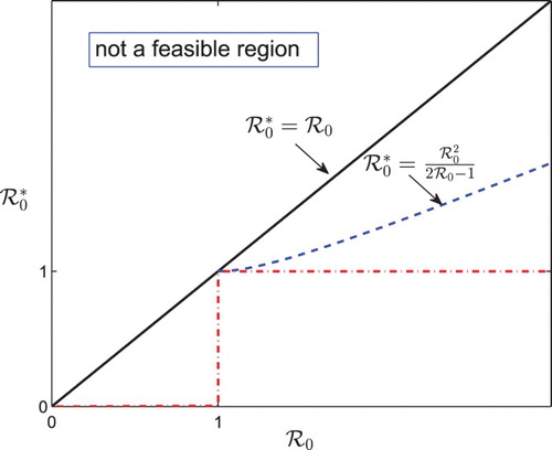
Table 1. Epidemic characteristics of Equation (2(2) $\begin{array}{rl}\frac{\mathrm{d}S}{\mathrm{d}t}& =-\beta S\frac{I}{N},\\ \frac{\mathrm{d}I}{\mathrm{d}t}& =\beta S\frac{I}{N}-\delta I,\\ \frac{\mathrm{d}N}{\mathrm{d}t}& =-\delta I,\end{array}$(2) ) with respect to the reproduction numbers ${\mathcal{R}}_0$ and ${\mathcal{R}}_0^{\ast }$. Note that ${\mathcal{R}}_0^{\ast }$ is always less than ${\mathcal{R}}_0$ based on (12(12) ${\mathcal{R}}_0^{\ast }=\frac{\beta }{\delta }\frac{S_0}{S_0+I_0}=\frac{S_0}{N_0}{\mathcal{R}}_0,$(12) ), also shown in Figure 1.

Basic reproduction	Net reproduction		Outbreak size	Epidemic peak	Turning point
${\mathcal{R}}_0<1$	any ${\mathcal{R}}_0^{\ast }<{\mathcal{R}}_0$		$N_0\left[1-{\left(\frac{{\mathcal{R}}_0}{{\mathcal{R}}_0^{\ast }}\right)}^{1/({\mathcal{R}}_0-1)}\right]$	Not exist	Not exist
${\mathcal{R}}_0\ge 1$	${\mathcal{R}}_0^{\ast }\le 1$		$N_0$
	${\mathcal{R}}_0^{\ast }>1$	${\mathcal{R}}_0^{\ast }\le \frac{{\mathcal{R}}_0^2}{2{\mathcal{R}}_0-1}$		Exists
		${\mathcal{R}}_0^{\ast }>\frac{{\mathcal{R}}_0^2}{2{\mathcal{R}}_0-1}$			Exists

Peak time represents the moment when the infected incidence reaches its maximal value while the turning point quantifies the moment when the growth rate of cumulative cases attains its maximum. Therefore, it is reasonable to expect a time lag from turning point to peak time. Actually, when ${\mathcal{R}}_0^{\ast }>1$, from the expressions of $t_p$ and $t_{\mathrm{T}}$ it follows that $t_{\mathrm{P}}-t_{\mathrm{T}}=\frac{1}{\delta ({\mathcal{R}}_0-1)}\ln {\mathcal{R}}_0>0.$ Hence, the peak time always happens later than the turning point, and the time interval between turning point and peak time is independent of the initial susceptible and infected population sizes $S_0$ and $I_0$ (as well as the net reproduction number ${\mathcal{R}}_0^{\ast }$). Due to the time lag between turning point and peak time, in some surveillance programmes for epidemic outbreaks, one cannot observe the turning point, or both the peak time and turning point.

On the other hand, direct calculation yields the ratio of the infected population sizes at these special moments $\frac{I_{\mathrm{P}}}{I_{\mathrm{T}}}={\mathcal{R}}_0^{-({\mathcal{R}}_0+1)/({\mathcal{R}}_0-1)}(2{\mathcal{R}}_0-1{)}^{{\mathcal{R}}_0/{\mathcal{R}}_0-1},$ implying that the ratio of the peak value of infected cases and the size at the turning point is independent of the net reproduction number (as well as the initial condition). The following lemma shows that $I_{\mathrm{P}}/I_{\mathrm{T}}>1$ for ${\mathcal{R}}_0>1$.

Lemma 3.1.

$x^{-(x+1)/(x-1)}(2x-1{)}^{x/(x-1)}>1\mathrm{forall}x>1.$

Proof.

Denote $g\left(x\right)=x/(x-1)\ln (2x-1)-(x+1)/(x-1)\ln x,$ then $x^{-(x+1)/(x-1)}(2x-1{)}^{x/(x-1)}=e^{g\left(x\right)}$ and it suffices to prove that $g\left(x\right)>0$ for x>1. Direct calculation gives $g^{\prime }\left(x\right)=g_1\left(x\right)/(x-1{)}^2$, with $g_1\left(x\right)=\ln x^2/(2x-1)-(x-1{)}^2/x(2x-1)$. Since $g_1^{\prime }\left(x\right)=(x-1{)}^2(4x-1)/(2x-1{)}^2{x}^2>0$ for x>1, it follows from $g_1\left(1\right)=0$ that $g_1\left(x\right)>0$ for x>1, that is, $g^{\prime }\left(x\right)>0$ for x>1. Further, $\underset{x\to 1+}{lim}g\left(x\right)=0$ implies that $g\left(x\right)>0$ for x>1. The proof is complete.

Finally, it is interesting to highlight the novel conditions for the existence of peak time and turning point in the current paper. If the initial infection size is infinitesimally small relative to the size of susceptibles, the existence of peak time implies the existence of turning point for the number of cumulative cases, and vice versa. Moreover, they exist if and only if the basic reproduction number ${\mathcal{R}}_0$ is greater than unity [12,17]. However, when the initial infection size is not negligible as assumed in the current paper, the existence of peak time (as well as the turning point) is not only dependent on the basic reproduction number ${\mathcal{R}}_0$, but also on the net reproduction number ${\mathcal{R}}_0^{\ast }$. Furthermore, the existence of turning point implies that of the peak time, but not vice versa.

Acknowledgements

The authors are grateful to the anonymous referees for their careful reading and helpful suggestions.

Disclosure statement

No potential conflict of interest was reported by the authors.

Additional information

Funding

The first author is partially supported by NSFC under Grant [11371369]. The second author is partially supported by NSFC under Grant [11301442] and RGC under Grant [PolyU 253004/14P].

References

- F. Brauer, Compartmental models in epidemiology, in Mathematical Epidemiology, Lecture Notes in Mathematics, F. Brauer, P. van den Driessche and J. Wu, eds., Springer, Berlin, 2008, pp. 19–79.
- O. Diekmann, J.A.J. Metz, and J.A.P. Heesterbeek, The legacy of Kermack and McKendrick, in Epidemic Models: Their Structure and Relation to Data, Their Structure and Relation to Data, D. Mollison, ed., Cambridge University Press, Cambridge, 1995, pp. 95–115.
- Z. Feng, Final and peak epidemic sizes for SEIR models with quarantine and isolation, Math. Bios. Eng. 4 (2007), pp. 675–686. doi: 10.3934/mbe.2007.4.675
- Y.H. Hsieh, Richards model: A simple procedure for real-time prediction of outbreak severity, in Modeling and Dynamics of Infectious Diseases, Series in Contemporary Applied Mathematics (CAM), Z.Ma, J.Wu and Y. Zhou, eds., Higher Education Press, Beijing, 2009, pp. 216–236.
- Y. -H. Hsieh, Pandemic influenza A (H1N1) during winter influenza season in the southern hemisphere, Infl. Other Resp. Vir. 4 (2010), pp. 187–197. doi: 10.1111/j.1750-2659.2010.00147.x
- Y. -H. Hsieh and C.W.S. Chen, Turning points, reproduction number, and impact of climatological events for multi-wave dengue outbreaks, Trop. Med. Int. Health 14 (2009), pp. 628–638. doi: 10.1111/j.1365-3156.2009.02277.x
- Y. -H. Hsieh and Y. -S. Cheng, Real-time forecast of multiphase outbreak, Emerg. Infect. Dis. 12 (2006), pp. 122–127. doi: 10.3201/eid1201.050396
- Y. -H. Hsieh, H. dejjArazoza, and R. Lounes, Temporal trends and regional variability of 2001–2002 multiwave DENV-3 epidemic in Havana City: Did Hurricane Michelle contribute to its severity? Trop. Med. Int. Health. 18 (2013), pp. 830–838. doi: 10.1111/tmi.12105
- Y. -H. Hsieh, D.N. Fisman, and J. Wu, On epidemic modeling in real time: An application to the 2009 novel A (H1N1) influenza outbreak in Canada, BMC Res. Notes 3 (2010), p. 283. doi: 10.1186/1756-0500-3-283
- Y. -H. Hsieh, J. -Y. Lee, and H. -L. Chang, SARS epidemiology modeling, Emerg. Infect. Dis. 10 (2004), pp. 1165–1167. doi: 10.3201/eid1006.031023
- Y.H. Hsieh and S. Ma, Intervention measures, turning point, and reproduction number for dengue, Singapore, Am. J. Trop. Med. Hyg. 80 (2005), pp. 66–71.
- Y. -H. Hsieh, J. Wu, J. Fang, Y. Yang, and J. Lou, Quantification of bird-to-bird and bird-to-human infections during 2013 novel H7N9 avian influenza outbreak in China, PLoS ONE 9 (2014), p. e111834. doi: 10.1371/journal.pone.0111834
- J.C. Miller, Epidemics on networks with large initial conditions or changing structure, PLoS ONE 9 (2014), p. e101421. doi: 10.1371/journal.pone.0101421
- F.J. Richards, A flexible growth function for empirical use, J. Exp. Bot. 10 (1959), pp. 290–301. doi: 10.1093/jxb/10.2.290
- J.V. Ross, A note on density-dependence in population models, Ecol. Model. 220 (2009), pp. 3472–3474. doi: 10.1016/j.ecolmodel.2009.08.024
- I. Sazonov, M. Kelbert, and M.B. Gravenor, A two-stage model for the SIR outbreak: Accounting for the discrete and stochastic nature of the epidemic at the initial contamination stage, Math. Biosci. 234 (2011), pp. 108–117. doi: 10.1016/j.mbs.2011.09.002
- X.-S. Wang, J. Wu, and Y. Yang, Richards model revisited: Validation by and application to infection dynamics, J. Theor. Biol. 313 (2012), pp. 12–19. doi: 10.1016/j.jtbi.2012.07.024
- X.-S. Wang and L. Zhong, Ebola outbreak in West Africa: real-time estimation and multiple-wave prediction, Math. Bios. Eng. 12 (2015), pp. 1055–1063. doi: 10.3934/mbe.2015.12.1055
- G. Zhou and G. Yan, Severe acute respiratory syndrome epidemic in Asia, Emerg. Infect. Dis. 9 (2003), pp. 1608–1610.