Modelling and estimation of infectious diseases in a population with heterogeneous dynamic immunity

ABSTRACT

The paper presents a model for the evolution of an infectious disease in a population with individual-specific immunity. The immune state of an individual varies with time according to its own dynamics, depending on whether the individual is infected or not. The model involves a system of size-structured (first-order) PDEs that capture both the dynamics of the immune states and the transition between compartments consisting of infected, susceptible, etc. individuals. Due to the unavailability of precise data about the immune states of the individuals, the main focus in the paper is on developing a technique for set-membership estimations of aggregated quantities of interest. The technique involves solving specific optimization problems for the underlying PDE system and is developed up to a numerical method. Results of numerical simulations are presented for a benchmark model of SIS-type, potentially applicable to diseases like influenza and to various sexually transmitted diseases.

KEYWORDS:

• Mathematical epidemiology
• immunoepidemiology
• immune status
• heterogeneous SIS-models
• size-structured systems
• set-membership estimations

MSC CLASSIFICATION:

• 92D30
• 93E10
• 35F10
• 49K20

1. Introduction

Ever since the seminal work by Kermack and McKendrick [14] compartmental models, such as SIR- or SIS-models, play a prominent role in mathematical epidemiology. The idea behind such models is to divide the population into several groups such as susceptibles (S), infectives (I), and recovered (R), and to study the interactions between these groups and in particular the transition of individuals from one group into another.

It is obvious that the immune system of individuals plays an important role in this process by counteracting the pathogen inside the body. The exact understanding of how this process works and the modelling of in-host dynamics is the aim of immunology. An introduction to this discipline may be found in [20]. In an epidemiological context immunology is important because the state of the immune system influences, for example, the susceptibility, infectivity, and recovery of individuals. The combination of these two disciplines, sometimes referred to as ‘immunoepidemiology’ ([5,11,19]), is therefore a natural consequence. One way to achieve this is to model the within-host dynamics of the pathogen and couple this with an epidemiological model by assuming that the state of within-host dynamics influences the transmission of the pathogen between hosts. This approach has lead to a number of contributions, e.g. [1,3,7,9,10].

We will instead focus on the influence on the epidemiological dynamics of the waning and boosting of the immune response towards a disease. A short explanation of why the immune response increases and decreases depending on exposure to a pathogen can, for example, be found in [5]. One approach to capture the waning of immunity towards a disease is to introduce additional subclasses of, for example, recovered individuals [12,22] or individuals with waning immunity from vaccination [18,21]. This approach has the advantage that the dynamics are still described by an ODE model; however, these ODE systems can become large if many compartments are added. Another approach is to assume that the recovered population is structured with respect to the immune status of the individuals. This approach retains the low-dimensionality of the equations, however at the cost of introducing a PDE into the system [6]. Such systems can also be formulated to include boosting of the immune system for the recovered population as well [5]. Other approaches to model the boosting of the immune system during the infective period leads to models with multiple structured populations [19]. We will study dynamical systems in which every sub-population is structured with respect to the host immunity. An example of such a model can be found in [26].

In this paper we present a model for the evolution of the susceptible and infected subpopulations (SIS-model) in which the immunity of individuals has its own dynamics, depending on whether the individual is susceptible of infected. The model involves a system of first-order PDEs (of the type of the so-called size-structured systems), which is similar to (but different from) [26]. It could be interpreted in terms of an influenza infection, but similar models may be appropriate to simulate sexually transmitted diseases [4]. In [26], it is argued that this framework can also be used to model microparasite infections.

To numerically simulate heterogeneous models, such as the one developed here, the initial distribution of the population along the possible immunity states has to be known. However, precise information about this distribution is not available in practice. Therefore, we develop a method to estimate the dynamics of the disease under uncertain initial conditions, based on available data only. It builds on the general approach of set-membership estimation under deterministic uncertainty (see, e.g. [15–17]).

The paper is organized as follows. In Section 2 we introduce a benchmark SIS-model with heterogeneous immunity, which consists of a pair of size-structured first-order PDEs. In Section 3 we begin the investigation of this model by studying its steady-state distributions. In Section 4 we present a more general class of models (including SIR-models, for example), and develop the appropriate set-membership estimation technique. This allows us to estimate the evolution of the disease without complete knowledge of its initial state. Finally, in Section 5, we apply this technique to the benchmark model to gain additional insights about the steady states found in Section 3 and to study how differences in the initial distribution influence the short- and long-term behaviour of the disease.

2. The heterogeneous SIS model

In the model below we consider a closed population of fixed size, a part of which is infected by influenza. Each individual has an immunity level characterized by a number $\omega \in [0,1]$: the larger is ω, the higher is the immunity of an individual. The level of immunity has its own dynamics. If an individual is susceptible (i.e. not infected, in the present context) in a time interval $[\tau ,\theta )$, then her immunity level obeys the equation (1) $\dot{\omega }\left(t\right)=d\left(\omega \right(t\left)\right),\omega \left(\tau \right)={\omega }_{\tau },t\in [\tau ,\theta ),$(1) where ${\omega }_{\tau }$ is the immunity level at time τ and $d\left(\omega \right)$ is the velocity of decrease of immunity at immune state ω. Thus, $d:[0,1]\to (-\mathrm{\infty },0]$.

Similarly, $e:[0,1]\to [0,\mathrm{\infty })$ represents the velocity of increase of immunity of infected individuals: the dynamics of the immune state of an individual which is infected in $[\theta ,\eta )$ is described by the equation (2) $\dot{\omega }\left(t\right)=e\left(\omega \right(t\left)\right),\omega \left(\theta \right)={\omega }_{\theta },t\in [\theta ,\eta ).$(2) Of course, if a susceptible individual becomes infected at time θ, then the dynamics of her immune level switches from Equation (1(1) $\dot{\omega }\left(t\right)=d\left(\omega \right(t\left)\right),\omega \left(\tau \right)={\omega }_{\tau },t\in [\tau ,\theta ),$(1) ) to (2(2) $\dot{\omega }\left(t\right)=e\left(\omega \right(t\left)\right),\omega \left(\theta \right)={\omega }_{\theta },t\in [\theta ,\eta ).$(2) ), then switches back to Equation (1(1) $\dot{\omega }\left(t\right)=d\left(\omega \right(t\left)\right),\omega \left(\tau \right)={\omega }_{\tau },t\in [\tau ,\theta ),$(1) ) at the time of recovery. In the long run, such switchings may happen several time. Notice that the dynamics of the immune state is not individual-specific – the laws (1(1) $\dot{\omega }\left(t\right)=d\left(\omega \right(t\left)\right),\omega \left(\tau \right)={\omega }_{\tau },t\in [\tau ,\theta ),$(1) ) and (2(2) $\dot{\omega }\left(t\right)=e\left(\omega \right(t\left)\right),\omega \left(\theta \right)={\omega }_{\theta },t\in [\theta ,\eta ).$(2) ) apply to each individual.

In order to ensure existence and uniqueness of the solutions of the above ODEs, and invariance of the interval $[0,1]$ (which is required in order to make the model meaningful) we assume that d and e are continuously differentiable and $d\left(0\right)=e\left(1\right)=0$. This resembles the assumption that the interval $[0,1]$ contains all possible immune states.

Now, we describe the model of the evolution of the susceptible and the infected subpopulations, beginning with some notations. The numbers $S(t,\omega )$ and $I(t,\omega )$ represent the sizes of the susceptible/infected subpopulations of immunity state ω at time t. The susceptibility of a susceptible individual depends on the immunity state and is denoted by $p\left(\omega \right)\ge 0$. The infectivity of an infected individual may also depend on the immunity state and is denoted by $q\left(\omega \right)\ge 0$. The recovery rate of an infected individual of immunity state ω is denoted by $\delta \left(\omega \right)\ge 0$. Finally, $\sigma \left(t\right)\ge 0$ is the strength of infection or effective contact rate. It is reasonably assumed to depend on time in order to capture possible seasonal changes or other time-dependent effects.

Notice that the total population size can be represented as $N\left(t\right)={\int }_0^1\left[S\right(t,\omega )+I(t,\omega \left)\right]\mathrm{d}\omega .$ In the model below, it will be assumed that the total population size remains constant, therefore one may normalize it to $N\left(t\right)=1$. Then under the assumption of proportional mixing (see, e.g. [8]), the incidence rate takes the form (3) $\frac{{\int }_0^{1}q\left(\zeta \right)I(t,\zeta )\mathrm{d}\zeta }{N\left(t\right)}={\int }_0^{1}q\left(\zeta \right)I(t,\zeta )\mathrm{d}\zeta .$(3) The evolution of the susceptible/infected individuals, regarding the changes of the immunity state, is described by the equations (4) $\begin{array}{rl}\frac{\mathrm{\partial }}{\mathrm{\partial }t}S(t,\omega )+\frac{\mathrm{\partial }}{\mathrm{\partial }\omega }\left(d\right(\omega \left)S\right(t,\omega \left)\right)& =-\sigma \left(t\right)p\left(\omega \right){\int }_0^{1}q\left(\zeta \right)I(t,\zeta )\mathrm{d}\zeta S(t,\omega )+\delta \left(\omega \right)I(t,\omega ),\\ \frac{\mathrm{\partial }}{\mathrm{\partial }t}I(t,\omega )+\frac{\mathrm{\partial }}{\mathrm{\partial }\omega }\left(e\right(\omega \left)I\right(t,\omega \left)\right)& =\sigma \left(t\right)p\left(\omega \right){\int }_0^{1}q\left(\zeta \right)I(t,\zeta )\mathrm{d}\zeta S(t,\omega )-\delta \left(\omega \right)I(t,\omega ),\end{array}$(4) complemented with the initial conditions (5) $S(0,\omega )=S^0\left(\omega \right),I(0,\omega )=I^0\left(\omega \right),\omega \in [0,1],$(5) and the boundary (zero-flux) conditions (6) $d\left(1\right)S(t,1)=0,e\left(0\right)I(t,0)=0,t\ge 0.$(6) In our case we will fulfil the zero-flux conditions by assuming that $d\left(1\right)=e\left(0\right)=0$, which is not principally necessary, but is reasonable and makes the analysis technically simpler (see Remark 4.1 in Section 4.1). For simplicity, the data p, q, δ, σ, $S^0$, $I^0$ are assumed to be continuous functions (although this assumption can be easily relaxed – only measurability and boundedness suffice). Also it is reasonably assumed that $d\left(\omega \right)<0$ and $e\left(\omega \right)>0$ for $\omega \in (0,1)$ (strict loss/gain of immunity if not-perfect/missing), and that $p\left(0\right)>0$, $q\left(0\right)>0$. Due to the normalization of the population size, we have to assume also that ${\int }_0^1\left[S^0\right(\omega )+I^0(\omega \left)\right]\mathrm{d}\omega =1$.

Equations (4(4) $\begin{array}{rl}\frac{\mathrm{\partial }}{\mathrm{\partial }t}S(t,\omega )+\frac{\mathrm{\partial }}{\mathrm{\partial }\omega }\left(d\right(\omega \left)S\right(t,\omega \left)\right)& =-\sigma \left(t\right)p\left(\omega \right){\int }_0^{1}q\left(\zeta \right)I(t,\zeta )\mathrm{d}\zeta S(t,\omega )+\delta \left(\omega \right)I(t,\omega ),\\ \frac{\mathrm{\partial }}{\mathrm{\partial }t}I(t,\omega )+\frac{\mathrm{\partial }}{\mathrm{\partial }\omega }\left(e\right(\omega \left)I\right(t,\omega \left)\right)& =\sigma \left(t\right)p\left(\omega \right){\int }_0^{1}q\left(\zeta \right)I(t,\zeta )\mathrm{d}\zeta S(t,\omega )-\delta \left(\omega \right)I(t,\omega ),\end{array}$(4) ) have a clear micro-foundation: they can be derived (like in physics) by calculating what amount of individuals will enter/leave immunity state interval $[\omega ,\omega +\mathrm{\Delta }\omega ]$ in a time horizon $[t,t+\mathrm{\Delta }t]$, and then pass to a limit with $\mathrm{\Delta }t$ and $\mathrm{\Delta }\omega$. This kind of size-structured systems are widely used in mathematical biology, while in the context of epidemiology, we may refer to [19,26].

The exact definition of the notion of solution of equations (4(4) $\begin{array}{rl}\frac{\mathrm{\partial }}{\mathrm{\partial }t}S(t,\omega )+\frac{\mathrm{\partial }}{\mathrm{\partial }\omega }\left(d\right(\omega \left)S\right(t,\omega \left)\right)& =-\sigma \left(t\right)p\left(\omega \right){\int }_0^{1}q\left(\zeta \right)I(t,\zeta )\mathrm{d}\zeta S(t,\omega )+\delta \left(\omega \right)I(t,\omega ),\\ \frac{\mathrm{\partial }}{\mathrm{\partial }t}I(t,\omega )+\frac{\mathrm{\partial }}{\mathrm{\partial }\omega }\left(e\right(\omega \left)I\right(t,\omega \left)\right)& =\sigma \left(t\right)p\left(\omega \right){\int }_0^{1}q\left(\zeta \right)I(t,\zeta )\mathrm{d}\zeta S(t,\omega )-\delta \left(\omega \right)I(t,\omega ),\end{array}$(4) )–(6(6) $d\left(1\right)S(t,1)=0,e\left(0\right)I(t,0)=0,t\ge 0.$(6) ) will be given in Section 4.

Remark 2.1.

In the above model, we assumed in advance (by taking $N\left(t\right)=1$) that the population has constant size. Notice that Equations (4(4) $\begin{array}{rl}\frac{\mathrm{\partial }}{\mathrm{\partial }t}S(t,\omega )+\frac{\mathrm{\partial }}{\mathrm{\partial }\omega }\left(d\right(\omega \left)S\right(t,\omega \left)\right)& =-\sigma \left(t\right)p\left(\omega \right){\int }_0^{1}q\left(\zeta \right)I(t,\zeta )\mathrm{d}\zeta S(t,\omega )+\delta \left(\omega \right)I(t,\omega ),\\ \frac{\mathrm{\partial }}{\mathrm{\partial }t}I(t,\omega )+\frac{\mathrm{\partial }}{\mathrm{\partial }\omega }\left(e\right(\omega \left)I\right(t,\omega \left)\right)& =\sigma \left(t\right)p\left(\omega \right){\int }_0^{1}q\left(\zeta \right)I(t,\zeta )\mathrm{d}\zeta S(t,\omega )-\delta \left(\omega \right)I(t,\omega ),\end{array}$(4) ) together with the zero-flux conditions (6(6) $d\left(1\right)S(t,1)=0,e\left(0\right)I(t,0)=0,t\ge 0.$(6) ) and the natural condition $d\left(0\right)=e\left(1\right)=0$ keep the size of the population constant ($=1$).

Remark 2.2.

The assumption that there is no in/out flow of population is somewhat restrictive. In fact, in- and out-flows of equal amounts of individuals is implicitly included in the model, provided that the flows have the same ω-distributions as the existing population, hence have no effect on S and I. Moreover, the model (4(4) $\begin{array}{rl}\frac{\mathrm{\partial }}{\mathrm{\partial }t}S(t,\omega )+\frac{\mathrm{\partial }}{\mathrm{\partial }\omega }\left(d\right(\omega \left)S\right(t,\omega \left)\right)& =-\sigma \left(t\right)p\left(\omega \right){\int }_0^{1}q\left(\zeta \right)I(t,\zeta )\mathrm{d}\zeta S(t,\omega )+\delta \left(\omega \right)I(t,\omega ),\\ \frac{\mathrm{\partial }}{\mathrm{\partial }t}I(t,\omega )+\frac{\mathrm{\partial }}{\mathrm{\partial }\omega }\left(e\right(\omega \left)I\right(t,\omega \left)\right)& =\sigma \left(t\right)p\left(\omega \right){\int }_0^{1}q\left(\zeta \right)I(t,\zeta )\mathrm{d}\zeta S(t,\omega )-\delta \left(\omega \right)I(t,\omega ),\end{array}$(4) )–(6(6) $d\left(1\right)S(t,1)=0,e\left(0\right)I(t,0)=0,t\ge 0.$(6) ) can be easily enhanced to include out-flows due to mortality (also additional mortality caused by infection) and migration, and in-flows of new-borns and immigrants, having heterogeneous immunity states. This is just a matter of adding new terms in Equations (4(4) $\begin{array}{rl}\frac{\mathrm{\partial }}{\mathrm{\partial }t}S(t,\omega )+\frac{\mathrm{\partial }}{\mathrm{\partial }\omega }\left(d\right(\omega \left)S\right(t,\omega \left)\right)& =-\sigma \left(t\right)p\left(\omega \right){\int }_0^{1}q\left(\zeta \right)I(t,\zeta )\mathrm{d}\zeta S(t,\omega )+\delta \left(\omega \right)I(t,\omega ),\\ \frac{\mathrm{\partial }}{\mathrm{\partial }t}I(t,\omega )+\frac{\mathrm{\partial }}{\mathrm{\partial }\omega }\left(e\right(\omega \left)I\right(t,\omega \left)\right)& =\sigma \left(t\right)p\left(\omega \right){\int }_0^{1}q\left(\zeta \right)I(t,\zeta )\mathrm{d}\zeta S(t,\omega )-\delta \left(\omega \right)I(t,\omega ),\end{array}$(4) ) and replacing the incidence rate with the left term in Equation (3(3) $\frac{{\int }_0^{1}q\left(\zeta \right)I(t,\zeta )\mathrm{d}\zeta }{N\left(t\right)}={\int }_0^{1}q\left(\zeta \right)I(t,\zeta )\mathrm{d}\zeta .$(3) ) in order to take into account a possible change of the population size.

3. Steady states

In this section we investigate the steady states of the benchmark system (4(4) $\begin{array}{rl}\frac{\mathrm{\partial }}{\mathrm{\partial }t}S(t,\omega )+\frac{\mathrm{\partial }}{\mathrm{\partial }\omega }\left(d\right(\omega \left)S\right(t,\omega \left)\right)& =-\sigma \left(t\right)p\left(\omega \right){\int }_0^{1}q\left(\zeta \right)I(t,\zeta )\mathrm{d}\zeta S(t,\omega )+\delta \left(\omega \right)I(t,\omega ),\\ \frac{\mathrm{\partial }}{\mathrm{\partial }t}I(t,\omega )+\frac{\mathrm{\partial }}{\mathrm{\partial }\omega }\left(e\right(\omega \left)I\right(t,\omega \left)\right)& =\sigma \left(t\right)p\left(\omega \right){\int }_0^{1}q\left(\zeta \right)I(t,\zeta )\mathrm{d}\zeta S(t,\omega )-\delta \left(\omega \right)I(t,\omega ),\end{array}$(4) ) in the case of time-invariant strength of infection $\sigma \left(t\right)=\sigma$. Steady states are important in the study of asymptotic behaviour and give valuable information, in general. Although we are, due to the complexity of the model, not able to completely describe the steady states or asymptotic behaviour analytically, the calculations here are the basis for a numerical analysis of the steady states which will be carried out in Section 5.

We formally drop the time dependence of the functions $S(t,\omega )$ and $I(t,\omega )$. This yields (denoting differentiation with respect to ω by ${}^{\prime }$) (7) $\begin{array}{rl}\left(d\right(\omega \left)S\right(\omega ){)}^{\prime }& =-\sigma p\left(\omega \right){\int }_0^{1}q\left(\zeta \right)I\left(\zeta \right)\mathrm{d}\zeta S\left(\omega \right)+\delta \left(\omega \right)I\left(\omega \right),\\ \left(e\right(\omega \left)I\right(\omega ){)}^{\prime }& =\sigma p\left(\omega \right){\int }_0^{1}q\left(\zeta \right)I\left(\zeta \right)\mathrm{d}\zeta S\left(\omega \right)-\delta \left(\omega \right)I\left(\omega \right).\end{array}$(7) Note that we have $\left(d\right(\omega \left)S\right(\omega )+e(\omega \left)I\right(\omega ){)}^{\prime }=0$ which implies (8) $d\left(\omega \right)S\left(\omega \right)+e\left(\omega \right)I\left(\omega \right)=\kappa =\mathrm{const}.$(8) From the zero-flux conditions (6(6) $d\left(1\right)S(t,1)=0,e\left(0\right)I(t,0)=0,t\ge 0.$(6) ) and the assumption $d\left(0\right)=e\left(1\right)=0,$ we obtain that $\kappa =0$.

3.1. Disease free steady states

First, we look for disease free steady states of Equation (7(7) $\begin{array}{rl}\left(d\right(\omega \left)S\right(\omega ){)}^{\prime }& =-\sigma p\left(\omega \right){\int }_0^{1}q\left(\zeta \right)I\left(\zeta \right)\mathrm{d}\zeta S\left(\omega \right)+\delta \left(\omega \right)I\left(\omega \right),\\ \left(e\right(\omega \left)I\right(\omega ){)}^{\prime }& =\sigma p\left(\omega \right){\int }_0^{1}q\left(\zeta \right)I\left(\zeta \right)\mathrm{d}\zeta S\left(\omega \right)-\delta \left(\omega \right)I\left(\omega \right).\end{array}$(7) ), i.e. solutions with $I\left(\omega \right)\equiv 0$. Under this condition (8(8) $d\left(\omega \right)S\left(\omega \right)+e\left(\omega \right)I\left(\omega \right)=\kappa =\mathrm{const}.$(8) ) becomes $d\left(\omega \right)S\left(\omega \right)=0$ which implies $S\left(\omega \right)=0$ for $\omega \in (0,1)$. Since ${\int }_0^{1}S\left(\omega \right)\mathrm{d}\omega =1$, we get that $S\left(\omega \right)=a{\delta }_0\left(\omega \right)+(1-a){\delta }_0(\omega -1)$ for $a\in [0,1]$ and where ${\delta }_0\left(\omega \right)$ is the Dirac-delta. In particular, the only disease free steady state that fulfils the zero-flux condition $d\left(1\right)S\left(1\right)=0$ is $S\left(\omega \right)={\delta }_0\left(\omega \right)$.

3.2. Endemic steady states

Now, we consider the solutions of the steady-state system (7(7) $\begin{array}{rl}\left(d\right(\omega \left)S\right(\omega ){)}^{\prime }& =-\sigma p\left(\omega \right){\int }_0^{1}q\left(\zeta \right)I\left(\zeta \right)\mathrm{d}\zeta S\left(\omega \right)+\delta \left(\omega \right)I\left(\omega \right),\\ \left(e\right(\omega \left)I\right(\omega ){)}^{\prime }& =\sigma p\left(\omega \right){\int }_0^{1}q\left(\zeta \right)I\left(\zeta \right)\mathrm{d}\zeta S\left(\omega \right)-\delta \left(\omega \right)I\left(\omega \right).\end{array}$(7) ), where $I\left(\omega \right)$ is not zero almost everywhere. We furthermore restrict ourselves to solutions where both $S\left(\omega \right)$ and $I\left(\omega \right)$ are non-negative. For this analysis we fix an ${\omega }^{\ast }\in (0,1)$. Furthermore, for $\theta \in (0,\mathrm{\infty })$ we define the three functions (9) $\begin{array}{rl}g\left(\theta \right)& =\frac{\theta }{{\int }_0^{1}q\left(\omega \right){\mathrm{e}}^{-{\int }_{{\omega }^{\ast }}^{\omega }\frac{\sigma p\left(\zeta \right)\theta }{d\left(\zeta \right)}+\frac{\delta \left(\zeta \right)+e^{\prime }\left(\zeta \right)}{e\left(\zeta \right)}\mathrm{d}\zeta }\mathrm{d}\omega },\end{array}$(9) (10) $\begin{array}{rl}{I}_{\theta }\left(\omega \right)& =g\left(\theta \right){\mathrm{e}}^{-{\int }_{{\omega }^{\ast }}^{\omega }\frac{\sigma p\left(\zeta \right)\theta }{d\left(\zeta \right)}+\frac{\delta \left(\zeta \right)+e^{\prime }\left(\zeta \right)}{e\left(\zeta \right)}\mathrm{d}\zeta },\end{array}$(10) (11) $\begin{array}{rl}{S}_{\theta }\left(\omega \right)& =-\frac{e\left(\omega \right)}{d\left(\omega \right)}{I}_{\theta }\left(\omega \right).\end{array}$(11) First, assume that $\left(S^{\ast }\right(\omega ),I^{\ast }(\omega \left)\right)$ solves Equation (7(7) $\begin{array}{rl}\left(d\right(\omega \left)S\right(\omega ){)}^{\prime }& =-\sigma p\left(\omega \right){\int }_0^{1}q\left(\zeta \right)I\left(\zeta \right)\mathrm{d}\zeta S\left(\omega \right)+\delta \left(\omega \right)I\left(\omega \right),\\ \left(e\right(\omega \left)I\right(\omega ){)}^{\prime }& =\sigma p\left(\omega \right){\int }_0^{1}q\left(\zeta \right)I\left(\zeta \right)\mathrm{d}\zeta S\left(\omega \right)-\delta \left(\omega \right)I\left(\omega \right).\end{array}$(7) ) and is non-negative. Define (12) ${\theta }^{\ast }={\int }_0^{1}q\left(\omega \right)I^{\ast }\left(\omega \right)\mathrm{d}\omega .$(12) Using Equations (7(7) $\begin{array}{rl}\left(d\right(\omega \left)S\right(\omega ){)}^{\prime }& =-\sigma p\left(\omega \right){\int }_0^{1}q\left(\zeta \right)I\left(\zeta \right)\mathrm{d}\zeta S\left(\omega \right)+\delta \left(\omega \right)I\left(\omega \right),\\ \left(e\right(\omega \left)I\right(\omega ){)}^{\prime }& =\sigma p\left(\omega \right){\int }_0^{1}q\left(\zeta \right)I\left(\zeta \right)\mathrm{d}\zeta S\left(\omega \right)-\delta \left(\omega \right)I\left(\omega \right).\end{array}$(7) ) and (8(8) $d\left(\omega \right)S\left(\omega \right)+e\left(\omega \right)I\left(\omega \right)=\kappa =\mathrm{const}.$(8) ), it is easy to show for $\omega \in (0,1)$ that $I^{\ast }\left(\omega \right)$ fulfils ${I^{\ast }}^{\prime }\left(\omega \right)=-(\frac{\sigma p\left(\omega \right){\theta }^{\ast }}{d\left(\omega \right)}+\frac{\delta \left(\omega \right)+e^{\prime }\left(\omega \right)}{e\left(\omega \right)})I^{\ast }\left(\omega \right).$ From this we see that for $\omega \in (0,1)$, we can write (13) $I^{\ast }\left(\omega \right)=I^{\ast }\left({\omega }^{\ast }\right){\mathrm{e}}^{-{\int }_{{\omega }^{\ast }}^{\omega }\frac{\sigma p\left(\zeta \right){\theta }^{\ast }}{d\left(\zeta \right)}+\frac{\delta \left(\zeta \right)+e^{\prime }\left(\zeta \right)}{e\left(\zeta \right)}\mathrm{d}\zeta }.$(13) Multiplying this equation by $q\left(\omega \right)$ and integrating over $(0,1)$ yields ${\theta }^{\ast }=I^{\ast }\left({\omega }^{\ast }\right){\int }_0^{1}q\left(\omega \right){\mathrm{e}}^{-{\int }_{{\omega }^{\ast }}^{\omega }\frac{\sigma p\left(\zeta \right){\theta }^{\ast }}{d\left(\zeta \right)}+\frac{\delta \left(\zeta \right)+e^{\prime }\left(\zeta \right)}{e\left(\zeta \right)}\mathrm{d}\zeta }\mathrm{d}\omega ,$ which is equivalent to $I^{\ast }\left({\omega }^{\ast }\right)=g\left({\theta }^{\ast }\right)$. Plugging this into Equation (13(11) $\begin{array}{rl}{S}_{\theta }\left(\omega \right)& =-\frac{e\left(\omega \right)}{d\left(\omega \right)}{I}_{\theta }\left(\omega \right).\end{array}$(11) ), we see that $I^{\ast }\left(\omega \right)=I_{{\theta }^{\ast }}\left(\omega \right)$, and using Equation (8(8) $d\left(\omega \right)S\left(\omega \right)+e\left(\omega \right)I\left(\omega \right)=\kappa =\mathrm{const}.$(8) ), that $S^{\ast }\left(\omega \right)=S_{{\theta }^{\ast }}\left(\omega \right)$. Note that because the solution is assumed to be non-negative and that $I^{\ast }\left(\omega \right)$ is not identically zero, we get that ${\theta }^{\ast }>0$.

Now conversely assume that $\theta >0$. Then it is obvious that $I_{\theta }$ and $S_{\theta }$ are both non-negative, as $g\left(\theta \right)>0$. Due to our definition of $g\left(\theta \right)$, it is easy to see that ${\int }_0^{1}q\left(\omega \right)I_{\theta }\left(\omega \right)\mathrm{d}\omega =\theta$. Using this, by a simple differentiation of Equation (10(10) $\begin{array}{rl}{I}_{\theta }\left(\omega \right)& =g\left(\theta \right){\mathrm{e}}^{-{\int }_{{\omega }^{\ast }}^{\omega }\frac{\sigma p\left(\zeta \right)\theta }{d\left(\zeta \right)}+\frac{\delta \left(\zeta \right)+e^{\prime }\left(\zeta \right)}{e\left(\zeta \right)}\mathrm{d}\zeta },\end{array}$(10) ), we obtain that for $\omega \in (0,1)$ (14) $I_{\theta }^{\prime }\left(\omega \right)=-\frac{\sigma p\left(\omega \right){\int }_0^{1}q\left(\zeta \right)I_{\theta }\left(\zeta \right)\mathrm{d}\zeta }{d\left(\omega \right)}{I}_{\theta }\left(\omega \right)-\frac{\delta \left(\omega \right)+e^{\prime }\left(\omega \right)}{e\left(\omega \right)}{I}_{\theta }\left(\omega \right).$(14) Multiplying Equation (11(11) $\begin{array}{rl}{S}_{\theta }\left(\omega \right)& =-\frac{e\left(\omega \right)}{d\left(\omega \right)}{I}_{\theta }\left(\omega \right).\end{array}$(11) ) with $d\left(\omega \right)/e\left(\omega \right)$ and plugging the result into Equation (14(12) ${\theta }^{\ast }={\int }_0^{1}q\left(\omega \right)I^{\ast }\left(\omega \right)\mathrm{d}\omega .$(12) ), then multiplying by $e\left(\omega \right)$ yields $\left(e\right(\omega \left)I_{\theta }\right(\omega ){)}^{\prime }=\sigma p(\omega \left){\int }_0^{1}q\right(\zeta \left)I_{\theta }\right(\zeta \left)\mathrm{d}\zeta S_{\theta }\right(\omega )-\delta (\omega \left)I_{\theta }\right(\omega ).$ Consequently, $\left(S_{\theta }\right(\omega ),I_{\theta }(\omega \left)\right)$ solves Equation (7(7) $\begin{array}{rl}\left(d\right(\omega \left)S\right(\omega ){)}^{\prime }& =-\sigma p\left(\omega \right){\int }_0^{1}q\left(\zeta \right)I\left(\zeta \right)\mathrm{d}\zeta S\left(\omega \right)+\delta \left(\omega \right)I\left(\omega \right),\\ \left(e\right(\omega \left)I\right(\omega ){)}^{\prime }& =\sigma p\left(\omega \right){\int }_0^{1}q\left(\zeta \right)I\left(\zeta \right)\mathrm{d}\zeta S\left(\omega \right)-\delta \left(\omega \right)I\left(\omega \right).\end{array}$(7) ) on the open interval $(0,1)$. Thus, we have proven the following theorem.

Theorem 3.1.

Choose ${\omega }^{\ast }\in (0,1)$. Let $g\left(\theta \right),$ $I_{\theta }\left(\omega \right)$ and $S_{\theta }\left(\omega \right)$ be defined as in Equations (9(9) $\begin{array}{rl}g\left(\theta \right)& =\frac{\theta }{{\int }_0^{1}q\left(\omega \right){\mathrm{e}}^{-{\int }_{{\omega }^{\ast }}^{\omega }\frac{\sigma p\left(\zeta \right)\theta }{d\left(\zeta \right)}+\frac{\delta \left(\zeta \right)+e^{\prime }\left(\zeta \right)}{e\left(\zeta \right)}\mathrm{d}\zeta }\mathrm{d}\omega },\end{array}$(9) )–(11(11) $\begin{array}{rl}{S}_{\theta }\left(\omega \right)& =-\frac{e\left(\omega \right)}{d\left(\omega \right)}{I}_{\theta }\left(\omega \right).\end{array}$(11) ) respectively.

• If $\theta >0,$ then $\left(S_{\theta }\right(\omega ),I_{\theta }(\omega \left)\right)$ solves Equation (7(7) $\begin{array}{rl}\left(d\right(\omega \left)S\right(\omega ){)}^{\prime }& =-\sigma p\left(\omega \right){\int }_0^{1}q\left(\zeta \right)I\left(\zeta \right)\mathrm{d}\zeta S\left(\omega \right)+\delta \left(\omega \right)I\left(\omega \right),\\ \left(e\right(\omega \left)I\right(\omega ){)}^{\prime }& =\sigma p\left(\omega \right){\int }_0^{1}q\left(\zeta \right)I\left(\zeta \right)\mathrm{d}\zeta S\left(\omega \right)-\delta \left(\omega \right)I\left(\omega \right).\end{array}$(7) ) for all $\omega \in (0,1)$.

• If $\left(S^{\ast }\right(\omega ),I^{\ast }(\omega \left)\right)$ solves Equation (7(7) $\begin{array}{rl}\left(d\right(\omega \left)S\right(\omega ){)}^{\prime }& =-\sigma p\left(\omega \right){\int }_0^{1}q\left(\zeta \right)I\left(\zeta \right)\mathrm{d}\zeta S\left(\omega \right)+\delta \left(\omega \right)I\left(\omega \right),\\ \left(e\right(\omega \left)I\right(\omega ){)}^{\prime }& =\sigma p\left(\omega \right){\int }_0^{1}q\left(\zeta \right)I\left(\zeta \right)\mathrm{d}\zeta S\left(\omega \right)-\delta \left(\omega \right)I\left(\omega \right).\end{array}$(7) ), define ${\theta }^{\ast }$ as in Equation (12(10) $\begin{array}{rl}{I}_{\theta }\left(\omega \right)& =g\left(\theta \right){\mathrm{e}}^{-{\int }_{{\omega }^{\ast }}^{\omega }\frac{\sigma p\left(\zeta \right)\theta }{d\left(\zeta \right)}+\frac{\delta \left(\zeta \right)+e^{\prime }\left(\zeta \right)}{e\left(\zeta \right)}\mathrm{d}\zeta },\end{array}$(10) ). Then ${\theta }^{\ast }>0$ and $\left(S^{\ast }\right(\omega ),I^{\ast }(\omega \left)\right)=\left(S_{{\theta }^{\ast }}\right(\omega ),I_{{\theta }^{\ast }}(\omega \left)\right)$ for all $\omega \in (0,1)$.

This theorem shows that there is a one-to-one correspondence between non-negative solutions of Equation (7(7) $\begin{array}{rl}\left(d\right(\omega \left)S\right(\omega ){)}^{\prime }& =-\sigma p\left(\omega \right){\int }_0^{1}q\left(\zeta \right)I\left(\zeta \right)\mathrm{d}\zeta S\left(\omega \right)+\delta \left(\omega \right)I\left(\omega \right),\\ \left(e\right(\omega \left)I\right(\omega ){)}^{\prime }& =\sigma p\left(\omega \right){\int }_0^{1}q\left(\zeta \right)I\left(\zeta \right)\mathrm{d}\zeta S\left(\omega \right)-\delta \left(\omega \right)I\left(\omega \right).\end{array}$(7) ) on $(0,1)$ and positive numbers θ. In general, the total population N in these solutions is not 1, as is assumed in our case. We are therefore now looking for solutions for which this condition is fulfilled. Using Equations (10(10) $\begin{array}{rl}{I}_{\theta }\left(\omega \right)& =g\left(\theta \right){\mathrm{e}}^{-{\int }_{{\omega }^{\ast }}^{\omega }\frac{\sigma p\left(\zeta \right)\theta }{d\left(\zeta \right)}+\frac{\delta \left(\zeta \right)+e^{\prime }\left(\zeta \right)}{e\left(\zeta \right)}\mathrm{d}\zeta },\end{array}$(10) ) and (11(11) $\begin{array}{rl}{S}_{\theta }\left(\omega \right)& =-\frac{e\left(\omega \right)}{d\left(\omega \right)}{I}_{\theta }\left(\omega \right).\end{array}$(11) ) this yields $\begin{array}{rl}1& ={\int }_0^1{I}_{\theta }\left(\omega \right)+S_{\theta }\left(\omega \right)\mathrm{d}\omega \\ & ={\int }_0^{1}g\left(\theta \right){\mathrm{e}}^{-{\int }_{{\omega }^{\ast }}^{\omega }\frac{\sigma p\left(\zeta \right)\theta }{d\left(\zeta \right)}+\frac{\delta \left(\zeta \right)+e^{\prime }\left(\zeta \right)}{e\left(\zeta \right)}\mathrm{d}\zeta }-\frac{e\left(\omega \right)}{d\left(\omega \right)}g\left(\theta \right){\mathrm{e}}^{-{\int }_{{\omega }^{\ast }}^{\omega }\frac{\sigma p\left(\zeta \right)\theta }{d\left(\zeta \right)}+\frac{\delta \left(\zeta \right)+e^{\prime }\left(\zeta \right)}{e\left(\zeta \right)}\mathrm{d}\zeta }\mathrm{d}\omega \\ & =g\left(\theta \right){\int }_0^1(1-\frac{e\left(\omega \right)}{d\left(\omega \right)}){\mathrm{e}}^{-{\int }_{{\omega }^{\ast }}^{\omega }\frac{\sigma p\left(\zeta \right)\theta }{d\left(\zeta \right)}+\frac{\delta \left(\zeta \right)+e^{\prime }\left(\zeta \right)}{e\left(\zeta \right)}\mathrm{d}\zeta }\mathrm{d}\omega .\end{array}$ Using Equation (9(9) $\begin{array}{rl}g\left(\theta \right)& =\frac{\theta }{{\int }_0^{1}q\left(\omega \right){\mathrm{e}}^{-{\int }_{{\omega }^{\ast }}^{\omega }\frac{\sigma p\left(\zeta \right)\theta }{d\left(\zeta \right)}+\frac{\delta \left(\zeta \right)+e^{\prime }\left(\zeta \right)}{e\left(\zeta \right)}\mathrm{d}\zeta }\mathrm{d}\omega },\end{array}$(9) ), we see that for $\theta \in (0,\mathrm{\infty })$ this is equivalent to $r\left(\theta \right)=0,$ where $r\left(\theta \right)$ is defined as (15) $r\left(\theta \right)={\int }_0^1((1-\frac{e\left(\omega \right)}{d\left(\omega \right)})\theta -q(\omega \left)\right){\mathrm{e}}^{-{\int }_{{\omega }^{\ast }}^{\omega }\frac{\sigma p\left(\zeta \right)\theta }{d\left(\zeta \right)}+\frac{\delta \left(\zeta \right)+e^{\prime }\left(\zeta \right)}{e\left(\zeta \right)}\mathrm{d}\zeta }\mathrm{d}\omega .$(15) We see that $r\left(0\right)<0$ (possibly $-\mathrm{\infty }$) and $r\left(\theta \right)>0$ (again possibly infinite) for any θ bigger than $\underset{\omega \in [0,1]}{sup}q\left(\omega \right)=:Q$. Therefore any solution of the equation $r\left(\theta \right)=0$ must lie in the interval $(0,Q)$. With this notation, we arrive at the following corollary.

Corollary 3.1.

The system (7(7) $\begin{array}{rl}\left(d\right(\omega \left)S\right(\omega ){)}^{\prime }& =-\sigma p\left(\omega \right){\int }_0^{1}q\left(\zeta \right)I\left(\zeta \right)\mathrm{d}\zeta S\left(\omega \right)+\delta \left(\omega \right)I\left(\omega \right),\\ \left(e\right(\omega \left)I\right(\omega ){)}^{\prime }& =\sigma p\left(\omega \right){\int }_0^{1}q\left(\zeta \right)I\left(\zeta \right)\mathrm{d}\zeta S\left(\omega \right)-\delta \left(\omega \right)I\left(\omega \right).\end{array}$(7) ) has a solution that fulfils the zero-flux condition, is non-negative, and fulfils N=1 if and only if the function $r\left(\theta \right)$ has a root ${\theta }^{\ast }\in (0,Q)$. In this case, the solution is given by $(S_{{\theta }^{\ast }},I_{{\theta }^{\ast }})$. This solution is unique if and only if this root is unique.

We note that one can show that $r\left(\theta \right)$ is continuous on the set where it is bounded. The question of the existence of a solution to $r\left(\theta \right)=0$ is therefore closely connected to the question of where $r\left(\theta \right)$ is bounded. This however, cannot be answered in general and depends on the particular choice of parameter functions. The same applies to the uniqueness.

In epidemiological models, it is common that one can define an indicator λ such that if λ is below a certain threshold there exists no endemic steady state, and there exists a unique steady state if λ is above this threshold. In the current context, such an indicator could be the number of roots of $r\left(\theta \right)$ in $[0,Q]$. It is an open question to obtain an indicator of similar kind as the basic reproduction number.

4. Set-membership estimation

In order to calculate a solution of system (4(4) $\begin{array}{rl}\frac{\mathrm{\partial }}{\mathrm{\partial }t}S(t,\omega )+\frac{\mathrm{\partial }}{\mathrm{\partial }\omega }\left(d\right(\omega \left)S\right(t,\omega \left)\right)& =-\sigma \left(t\right)p\left(\omega \right){\int }_0^{1}q\left(\zeta \right)I(t,\zeta )\mathrm{d}\zeta S(t,\omega )+\delta \left(\omega \right)I(t,\omega ),\\ \frac{\mathrm{\partial }}{\mathrm{\partial }t}I(t,\omega )+\frac{\mathrm{\partial }}{\mathrm{\partial }\omega }\left(e\right(\omega \left)I\right(t,\omega \left)\right)& =\sigma \left(t\right)p\left(\omega \right){\int }_0^{1}q\left(\zeta \right)I(t,\zeta )\mathrm{d}\zeta S(t,\omega )-\delta \left(\omega \right)I(t,\omega ),\end{array}$(4) ), one needs to know the initial distributions of the susceptible and infected subpopulations along the heterogeneity ω, that is, $S(0,\omega )$ and $I(0,\omega )$. However, this information is usually not available in detail. We may assume that the total number of susceptible and infected individuals at time 0, that is, the quantities $S\left(0\right)={\int }_0^{1}S(0,\omega )\mathrm{d}\omega$ and $I\left(0\right)={\int }_0^{1}I(0,\omega )\mathrm{d}\omega$, are known. We may also have additional information about the initial distributions, for example, point-wise constraints of the form $u\left(\omega \right):=\left(S\right(0,\omega ),I(0,\omega \left)\right)\in \left[{\phi }_1\right(\omega ),{\phi }_2(\omega \left)\right]$ where ${\phi }_1$ and ${\phi }_2$ are known functions. More generally, we summarize the available information about the initial data as $u(\cdot )\in \mathcal{U}$, where $\mathcal{U}$ is a closed, convex and bounded subset of $L_{\mathrm{\infty }}:=L_{\mathrm{\infty }}\left(\right[0,1]\mapsto {\mathbb{R}}_{+}^n)$. Below in this section, we will formulate the problem of set-membership estimation of the aggregated state of the system, $y\left(t\right):=\left({\int }_0^{1}S\right(t,\omega )\mathrm{d}\omega ,{\int }_0^{1}I(t,\omega \left)\mathrm{d}\omega \right)$, based on the information $u(\cdot )\in \mathcal{U}$ about the initial data and the systems dynamics. Moreover, a computational tool for finding (approximating) the set-membership estimation will be provided. This will be done in a more general framework, including other (also higher dimensional) models of interest in epidemiology and beyond.

4.1. Formulation of the general model

Below $x:[0,T]\times [0,1]\to {\mathbb{R}}^n$ will be viewed as a distributed state function and $y:[0,T]\to {\mathbb{R}}^m$ – as an aggregated state function, with their dynamics given by the equations (16) $\begin{array}{rl}\frac{\mathrm{\partial }}{\mathrm{\partial }t}x(t,\omega )+\frac{\mathrm{\partial }}{\mathrm{\partial }\omega }\left(A\right(\omega \left)x\right(t,\omega \left)\right)& =f(t,\omega ,x(t,\omega ),y(t\left)\right),x(0,\omega )=u\left(\omega \right),\end{array}$(16) (17) $\begin{array}{rl}y\left(t\right)& ={\int }_0^{1}g(t,\omega ,x(t,\omega \left)\right)\mathrm{d}\omega .\end{array}$(17)

The following assumptions will be standing in this section. The function $f:[0,T]\times [0,1]\times {\mathbb{R}}^n\times {\mathbb{R}}^m\to {\mathbb{R}}^n$ is differentiable in x and y, the derivatives $f_x$ and $f_y$ and f itself are measurable in $(t,\omega )$, locally essentially bounded, and locally Lipschitz continuous in $(x,y)$ uniformly in $(t,\omega )$. The function $g:[0,T]\times [0,1]\times {\mathbb{R}}^n\to {\mathbb{R}}^m$ is differentiable in x, the derivative $g_x$ and the function g itself are measurable in ω and continuous in t, locally essentially bounded, and locally Lipschitz continuous in x uniformly in $(t,\omega )$. Moreover, $f(t,\omega ,x,y)\ge -cx$, $g(t,\omega ,x)\ge 0$, where $c\ge 0$ is a constant and the inequalities (understood component-wise) hold for every $(t,\omega )$ and every $x\ge 0$ and $y\ge 0$. The matrix function $A:[0,1]\to {\mathbb{R}}^n\times {\mathbb{R}}^n$ is diagonal with continuously differentiable diagonal elements $a_i\left(\omega \right)$, $a_i\left(0\right)=a_i\left(1\right)=0$ and $a_i\left(\omega \right)\ne 0$ for $\omega \in (0,1)$.

Remark 4.1.

The assumptions about f and g are fulfilled in our model (4(4) $\begin{array}{rl}\frac{\mathrm{\partial }}{\mathrm{\partial }t}S(t,\omega )+\frac{\mathrm{\partial }}{\mathrm{\partial }\omega }\left(d\right(\omega \left)S\right(t,\omega \left)\right)& =-\sigma \left(t\right)p\left(\omega \right){\int }_0^{1}q\left(\zeta \right)I(t,\zeta )\mathrm{d}\zeta S(t,\omega )+\delta \left(\omega \right)I(t,\omega ),\\ \frac{\mathrm{\partial }}{\mathrm{\partial }t}I(t,\omega )+\frac{\mathrm{\partial }}{\mathrm{\partial }\omega }\left(e\right(\omega \left)I\right(t,\omega \left)\right)& =\sigma \left(t\right)p\left(\omega \right){\int }_0^{1}q\left(\zeta \right)I(t,\zeta )\mathrm{d}\zeta S(t,\omega )-\delta \left(\omega \right)I(t,\omega ),\end{array}$(4) ) with $x=(S,I)$ and $y\left(t\right)$ as in the beginning of the present section. Moreover, there we have $A=\mathrm{diag}(d,e)$ and the assumptions about A are fulfilled if d and e are as assumed in Section 2. We stress that the additional assumption $d\left(1\right)=e\left(0\right)=0$ made there provides one way to satisfy the zero-flux conditions (6(6) $d\left(1\right)S(t,1)=0,e\left(0\right)I(t,0)=0,t\ge 0.$(6) ). In this case, Equations (16(14) $I_{\theta }^{\prime }\left(\omega \right)=-\frac{\sigma p\left(\omega \right){\int }_0^{1}q\left(\zeta \right)I_{\theta }\left(\zeta \right)\mathrm{d}\zeta }{d\left(\omega \right)}{I}_{\theta }\left(\omega \right)-\frac{\delta \left(\omega \right)+e^{\prime }\left(\omega \right)}{e\left(\omega \right)}{I}_{\theta }\left(\omega \right).$(14) ), (17(17) $\begin{array}{rl}y\left(t\right)& ={\int }_0^{1}g(t,\omega ,x(t,\omega \left)\right)\mathrm{d}\omega .\end{array}$(17) ) require only initial conditions to produce a unique solution (see below). If $d\left(1\right)\ne 0$ and/or $e\left(0\right)\ne 0$, then the zero-flux conditions must be ensured by adding the boundary conditions $S(t,1)=0$ and/or $I(t,0)=0$ (see, e.g. the more general consideration in [2]). The approach below is still applicable, but the calculations become more cumbersome.

As it will be seen below, a solution of Equations (16(14) $I_{\theta }^{\prime }\left(\omega \right)=-\frac{\sigma p\left(\omega \right){\int }_0^{1}q\left(\zeta \right)I_{\theta }\left(\zeta \right)\mathrm{d}\zeta }{d\left(\omega \right)}{I}_{\theta }\left(\omega \right)-\frac{\delta \left(\omega \right)+e^{\prime }\left(\omega \right)}{e\left(\omega \right)}{I}_{\theta }\left(\omega \right).$(14) ) and (17(17) $\begin{array}{rl}y\left(t\right)& ={\int }_0^{1}g(t,\omega ,x(t,\omega \left)\right)\mathrm{d}\omega .\end{array}$(17) ) is uniquely defined by the initial condition (18) $x(0,\omega )=u\left(\omega \right),\omega \in [0,1],$(18) where $u:[0,1]\mapsto {\mathbb{R}}_{+}^n$ is a measurable and bounded function.

The notion of solution of system (16(14) $I_{\theta }^{\prime }\left(\omega \right)=-\frac{\sigma p\left(\omega \right){\int }_0^{1}q\left(\zeta \right)I_{\theta }\left(\zeta \right)\mathrm{d}\zeta }{d\left(\omega \right)}{I}_{\theta }\left(\omega \right)-\frac{\delta \left(\omega \right)+e^{\prime }\left(\omega \right)}{e\left(\omega \right)}{I}_{\theta }\left(\omega \right).$(14) )–(18(15) $r\left(\theta \right)={\int }_0^1((1-\frac{e\left(\omega \right)}{d\left(\omega \right)})\theta -q(\omega \left)\right){\mathrm{e}}^{-{\int }_{{\omega }^{\ast }}^{\omega }\frac{\sigma p\left(\zeta \right)\theta }{d\left(\zeta \right)}+\frac{\delta \left(\zeta \right)+e^{\prime }\left(\zeta \right)}{e\left(\zeta \right)}\mathrm{d}\zeta }\mathrm{d}\omega .$(15) ) can be defined in several ways, but for the considered problem the method of characteristics seem to be most natural. Let for $i=1,\dots ,n$, the function ${\omega }_i:[0,T]\times [0,1]\to [0,1]$ be defined as the unique solution of the initial value problem $\frac{\mathrm{\partial }}{\mathrm{\partial }t}{\omega }_i(t,\rho )=a_i\left({\omega }_i\right(t,\rho \left)\right),{\omega }_i(0,\rho )=\rho ,$ where ρ is regarded as a parameter for ${\omega }_i$. Due to the assumptions about $a_i\left(\omega \right)$, the mapping $(t,\rho )\mapsto (t,{\omega }_i((t,\rho ))$ is a diffeomorphism of $[0,T]\times [0,1]$ onto itself. Its inverse has the form $(t,\omega )\mapsto (t,{\rho }_i(t,\omega \left)\right)$, where ${\rho }_i$ is continuously differentiable and satisfies ${\omega }_i(t,{\rho }_i(t,\omega \left)\right)=\omega$ and ${\rho }_i(t,{\omega }_i(t,\rho \left)\right)=\rho$.

As a motivation for the definition below, we assume that x is a continuously differentiable solution of Equations (16(14) $I_{\theta }^{\prime }\left(\omega \right)=-\frac{\sigma p\left(\omega \right){\int }_0^{1}q\left(\zeta \right)I_{\theta }\left(\zeta \right)\mathrm{d}\zeta }{d\left(\omega \right)}{I}_{\theta }\left(\omega \right)-\frac{\delta \left(\omega \right)+e^{\prime }\left(\omega \right)}{e\left(\omega \right)}{I}_{\theta }\left(\omega \right).$(14) )–(18(15) $r\left(\theta \right)={\int }_0^1((1-\frac{e\left(\omega \right)}{d\left(\omega \right)})\theta -q(\omega \left)\right){\mathrm{e}}^{-{\int }_{{\omega }^{\ast }}^{\omega }\frac{\sigma p\left(\zeta \right)\theta }{d\left(\zeta \right)}+\frac{\delta \left(\zeta \right)+e^{\prime }\left(\zeta \right)}{e\left(\zeta \right)}\mathrm{d}\zeta }\mathrm{d}\omega .$(15) ). Denote $z_i(t,\rho )=x_i(t,{\omega }_i(t,\rho \left)\right)$, thus $x_i(t,\omega )=z_i(t,{\rho }_i(t,\omega \left)\right)$. Then $\begin{array}{rl}\frac{\mathrm{d}}{\mathrm{d}t}{z}_i(t,\rho )& =\frac{\mathrm{\partial }}{\mathrm{\partial }t}{x}_i(t,{\omega }_i(t,\rho \left)\right)+a_i\left({\omega }_i\right(t,\rho \left)\right)\frac{\mathrm{\partial }}{\mathrm{\partial }\omega }{x}_i(t,{\omega }_i(t,\rho \left)\right),\\ z_i(0,\rho )& =x_i(0,{\omega }_i(0,\rho \left)\right)=x_i(0,\rho )=u\left(\rho \right),\end{array}$ hence (19) $\begin{array}{rl}\frac{\mathrm{d}}{\mathrm{d}t}{z}_i(t,\rho )& =f_i(t,{\omega }_i(t,\rho ),x(t,{\omega }_i(t,\rho )),y(t\left)\right)-a_i^{\prime }\left({\omega }_i\right(t,\rho \left)\right)z_i(t,\rho ),\end{array}$(19) (20) $\begin{array}{rl}{z}_i(0,\rho )& =u\left(\rho \right).\end{array}$(20)

The above equations motivate the following definition (cf. [2]).

Definition 4.1.

The pair of functions $x:[0,T]\times [0,1]\to {\mathbb{R}}^n$ and $y[0,T]\to {\mathbb{R}}^m$ is a solution of system (16(14) $I_{\theta }^{\prime }\left(\omega \right)=-\frac{\sigma p\left(\omega \right){\int }_0^{1}q\left(\zeta \right)I_{\theta }\left(\zeta \right)\mathrm{d}\zeta }{d\left(\omega \right)}{I}_{\theta }\left(\omega \right)-\frac{\delta \left(\omega \right)+e^{\prime }\left(\omega \right)}{e\left(\omega \right)}{I}_{\theta }\left(\omega \right).$(14) )–(18(15) $r\left(\theta \right)={\int }_0^1((1-\frac{e\left(\omega \right)}{d\left(\omega \right)})\theta -q(\omega \left)\right){\mathrm{e}}^{-{\int }_{{\omega }^{\ast }}^{\omega }\frac{\sigma p\left(\zeta \right)\theta }{d\left(\zeta \right)}+\frac{\delta \left(\zeta \right)+e^{\prime }\left(\zeta \right)}{e\left(\zeta \right)}\mathrm{d}\zeta }\mathrm{d}\omega .$(15) ) if x has the representation $x_i(t,{\omega }_i(t,\rho \left)\right)=z_i(t,\rho )$, $t\in [0,T]$, $\rho \in [0,1]$, where $z_i(t,\rho )$ is measurable in ρ and absolutely continuous in t for a.e. ρ, and Equations (19(16) $\begin{array}{rl}\frac{\mathrm{\partial }}{\mathrm{\partial }t}x(t,\omega )+\frac{\mathrm{\partial }}{\mathrm{\partial }\omega }\left(A\right(\omega \left)x\right(t,\omega \left)\right)& =f(t,\omega ,x(t,\omega ),y(t\left)\right),x(0,\omega )=u\left(\omega \right),\end{array}$(16) ), (20(20) $\begin{array}{rl}{z}_i(0,\rho )& =u\left(\rho \right).\end{array}$(20) ) and (17(17) $\begin{array}{rl}y\left(t\right)& ={\int }_0^{1}g(t,\omega ,x(t,\omega \left)\right)\mathrm{d}\omega .\end{array}$(17) ) are satisfied almost everywhere.

The definition is correct and x is a measurable function due to the measurability of z and the fact that $(t,\rho )\mapsto (t,{\omega }_i((t,\rho ))$ is a diffeomorphism. For the same reason, the functions $x_j(t,{\omega }_i(t,\rho \left)\right)=z_j(t,{\rho }_j(t,{\omega }_i(t,\rho )\left)\right)$ in the right-hand side of Equation (19(16) $\begin{array}{rl}\frac{\mathrm{\partial }}{\mathrm{\partial }t}x(t,\omega )+\frac{\mathrm{\partial }}{\mathrm{\partial }\omega }\left(A\right(\omega \left)x\right(t,\omega \left)\right)& =f(t,\omega ,x(t,\omega ),y(t\left)\right),x(0,\omega )=u\left(\omega \right),\end{array}$(16) ) are well-defined and measurable. A solution x does not need to be differentiable. It may even be discontinuous in each of the directions t and ω, but $x_i$ is absolutely continuous along almost every characteristic line $(t,{\omega }_i(t\left)\right)$.

Lemma 4.1.

If $(x,y)$ is a solution of Equations (16(14) $I_{\theta }^{\prime }\left(\omega \right)=-\frac{\sigma p\left(\omega \right){\int }_0^{1}q\left(\zeta \right)I_{\theta }\left(\zeta \right)\mathrm{d}\zeta }{d\left(\omega \right)}{I}_{\theta }\left(\omega \right)-\frac{\delta \left(\omega \right)+e^{\prime }\left(\omega \right)}{e\left(\omega \right)}{I}_{\theta }\left(\omega \right).$(14) )–(18(15) $r\left(\theta \right)={\int }_0^1((1-\frac{e\left(\omega \right)}{d\left(\omega \right)})\theta -q(\omega \left)\right){\mathrm{e}}^{-{\int }_{{\omega }^{\ast }}^{\omega }\frac{\sigma p\left(\zeta \right)\theta }{d\left(\zeta \right)}+\frac{\delta \left(\zeta \right)+e^{\prime }\left(\zeta \right)}{e\left(\zeta \right)}\mathrm{d}\zeta }\mathrm{d}\omega .$(15) ) then the mappings $[0,T]\ni t\mapsto x(t,\cdot )\in L_1(0,1)\text{and}[0,T]\ni t\mapsto y\left(t\right)$ are continuous.

Proof.

The second claim follows from the first due to the Lipschitz continuity of g in x and the boundedness of x. Let us prove the first claim. For every $i=1,\dots ,n$ and for a.e. $t,\tau \in [0,1]$, we have by change of the variable $\omega ={\omega }_i(t,\rho )$ $\begin{array}{rl}& {\int }_0^1|x_i(t,\omega )-x_i(\tau ,\omega )|\mathrm{d}\omega \\ & ={\int }_0^1|x_i(t,{\omega }_i(t,\rho \left)\right)-x_i(\tau ,{\omega }_i(t,\rho \left)\right)|\frac{\mathrm{\partial }}{\mathrm{\partial }\rho }{\omega }_i(t,\rho )\mathrm{d}\rho \\ & \le {\int }_0^1\left[|x_i\right(t,{\omega }_i(t,\rho ))-x_i(\tau ,{\omega }_i(\tau ,\rho ))|+|x_i(\tau ,{\omega }_i(t,\rho ))-x_i(\tau ,{\omega }_i(\tau ,\rho )\left)|\right]\\ & \times \frac{\mathrm{\partial }}{\mathrm{\partial }\rho }{\omega }_i(t,\rho )\mathrm{d}\rho \\ & ={\int }_0^1|z_i(t,\rho )-z_i(\tau ,\rho )|\frac{\mathrm{\partial }}{\mathrm{\partial }\rho }{\omega }_i(t,\rho )\mathrm{d}\rho +{\int }_0^1|x_i(\tau ,\omega )-x_i(\tau ,{\omega }_i(\tau ,{\rho }_i(t,\omega )\left)\right)|\mathrm{d}\omega \\ & \le c_1|t-\tau |+{\int }_0^1|x_i(\tau ,\omega )-x_i(\tau ,\omega +\epsilon (\omega ,t,\tau \left)\right)|\mathrm{d}\omega ,\end{array}$ where $|\epsilon (\omega ,t,\tau ))|\le c_2|t-\tau |$ ($c_1$ and $c_2$ are appropriate constants). It is a standard fact from the analysis (a consequence from Lousin's theorem, for example) that the second term converges to zero when $t\to \tau$.

Existence and uniqueness of a solution can be proved by a fixed-point argument similarly as in [2]. Although in some respects the problem in that paper is more general than the one considered here, the additional assumption $a_i>0$ is made in [2], which is not fulfilled even for our heterogeneous SIS model. The existence proof for Equations (16(14) $I_{\theta }^{\prime }\left(\omega \right)=-\frac{\sigma p\left(\omega \right){\int }_0^{1}q\left(\zeta \right)I_{\theta }\left(\zeta \right)\mathrm{d}\zeta }{d\left(\omega \right)}{I}_{\theta }\left(\omega \right)-\frac{\delta \left(\omega \right)+e^{\prime }\left(\omega \right)}{e\left(\omega \right)}{I}_{\theta }\left(\omega \right).$(14) )–(18(15) $r\left(\theta \right)={\int }_0^1((1-\frac{e\left(\omega \right)}{d\left(\omega \right)})\theta -q(\omega \left)\right){\mathrm{e}}^{-{\int }_{{\omega }^{\ast }}^{\omega }\frac{\sigma p\left(\zeta \right)\theta }{d\left(\zeta \right)}+\frac{\delta \left(\zeta \right)+e^{\prime }\left(\zeta \right)}{e\left(\zeta \right)}\mathrm{d}\zeta }\mathrm{d}\omega .$(15) ); however, requires only a minor modification.

4.2. The set-estimation problem

As explained at the beginning of the section, the initial data $u\left(\omega \right)$ are not assumed to be exactly known. Instead, we assume that the only information about $u(\cdot )$ is that $u\in \mathcal{U}$, where $\mathcal{U}$ is a given bounded, closed and convex subset of $L_{\mathrm{\infty }}$. Every element $u\in \mathcal{U}$ will be considered as a possible realization of the uncertainty in the initial data. Let our task be to obtain information about a part of the components of the aggregated state y at a given time, say t=T. That is, we wish to estimate the projection ${\mathrm{pr}}_{L}y\left(T\right)$ on a given subspace $L\subset {\mathbb{R}}^m$.

Every $u\in \mathcal{U}$ generates a unique solution $\left(x\right[u],y[u\left]\right)$ of Equations (16(14) $I_{\theta }^{\prime }\left(\omega \right)=-\frac{\sigma p\left(\omega \right){\int }_0^{1}q\left(\zeta \right)I_{\theta }\left(\zeta \right)\mathrm{d}\zeta }{d\left(\omega \right)}{I}_{\theta }\left(\omega \right)-\frac{\delta \left(\omega \right)+e^{\prime }\left(\omega \right)}{e\left(\omega \right)}{I}_{\theta }\left(\omega \right).$(14) )–(18(15) $r\left(\theta \right)={\int }_0^1((1-\frac{e\left(\omega \right)}{d\left(\omega \right)})\theta -q(\omega \left)\right){\mathrm{e}}^{-{\int }_{{\omega }^{\ast }}^{\omega }\frac{\sigma p\left(\zeta \right)\theta }{d\left(\zeta \right)}+\frac{\delta \left(\zeta \right)+e^{\prime }\left(\zeta \right)}{e\left(\zeta \right)}\mathrm{d}\zeta }\mathrm{d}\omega .$(15) ). Denote $\mathcal{R}\left(T\right):=\left\{y\right[u\left]\right(T):u\in \mathcal{U}\}.$ That is, $\mathcal{R}\left(T\right)$ is the set of all aggregated states $y\left(T\right)$ that result from some possible realization of the uncertainty, $u\in \mathcal{U}$. In this sense, $\mathcal{R}\left(T\right)$ is the exact (meaning minimal) set-membership estimation of the aggregated state at time T. Thus, the object of our interest is the set ${\mathcal{R}}_L\left(T\right):={\mathrm{pr}}_L\mathcal{R}\left(T\right)$. Below we adapt a well-known method for obtaining estimates $\mathcal{E}\left(T\right)\supset {\mathcal{R}}_L\left(T\right).$ Even more, the method allows to obtain outer approximations of arbitrary accuracy to the convex hull $\mathrm{co}\mathcal{R}\left(T\right)$.

For a fixed $l\in L$, we consider the problem of maximization of (21) $J_l\left(u\right):=⟨l,y\left[u\right]\left(T\right)⟩$(21) on the set $\mathcal{U}$, where $⟨\cdot ,\cdot ⟩$ denotes the scalar product in ${\mathbb{R}}^m$. Notice that J is bounded on $\mathcal{U}$ (see Lemma A.1 in the appendix). Without caring about existence of a solution of problem (21(17) $\begin{array}{rl}y\left(t\right)& ={\int }_0^{1}g(t,\omega ,x(t,\omega \left)\right)\mathrm{d}\omega .\end{array}$(17) ), we observe that if $(u_l,y_l)$ is an ϵ-solution (in the sense that $J_l^{\epsilon }:=J_l\left(u_l\right)\ge \underset{\mathcal{U}}{sup}{J}_l-\epsilon$), then $\mathrm{co}\mathcal{R}\left(T\right)\subset \{y:⟨l,y⟩\le J_l^{\epsilon }+\epsilon \}.$ Repeating the same for a mesh $\left\{l_i\right\}$ in the unit sphere on L, we obtain the set-membership estimation $\mathrm{co}{\mathcal{R}}_L\left(T\right)\subset \mathcal{E}\left(T\right):=\bigcap _i\{y:⟨l_i,y⟩\le J_{l_i}^{\epsilon }+\epsilon \},$ which is the intersection of a finite number of (affine) half-spaces. Furthermore, if ϵ is small enough and the mesh $\left\{l_i\right\}$ is dense enough in the unit sphere in L, the estimation $\mathcal{E}\left(T\right)$ provides an arbitrarily fine outer approximation (in Hausdorff sense) to the convex hull of ${\mathcal{R}}_L\left(T\right)$. Notice also that $\mathrm{co}\left\{y_{l_i}\right\}$ provides an inner approximation to $\mathrm{co}{\mathcal{R}}_L\left(T\right)$.

The main issue in the above set-estimation approach is to solve problem (21(17) $\begin{array}{rl}y\left(t\right)& ={\int }_0^{1}g(t,\omega ,x(t,\omega \left)\right)\mathrm{d}\omega .\end{array}$(17) ). For this, one can apply the standard gradient projection method. In order to implement it, one needs to calculate the derivative of $J\left(u\right)$ and perform projections on $\mathcal{U}$. In the next subsection, we focus on the first issue, while the implementation of the gradient projection method is standard and will only be briefly discussed.

4.3. Solving the set-estimation problem

Recall that $f_x$, $f_y$, $g_x$ denote the respective derivatives of f and g. Furthermore, let ${}^{\ast }$ denote transposition. Given $u\in \mathcal{U}$ and the corresponding solution $(x,y):=\left(x\right[u],y[u\left]\right)$, consider the following adjoint system: (22) $\begin{array}{rl}(\frac{\mathrm{\partial }}{\mathrm{\partial }t}+A(\omega \left)\frac{\mathrm{\partial }}{\mathrm{\partial }\omega }\right)\lambda (t,\omega )& =-f_x(t,\omega ,x(t,\omega ),y(t\left){)}^{\ast }\lambda \right(t,\omega )-g_x(t,\omega ,x(t,\omega ){)}^{\ast }\nu \left(t\right)\\ \lambda (T,\omega )& =-g_x(T,\omega ,x(T,\omega ){)}^{\ast }l,\\ \nu \left(t\right)& ={\int }_0^1{f}_y(t,\omega ,x(t,\omega ),y(t\left){)}^{\ast }\lambda \right(t,\omega )\mathrm{d}\omega \end{array}$(22) with respect to $\lambda :[0,T]\times [0,1]\mapsto {\mathbb{R}}^n$ and $\nu :[0,T]\mapsto {\mathbb{R}}^m$. This system has the same structure as Equations (16(14) $I_{\theta }^{\prime }\left(\omega \right)=-\frac{\sigma p\left(\omega \right){\int }_0^{1}q\left(\zeta \right)I_{\theta }\left(\zeta \right)\mathrm{d}\zeta }{d\left(\omega \right)}{I}_{\theta }\left(\omega \right)-\frac{\delta \left(\omega \right)+e^{\prime }\left(\omega \right)}{e\left(\omega \right)}{I}_{\theta }\left(\omega \right).$(14) )–(18(15) $r\left(\theta \right)={\int }_0^1((1-\frac{e\left(\omega \right)}{d\left(\omega \right)})\theta -q(\omega \left)\right){\mathrm{e}}^{-{\int }_{{\omega }^{\ast }}^{\omega }\frac{\sigma p\left(\zeta \right)\theta }{d\left(\zeta \right)}+\frac{\delta \left(\zeta \right)+e^{\prime }\left(\zeta \right)}{e\left(\zeta \right)}\mathrm{d}\zeta }\mathrm{d}\omega .$(15) ) (and is linear), therefore the solution is understood in the same way, with the same characteristic functions ${\omega }_i$. Thus a solution of (22(18) $x(0,\omega )=u\left(\omega \right),\omega \in [0,1],$(18) ) exists and is unique.

Theorem 4.1.

The functional $J_l:L_{\mathrm{\infty }}\mapsto \mathbb{R}$ is Fréchet differentiable. Its derivative has an $L_{\mathrm{\infty }}$ representation, namely for every $u\in \mathcal{U}$ $J_l^{\prime }\left(u\right)(\cdot )=-\lambda (0,\cdot ),$ where λ is defined by the adjoint system (22(18) $x(0,\omega )=u\left(\omega \right),\omega \in [0,1],$(18) ). More precisely, for every $u\in \mathcal{U}$ there are constants c and $\eta >0$ such that $|J(u+v)-J\left(u\right)-⟨J^{\prime }\left(u\right),u-v⟩|\le c\parallel v{\parallel }_{L_{\mathrm{\infty }}\left(\mathrm{\Omega }\right)}^2\text{for every}v\in L_{\mathrm{\infty }}\left(\mathrm{\Omega }\right)\text{w}ith\parallel v\parallel \le \eta ,$ where $⟨\cdot ,\cdot ⟩$ is the scalar product in $L_2\left(\mathrm{\Omega }\right)$.

The proof of this theorem uses similar arguments as [23, Proposition 1]. However, the latter concerns a system of a form similar to Equations (19(16) $\begin{array}{rl}\frac{\mathrm{\partial }}{\mathrm{\partial }t}x(t,\omega )+\frac{\mathrm{\partial }}{\mathrm{\partial }\omega }\left(A\right(\omega \left)x\right(t,\omega \left)\right)& =f(t,\omega ,x(t,\omega ),y(t\left)\right),x(0,\omega )=u\left(\omega \right),\end{array}$(16) ) and (20(20) $\begin{array}{rl}{z}_i(0,\rho )& =u\left(\rho \right).\end{array}$(20) ), but much simpler. There, the characteristic functions ${\omega }_i(t,\rho )$ are the same for each i, which is a substantial simplification, although mainly technical. Therefore, we sketch the proof of Theorem 4.1 in the Appendix.

The numerical solving of problem (21(17) $\begin{array}{rl}y\left(t\right)& ={\int }_0^{1}g(t,\omega ,x(t,\omega \left)\right)\mathrm{d}\omega .\end{array}$(17) ) is organized as follows. First, we discretize Equations (16(14) $I_{\theta }^{\prime }\left(\omega \right)=-\frac{\sigma p\left(\omega \right){\int }_0^{1}q\left(\zeta \right)I_{\theta }\left(\zeta \right)\mathrm{d}\zeta }{d\left(\omega \right)}{I}_{\theta }\left(\omega \right)-\frac{\delta \left(\omega \right)+e^{\prime }\left(\omega \right)}{e\left(\omega \right)}{I}_{\theta }\left(\omega \right).$(14) ) and (17(17) $\begin{array}{rl}y\left(t\right)& ={\int }_0^{1}g(t,\omega ,x(t,\omega \left)\right)\mathrm{d}\omega .\end{array}$(17) ) similarly as in the recent paper [25], passing in this way to a mathematical programming problem. Due to certain symmetry properties of the discretization scheme used (the Heun scheme for time discretization combined with the trapezoidal rule for integration), solving the discretized system obtained by the same scheme applied to the adjoint system (22(18) $x(0,\omega )=u\left(\omega \right),\omega \in [0,1],$(18) ) allows to calculate the derivative of the objective function similarly as in Theorem 4.1. Then, we apply the standard gradient projection method for mathematical programming.

We also mention that in order to obtain a good approximation of the set-membership estimation $\mathcal{E}\left(T\right)$ it is necessary to solve problem (21(17) $\begin{array}{rl}y\left(t\right)& ={\int }_0^{1}g(t,\omega ,x(t,\omega \left)\right)\mathrm{d}\omega .\end{array}$(17) ) for many unit vectors l in the subspace of interest, L. Moreover, estimations $\mathcal{E}\left(T_i\right)$ at a discrete mesh $\left\{T_i\right\}$ of time instances may be wished. Naturally, the obtained (approximate) maximizer u for given $T=T_i$ and l can be used as initial guess for neighbouring instances $T_j$ and vectors l, which makes the overall estimation procedure tractable on a commercial PC. The critical dimension for the implementability of the method is that of the space L (not the dimensions n and m, which can be much larger). Practically, the number of aggregated states $y_j$ of interest (i.e. dim$\left(L\right)$) may vary from 1 to 3.

5. Numerical analysis

In this section we apply the results from Section 4 to calculate set-membership estimations for the benchmark system (4(4) $\begin{array}{rl}\frac{\mathrm{\partial }}{\mathrm{\partial }t}S(t,\omega )+\frac{\mathrm{\partial }}{\mathrm{\partial }\omega }\left(d\right(\omega \left)S\right(t,\omega \left)\right)& =-\sigma \left(t\right)p\left(\omega \right){\int }_0^{1}q\left(\zeta \right)I(t,\zeta )\mathrm{d}\zeta S(t,\omega )+\delta \left(\omega \right)I(t,\omega ),\\ \frac{\mathrm{\partial }}{\mathrm{\partial }t}I(t,\omega )+\frac{\mathrm{\partial }}{\mathrm{\partial }\omega }\left(e\right(\omega \left)I\right(t,\omega \left)\right)& =\sigma \left(t\right)p\left(\omega \right){\int }_0^{1}q\left(\zeta \right)I(t,\zeta )\mathrm{d}\zeta S(t,\omega )-\delta \left(\omega \right)I(t,\omega ),\end{array}$(4) ). According to Lemma A.1 in the appendix, the mapping $u\to \left(S\right[u\left]\right(t),I(\left[u\right]\left(t\right)\left)\right)$ is continuous in $L_{\mathrm{\infty }}$. Then due to the convexity of $\mathcal{U}$, the exact set-estimation $\mathcal{R}\left(t\right)$ is a connected set. Hence, its projection on the I-subspace is an interval, $\left[I_{\min }\right(t),I_{\max }(t\left)\right]$. Due to the relation $S\left(t\right)=1-I\left(t\right)$, we obtain that (23) $\mathcal{R}\left(t\right)=\left\{\right(S,I)\in {\mathbb{R}}^2:S=1-I,I\in [I_{\min }\left(t\right),I_{\max }\left(t\right)\left]\right\}.$(23) Thus, in order to calculate the estimation $\mathcal{R}\left(t\right)$ it suffices to solve problem (21(17) $\begin{array}{rl}y\left(t\right)& ={\int }_0^{1}g(t,\omega ,x(t,\omega \left)\right)\mathrm{d}\omega .\end{array}$(17) ) for only two vectors $l_1$ and $l_2$ given by the positive and negative I-axis.

First, we use the method described at the end of Section 4 and demonstrate how this can be used to analyse the steady states of the benchmark system numerically. The actual functional parameters for a given disease are hard to obtain (see discussion in Section 6), therefore to illustrate the method we take parameters of simple form (that fulfil all the assumptions), where the force of infection and the recovery rate are of a magnitude appropriate for modelling influenza (see, e.g. [13]):

• $\sigma =2.5$

• $p\left(\omega \right)=1-\omega$,

• $q\left(\omega \right)=2p\left(\omega \right)$,

• $\delta \left(\omega \right)=2\omega$,

• $d\left(\omega \right)=-0.015\omega (1-\omega )$,

• $e\left(\omega \right)=0.15\omega (1-\omega )$.

Using these parameters we can calculate the function $r\left(\theta \right)$ as described at the end of Section 3. In Figure 1 we show the function $r\left(\theta \right)$ over the interval $[0,Q]$. Note that Q=2 in our case. From this calculations, we can conclude that $r\left(\theta \right)$ has a unique root. Hence, a steady-state exists and it is unique. Having calculated the root ${\theta }^{\ast }$, we can then calculate the steady-state solution $(S_{{\theta }^{\ast }},I_{{\theta }^{\ast }})$. We show this in Figure 2, where we compare the steady-state solution with the solution to system (4(4) $\begin{array}{rl}\frac{\mathrm{\partial }}{\mathrm{\partial }t}S(t,\omega )+\frac{\mathrm{\partial }}{\mathrm{\partial }\omega }\left(d\right(\omega \left)S\right(t,\omega \left)\right)& =-\sigma \left(t\right)p\left(\omega \right){\int }_0^{1}q\left(\zeta \right)I(t,\zeta )\mathrm{d}\zeta S(t,\omega )+\delta \left(\omega \right)I(t,\omega ),\\ \frac{\mathrm{\partial }}{\mathrm{\partial }t}I(t,\omega )+\frac{\mathrm{\partial }}{\mathrm{\partial }\omega }\left(e\right(\omega \left)I\right(t,\omega \left)\right)& =\sigma \left(t\right)p\left(\omega \right){\int }_0^{1}q\left(\zeta \right)I(t,\zeta )\mathrm{d}\zeta S(t,\omega )-\delta \left(\omega \right)I(t,\omega ),\end{array}$(4) ) at t=200, where the components of $u\left(\omega \right)$ are given by the functions $u_1\left(\omega \right)={\mathrm{e}}^{-2\omega }-{\mathrm{e}}^{-2}$ and $u_2\left(\omega \right)={\mathrm{e}}^{2\omega }-1$, scaled so that ${\int }_0^{1}u\left(\omega \right)\mathrm{d}\omega =(0.9,0.1)$.

Figure 1. On the left, we see the function $r\left(\theta \right)$ plotted over the interval $[0,Q]$. Note that the function is not bounded on the whole interval, but is continuous whenever it is bounded. On the right, we show the behaviour of $r\left(\theta \right)$ near its root. We see that it is strictly monotonically increasing there. In particular, $r\left(\theta \right)$ has a unique root given by ${\theta }^{\ast }\approx 0.08707$.

Figure 2. We see for both the susceptible and infected population the theoretical steady states $S_{{\theta }^{\ast }}\left(\omega \right)$ and $I_{{\theta }^{\ast }}\left(\omega \right)$ given by the thick black line. The dashed white lines show $S(300,\omega )$ and $I(300,\omega )$, respectively, where S and I were calculated from system (4(4) $\begin{array}{rl}\frac{\mathrm{\partial }}{\mathrm{\partial }t}S(t,\omega )+\frac{\mathrm{\partial }}{\mathrm{\partial }\omega }\left(d\right(\omega \left)S\right(t,\omega \left)\right)& =-\sigma \left(t\right)p\left(\omega \right){\int }_0^{1}q\left(\zeta \right)I(t,\zeta )\mathrm{d}\zeta S(t,\omega )+\delta \left(\omega \right)I(t,\omega ),\\ \frac{\mathrm{\partial }}{\mathrm{\partial }t}I(t,\omega )+\frac{\mathrm{\partial }}{\mathrm{\partial }\omega }\left(e\right(\omega \left)I\right(t,\omega \left)\right)& =\sigma \left(t\right)p\left(\omega \right){\int }_0^{1}q\left(\zeta \right)I(t,\zeta )\mathrm{d}\zeta S(t,\omega )-\delta \left(\omega \right)I(t,\omega ),\end{array}$(4) ) using an exponential initial condition. We also show the initial conditions and the solution at the earlier point t=20. On the right, we plot $\mathrm{dist}\left(t\right)=\parallel \left(S_{{\theta }^{\ast }}\right(\omega ),I_{{\theta }^{\ast }}(\omega \left)\right)-\left(S\right(t,\omega ),I(t,\omega \left)\right){\parallel }_{L_1}$ to show that the solution does indeed converge towards the steady state.

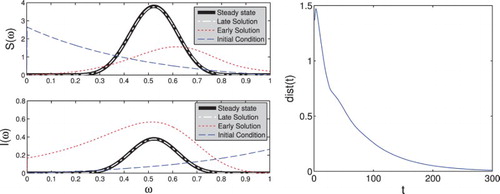
Note that while an order of magnitude apart, the shapes of the steady states for S and I are identical. This is explained by Equation (8(8) $d\left(\omega \right)S\left(\omega \right)+e\left(\omega \right)I\left(\omega \right)=\kappa =\mathrm{const}.$(8) ) (with $\kappa =0$) which yields $S\left(\omega \right)=-\left(e\left(\omega \right)/d\left(\omega \right)\right)I\left(\omega \right)$. In our case $-e\left(\omega \right)/d\left(\omega \right)=10$ from which it follows that the shapes are identical. This is of course a result of our simple choice of parameters and in general this will not be the case.

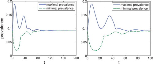
We will use the steady states we found to describe the set $\mathcal{U}$ of possible initial distributions. Namely, we set $\phi \left(\omega \right)=\left(S_{{\theta }^{\ast }}\right(\omega ),I_{{\theta }^{\ast }}(\omega \left)\right)$ and define $\mathcal{U}=\{u\in L_{\mathrm{\infty }}:{\int }_0^{1}u(\omega )\mathrm{d}\omega ={\int }_0^1\phi (\omega )\mathrm{d}\omega ,u(\omega )\in [0.5\phi \left(\omega \right),1.5\phi \left(\omega \right)\left]\right\}.$ Thus, we assume that the prevalence $I\left(t\right)={\int }_0^{1}I(t,\omega )\mathrm{d}\omega$ of the disease is initially as we would expect in a steady state, but we allow uncertainty in the actual distribution of the immune level among the population. That the particular initial condition becomes largely irrelevant for t this large can be seen in Figure 3. There we use the set-membership estimation technique developed in Section 4 to calculate the maximum and minimum value the prevalence $I\left(t\right)$ may achieve. We see that the prevalence converges to a single value independent of the initial condition.

Figure 3. Set-membership estimation of the prevalence $I\left(t\right)$. Note that while for small t the prevalence can take significantly different values for different initial conditions, for large t both the maximum and the minimum converge to the same value. On the right, we show in more detail the interval where the maximum and minimum differ significantly.

We see that with these calculations we can analyse the asymptotic behaviour of the aggregated variables of system (4(4) $\begin{array}{rl}\frac{\mathrm{\partial }}{\mathrm{\partial }t}S(t,\omega )+\frac{\mathrm{\partial }}{\mathrm{\partial }\omega }\left(d\right(\omega \left)S\right(t,\omega \left)\right)& =-\sigma \left(t\right)p\left(\omega \right){\int }_0^{1}q\left(\zeta \right)I(t,\zeta )\mathrm{d}\zeta S(t,\omega )+\delta \left(\omega \right)I(t,\omega ),\\ \frac{\mathrm{\partial }}{\mathrm{\partial }t}I(t,\omega )+\frac{\mathrm{\partial }}{\mathrm{\partial }\omega }\left(e\right(\omega \left)I\right(t,\omega \left)\right)& =\sigma \left(t\right)p\left(\omega \right){\int }_0^{1}q\left(\zeta \right)I(t,\zeta )\mathrm{d}\zeta S(t,\omega )-\delta \left(\omega \right)I(t,\omega ),\end{array}$(4) ). Using the function $r\left(\theta \right)$, we can determine existence and uniqueness of an endemic steady-state solution and using the set-membership estimation, we can conclude that this steady state is globally asymptotically stable for all initial data $u(\cdot )\in \mathcal{U}$.

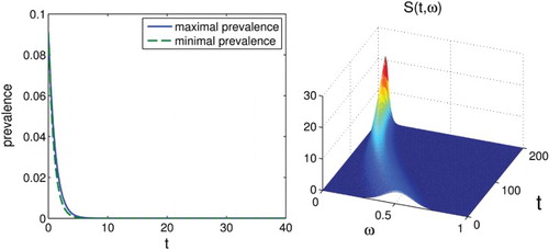
If we significantly decrease the force of infection by taking $\sigma =0.25$, we find that we can no longer find a root of $r\left(\theta \right)$, and numerical calculations yield that $r\left(\theta \right)$ is either plus of minus infinity on the interval $[0,Q]$. In Figure 4, we see that the solution does indeed converge to the disease free steady state, we described in Section 3.

Figure 4. On the left, we show the set-membership estimation of the prevalence for $\sigma =0.25$. It can be seen that the disease dies out. On the right, we show the solution $S(t,\omega )$ with initial condition $u\left(\omega \right)=\phi \left(\omega \right)$. We see that the function does indeed tend towards a Dirac delta at $\omega =0$.

We now calculate solutions to system (4(4) $\begin{array}{rl}\frac{\mathrm{\partial }}{\mathrm{\partial }t}S(t,\omega )+\frac{\mathrm{\partial }}{\mathrm{\partial }\omega }\left(d\right(\omega \left)S\right(t,\omega \left)\right)& =-\sigma \left(t\right)p\left(\omega \right){\int }_0^{1}q\left(\zeta \right)I(t,\zeta )\mathrm{d}\zeta S(t,\omega )+\delta \left(\omega \right)I(t,\omega ),\\ \frac{\mathrm{\partial }}{\mathrm{\partial }t}I(t,\omega )+\frac{\mathrm{\partial }}{\mathrm{\partial }\omega }\left(e\right(\omega \left)I\right(t,\omega \left)\right)& =\sigma \left(t\right)p\left(\omega \right){\int }_0^{1}q\left(\zeta \right)I(t,\zeta )\mathrm{d}\zeta S(t,\omega )-\delta \left(\omega \right)I(t,\omega ),\end{array}$(4) ) with periodic $\sigma \left(t\right)$. We take all parameters as in the previous subsection, but change σ to $\sigma \left(t\right)=2.5(1+\sin (\frac{4\pi }{100}t\left)/100\right)$. The results can be seen in Figure 5. Similar to the case with constant σ the maximal and minimal prevalence converge towards each other. However, they now converge to a periodic solution that oscillates in accordance with the function $\sigma \left(t\right)$. In Figure 6, we show the results if the sinus term is dampened less and we take $\sigma \left(t\right)=2.5(1+\sin (\frac{4\pi }{100}t\left)/10\right)$. 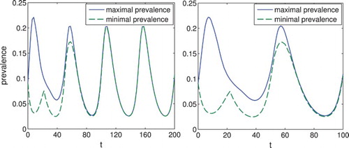Qualitatively, we see the same behaviour as before, but with more pronounced oscillations. Overall we see that periodic behaviour, which is commonly observed in various diseases, is readily reproduced by this model.

Figure 5. Set-estimation of the prevalence for the system with $\sigma \left(t\right)=2.5(1+\sin (\frac{4\pi }{100}t\left)/100\right)$. The prevalence $I\left(t\right)$ converges to a periodic solution.

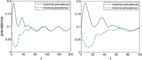
Figure 6. Set-estimation of the prevalence for the system with $\sigma \left(t\right)=2.5(1+\sin (\frac{4\pi }{100}t\left)/10\right)$. The prevalence $I\left(t\right)$ converges again to a periodic solution, but with more pronounced oscillations.

In conclusion, using the techniques developed we are able to estimate the evolution of the disease under uncertain information and to numerically describe the asymptotic behaviour of the system (4(4) $\begin{array}{rl}\frac{\mathrm{\partial }}{\mathrm{\partial }t}S(t,\omega )+\frac{\mathrm{\partial }}{\mathrm{\partial }\omega }\left(d\right(\omega \left)S\right(t,\omega \left)\right)& =-\sigma \left(t\right)p\left(\omega \right){\int }_0^{1}q\left(\zeta \right)I(t,\zeta )\mathrm{d}\zeta S(t,\omega )+\delta \left(\omega \right)I(t,\omega ),\\ \frac{\mathrm{\partial }}{\mathrm{\partial }t}I(t,\omega )+\frac{\mathrm{\partial }}{\mathrm{\partial }\omega }\left(e\right(\omega \left)I\right(t,\omega \left)\right)& =\sigma \left(t\right)p\left(\omega \right){\int }_0^{1}q\left(\zeta \right)I(t,\zeta )\mathrm{d}\zeta S(t,\omega )-\delta \left(\omega \right)I(t,\omega ),\end{array}$(4) ) for initial conditions $u\in \mathcal{U}$. In particular, we see that while the long-term behaviour may be independent of the initial condition u, the short-term behaviour may change significantly for different u. For example, events that decrease the immunity of the population may lead to a temporary outbreak of the disease, or an intervention that is aimed at increasing the immunity will only have temporary benefits. Using set-estimation we can gain information about possible outcomes of such events and actions.

6. Conclusions

In this paper we present a model for the evolution of an infectious disease in a population where the individuals have different immunity and their immune states vary with the time according to its own dynamics. We propose a set-membership estimation procedure based on the available information about the initial distribution of the population along the possible immune states. The rest of the parameters of the model are assumed known. However, this is usually not the case: many of the parameters may be uncertain and changing with the time – the rates of loosing/gaining immunity, d and e, the strength of infection, σ, etc. The approach in this paper can be enhanced correspondingly, with the difference that the auxiliary optimization problems that are involved in the set-membership estimations will become more complex, still being tractable by standard methods in the optimal control theory of size-structured systems (see, e.g. [24]). Such an enhancement could be a topic of further research.

Disclosure statement

No potential conflict of interest was reported by the authors.

Additional information

Funding

This research was supported by the Austrian Science Foundation (FWF) under grant [P 24125-N13].

Appendix

Lemma A.1.

There exists a constant C such that for every $u_1,u_2\in \mathcal{U}$ and for the corresponding solutions $\left(x\right[u_1],y[u_1\left]\right)$ and $\left(x\right[u_2],y[u_2\left]\right)$ of system (16(14) $I_{\theta }^{\prime }\left(\omega \right)=-\frac{\sigma p\left(\omega \right){\int }_0^{1}q\left(\zeta \right)I_{\theta }\left(\zeta \right)\mathrm{d}\zeta }{d\left(\omega \right)}{I}_{\theta }\left(\omega \right)-\frac{\delta \left(\omega \right)+e^{\prime }\left(\omega \right)}{e\left(\omega \right)}{I}_{\theta }\left(\omega \right).$(14) )–(18(15) $r\left(\theta \right)={\int }_0^1((1-\frac{e\left(\omega \right)}{d\left(\omega \right)})\theta -q(\omega \left)\right){\mathrm{e}}^{-{\int }_{{\omega }^{\ast }}^{\omega }\frac{\sigma p\left(\zeta \right)\theta }{d\left(\zeta \right)}+\frac{\delta \left(\zeta \right)+e^{\prime }\left(\zeta \right)}{e\left(\zeta \right)}\mathrm{d}\zeta }\mathrm{d}\omega .$(15) ) it holds that $\parallel x\left[u_1\right]-x\left[u_2\right]{\parallel }_{L_{\mathrm{\infty }}}+\parallel y\left[u_1\right]-y\left[u_2\right]{\parallel }_C\le C\parallel u_1-u_2{\parallel }_{L_{\mathrm{\infty }}}.$

Proof.

According to the definition of a solution, $x_i\left[u_j\right](t,\omega )=z_i\left[u_j\right](t,{\rho }_i(t,\omega \left)\right)$, where $z_i\left[u_j\right]$ together with $y\left[u_j\right]$ satisfy Equations (19(16) $\begin{array}{rl}\frac{\mathrm{\partial }}{\mathrm{\partial }t}x(t,\omega )+\frac{\mathrm{\partial }}{\mathrm{\partial }\omega }\left(A\right(\omega \left)x\right(t,\omega \left)\right)& =f(t,\omega ,x(t,\omega ),y(t\left)\right),x(0,\omega )=u\left(\omega \right),\end{array}$(16) ) and (20(20) $\begin{array}{rl}{z}_i(0,\rho )& =u\left(\rho \right).\end{array}$(20) ) with $u=u_j$, j=1,2. Then, it is straightforward that $\parallel x\left[u_1\right]-x\left[u_2\right]{\parallel }_{L_{\mathrm{\infty }}}=\parallel \mathrm{\Delta }z{\parallel }_{L_{\mathrm{\infty }}},$ where $\mathrm{\Delta }{z}_i(t,\rho )=z_i\left[u_1\right](t,\rho )-z_i\left[u_2\right](t,\rho )$, $\mathrm{\Delta }z=(\mathrm{\Delta }{z}_1,\dots ,{\mathrm{\Delta }}_n)$.

Let $\mathrm{\Theta }\subset [0,1]$ be of full measure and such that the functions $z_i\left[u_j\right](\cdot ,\rho )$ are absolutely continuous for every $\rho \in \mathrm{\Theta }$. Then $\parallel \mathrm{\Delta }z{\parallel }_{L_{\mathrm{\infty }}}=\underset{t\in [0,T]}{sup}\overline{\mathrm{\Delta }z}\left(t\right),$ where $\overline{\mathrm{\Delta }z}\left(t\right):=\underset{i=1,\dots ,n}{max}\underset{\rho \in \mathrm{\Theta }}{sup}|\mathrm{\Delta }{z}_i(t,\rho )|$ is a Lipschitz continuous function due to the uniform Lipschitz continuity of $\mathrm{\Delta }{z}_i(\cdot ,\rho )$. From the assumptions about the data of the system, Equations (17(17) $\begin{array}{rl}y\left(t\right)& ={\int }_0^{1}g(t,\omega ,x(t,\omega \left)\right)\mathrm{d}\omega .\end{array}$(17) ) and (19(16) $\begin{array}{rl}\frac{\mathrm{\partial }}{\mathrm{\partial }t}x(t,\omega )+\frac{\mathrm{\partial }}{\mathrm{\partial }\omega }\left(A\right(\omega \left)x\right(t,\omega \left)\right)& =f(t,\omega ,x(t,\omega ),y(t\left)\right),x(0,\omega )=u\left(\omega \right),\end{array}$(16) ), we successively obtain that $\begin{array}{rl}|y\left[u_1\right]\left(t\right)-y\left[u_2\right]\left(t\right)|& \le c_1\overline{\mathrm{\Delta }z}\left(t\right),\\ \overline{\mathrm{\Delta }z}\left(t\right)& \le \parallel u_1-u_2{\parallel }_{L_{\mathrm{\infty }}}+{\int }_0^t\left(c_2\overline{\mathrm{\Delta }z}\right(s)+c_3|y[u_1\left]\right(s)-y[u_2\left]\right(s\left)|\right))\mathrm{d}s\\ & \le \parallel u_1-u_2{\parallel }_{L_{\mathrm{\infty }}}+{\int }_0^t{c}_4\overline{\mathrm{\Delta }z}\left(s\right)\mathrm{d}s,\end{array}$ where $c_1,\dots ,c_4$ are appropriate constants. The claim of the lemma follows from Grönwall's inequality.

Proof.

Proof of Theorem 4.1 Let $u\in \mathcal{U}$ and let $\tilde{u}\in L_{\mathrm{\infty }}(0,1)$. Denote $\epsilon :=\parallel \tilde{u}-u{\parallel }_{\mathrm{\infty }}$, which will be presumably a ‘small’ number. We denote by $(x,y)$ and $(\tilde{x},\tilde{y})$ the corresponding solutions of Equations (16(14) $I_{\theta }^{\prime }\left(\omega \right)=-\frac{\sigma p\left(\omega \right){\int }_0^{1}q\left(\zeta \right)I_{\theta }\left(\zeta \right)\mathrm{d}\zeta }{d\left(\omega \right)}{I}_{\theta }\left(\omega \right)-\frac{\delta \left(\omega \right)+e^{\prime }\left(\omega \right)}{e\left(\omega \right)}{I}_{\theta }\left(\omega \right).$(14) )–(18(15) $r\left(\theta \right)={\int }_0^1((1-\frac{e\left(\omega \right)}{d\left(\omega \right)})\theta -q(\omega \left)\right){\mathrm{e}}^{-{\int }_{{\omega }^{\ast }}^{\omega }\frac{\sigma p\left(\zeta \right)\theta }{d\left(\zeta \right)}+\frac{\delta \left(\zeta \right)+e^{\prime }\left(\zeta \right)}{e\left(\zeta \right)}\mathrm{d}\zeta }\mathrm{d}\omega .$(15) ). Also we denote by $z_i$ and ${\tilde{z}}_i$ the corresponding z-functions from the definition of a solution, so that $x_i(t,{\omega }_i(t,\rho \left)\right)=z_i(t,\rho )$, similarly for ${\tilde{z}}_i$. Further, $\mathrm{\Delta }u:=\tilde{u}-u$, $\mathrm{\Delta }x:=\tilde{x}-x$, $\mathrm{\Delta }y:=\tilde{y}-y$, and $\mathrm{\Delta }z:=\tilde{z}-z$. Then using Equation (19(16) $\begin{array}{rl}\frac{\mathrm{\partial }}{\mathrm{\partial }t}x(t,\omega )+\frac{\mathrm{\partial }}{\mathrm{\partial }\omega }\left(A\right(\omega \left)x\right(t,\omega \left)\right)& =f(t,\omega ,x(t,\omega ),y(t\left)\right),x(0,\omega )=u\left(\omega \right),\end{array}$(16) ), Lemma A.1 and some standard calculus we obtain that the following equations are fulfilled: $\begin{array}{rl}\frac{\mathrm{d}}{\mathrm{d}t}\mathrm{\Delta }{z}_i(t,\rho )& =f_{ix}(t,{\omega }_i(t,\rho \left)\right)\mathrm{\Delta }x(t,{\omega }_i(t,\rho \left)\right)+f_{iy}(t,{\omega }_i(t,\rho \left)\right)\mathrm{\Delta }y\left(t\right)-a^{\prime }\left({\omega }_i\right(t,\rho \left)\right)\mathrm{\Delta }{z}_i(t,\rho )+o\left(\epsilon \right),\\ \mathrm{\Delta }{z}_i(0,\rho )& =\mathrm{\Delta }{u}_i\left(\rho \right),\\ \mathrm{\Delta }y\left(t\right)& ={\int }_0^1{g}_x(t,\omega ,x(t,\omega \left)\right)\mathrm{\Delta }x(t,\omega )\mathrm{d}\omega +o\left(\epsilon \right),\end{array}$ where the superscripts x and y denote differentiation with respect to x and y, the prime in $a^{\prime }$ denotes differentiation in ω, the missing arguments of $f_{ix}$ and $f_{iy}$ are obviously $x(t,{\omega }_i(t,\rho \left)\right),y\left(t\right)$, and $o\left(\epsilon \right)$ is any function of ϵ (possibly depending on t and ρ), such that $o\left(\epsilon \right)/\epsilon \to 0$ (uniformly in $t,\rho$) when $\epsilon \to 0$. We mention that the second equation above holds due to $z_i(0,\rho )=x_i(0,{\omega }_i(0,\rho \left)\right)=x_i(0,\rho )=u_i\left(\rho \right)$.

Now, we consider the adjoint system (22(18) $x(0,\omega )=u\left(\omega \right),\omega \in [0,1],$(18) ) and denote by ${\zeta }_i(t,\rho )={\lambda }_i(t,{\omega }_i(t,\rho \left)\right),$ the function corresponding to λ in Definition 4.1. Thus $\begin{array}{rl}\frac{\mathrm{d}}{\mathrm{d}t}{\zeta }_i(t,\rho )& =-f_{x_i}(t,{\omega }_i(t,\rho \left){)}^{\ast }\lambda \right(t,{\omega }_i(t,\rho ))-g_{x_i}(t,{\omega }_i(t,\rho ),x(t,{\omega }_i(t,\rho \left)\right){)}^{\ast }\nu \left(t\right),\\ {\zeta }_i(T,\rho )& =-g_{x_i}(T,{\omega }_i(T,\rho ),x(T,{\omega }_i(T,\rho )){)}^{\ast }l,\\ \nu \left(t\right)& ={\int }_0^1{f}_y(t,\omega ,x(t,\omega ),y(t\left){)}^{\ast }\lambda \right(t,\omega )\mathrm{d}\omega .\end{array}$ Using the second last equation and changing the variable $\omega ={\omega }_i(t,\rho )$, we represent (A1) $\begin{array}{rl}{J}_l\left(\tilde{u}\right)-J_l\left(u\right)& =⟨l,\mathrm{\Delta }y\left(T\right)⟩={\int }_0^1⟨l,g_x(T,\omega ,x(T,\omega \left)\right)\mathrm{\Delta }x(T,\omega )⟩\mathrm{d}\omega +o\left(\epsilon \right)\\ & ={\int }_0^1\sum _{i=1}^n\mathrm{\Delta }{x}_i(T,{\omega }_i(T,\rho \left)\right)g_{x_i}(T,{\omega }_i(T,\rho ),x(T,{\omega }_i(T,\rho )\left){)}^{\ast }l\frac{\mathrm{\partial }}{\mathrm{\partial }\rho }{\omega }_i\right(T,\rho )\mathrm{d}\rho +o(\epsilon )\\ & =-\sum _{i=1}^n{\int }_0^1\mathrm{\Delta }{z}_i(T,\rho ){\zeta }_i(T,\rho )\frac{\mathrm{\partial }}{\mathrm{\partial }\rho }{\omega }_i(T,\rho )\mathrm{d}\rho +o\left(\epsilon \right).\end{array}$(A1)

Now, we rework the following expression integrating by parts: $\begin{array}{rl}& \sum _{i=1}^n{\int }_0^T{\int }_0^1\frac{\mathrm{d}}{\mathrm{d}t}\mathrm{\Delta }{z}_i(t,\rho ){\zeta }_i(t,\rho )\frac{\mathrm{\partial }}{\mathrm{\partial }\rho }{\omega }_i(t,\rho )\mathrm{d}\rho \mathrm{d}t\\ & =\sum _{i=1}^n{\int }_0^1\mathrm{\Delta }{z}_i(T,\rho ){\zeta }_i(T,\rho )\frac{\mathrm{\partial }}{\mathrm{\partial }\rho }{\omega }_i(T,\rho )\mathrm{d}\rho -\sum _{i=1}^n{\int }_0^1\mathrm{\Delta }{z}_i(0,\rho ){\zeta }_i(0,\rho )\frac{\mathrm{\partial }}{\mathrm{\partial }\rho }{\omega }_i(0,\rho )\mathrm{d}\rho \\ & -\sum _{i=1}^n{\int }_0^T{\int }_0^1\mathrm{\Delta }{z}_i(t,\rho )\left[\frac{\mathrm{d}}{\mathrm{d}t}{\zeta }_i\right(t,\rho \left)\frac{\mathrm{\partial }}{\mathrm{\partial }\rho }{\omega }_i\right(t,\rho )+{\zeta }_i(t,\rho \left)\frac{\mathrm{\partial }}{\mathrm{\partial }t}\frac{\mathrm{\partial }}{\mathrm{\partial }\rho }{\omega }_i\right(t,\rho \left)\right]\mathrm{d}\rho \mathrm{d}t.\end{array}$ Then, we use the relation (A1(A1) $\begin{array}{rl}{J}_l\left(\tilde{u}\right)-J_l\left(u\right)& =⟨l,\mathrm{\Delta }y\left(T\right)⟩={\int }_0^1⟨l,g_x(T,\omega ,x(T,\omega \left)\right)\mathrm{\Delta }x(T,\omega )⟩\mathrm{d}\omega +o\left(\epsilon \right)\\ & ={\int }_0^1\sum _{i=1}^n\mathrm{\Delta }{x}_i(T,{\omega }_i(T,\rho \left)\right)g_{x_i}(T,{\omega }_i(T,\rho ),x(T,{\omega }_i(T,\rho )\left){)}^{\ast }l\frac{\mathrm{\partial }}{\mathrm{\partial }\rho }{\omega }_i\right(T,\rho )\mathrm{d}\rho +o(\epsilon )\\ & =-\sum _{i=1}^n{\int }_0^1\mathrm{\Delta }{z}_i(T,\rho ){\zeta }_i(T,\rho )\frac{\mathrm{\partial }}{\mathrm{\partial }\rho }{\omega }_i(T,\rho )\mathrm{d}\rho +o\left(\epsilon \right).\end{array}$(A1) ) and the identities $\begin{array}{rl}& \mathrm{\Delta }{z}_i(0,\rho )=\mathrm{\Delta }{u}_i\left(\rho \right),{\zeta }_i(0,\rho )={\zeta }_i(0,{\rho }_i(0,\rho \left)\right)={\lambda }_i(0,\rho ),\\ & \frac{\mathrm{\partial }}{\mathrm{\partial }\rho }{\omega }_i(0,\rho )=1,\frac{\mathrm{\partial }}{\mathrm{\partial }t}\frac{\mathrm{\partial }}{\mathrm{\partial }\rho }{\omega }_i(t,\rho )=a^{\prime }\left({\omega }_i\right(t,\rho \left)\right)\frac{\mathrm{\partial }}{\mathrm{\partial }\rho }{\omega }_i(t,\rho )\end{array}$ to obtain the representation (A2) $J_l\left(\tilde{u}\right)-J_l\left(u\right)=\sum _{i=1}^n{\int }_0^1\mathrm{\Delta }{z}_i(0,\rho ){\zeta }_i(0,\rho )\mathrm{d}\rho +\mathrm{\Delta }+o\left(\epsilon \right)=-{\int }_0^1⟨\lambda (0,\rho ),\mathrm{\Delta }u\left(\rho \right)⟩\mathrm{d}\rho +\mathrm{\Delta }+o\left(\epsilon \right),$(A2) where $\begin{array}{rl}\mathrm{\Delta }& :=-\sum _{i=1}^n{\int }_0^T{\int }_0^1\frac{\mathrm{d}}{\mathrm{d}t}\mathrm{\Delta }{z}_i(t,\rho ){\zeta }_i(t,\rho )\frac{\mathrm{\partial }}{\mathrm{\partial }\rho }{\omega }_i(t,\rho )\mathrm{d}\rho \mathrm{d}t\\ & -\sum _{i=1}^n{\int }_0^T{\int }_0^1\mathrm{\Delta }{z}_i(t,\rho )\left[\frac{\mathrm{d}}{\mathrm{d}t}{\zeta }_i\right(t,\rho )+{\zeta }_i(t,\rho \left)a^{\prime }\right({\omega }_i(t,\rho )\left)\right]\frac{\mathrm{\partial }}{\mathrm{\partial }\rho }{\omega }_i(t,\rho )\mathrm{d}\rho \mathrm{d}t.\end{array}$ After substituting the expressions for $\left(\mathrm{d}/\mathrm{d}t\right)\mathrm{\Delta }{z}_i(t,\rho )$, $\left(\mathrm{d}/\mathrm{d}t\right){\zeta }_i(t,\rho )$, obtained in the beginning of the proof, changing back the variable $\rho ={\omega }_i(t,\omega )$, and using the equations for $\mathrm{\Delta }y$ and ν, it is a matter of simple algebra to obtain that $\mathrm{\Delta }=o\left(\epsilon \right)$. Then from Equation (A2(A2) $J_l\left(\tilde{u}\right)-J_l\left(u\right)=\sum _{i=1}^n{\int }_0^1\mathrm{\Delta }{z}_i(0,\rho ){\zeta }_i(0,\rho )\mathrm{d}\rho +\mathrm{\Delta }+o\left(\epsilon \right)=-{\int }_0^1⟨\lambda (0,\rho ),\mathrm{\Delta }u\left(\rho \right)⟩\mathrm{d}\rho +\mathrm{\Delta }+o\left(\epsilon \right),$(A2) ) $J_l\left(\tilde{u}\right)-J_l\left(u\right)=-{\int }_0^1⟨\lambda (0,\omega ),\tilde{u}\left(\omega \right)-u\left(\omega \right)⟩\mathrm{d}\rho +o(\parallel \tilde{u}-u{\parallel }_{\mathrm{\infty }}),$ which implies the claim of the theorem.

References

- S. Alizon and M. van Baalen, Multiple infections, immune dynamics, and the evolution of virulence, Am. Nat. 172(4) (2008), pp. E150–E168. doi: 10.1086/590958
- L.T.T. An, W. Jäger, and M. Neuss-Radu, Systems of populations with multiple structures: Modeling and analysis, J. Dyn. Diff. Equat. 27 (2015), pp. 863–877. doi: 10.1007/s10884-015-9469-3
- J.B. André, J.B. Ferdy, and B. Godelle, Within-host parasite dynamics, emerging trade-off, and evolution of virulence with immune system, Evolution 57(7) (2003), pp. 1489–1497. doi: 10.1111/j.0014-3820.2003.tb00357.x
- F. Brauer and C. Castillo-Chavez, Mathematical Models in Population Biology and Epidemiology, Springer, New York, 2011.
- M.V. Barbarossa and G. Röst, Immuno-epidemiology of a population structured by immune status: A mathematical study of waning immunity and immune system boosting, J. Math. Biol. 71(6) (2015), pp. 1737–1770. doi: 10.1007/s00285-015-0880-5
- S. Bhattacharya and F.R. Adler, A time since recovery model with varying rates of loss of immunity, Bull. Math. Biol. 74(12) (2012), pp. 2810–2819. doi: 10.1007/s11538-012-9780-7
- T. Day and S.R. Proulx, A general theory for the evolutionary dynamics of virulence, Am. Nat. 163(4) (2004), pp. E40–E63. doi: 10.1086/382548
- O. Diekmann, H. Heesterbeek, and T. Britton, Mathematical Tools for Understanding Infectious Disease Dynamics, Princeton University Press, Princeton, 2012.
- V.V. Ganusov, C.T. Bergstrom, and R. Antia, Within-host population dynamics and the evolution of microparasites in a heterogeneous host population, Evolution 56(2) (2002), pp. 213–223. doi: 10.1111/j.0014-3820.2002.tb01332.x
- M.A. Gilchrist and A. Sasaki, Modeling host-parasite coevolution: A nested approach based on mechanistic models, J. Theoret. Biol. 218(3) (2002), pp. 289–308. doi: 10.1006/jtbi.2002.3076
- B. Hellriegel, Immunoepidemiology – bridging the gap between immunology and epidemiology, Trends Paras. 17(2) (2001), pp. 102–106. doi: 10.1016/S1471-4922(00)01767-0
- H.W. Hethcote, H.W. Stech, and P. Van Den Driessche, Nonlinear oscillations in epidemic models, SIAM J. Appl. Math. 40(1) (1981), pp. 1–9. doi: 10.1137/0140001
- R.I. Hickson and M.G. Roberts, How population heterogeneity in susceptibility and infectivity influences epidemic dynamics, J. Theoret. Biol. 350 (2014), pp. 70–80. doi: 10.1016/j.jtbi.2014.01.014
- W.O. Kermack and A.G. McKendrick, A contribution to the mathematical theory of epidemics, Proc. R. Soc. A: Math., Phys. Eng. Sci. 115 (1927), pp. 700–721. doi: 10.1098/rspa.1927.0118
- A.B. Kurzhanski and P. Varaiya, Dynamics and Control of Trajectory Tubes. Theory and Computation, Systems & Control: Foundations & Applications, Birkhäuser/Springer, Cham, 2014.
- A.B. Kurzhanski and V.M. Veliov (eds.), Modeling Techniques for Uncertain Systems, Progress in Systems and Control Theory 18, Birkhäuser, Boston, MA, 1994.
- M. Milanese, J. Norton, H. Piet-Lahanier, and É. Walter (eds.), Bounding Approaches to System Identification, Plenum Press, New York, 1996.
- J. Mossong, D.J. Nokes, W.J. Edmunds, M.J. Cox, S. Ratnam, and C.P. Muller, Modeling the impact of subclinical measles transmission in vaccinated populations with waning immunity, Am. J. Epidemiol. 150(11) (1999), pp. 1238–1249. doi: 10.1093/oxfordjournals.aje.a009951
- M. Martcheva and S.S. Pilyugin, An epidemic model structured by host immunity, J. Biol. Syst. 14(02) (2006), pp. 185–203. doi: 10.1142/S0218339006001787
- A.S. Perelson and G. Weisbuch, Immunology for physicists, Rev. Mod. Phys. 69(4) (1997), pp. 1219–1268. doi: 10.1103/RevModPhys.69.1219
- V. Rouderfer, N.G. Becker, and H.W. Hethcote, Waning immunity and its effects on vaccination schedules, Math. Biosci. 124(1) (1994), pp. 59–82. doi: 10.1016/0025-5564(94)90024-8
- H.R. Thieme and P. Van Den Driessche, Global stability in cyclic epidemic models with disease fatalities (Proceedings of the conference on Differential Equations with Applications to Biology), Fields. Instit. Commun. 21 (1999), pp. 459–472.
- Ts. Tsachev, V.M. Veliov, and A. Widder, Set-membership estimations for the evolution of infectious diseases in heterogeneous populations. Submitted. Available as Research Report 2015-11, ORCOS, TU Wien, 2015. Available at http://orcos.tuwien.ac.at/research/research_reports.
- V.M. Veliov, Optimal control of heterogeneous systems: Basic theory, J. Math. Anal. Appl. 346 (2008), pp. 227–242. doi: 10.1016/j.jmaa.2008.05.012
- V.M. Veliov, Numerical approximations in optimal control of a class of heterogeneous systems, Comput. Math. Appl. 70(11) (2015), pp. 2652–2660. doi: 10.1016/j.camwa.2015.04.029
- L.J. White and G.F. Medley, Microparasite population dynamics and continuous immunity, Proc. R. Soc. B: Biological Sciences 265(1409) (1998), pp. 1977–1983. doi: 10.1098/rspb.1998.0528
Appendix
Lemma A.1.
There exists a constant C such that for every and for the corresponding solutions
and
of system (Equation16
(14)
(14) )–(Equation18
(15)
(15) ) it holds that
Proof.
According to the definition of a solution, , where
together with
satisfy Equations (Equation19
(16)
(16) ) and (Equation20
(20)
(20) ) with
, j=1,2. Then, it is straightforward that
where
,
.
Let be of full measure and such that the functions
are absolutely continuous for every
. Then
is a Lipschitz continuous function due to the uniform Lipschitz continuity of
. From the assumptions about the data of the system, Equations (Equation17
(17)
(17) ) and (Equation19
(16) ), we successively obtain that
are appropriate constants. The claim of the lemma follows from Grönwall's inequality.
Proof of Theorem 4.1 Let and let
. Denote
, which will be presumably a ‘small’ number. We denote by
the corresponding solutions of Equations (Equation16
(15) ). Also we denote by
the corresponding z-functions from the definition of a solution, so that
, similarly for
. Further,
, and
. Then using Equation (Equation19
(16) ), Lemma A.1 and some standard calculus we obtain that the following equations are fulfilled:
where the superscripts x and y denote differentiation with respect to x and y, the prime in
denotes differentiation in ω, the missing arguments of
are obviously
is any function of ϵ (possibly depending on t and ρ), such that
(uniformly in
) when
. We mention that the second equation above holds due to
Now, we consider the adjoint system (Equation22(18)
(18) ) and denote by
the function corresponding to λ in Definition 4.1. Thus
Using the second last equation and changing the variable