Dual role of delay effects in a tumour–immune system

ABSTRACT

In this paper, a previous tumour–immune interaction model is simplified by neglecting a relatively weak direct immune activation by the tumour cells, which can still keep the essential dynamics properties of the original model. As the immune activation process is not instantaneous, we now incorporate one delay for the activation of the effector cells (ECs) by helper T cells (HTCs) into the model. Furthermore, we investigate the stability and instability regions of the tumour-presence equilibrium state of the delay-induced system with respect to two parameters, the activation rate of ECs by HTCs and the HTCs stimulation rate by the presence of identified tumour antigens. We show the dual role of this delay that can induce stability switches exhibiting destabilization as well as stabilization of the tumour-presence equilibrium. Besides, our results reveal that an appropriate immune activation time delay plays a significant role in control of tumour growth.

KEYWORDS:

• Tumour–immune system
• time delay
• Hopf bifurcation
• destabilization and stabilization

AMS SUBJECT CLASSIFICATION:

• 92D25
• 34C23

1. Introduction

The word ‘tumour’ in reality expresses an entire and wide family of high-mortality pathologies of cellular proliferation which may cause diseases eventually [9]. The immune system is a complicated network of cells and signals that has evolved to protect the host from pathogens and body from tumour cells (TCs). Any new substance in the body that the immune system does not recognize can raise an alarm and cause the immune system to attack it. Sometimes the immune system can recognize TCs, but the response might not be strong and prompt enough to destroy TCs [5]. Effector cells (ECs) are the activated immune system cells, such as cytotoxic T lymphocytes (CTLs) [15]. TCs are mainly the prey of the ECs, on the other hand, proliferation of ECs is stimulated by the existence of TCs. However, TCs also cause a loss of ECs, and intensity of an influx of ECs may rely on the size of the tumour  [8]. Helper T cells (HTCs) are stimulated through antigen presentation by macrophages or dendritic cells and release the cytokines to stimulate proliferation of ECs to kill more TCs. The tumour–immune competitive system is complicated, being nonlinear and evolutive in some extent [10].

To capture the dynamics of tumour–immune system interaction, a lot of mathematical efforts have been made [1–4, 6–11, 13–20]. For example, a classical model describing the CTL response to the growth of an immunogenic tumour was presented in [16]. Kirschner et al. first introduced immunotherapy into their models which can explain both short-term tumour oscillations in tumour sizes and long-term tumour relapse [15]. d'Onofrio et al. [8] introduced a general framework for modelling tumour–immune system competition and immunotherapy using the qualitative theory of differential equations. de Pillis et al. [3] proposed a mathematical model of tumour–immune interaction with chemotherapy and strategies for optimally administering treatment. Recently, Dong et al. [7] studied the role of HTCs in the tumour–immune system: (1) $\begin{array}{rl}\frac{\mathrm{d}T\left(t\right)}{\mathrm{d}t}& =aT\left(t\right)(1-bT(t\left)\right)-nE\left(t\right)T\left(t\right),\\ \frac{\mathrm{d}E\left(t\right)}{\mathrm{d}t}& =s_1-d_{1}E\left(t\right)+k_{1}T\left(t\right)E\left(t\right)+pE\left(t\right)H\left(t\right),\\ \frac{\mathrm{d}H\left(t\right)}{\mathrm{d}t}& =s_2-d_{2}H\left(t\right)+k_{2}T\left(t\right)H\left(t\right),\end{array}$(1) where $T\left(t\right)$, $E\left(t\right)$ and $H\left(t\right)$ are the densities of TCs, ECs and HTCs , respectively. The logistic term $aT(1-bT)$ describes the growth of TCs, where a denotes the maximal growth rate of the TCs population and $b^{-1}$ denotes the maximal carrying capacity of the biological environment for TCs. n represents the loss rate of TCs by ECs interaction. $s_1$ is referred to as the constant flow rate of mature ECs into the region of TCs localization. ECs have a natural lifespan of an average $1/d_1$ days. $k_1$ is ECs stimulation rate by ECs-lysed TCs debris. p is an activation rate of ECs by HTCs. $s_2$ is referred to as birth rate of HTCs produced in the bone marrow. HTCs have a natural lifespan of an average $1/d_2$ days. $k_2$ is the HTCs stimulation rate by the presence of identified tumour antigens. To consider a weak proliferation of ECs stimulating by TCs, we can simplify this system by ignoring the ECs stimulation from TCs (that is to omit the term $+k_{1}T\left(t\right)E\left(t\right)$ in system (1(1) $\begin{array}{rl}\frac{\mathrm{d}T\left(t\right)}{\mathrm{d}t}& =aT\left(t\right)(1-bT(t\left)\right)-nE\left(t\right)T\left(t\right),\\ \frac{\mathrm{d}E\left(t\right)}{\mathrm{d}t}& =s_1-d_{1}E\left(t\right)+k_{1}T\left(t\right)E\left(t\right)+pE\left(t\right)H\left(t\right),\\ \frac{\mathrm{d}H\left(t\right)}{\mathrm{d}t}& =s_2-d_{2}H\left(t\right)+k_{2}T\left(t\right)H\left(t\right),\end{array}$(1) )), while keeping the essential dynamics properties of the original system. Then, we obtain the simplified system: (2) $\begin{array}{rl}\frac{\mathrm{d}T\left(t\right)}{\mathrm{d}t}& =aT\left(t\right)(1-bT(t\left)\right)-nE\left(t\right)T\left(t\right),\\ \frac{\mathrm{d}E\left(t\right)}{\mathrm{d}t}& =s_1-d_{1}E\left(t\right)+pE\left(t\right)H\left(t\right),\\ \frac{\mathrm{d}H\left(t\right)}{\mathrm{d}t}& =s_2-d_{2}H\left(t\right)+k_{2}T\left(t\right)H\left(t\right),\end{array}$(2) with initial conditions $T\left(0\right)=T_0>0,E\left(0\right)=E_0\ge 0$ and $H\left(0\right)=H_0\ge 0$.

As suggested in [16], we choose the scaling $E_0=T_0=H_0$ to improve the performance of numerical simulations. Then, system (2(2) $\begin{array}{rl}\frac{\mathrm{d}T\left(t\right)}{\mathrm{d}t}& =aT\left(t\right)(1-bT(t\left)\right)-nE\left(t\right)T\left(t\right),\\ \frac{\mathrm{d}E\left(t\right)}{\mathrm{d}t}& =s_1-d_{1}E\left(t\right)+pE\left(t\right)H\left(t\right),\\ \frac{\mathrm{d}H\left(t\right)}{\mathrm{d}t}& =s_2-d_{2}H\left(t\right)+k_{2}T\left(t\right)H\left(t\right),\end{array}$(2) ) can be rescaled by introducing the new variables: $x=T/T_0,y=E/T_0,z=H/T_0,\tau =n{T}_{0}t,\alpha =a/n{T}_0,\beta =b{T}_0,{\sigma }_1=s_1/n{T_0}^2,{\delta }_1=d_1/n{T}_0,\rho =p/n,{\sigma }_2=s_2/n{T_0}^2,\omega =k_2/n,{\delta }_2=d_2/n{T}_0.$ By replacing τ by t, system (2(2) $\begin{array}{rl}\frac{\mathrm{d}T\left(t\right)}{\mathrm{d}t}& =aT\left(t\right)(1-bT(t\left)\right)-nE\left(t\right)T\left(t\right),\\ \frac{\mathrm{d}E\left(t\right)}{\mathrm{d}t}& =s_1-d_{1}E\left(t\right)+pE\left(t\right)H\left(t\right),\\ \frac{\mathrm{d}H\left(t\right)}{\mathrm{d}t}& =s_2-d_{2}H\left(t\right)+k_{2}T\left(t\right)H\left(t\right),\end{array}$(2) ) becomes (3) $\begin{array}{rl}\frac{\mathrm{d}x\left(t\right)}{\mathrm{d}t}& =\alpha x\left(t\right)(1-\beta x(t\left)\right)-x\left(t\right)y\left(t\right),\\ \frac{\mathrm{d}y\left(t\right)}{\mathrm{d}t}& ={\sigma }_1-{\delta }_{1}y\left(t\right)+\rho y\left(t\right)z\left(t\right),\\ \frac{\mathrm{d}z\left(t\right)}{\mathrm{d}t}& ={\sigma }_2-{\delta }_{2}z\left(t\right)+\omega x\left(t\right)z\left(t\right),\end{array}$(3) with initial conditions $x\left(0\right)>0,y\left(0\right)\ge 0$ and $z\left(0\right)\ge 0$, where $x\left(t\right),y\left(t\right)$ and $z\left(t\right)$ denote the dimensionless density of the TCs, ECs and HTCs population, respectively.

In reality, the immune system will take more time to give a suitable response after recognizing the non-self cells. Thus, we need to take into account the effect of time delay to describe the proliferation of ECs stimulating by HTCs. There are mainly two ways to incorporate delay effects into the ordinary differential equations (ODEs) system. One way is to directly introduce a delay term (e.g. $+\rho y\left(t\right)z(t-\theta )$) with $\theta >0$. Following this, Dong et al. [6] constructed the dynamical behaviour of a tumour–immune system interaction model with two discrete delays. And the other way is to introduce a kernel function as an additional compartment. In this study, we use a function $G\left(t\right)={\int }_{-\mathrm{\infty }}^{t}b{e}^{-b(t-s)}z\left(s\right)\mathrm{d}s$ to represent the immune activation delay taking the following form: (4) $\begin{array}{rl}\frac{\mathrm{d}x\left(t\right)}{\mathrm{d}t}& =\alpha x\left(t\right)(1-\beta x(t\left)\right)-x\left(t\right)y\left(t\right),\\ \frac{\mathrm{d}y\left(t\right)}{\mathrm{d}t}& ={\sigma }_1-{\delta }_{1}y\left(t\right)+\rho y\left(t\right)G\left(t\right),\\ \frac{\mathrm{d}z\left(t\right)}{\mathrm{d}t}& ={\sigma }_2-{\delta }_{2}z\left(t\right)+\omega x\left(t\right)z\left(t\right),\\ \frac{\mathrm{d}G\left(t\right)}{\mathrm{d}t}& =bz\left(t\right)-bG\left(t\right),\end{array}$(4) where b is a positive constant expressing the strength of delay. In fact, $G\left(t\right)$ can be rewritten as $G\left(t\right)={\int }_0^{\mathrm{\infty }}b{e}^{-bu}z(t-u)\mathrm{d}u$. Note that $b{e}^{-bu}$ is the weight function for $z(t-u)$ and monotonically decreasing with respect to u. The mean delay of the weight function $b{e}^{-bu}$ is 1/b. Hence, the immune activation depends on the density of HTCs at the present time t when b is large. On the other hand, when b is small, the activation depends also on the density of HTCs at the past time t−u. This study is aimed to investigate the role of delay effects in the tumour–immune system.

The rest of the paper is organized as follows. The stability of tumour-free and tumour-presence equilibria of systems (3(3) $\begin{array}{rl}\frac{\mathrm{d}x\left(t\right)}{\mathrm{d}t}& =\alpha x\left(t\right)(1-\beta x(t\left)\right)-x\left(t\right)y\left(t\right),\\ \frac{\mathrm{d}y\left(t\right)}{\mathrm{d}t}& ={\sigma }_1-{\delta }_{1}y\left(t\right)+\rho y\left(t\right)z\left(t\right),\\ \frac{\mathrm{d}z\left(t\right)}{\mathrm{d}t}& ={\sigma }_2-{\delta }_{2}z\left(t\right)+\omega x\left(t\right)z\left(t\right),\end{array}$(3) ) and (4(4) $\begin{array}{rl}\frac{\mathrm{d}x\left(t\right)}{\mathrm{d}t}& =\alpha x\left(t\right)(1-\beta x(t\left)\right)-x\left(t\right)y\left(t\right),\\ \frac{\mathrm{d}y\left(t\right)}{\mathrm{d}t}& ={\sigma }_1-{\delta }_{1}y\left(t\right)+\rho y\left(t\right)G\left(t\right),\\ \frac{\mathrm{d}z\left(t\right)}{\mathrm{d}t}& ={\sigma }_2-{\delta }_{2}z\left(t\right)+\omega x\left(t\right)z\left(t\right),\\ \frac{\mathrm{d}G\left(t\right)}{\mathrm{d}t}& =bz\left(t\right)-bG\left(t\right),\end{array}$(4) ) was discussed, respectively, in Section 2. The numerical simulations were performed in Section 3. The conclusion and discussion were given in Section 4.

2. Steady states and stability analysis

2.1. Dynamics of system (3)

In order to investigate the steady states of system (3(3) $\begin{array}{rl}\frac{\mathrm{d}x\left(t\right)}{\mathrm{d}t}& =\alpha x\left(t\right)(1-\beta x(t\left)\right)-x\left(t\right)y\left(t\right),\\ \frac{\mathrm{d}y\left(t\right)}{\mathrm{d}t}& ={\sigma }_1-{\delta }_{1}y\left(t\right)+\rho y\left(t\right)z\left(t\right),\\ \frac{\mathrm{d}z\left(t\right)}{\mathrm{d}t}& ={\sigma }_2-{\delta }_{2}z\left(t\right)+\omega x\left(t\right)z\left(t\right),\end{array}$(3) ), we set $\mathrm{d}x/\mathrm{d}t=0,\mathrm{d}y/\mathrm{d}t=0$ and $\mathrm{d}z/\mathrm{d}t=0$, and we have (5) $0=x\left[\alpha \right(1-\beta x)-y],{\sigma }_1=({\delta }_1-\rho z)y,{\sigma }_2=({\delta }_2-\omega x)z.$(5)

Substituting x=0 leads to the tumour-free equilibrium, $E_0=(x_0,y_0,z_0)=\left(0,\frac{{\sigma }_1{\delta }_2}{{\delta }_1{\delta }_2-\rho {\sigma }_2},\frac{{\sigma }_2}{{\delta }_2}\right).$ $E_0$ exists, when $\rho <\left({\delta }_1{\delta }_2/{\sigma }_2\right)\equiv {\rho }_0$.

Next, we consider the existence of tumour-presence equilibrium. Substituting $x\ne 0$ and eliminating z in Equation (5(5) $0=x\left[\alpha \right(1-\beta x)-y],{\sigma }_1=({\delta }_1-\rho z)y,{\sigma }_2=({\delta }_2-\omega x)z.$(5) ) yields $F\left(x\right)=\left(\alpha \beta {\delta }_1\omega \right)x^2+[\omega {\sigma }_1-\alpha {\delta }_1\omega -\alpha \beta ({\delta }_1{\delta }_2-\rho {\sigma }_2\left)\right]x+\alpha ({\delta }_1{\delta }_2-\rho {\sigma }_2)-{\sigma }_1{\delta }_2=0.$

Since $F\left(x\right)=0$ has a positive discriminant $\begin{array}{rl}\mathrm{\Delta }& =[\omega {\sigma }_1-\alpha {\delta }_1\omega -\alpha \beta ({\delta }_1{\delta }_2-\rho {\sigma }_2){]}^2-4(\alpha \beta {\delta }_1\omega \left)\right[\alpha ({\delta }_1{\delta }_2-\rho {\sigma }_2)-{\sigma }_1{\delta }_2]\\ & =\left[\omega \right({\sigma }_1-\alpha {\delta }_1)+\alpha \beta ({\delta }_1{\delta }_2-\rho {\sigma }_2){]}^2+4\alpha \beta \omega \rho {\sigma }_1{\sigma }_2>0,\end{array}$ there exist two solutions $x_1$ and $x_2$ ($x_1<x_2$) to $F\left(x\right)=0$ given by $x_{1,2}=\frac{\alpha \beta ({\delta }_1{\delta }_2-\rho {\sigma }_2)+\alpha {\delta }_1\omega -\omega {\sigma }_1\pm \sqrt{\mathrm{\Delta }}}{2\alpha \beta {\delta }_1\omega }.$

By substituting $1/\beta$ and ${\delta }_2/\omega$ into $F\left(x\right)$, respectively, we have $F\left(1/\beta \right)={\sigma }_1\omega (1/\beta -{\delta }_2/\omega )$ and $F\left({\delta }_2/\omega \right)=\alpha \beta \rho {\sigma }_2({\delta }_2/\omega -1/\beta )$. If $1/\beta <{\delta }_2/\omega$, then $F\left(1/\beta \right)<0$ and $F\left({\delta }_2/\omega \right)>0$, so the larger solution $x_2$ satisfies $1/\beta <x_2<{\delta }_2/\omega$; if $1/\beta >{\delta }_2/\omega$, then $F\left(1/\beta \right)>0$ and $F\left({\delta }_2/\omega \right)<0$, so $x_2$ satisfies $1/\beta >x_2>{\delta }_2/\omega$. In a word, we have $F\left(1/\beta \right)F\left({\delta }_2/\omega \right)=-\alpha \beta \rho \omega {\sigma }_1{\sigma }_2(1/\beta -{\delta }_2/\omega {)}^2<0$ and $x_2>min\left\{{\delta }_2/\omega ,1/\beta \right\}$. However, from Equation (5(5) $0=x\left[\alpha \right(1-\beta x)-y],{\sigma }_1=({\delta }_1-\rho z)y,{\sigma }_2=({\delta }_2-\omega x)z.$(5) ), the tumour-presence equilibrium $x^{\ast }$ must satisfy the conditions $x^{\ast }<1/\beta$ and $x^{\ast }<{\delta }_2/\omega$ to enable that $y^{\ast }>0$ and $z^{\ast }>0$. So $x_2(>min\{{\delta }_2/\omega ,1/\beta \}$) cannot be $x^{\ast }$. The remaining possibility is $x_1=x^{\ast }>0$. If $F\left(0\right)>0$ which equals to $\rho <{\delta }_1{\delta }_2/{\sigma }_2-{\sigma }_1{\delta }_2/\alpha {\sigma }_2\equiv {\rho }_1$, then $F\left(x\right)=0$ has only one positive solution $x^{\ast }=x_1=\alpha \beta ({\delta }_1{\delta }_2-\rho {\sigma }_2)+\alpha {\delta }_1\omega -\omega {\sigma }_1-\sqrt{\mathrm{\Delta }}/2\alpha \beta {\delta }_1\omega$. So, we can conclude that there exists a unique tumour-presence equilibrium $E^{\ast }=(x^{\ast },y^{\ast },z^{\ast })=(x^{\ast },\alpha (1-\beta x^{\ast }),{\sigma }_2/({\delta }_2-\omega x^{\ast }\left)\right)$, when $\rho <{\rho }_1$.

Now, let us study the stability of two equilibria $E_0$ and $E^{\ast }$.

We compute the Jacobian matrix of system (3(3) $\begin{array}{rl}\frac{\mathrm{d}x\left(t\right)}{\mathrm{d}t}& =\alpha x\left(t\right)(1-\beta x(t\left)\right)-x\left(t\right)y\left(t\right),\\ \frac{\mathrm{d}y\left(t\right)}{\mathrm{d}t}& ={\sigma }_1-{\delta }_{1}y\left(t\right)+\rho y\left(t\right)z\left(t\right),\\ \frac{\mathrm{d}z\left(t\right)}{\mathrm{d}t}& ={\sigma }_2-{\delta }_{2}z\left(t\right)+\omega x\left(t\right)z\left(t\right),\end{array}$(3) ) at $E_0$, denoted by $J\left(E_0\right)=\left(\begin{array}{ccc}\alpha -y_0& 0& 0\\ 0& -{\delta }_1+\rho z_0& \rho y_0\\ \omega z_0& 0& -{\delta }_2\end{array}\right).$ The eigenvalues of $J\left(E_0\right)$ are ${\lambda }_1=-{\delta }_2<0,{\lambda }_2=(\rho {\sigma }_2-{\delta }_1{\delta }_2)/{\delta }_2$ and ${\lambda }_3=\alpha -{\sigma }_1{\delta }_2/({\delta }_1{\delta }_2-\rho {\sigma }_2)$. All of the eigenvalues are negative if ${\rho }_1<\rho <{\rho }_0$. Thus, we have the following result.

Theorem 2.1.

The tumour-free equilibrium $E_0$ is locally asymptotically stable if ${\rho }_1<\rho <{\rho }_0$.

The Jacobian matrix of Equation (3(3) $\begin{array}{rl}\frac{\mathrm{d}x\left(t\right)}{\mathrm{d}t}& =\alpha x\left(t\right)(1-\beta x(t\left)\right)-x\left(t\right)y\left(t\right),\\ \frac{\mathrm{d}y\left(t\right)}{\mathrm{d}t}& ={\sigma }_1-{\delta }_{1}y\left(t\right)+\rho y\left(t\right)z\left(t\right),\\ \frac{\mathrm{d}z\left(t\right)}{\mathrm{d}t}& ={\sigma }_2-{\delta }_{2}z\left(t\right)+\omega x\left(t\right)z\left(t\right),\end{array}$(3) ) at $E^{\ast }$ is $J\left(E^{\ast }\right)=\left(\begin{array}{ccc}\alpha -2\alpha \beta x^{\ast }-y^{\ast }& -x^{\ast }& 0\\ 0& -{\delta }_1+\rho z^{\ast }& \rho y^{\ast }\\ \omega z^{\ast }& 0& \omega x^{\ast }-{\delta }_2\end{array}\right).$ The characteristic equation of $J\left(E^{\ast }\right)$ takes the form (6) ${\lambda }^3+b_1{\lambda }^2+b_2\lambda +b_3=0,$(6) where $\begin{array}{rl}{b}_1& =\alpha \beta x^{\ast }+\frac{{\sigma }_1}{y^{\ast }}+\frac{{\sigma }_2}{z^{\ast }}>0,\\ b_2& =\alpha \beta x^{\ast }\frac{{\sigma }_1}{y^{\ast }}+\alpha \beta x^{\ast }\frac{{\sigma }_2}{z^{\ast }}+\frac{{\sigma }_1}{y^{\ast }}\frac{{\sigma }_2}{z^{\ast }}>0,\\ b_3& =\alpha \beta x^{\ast }\frac{{\sigma }_1}{y^{\ast }}\frac{{\sigma }_2}{z^{\ast }}+\rho \omega x^{\ast }{y}^{\ast }{z}^{\ast }>0.\end{array}$ According to the Routh–Hurwitz criterion, we know that all roots of Equation (6(6) ${\lambda }^3+b_1{\lambda }^2+b_2\lambda +b_3=0,$(6) ) have negative real parts if and only if $b_1>0,b_3>0$ and $b_1{b}_2-b_3>0.$ Thus, the sufficient condition for stability of $E^{\ast }$ is given by (7) $\begin{array}{rl}{b}_1{b}_2-b_3& =\left(\alpha \beta x^{\ast }+\frac{{\sigma }_1}{y^{\ast }}\right)\left(\alpha \beta x^{\ast }\frac{{\sigma }_1}{y^{\ast }}+\alpha \beta x^{\ast }\frac{{\sigma }_2}{z^{\ast }}+\frac{{\sigma }_1}{y^{\ast }}\frac{{\sigma }_2}{z^{\ast }}\right)\\ & +\frac{{\sigma }_2}{z^{\ast }}\left(\alpha \beta x^{\ast }\frac{{\sigma }_2}{z^{\ast }}+\frac{{\sigma }_1}{y^{\ast }}\frac{{\sigma }_2}{z^{\ast }}\right)-\rho \omega x^{\ast }{y}^{\ast }{z}^{\ast }>0,\end{array}$(7) where $y^{\ast }=\alpha (1-\beta x^{\ast })$ and $z^{\ast }={\sigma }_2/({\delta }_2-\omega x^{\ast })$. Thus, we have the following result.

Theorem 2.2.

System (3(3) $\begin{array}{rl}\frac{\mathrm{d}x\left(t\right)}{\mathrm{d}t}& =\alpha x\left(t\right)(1-\beta x(t\left)\right)-x\left(t\right)y\left(t\right),\\ \frac{\mathrm{d}y\left(t\right)}{\mathrm{d}t}& ={\sigma }_1-{\delta }_{1}y\left(t\right)+\rho y\left(t\right)z\left(t\right),\\ \frac{\mathrm{d}z\left(t\right)}{\mathrm{d}t}& ={\sigma }_2-{\delta }_{2}z\left(t\right)+\omega x\left(t\right)z\left(t\right),\end{array}$(3) ) has one tumour-presence equilibrium $E^{\ast }$ if $0<\rho <{\rho }_1,$ which is locally asymptotically stable if the inequality in (7(7) $\begin{array}{rl}{b}_1{b}_2-b_3& =\left(\alpha \beta x^{\ast }+\frac{{\sigma }_1}{y^{\ast }}\right)\left(\alpha \beta x^{\ast }\frac{{\sigma }_1}{y^{\ast }}+\alpha \beta x^{\ast }\frac{{\sigma }_2}{z^{\ast }}+\frac{{\sigma }_1}{y^{\ast }}\frac{{\sigma }_2}{z^{\ast }}\right)\\ & +\frac{{\sigma }_2}{z^{\ast }}\left(\alpha \beta x^{\ast }\frac{{\sigma }_2}{z^{\ast }}+\frac{{\sigma }_1}{y^{\ast }}\frac{{\sigma }_2}{z^{\ast }}\right)-\rho \omega x^{\ast }{y}^{\ast }{z}^{\ast }>0,\end{array}$(7) ) holds.

2.2. Dynamics of system (4)

Following the similar analysis of the steady states in system (3(3) $\begin{array}{rl}\frac{\mathrm{d}x\left(t\right)}{\mathrm{d}t}& =\alpha x\left(t\right)(1-\beta x(t\left)\right)-x\left(t\right)y\left(t\right),\\ \frac{\mathrm{d}y\left(t\right)}{\mathrm{d}t}& ={\sigma }_1-{\delta }_{1}y\left(t\right)+\rho y\left(t\right)z\left(t\right),\\ \frac{\mathrm{d}z\left(t\right)}{\mathrm{d}t}& ={\sigma }_2-{\delta }_{2}z\left(t\right)+\omega x\left(t\right)z\left(t\right),\end{array}$(3) ), for system (4(4) $\begin{array}{rl}\frac{\mathrm{d}x\left(t\right)}{\mathrm{d}t}& =\alpha x\left(t\right)(1-\beta x(t\left)\right)-x\left(t\right)y\left(t\right),\\ \frac{\mathrm{d}y\left(t\right)}{\mathrm{d}t}& ={\sigma }_1-{\delta }_{1}y\left(t\right)+\rho y\left(t\right)G\left(t\right),\\ \frac{\mathrm{d}z\left(t\right)}{\mathrm{d}t}& ={\sigma }_2-{\delta }_{2}z\left(t\right)+\omega x\left(t\right)z\left(t\right),\\ \frac{\mathrm{d}G\left(t\right)}{\mathrm{d}t}& =bz\left(t\right)-bG\left(t\right),\end{array}$(4) ) we obtain the tumour-free equilibrium, $E^{-}=(x^{-},y^{-},z^{-},G^{-})=\left(0,\frac{{\sigma }_1{\delta }_2}{{\delta }_1{\delta }_2-\rho {\sigma }_2},\frac{{\sigma }_2}{{\delta }_2},\frac{{\sigma }_2}{{\delta }_2}\right).$ $E^{-}$ exists, when $\rho <\left({\delta }_1{\delta }_2/{\sigma }_2\right)\equiv {\rho }_0$.

And we can also obtain the unique tumour-presence equilibrium $E^{+}=(x^{+},y^{+},z^{+},G^{+})=(x^{+},\alpha (1-\beta x^{+}),{\sigma }_2/{\delta }_2-\omega x^{+},{\sigma }_2/{\delta }_2-\omega x^{+})$, where $x^{+}=\alpha \beta ({\delta }_1{\delta }_2-\rho {\sigma }_2)+\alpha {\delta }_1\omega -\omega {\sigma }_1-\sqrt{\mathrm{\Delta }}/2\alpha \beta {\delta }_1\omega$, when $\rho <{\rho }_1$. Note that $(x^{+},y^{+},z^{+},G^{+})=(x^{\ast },y^{\ast },z^{\ast },z^{\ast })$.

Now, we discuss the stability of two equilibria $E^{-}$ and $E^{+}$ of system (4(4) $\begin{array}{rl}\frac{\mathrm{d}x\left(t\right)}{\mathrm{d}t}& =\alpha x\left(t\right)(1-\beta x(t\left)\right)-x\left(t\right)y\left(t\right),\\ \frac{\mathrm{d}y\left(t\right)}{\mathrm{d}t}& ={\sigma }_1-{\delta }_{1}y\left(t\right)+\rho y\left(t\right)G\left(t\right),\\ \frac{\mathrm{d}z\left(t\right)}{\mathrm{d}t}& ={\sigma }_2-{\delta }_{2}z\left(t\right)+\omega x\left(t\right)z\left(t\right),\\ \frac{\mathrm{d}G\left(t\right)}{\mathrm{d}t}& =bz\left(t\right)-bG\left(t\right),\end{array}$(4) ).

We compute the Jacobian matrix of system (4(4) $\begin{array}{rl}\frac{\mathrm{d}x\left(t\right)}{\mathrm{d}t}& =\alpha x\left(t\right)(1-\beta x(t\left)\right)-x\left(t\right)y\left(t\right),\\ \frac{\mathrm{d}y\left(t\right)}{\mathrm{d}t}& ={\sigma }_1-{\delta }_{1}y\left(t\right)+\rho y\left(t\right)G\left(t\right),\\ \frac{\mathrm{d}z\left(t\right)}{\mathrm{d}t}& ={\sigma }_2-{\delta }_{2}z\left(t\right)+\omega x\left(t\right)z\left(t\right),\\ \frac{\mathrm{d}G\left(t\right)}{\mathrm{d}t}& =bz\left(t\right)-bG\left(t\right),\end{array}$(4) ) at $E^{-}$, denoted by $J\left(E^{-}\right)=\left(\begin{array}{cccc}\alpha -y^{-}& 0& 0& 0\\ 0& -{\delta }_1+\rho G^{-}& 0& \rho y^{-}\\ \omega z^{-}& 0& -{\delta }_2& 0\\ 0& 0& b& -b\end{array}\right).$ The eigenvalues of $J\left(E^{-}\right)$ are ${\lambda }_1=-{\delta }_2<0,{\lambda }_2=(\rho {\sigma }_2-{\delta }_1{\delta }_2)/{\delta }_2,{\lambda }_3=\alpha -{\sigma }_1{\delta }_2/({\delta }_1{\delta }_2-\rho {\sigma }_2),{\lambda }_4=-b<0.$ It can be seen that all the eigenvalues are negative if and only if ${\rho }_1<\rho <{\rho }_0$. Thus, we have the following result.

Theorem 2.3.

The tumour-free equilibrium $E^{-}$ is locally asymptotically stable if ${\rho }_1<\rho <{\rho }_0$.

The Jacobian matrix of system (4(4) $\begin{array}{rl}\frac{\mathrm{d}x\left(t\right)}{\mathrm{d}t}& =\alpha x\left(t\right)(1-\beta x(t\left)\right)-x\left(t\right)y\left(t\right),\\ \frac{\mathrm{d}y\left(t\right)}{\mathrm{d}t}& ={\sigma }_1-{\delta }_{1}y\left(t\right)+\rho y\left(t\right)G\left(t\right),\\ \frac{\mathrm{d}z\left(t\right)}{\mathrm{d}t}& ={\sigma }_2-{\delta }_{2}z\left(t\right)+\omega x\left(t\right)z\left(t\right),\\ \frac{\mathrm{d}G\left(t\right)}{\mathrm{d}t}& =bz\left(t\right)-bG\left(t\right),\end{array}$(4) ) at $E^{+}$ is $J\left(E^{+}\right)=\left(\begin{array}{cccc}\alpha -2\alpha \beta x^{+}-y^{+}& -x^{+}& 0& 0\\ 0& -{\delta }_1+\rho G^{+}& 0& \rho y^{+}\\ \omega z^{+}& 0& \omega x^{+}-{\delta }_2& 0\\ 0& 0& b& -b\end{array}\right).$ The characteristic equation of $J\left(E^{+}\right)$ takes the form (8) ${\lambda }^4+B_1{\lambda }^3+B_2{\lambda }^2+B_3\lambda +B_4=0,$(8) where $B_1=b+b_1>0,B_2=b{b}_1+b_2>0,B_3=b{b}_2+b_3-b_4>0,B_4=b{b}_3>0,$ while $b_1>0$, $b_2>0$ and $b_3>0$ are defined in Equation (6(6) ${\lambda }^3+b_1{\lambda }^2+b_2\lambda +b_3=0,$(6) ) and $b_4=\rho \omega x^{+}{y}^{+}{z}^{+}$. Note that $b_3-b_4=\alpha \beta x^{+}\left({\sigma }_1/y^{+}\right)\left({\sigma }_2/z^{+}\right)>0$. According to the Routh–Hurwitz criterion, we know that all roots of Equation (8(8) ${\lambda }^4+B_1{\lambda }^3+B_2{\lambda }^2+B_3\lambda +B_4=0,$(8) ) have negative real parts if and only if $B_1>0$, $B_1{B}_2-B_3>0$, $(B_1{B}_2-B_3)B_3-B_1^2{B}_4>0$ and $\left[\right(B_1{B}_2-B_3)B_3-B_1^2{B}_4]B_4>0.$

It is easy to check that $B_1>0$, $B_4>0$. Further we can check that $B_1{B}_2-B_3>0$. In fact, $B_1{B}_2-B_3=b_1{b}^2+b_1^{2}b+b_1{b}_2-b_3+b_4>0$, since $b_1{b}_2-b_3+b_4>0$ by the definition (6(6) ${\lambda }^3+b_1{\lambda }^2+b_2\lambda +b_3=0,$(6) ). Thus, the sufficient condition for stability of $E^{+}$ is given by $(B_1{B}_2-B_3)B_3-B_1^2{B}_4=P_3{b}^3+P_2{b}^2+P_{1}b+P_0\triangleq Q\left(b\right)>0,$ where $\begin{array}{rl}{P}_3& =b_1{b}_2-b_3,\\ P_2& =b_1(b_1{b}_2-b_3-b_4),\\ P_1& =b_2(b_1{b}_2-b_3)+b_4(b_2-b_1^2),\\ P_0& =(b_3-b_4)(b_1{b}_2-b_3+b_4).\end{array}$ Thus, we have the following result.

Theorem 2.4.

System (4(4) $\begin{array}{rl}\frac{\mathrm{d}x\left(t\right)}{\mathrm{d}t}& =\alpha x\left(t\right)(1-\beta x(t\left)\right)-x\left(t\right)y\left(t\right),\\ \frac{\mathrm{d}y\left(t\right)}{\mathrm{d}t}& ={\sigma }_1-{\delta }_{1}y\left(t\right)+\rho y\left(t\right)G\left(t\right),\\ \frac{\mathrm{d}z\left(t\right)}{\mathrm{d}t}& ={\sigma }_2-{\delta }_{2}z\left(t\right)+\omega x\left(t\right)z\left(t\right),\\ \frac{\mathrm{d}G\left(t\right)}{\mathrm{d}t}& =bz\left(t\right)-bG\left(t\right),\end{array}$(4) ) has one tumour-presence equilibrium $E^{+}$ if $0<\rho <{\rho }_1,$ which is locally asymptotically stable if $Q\left(b\right)>0$.

Note that $P_0>0$ since $b_3-b_4>0$ and $b_1{b}_2-b_3+b_4>0$.

When ω tends to 0, all coefficients of $Q\left(b\right)$ are positive. Notice that $b_4\to 0$ as $\omega \to 0$. We have $Q\left(b\right)>0$ for all b>0 and we have no stability change.

First, let us suppose that $b_1{b}_2-b_3>0$, that is, a positive equilibrium point $E^{\ast }$ of Equation (3(3) $\begin{array}{rl}\frac{\mathrm{d}x\left(t\right)}{\mathrm{d}t}& =\alpha x\left(t\right)(1-\beta x(t\left)\right)-x\left(t\right)y\left(t\right),\\ \frac{\mathrm{d}y\left(t\right)}{\mathrm{d}t}& ={\sigma }_1-{\delta }_{1}y\left(t\right)+\rho y\left(t\right)z\left(t\right),\\ \frac{\mathrm{d}z\left(t\right)}{\mathrm{d}t}& ={\sigma }_2-{\delta }_{2}z\left(t\right)+\omega x\left(t\right)z\left(t\right),\end{array}$(3) ) is locally asymptotically stable. We are interested in the possibility of stability change by the delay effect b. Note that $b_1^2>2b_2>0$ by the definition (6(6) ${\lambda }^3+b_1{\lambda }^2+b_2\lambda +b_3=0,$(6) ). Further $P_2>0$ when $P_1>0$. Hence, under the assumption $b_1{b}_2-b_3>0$, we have the following three cases:

Case (I). $P_0>0,P_1>0,P_2>0,P_3>0$ if and only if $b_1{b}_2-b_3>b_4(b_1^2-b_2)/b_2$, that is $b_4<b_2(b_1{b}_2-b_3)/b_1^2-b_2$.

Case (II). $P_0>0,P_1<0,P_2>0,P_3>0$ if and only if $b_4<b_1{b}_2-b_3<b_4(b_1^2-b_2)/b_2$, that is $b_2(b_1{b}_2-b_3)/b_1^2-b_2<b_4<b_1{b}_2-b_3$.

Case (III). $P_0>0,P_1<0,P_2<0,P_3>0$ if and only if $b_1{b}_2-b_3<b_4$.

Note that $b_2(b_1{b}_2-b_3)/b_1^2-b_2<b_1{b}_2-b_3$ and $b_4(b_1^2-b_2)/b_2>b_4$ by $b_1^2>2b_2$.

For Case (I), we have $Q\left(b\right)>0$ for all b>0 and we have no chance to have stability change. On the other hand, for Cases (II) and (III), by Descartes' rule of signs, $Q\left(b\right)=0$ has zero or two positive roots. When $Q\left(b\right)=0$ has no positive root, $Q\left(b\right)>0$ for all b>0 and again we have no stability change. When $Q\left(b\right)=0$ has two positive roots $\overline{b}$ and $\underset{\_}{b}$ ($\overline{b}>\underset{\_}{b}$), we have $Q\left(b\right)>0$ for $0<b<\underset{\_}{b}$ or $b>\overline{b}$. That is, $E^{+}$ is locally asymptotically stable for $0<b<\underset{\_}{b}$ or $b>\overline{b}$, and unstable for $\underset{\_}{b}<b<\overline{b}$. Now, let us consider the existence of the positive roots for $Q\left(b\right)=0$ in Cases (II) and (III). For both cases, it is easy to check that the derivative of $Q\left(b\right)$ with respect to b, $Q^{\mathrm{\prime }}\left(b\right)=3P_3{b}^2+2P_{2}b+P_1=0$, can have only one positive root $b^{\ast }$ (note that $P_3>0$ and $P_1<0$). We can show the existence of $\underset{\_}{b}$ and $\overline{b}$ if and only if $Q\left(b^{\ast }\right)<0$. Note that $Q\left(b^{\ast }\right)$ gives the minimum value of $Q\left(b\right)$ for b>0. By using $Q^{\mathrm{\prime }}\left(b^{\ast }\right)=0$, we have $\begin{array}{rl}Q\left(b^{\ast }\right)& =P_3(b^{\ast }{)}^3+P_2(b^{\ast }{)}^2+P_1{b}^{\ast }+P_0\\ & =\left(-\frac{2}{3}{P}_2{b}^{\ast }-\frac{1}{3}{P}_1\right)b^{\ast }+P_2(b^{\ast }{)}^2+P_1{b}^{\ast }+P_0\\ & =\frac{1}{3}{P}_2(b^{\ast }{)}^2+\frac{2}{3}{P}_1{b}^{\ast }+P_0\\ & =\left(-\frac{2P_2^2}{9P_3}+\frac{2P_1}{3}\right)b^{\ast }+P_0-\frac{P_1{P}_2}{9P_3}.\end{array}$ Hence, for both cases, we have that $Q\left(b^{\ast }\right)<0$ if and only if (9) $b^{\ast }=\frac{-P_2+\sqrt{P_2^2-3P_1{P}_3}}{3P_3}>\frac{9P_0{P}_3-P_1{P}_2}{2P_2^2-6P_1{P}_3}\equiv M.$(9) Note that for Case (III) ($P_0>0,P_1<0,P_2<0,P_3>0$), Equation (9(9) $b^{\ast }=\frac{-P_2+\sqrt{P_2^2-3P_1{P}_3}}{3P_3}>\frac{9P_0{P}_3-P_1{P}_2}{2P_2^2-6P_1{P}_3}\equiv M.$(9) ) is always satisfied if $9P_0{P}_3<P_1{P}_2$. Thus, we have the following result.

Theorem 2.5.

Assume that $b_1{b}_2-b_3>0$.

1. For Case (I): The equilibrium $E^{+}$ is always locally asymptotically stable.

2. For Cases (II) and (III): There exist $\underset{\_}{b}$ and $\overline{b}$ $(0<\underset{\_}{b}<\overline{b},Q(\underset{\_}{b})=Q(\overline{b})=0)$ when Equation (9(9) $b^{\ast }=\frac{-P_2+\sqrt{P_2^2-3P_1{P}_3}}{3P_3}>\frac{9P_0{P}_3-P_1{P}_2}{2P_2^2-6P_1{P}_3}\equiv M.$(9) ) is satisfied.

The equilibrium $E^{+}$ is locally asymptotically stable for $0<b<\underset{\_}{b}$ or $b>\overline{b}$ and unstable for $\underset{\_}{b}<b<\overline{b}$. If Equation (9(9) $b^{\ast }=\frac{-P_2+\sqrt{P_2^2-3P_1{P}_3}}{3P_3}>\frac{9P_0{P}_3-P_1{P}_2}{2P_2^2-6P_1{P}_3}\equiv M.$(9) ) is not satisfied, the equilibrium $E^{+}$ is always locally asymptotically stable.

Second, let us consider the opposite condition $b_1{b}_2-b_3<0$. Under this condition, a positive equilibrium $E^{\ast }$ of Equation (3(3) $\begin{array}{rl}\frac{\mathrm{d}x\left(t\right)}{\mathrm{d}t}& =\alpha x\left(t\right)(1-\beta x(t\left)\right)-x\left(t\right)y\left(t\right),\\ \frac{\mathrm{d}y\left(t\right)}{\mathrm{d}t}& ={\sigma }_1-{\delta }_{1}y\left(t\right)+\rho y\left(t\right)z\left(t\right),\\ \frac{\mathrm{d}z\left(t\right)}{\mathrm{d}t}& ={\sigma }_2-{\delta }_{2}z\left(t\right)+\omega x\left(t\right)z\left(t\right),\end{array}$(3) ) is unstable and we have a periodic solution. It is easy to check that we have $P_0>0$ and $P_1<0,P_2<0,P_3<0$. Note that $P_1<0$ since $b_1^2>2b_2>b_2$. Hence, $Q\left(b\right)>0$ only for small b>0. Note that $Q\left(b\right)$ is decreasing for b>0 and $Q\left(0\right)=P_0>0$. This implies that small b>0 (i.e. strong delay effect) can stabilize the equilibrium point.

For small b, regardless of all Cases (I)–(III), we have $Q\left(b\right)>0$ since $P_0>0$. Therefore, we have the following result.

Proposition 2.6.

The equilibrium $E^{+}$ is always locally asymptotically stable if b is very small.

3. Numerical simulations

In this section, we provide some numerical simulations to illustrate that the stability can be changed at the branch of the tumour-presence equilibria $E^{\ast }$ and $E^{+},$ resulting in Hopf bifurcations. The parameters are taken from [7]: $\alpha =1.636,\beta =0.002,{\sigma }_1=0.1181,{\delta }_1=0.3743,{\sigma }_2=0.38,{\delta }_2=0.055$. After some calculations, we obtain ${\rho }_0={\delta }_1{\delta }_2/{\sigma }_2\approx 0.054175,{\rho }_1={\delta }_1{\delta }_2/{\sigma }_2-{\sigma }_1{\delta }_2/\alpha {\sigma }_2\approx 0.0437267$. Both $E^{\ast }$ and $E^{+}$ exist when $\rho <{\rho }_1$. We check the stability conditions in Theorems 2.2 and 2.4 to determine the stability regions of $E^{\ast }$ and $E^{+}$ in the $\rho -\omega$ parameter plane, respectively, and draw bifurcation curves by using AUTO as incorporated in XPPAUT [12].

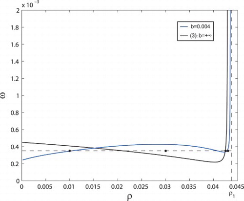
In Figure 1, two bifurcation curves are drawn for system (3(3) $\begin{array}{rl}\frac{\mathrm{d}x\left(t\right)}{\mathrm{d}t}& =\alpha x\left(t\right)(1-\beta x(t\left)\right)-x\left(t\right)y\left(t\right),\\ \frac{\mathrm{d}y\left(t\right)}{\mathrm{d}t}& ={\sigma }_1-{\delta }_{1}y\left(t\right)+\rho y\left(t\right)z\left(t\right),\\ \frac{\mathrm{d}z\left(t\right)}{\mathrm{d}t}& ={\sigma }_2-{\delta }_{2}z\left(t\right)+\omega x\left(t\right)z\left(t\right),\end{array}$(3) ) ($b=+\mathrm{\infty }$) and system (4(4) $\begin{array}{rl}\frac{\mathrm{d}x\left(t\right)}{\mathrm{d}t}& =\alpha x\left(t\right)(1-\beta x(t\left)\right)-x\left(t\right)y\left(t\right),\\ \frac{\mathrm{d}y\left(t\right)}{\mathrm{d}t}& ={\sigma }_1-{\delta }_{1}y\left(t\right)+\rho y\left(t\right)G\left(t\right),\\ \frac{\mathrm{d}z\left(t\right)}{\mathrm{d}t}& ={\sigma }_2-{\delta }_{2}z\left(t\right)+\omega x\left(t\right)z\left(t\right),\\ \frac{\mathrm{d}G\left(t\right)}{\mathrm{d}t}& =bz\left(t\right)-bG\left(t\right),\end{array}$(4) ) (b=0.004) in the same $\rho -\omega$ parameter plane. Both $E^{\ast }$ and $E^{+}$ are stable below the corresponding bifurcation curve and are unstable above the bifurcation curve. The bifurcation curves in Figure 1 are derived from equations $b_1(\rho ,\omega )b_2(\rho ,\omega )-b_3(\rho ,\omega )=0$ and $\left(B_1\right(\rho ,\omega \left)B_2\right(\rho ,\omega )-B_3(\rho ,\omega \left)\right)B_3(\rho ,\omega )-B_1^2(\rho ,\omega )B_4(\rho ,\omega )=0$, respectively. The shape of the bifurcation curve for system (3(3) $\begin{array}{rl}\frac{\mathrm{d}x\left(t\right)}{\mathrm{d}t}& =\alpha x\left(t\right)(1-\beta x(t\left)\right)-x\left(t\right)y\left(t\right),\\ \frac{\mathrm{d}y\left(t\right)}{\mathrm{d}t}& ={\sigma }_1-{\delta }_{1}y\left(t\right)+\rho y\left(t\right)z\left(t\right),\\ \frac{\mathrm{d}z\left(t\right)}{\mathrm{d}t}& ={\sigma }_2-{\delta }_{2}z\left(t\right)+\omega x\left(t\right)z\left(t\right),\end{array}$(3) ) is similar to the one in [7], which means that the simplified system (3(3) $\begin{array}{rl}\frac{\mathrm{d}x\left(t\right)}{\mathrm{d}t}& =\alpha x\left(t\right)(1-\beta x(t\left)\right)-x\left(t\right)y\left(t\right),\\ \frac{\mathrm{d}y\left(t\right)}{\mathrm{d}t}& ={\sigma }_1-{\delta }_{1}y\left(t\right)+\rho y\left(t\right)z\left(t\right),\\ \frac{\mathrm{d}z\left(t\right)}{\mathrm{d}t}& ={\sigma }_2-{\delta }_{2}z\left(t\right)+\omega x\left(t\right)z\left(t\right),\end{array}$(3) ) keeps the dynamics properties of the original model (1(1) $\begin{array}{rl}\frac{\mathrm{d}T\left(t\right)}{\mathrm{d}t}& =aT\left(t\right)(1-bT(t\left)\right)-nE\left(t\right)T\left(t\right),\\ \frac{\mathrm{d}E\left(t\right)}{\mathrm{d}t}& =s_1-d_{1}E\left(t\right)+k_{1}T\left(t\right)E\left(t\right)+pE\left(t\right)H\left(t\right),\\ \frac{\mathrm{d}H\left(t\right)}{\mathrm{d}t}& =s_2-d_{2}H\left(t\right)+k_{2}T\left(t\right)H\left(t\right),\end{array}$(1) ). When we consider a small b=0.004 for system (4(4) $\begin{array}{rl}\frac{\mathrm{d}x\left(t\right)}{\mathrm{d}t}& =\alpha x\left(t\right)(1-\beta x(t\left)\right)-x\left(t\right)y\left(t\right),\\ \frac{\mathrm{d}y\left(t\right)}{\mathrm{d}t}& ={\sigma }_1-{\delta }_{1}y\left(t\right)+\rho y\left(t\right)G\left(t\right),\\ \frac{\mathrm{d}z\left(t\right)}{\mathrm{d}t}& ={\sigma }_2-{\delta }_{2}z\left(t\right)+\omega x\left(t\right)z\left(t\right),\\ \frac{\mathrm{d}G\left(t\right)}{\mathrm{d}t}& =bz\left(t\right)-bG\left(t\right),\end{array}$(4) ), we found that the shape of the bifurcation curve has been changed. Correspondingly, the stable and unstable regions are also changed, which offers the possibility of stability switch due to the delay effect.

Figure 1. Stability regions of tumour-presence equilibria $E^{\ast }$ and $E^{+}$ and Hopf bifurcation are shown in the $\rho -\omega$ parameter plane.

In order to check the stability change, we choose four representative points in the $\rho -\omega$ plane in Figure 1. Here we fix $\omega =0.00035$ and vary ρ. If we choose $\rho =0.01$, there exist two tumour-presence equilibria, ${\tilde{E}}_1^{\ast }=(118.33,1.24882,27.9731),{\tilde{E}}_1^{+}=(118.33,1.24882,27.9731,27.9731).$ ${\tilde{E}}_1^{\ast }$ is stable (Figure 2a), but ${\tilde{E}}_1^{+}$ is unstable (Figure 2b).

Figure 2. The time evolution curves of system (3(3) $\begin{array}{rl}\frac{\mathrm{d}x\left(t\right)}{\mathrm{d}t}& =\alpha x\left(t\right)(1-\beta x(t\left)\right)-x\left(t\right)y\left(t\right),\\ \frac{\mathrm{d}y\left(t\right)}{\mathrm{d}t}& ={\sigma }_1-{\delta }_{1}y\left(t\right)+\rho y\left(t\right)z\left(t\right),\\ \frac{\mathrm{d}z\left(t\right)}{\mathrm{d}t}& ={\sigma }_2-{\delta }_{2}z\left(t\right)+\omega x\left(t\right)z\left(t\right),\end{array}$(3) ) (left panel) and system (4(4) $\begin{array}{rl}\frac{\mathrm{d}x\left(t\right)}{\mathrm{d}t}& =\alpha x\left(t\right)(1-\beta x(t\left)\right)-x\left(t\right)y\left(t\right),\\ \frac{\mathrm{d}y\left(t\right)}{\mathrm{d}t}& ={\sigma }_1-{\delta }_{1}y\left(t\right)+\rho y\left(t\right)G\left(t\right),\\ \frac{\mathrm{d}z\left(t\right)}{\mathrm{d}t}& ={\sigma }_2-{\delta }_{2}z\left(t\right)+\omega x\left(t\right)z\left(t\right),\\ \frac{\mathrm{d}G\left(t\right)}{\mathrm{d}t}& =bz\left(t\right)-bG\left(t\right),\end{array}$(4) ) (right panel). Here, we fix $\omega =0.00035$, b=0.004 and choose four different ρ as 0.01 (a and b), 0.03 (c and d), 0.0425 (e and f), 0.043 (g and h). (a) Local asymptotic stability of ${\tilde{E}}_1^{\ast }$. (b) The time evolution curves of system (4(4) $\begin{array}{rl}\frac{\mathrm{d}x\left(t\right)}{\mathrm{d}t}& =\alpha x\left(t\right)(1-\beta x(t\left)\right)-x\left(t\right)y\left(t\right),\\ \frac{\mathrm{d}y\left(t\right)}{\mathrm{d}t}& ={\sigma }_1-{\delta }_{1}y\left(t\right)+\rho y\left(t\right)G\left(t\right),\\ \frac{\mathrm{d}z\left(t\right)}{\mathrm{d}t}& ={\sigma }_2-{\delta }_{2}z\left(t\right)+\omega x\left(t\right)z\left(t\right),\\ \frac{\mathrm{d}G\left(t\right)}{\mathrm{d}t}& =bz\left(t\right)-bG\left(t\right),\end{array}$(4) ) around ${\tilde{E}}_1^{+}$ show periodic oscillations. (c) The time evolution curves of system (3(3) $\begin{array}{rl}\frac{\mathrm{d}x\left(t\right)}{\mathrm{d}t}& =\alpha x\left(t\right)(1-\beta x(t\left)\right)-x\left(t\right)y\left(t\right),\\ \frac{\mathrm{d}y\left(t\right)}{\mathrm{d}t}& ={\sigma }_1-{\delta }_{1}y\left(t\right)+\rho y\left(t\right)z\left(t\right),\\ \frac{\mathrm{d}z\left(t\right)}{\mathrm{d}t}& ={\sigma }_2-{\delta }_{2}z\left(t\right)+\omega x\left(t\right)z\left(t\right),\end{array}$(3) ) around ${\tilde{E}}_2^{\ast }$ show periodic oscillations. (d) Local asymptotic stability of ${\tilde{E}}_2^{+}$. (e) Local asymptotic stability of ${\tilde{E}}_3^{\ast }$. (f) The time evolution curves of system (4(4) $\begin{array}{rl}\frac{\mathrm{d}x\left(t\right)}{\mathrm{d}t}& =\alpha x\left(t\right)(1-\beta x(t\left)\right)-x\left(t\right)y\left(t\right),\\ \frac{\mathrm{d}y\left(t\right)}{\mathrm{d}t}& ={\sigma }_1-{\delta }_{1}y\left(t\right)+\rho y\left(t\right)G\left(t\right),\\ \frac{\mathrm{d}z\left(t\right)}{\mathrm{d}t}& ={\sigma }_2-{\delta }_{2}z\left(t\right)+\omega x\left(t\right)z\left(t\right),\\ \frac{\mathrm{d}G\left(t\right)}{\mathrm{d}t}& =bz\left(t\right)-bG\left(t\right),\end{array}$(4) ) around ${\tilde{E}}_3^{+}$ show periodic oscillations. (g ) Local asymptotic stability of ${\tilde{E}}_4^{\ast }$. (h) Local asymptotic stability of ${\tilde{E}}_4^{+}$.

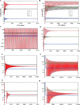
If we choose $\rho =0.03$, there exist two tumour-presence equilibria, ${\tilde{E}}_2^{\ast }=(46.615,1.48348,9.82299),{\tilde{E}}_2^{+}=(46.615,1.48348,9.82299,9.82299).$ ${\tilde{E}}_2^{\ast }$ is unstable (Figure 2c), but ${\tilde{E}}_2^{+}$ is stable (Figure 2d).

If we choose $\rho =0.0425$, there exist two tumour-presence equilibria, ${\tilde{E}}_3^{\ast }=(4.10569,1.62257,7.09445),{\tilde{E}}_3^{+}=(4.10569,1.62257,7.09445,7.09445).$ ${\tilde{E}}_3^{\ast }$ is stable (Figure 2e), but ${\tilde{E}}_3^{+}$ is unstable (Figure 2f).

If we choose $\rho =0.043$, there exist two tumour-presence equilibria, ${\tilde{E}}_4^{\ast }=(2.43096,1.62805,7.01765),{\tilde{E}}_4^{+}=(2.43096,1.62805,7.01765,7.01765).$ ${\tilde{E}}_4^{\ast }$ is stable (Figure 2g), and ${\tilde{E}}_4^{+}$ is stable (Figure 2h).

Next, we check the coefficients of $Q\left(b\right)$ to verify Theorem 2.5 by finding different values of ρ and ω under condition (7(7) $\begin{array}{rl}{b}_1{b}_2-b_3& =\left(\alpha \beta x^{\ast }+\frac{{\sigma }_1}{y^{\ast }}\right)\left(\alpha \beta x^{\ast }\frac{{\sigma }_1}{y^{\ast }}+\alpha \beta x^{\ast }\frac{{\sigma }_2}{z^{\ast }}+\frac{{\sigma }_1}{y^{\ast }}\frac{{\sigma }_2}{z^{\ast }}\right)\\ & +\frac{{\sigma }_2}{z^{\ast }}\left(\alpha \beta x^{\ast }\frac{{\sigma }_2}{z^{\ast }}+\frac{{\sigma }_1}{y^{\ast }}\frac{{\sigma }_2}{z^{\ast }}\right)-\rho \omega x^{\ast }{y}^{\ast }{z}^{\ast }>0,\end{array}$(7) ). It means that we should look for such point $(\rho ,\omega )$ under the bifurcation curve (b=0) in Figure 1. For system (3(3) $\begin{array}{rl}\frac{\mathrm{d}x\left(t\right)}{\mathrm{d}t}& =\alpha x\left(t\right)(1-\beta x(t\left)\right)-x\left(t\right)y\left(t\right),\\ \frac{\mathrm{d}y\left(t\right)}{\mathrm{d}t}& ={\sigma }_1-{\delta }_{1}y\left(t\right)+\rho y\left(t\right)z\left(t\right),\\ \frac{\mathrm{d}z\left(t\right)}{\mathrm{d}t}& ={\sigma }_2-{\delta }_{2}z\left(t\right)+\omega x\left(t\right)z\left(t\right),\end{array}$(3) ) without time delay, the tumour-presence equilibrium is locally asymptotically stable.

If we choose $(\rho ,\omega )=(0.0436,0.00035)$, then $b_1{b}_2-b_3=4.5314\times {10}^{-4}>0$. We have $P_0=2.89088\times {10}^{-9}>0,P_1=9.70195\times {10}^{-7}>0,P_2=4.88179\times {10}^{-5}>0,P_3=4.5314\times {10}^{-4}>0$ satisfy Case (I), where we have no chance to have stability change. So, we have $Q\left(b\right)>0$ (see Figure 3, Case (I)), which ensures that $E^{+}$ is always locally asymptotically stable.

Figure 3. The curves of $Q\left(b\right)$ with respect to b. Case (I): we choose $(\rho ,\omega )=(0.0436,0.00035)$, and we have $Q\left(b\right)>0$ when b>0. Case (II): we choose $(\rho ,\omega )=(0.043,0.0001)$, and we have $Q\left(b\right)>0$ when b>0. Case (III): we choose $(\rho ,\omega )=(0.043,0.00035)$, and we have $Q\left(b\right)>0$ when $0<b<\underset{\_}{b}=0.00433351$ or $b>\overline{b}=0.219156$.

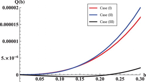
If we choose $(\rho ,\omega )=(0.043,0.0001)$, then $b_1{b}_2-b_3=6.12286\times {10}^{-4}>0$. We have $P_0=9.0695\times {10}^{-8}>0,P_1=-1.29001\times {10}^{-6}<0,P_2=3.94716\times {10}^{-5}>0,P_3=6.12286\times {10}^{-4}>0$ satisfy Case (II). By calculations, we have $b^{\ast }=0.0126295<0.0701071=M$ and $Q\left(b^{\ast }\right)=8.19322\times {10}^{-8}>0$ which are not satisfied with condition (9(9) $b^{\ast }=\frac{-P_2+\sqrt{P_2^2-3P_1{P}_3}}{3P_3}>\frac{9P_0{P}_3-P_1{P}_2}{2P_2^2-6P_1{P}_3}\equiv M.$(9) ). So, we have $Q\left(b\right)>0$ (see Figure 3, Case (II)), which ensures that $E^{+}$ is always locally asymptotically stable.

If we choose $(\rho ,\omega )=(0.043,0.00035)$, then $b_1{b}_2-b_3=2.15328\times {10}^{-4}>0$. We have $P_0=1.97876\times {10}^{-8}>0,P_1=-4.45197\times {10}^{-6}<0,P_2=-2.72882\times {10}^{-5}<0,P_3=2.15328\times {10}^{-4}>0$ satisfy Case (III). By calculations, we have $b^{\ast }=0.135389>-0.0114816=M$ and $Q\left(b^{\ast }\right)=-5.48778\times {10}^{-7}<0$ which are satisfied with condition (9(9) $b^{\ast }=\frac{-P_2+\sqrt{P_2^2-3P_1{P}_3}}{3P_3}>\frac{9P_0{P}_3-P_1{P}_2}{2P_2^2-6P_1{P}_3}\equiv M.$(9) ). There exist $\underset{\_}{b}=0.00433351$ and $\overline{b}=0.219156$ (see Figure 3, Case (III)), which ensures that $E^{+}$ is locally asymptotically stable for $0<b<\underset{\_}{b}$ or $b>\overline{b}$ and unstable for $\underset{\_}{b}<b<\overline{b}$.

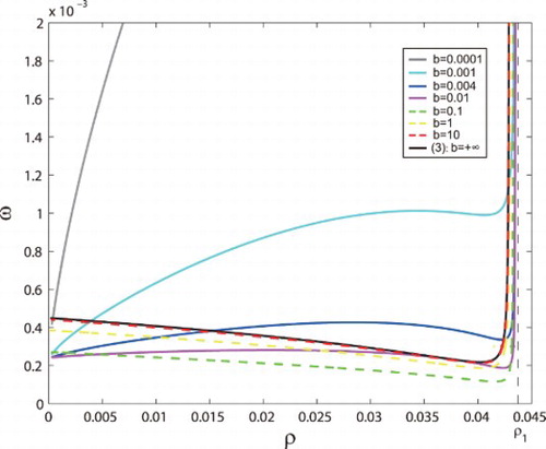
Figure 4 shows the change of the bifurcation curve as the parameter b varies. The bifurcation curves ($b\ne 0$) are satisfied with $Q(\rho ,\omega )=0$ for each fixed b. $b=0.0001,0.001,0.004,0.01,0.1,1$ and 10 are corresponding to system (4(4) $\begin{array}{rl}\frac{\mathrm{d}x\left(t\right)}{\mathrm{d}t}& =\alpha x\left(t\right)(1-\beta x(t\left)\right)-x\left(t\right)y\left(t\right),\\ \frac{\mathrm{d}y\left(t\right)}{\mathrm{d}t}& ={\sigma }_1-{\delta }_{1}y\left(t\right)+\rho y\left(t\right)G\left(t\right),\\ \frac{\mathrm{d}z\left(t\right)}{\mathrm{d}t}& ={\sigma }_2-{\delta }_{2}z\left(t\right)+\omega x\left(t\right)z\left(t\right),\\ \frac{\mathrm{d}G\left(t\right)}{\mathrm{d}t}& =bz\left(t\right)-bG\left(t\right),\end{array}$(4) ), while $b=+\mathrm{\infty }$ is corresponding to system (3(3) $\begin{array}{rl}\frac{\mathrm{d}x\left(t\right)}{\mathrm{d}t}& =\alpha x\left(t\right)(1-\beta x(t\left)\right)-x\left(t\right)y\left(t\right),\\ \frac{\mathrm{d}y\left(t\right)}{\mathrm{d}t}& ={\sigma }_1-{\delta }_{1}y\left(t\right)+\rho y\left(t\right)z\left(t\right),\\ \frac{\mathrm{d}z\left(t\right)}{\mathrm{d}t}& ={\sigma }_2-{\delta }_{2}z\left(t\right)+\omega x\left(t\right)z\left(t\right),\end{array}$(3) ). Firstly, stability regions become smaller, and then become larger with increasing b. Finally, the bifurcation curve of system (4(4) $\begin{array}{rl}\frac{\mathrm{d}x\left(t\right)}{\mathrm{d}t}& =\alpha x\left(t\right)(1-\beta x(t\left)\right)-x\left(t\right)y\left(t\right),\\ \frac{\mathrm{d}y\left(t\right)}{\mathrm{d}t}& ={\sigma }_1-{\delta }_{1}y\left(t\right)+\rho y\left(t\right)G\left(t\right),\\ \frac{\mathrm{d}z\left(t\right)}{\mathrm{d}t}& ={\sigma }_2-{\delta }_{2}z\left(t\right)+\omega x\left(t\right)z\left(t\right),\\ \frac{\mathrm{d}G\left(t\right)}{\mathrm{d}t}& =bz\left(t\right)-bG\left(t\right),\end{array}$(4) ) will tend to the bifurcation curve of system (3(3) $\begin{array}{rl}\frac{\mathrm{d}x\left(t\right)}{\mathrm{d}t}& =\alpha x\left(t\right)(1-\beta x(t\left)\right)-x\left(t\right)y\left(t\right),\\ \frac{\mathrm{d}y\left(t\right)}{\mathrm{d}t}& ={\sigma }_1-{\delta }_{1}y\left(t\right)+\rho y\left(t\right)z\left(t\right),\\ \frac{\mathrm{d}z\left(t\right)}{\mathrm{d}t}& ={\sigma }_2-{\delta }_{2}z\left(t\right)+\omega x\left(t\right)z\left(t\right),\end{array}$(3) ) as b tends to infinity.

Figure 4. Hopf bifurcation curves of $E^{+}$ are shown in the $\rho -\omega$ parameter plane for a different b.

4. Conclusion and discussion

In this paper, first, we reduced the previous system in [7] by ignoring a weak direct immune activation by the TCs. We found that the simplified three-dimensional system (3(3) $\begin{array}{rl}\frac{\mathrm{d}x\left(t\right)}{\mathrm{d}t}& =\alpha x\left(t\right)(1-\beta x(t\left)\right)-x\left(t\right)y\left(t\right),\\ \frac{\mathrm{d}y\left(t\right)}{\mathrm{d}t}& ={\sigma }_1-{\delta }_{1}y\left(t\right)+\rho y\left(t\right)z\left(t\right),\\ \frac{\mathrm{d}z\left(t\right)}{\mathrm{d}t}& ={\sigma }_2-{\delta }_{2}z\left(t\right)+\omega x\left(t\right)z\left(t\right),\end{array}$(3) ) can keep the intrinsic dynamics properties of the original model (1(1) $\begin{array}{rl}\frac{\mathrm{d}T\left(t\right)}{\mathrm{d}t}& =aT\left(t\right)(1-bT(t\left)\right)-nE\left(t\right)T\left(t\right),\\ \frac{\mathrm{d}E\left(t\right)}{\mathrm{d}t}& =s_1-d_{1}E\left(t\right)+k_{1}T\left(t\right)E\left(t\right)+pE\left(t\right)H\left(t\right),\\ \frac{\mathrm{d}H\left(t\right)}{\mathrm{d}t}& =s_2-d_{2}H\left(t\right)+k_{2}T\left(t\right)H\left(t\right),\end{array}$(1) ) due to the similar expression (7(7) $\begin{array}{rl}{b}_1{b}_2-b_3& =\left(\alpha \beta x^{\ast }+\frac{{\sigma }_1}{y^{\ast }}\right)\left(\alpha \beta x^{\ast }\frac{{\sigma }_1}{y^{\ast }}+\alpha \beta x^{\ast }\frac{{\sigma }_2}{z^{\ast }}+\frac{{\sigma }_1}{y^{\ast }}\frac{{\sigma }_2}{z^{\ast }}\right)\\ & +\frac{{\sigma }_2}{z^{\ast }}\left(\alpha \beta x^{\ast }\frac{{\sigma }_2}{z^{\ast }}+\frac{{\sigma }_1}{y^{\ast }}\frac{{\sigma }_2}{z^{\ast }}\right)-\rho \omega x^{\ast }{y}^{\ast }{z}^{\ast }>0,\end{array}$(7) ) and the shape of the bifurcation curve (see Figure 1). Second, we incorporated the time delay into the ODE model to modelling the lag of the activation of ECs from HTCs. If we directly incorporate the delay term, it is difficult to calculate the transcendent characteristic equation. Alternatively, we used a function $G\left(t\right)={\int }_0^{\mathrm{\infty }}b{e}^{-bu}z(t-u)\mathrm{d}u$ to model this immune activation delay effect at the cost of increasing one dimension. The immune activation depends on the density of HTCs at the present time t when b is large representing a weak delay effect, on the other hand, the activation depends on the density of HTCs at the past time t−u when b is small indicating a strong delay effect.

Next, we explained the biological meanings of two critical thresholds of ρ (i.e., ${\rho }_1$ and ${\rho }_0$). Note that ρ is the scaled parameter of p which is the activation rate of ECs by HTCs. For system (4(4) $\begin{array}{rl}\frac{\mathrm{d}x\left(t\right)}{\mathrm{d}t}& =\alpha x\left(t\right)(1-\beta x(t\left)\right)-x\left(t\right)y\left(t\right),\\ \frac{\mathrm{d}y\left(t\right)}{\mathrm{d}t}& ={\sigma }_1-{\delta }_{1}y\left(t\right)+\rho y\left(t\right)G\left(t\right),\\ \frac{\mathrm{d}z\left(t\right)}{\mathrm{d}t}& ={\sigma }_2-{\delta }_{2}z\left(t\right)+\omega x\left(t\right)z\left(t\right),\\ \frac{\mathrm{d}G\left(t\right)}{\mathrm{d}t}& =bz\left(t\right)-bG\left(t\right),\end{array}$(4) ), to make sure the tumour-free equilibrium $E^{-}=(x^{-},y^{-},z^{-},G^{-})=(0,{\sigma }_1{\delta }_2/({\delta }_1{\delta }_2-\rho {\sigma }_2),{\sigma }_2/{\delta }_2,{\sigma }_2/{\delta }_2)$ to be existing, we need the condition $\rho <{\delta }_1{\delta }_2/{\sigma }_2$, and we define ${\rho }_0\equiv {\delta }_1{\delta }_2/{\sigma }_2$, that is $\rho <{\rho }_0$. Similarly, to ensure the tumour-presence equilibrium $E^{+}=(x^{+},y^{+},z^{+},G^{+})=(x^{\ast },y^{\ast },z^{\ast },z^{\ast })$ to be existing, we need the condition $\rho <{\delta }_1{\delta }_2/{\sigma }_2-{\sigma }_1{\delta }_2/\alpha {\sigma }_2$, and we define ${\rho }_1\equiv {\delta }_1{\delta }_2/{\sigma }_2-{\sigma }_1{\delta }_2/\alpha {\sigma }_2$, that is $\rho <{\rho }_1$. In short, $\rho <{\rho }_0$ and $\rho <{\rho }_1$ are conditions for the existences of $E^{-}$ and $E^{+}$, respectively. From the biological view, if the activation rate of ECs by HTCs is more than ${\rho }_1$, the tumour-presence equilibrium $E^{+}$ will disappear, that is TCs can be eradicated from the patient's body. Further, if the activation rate of ECs by HTCs is more than ${\rho }_0$, the tumour-free equilibrium $E^{-}$ will also vanish. It means that overactive immune response can destroy the normal cells. It is in line with that an immune system is crucial but too strong immune response is harmful. In other words, an appropriate immune response is good in the control of tumour growth (i.e., ${\rho }_1<\rho <{\rho }_0$). As we can see that the Hopf bifurcation curves of $E^{+}$ can never exceed the vertical line $\rho ={\rho }_1$ in the $\rho -\omega$ parameter plane in Figure 4.

Compared with system (3(3) $\begin{array}{rl}\frac{\mathrm{d}x\left(t\right)}{\mathrm{d}t}& =\alpha x\left(t\right)(1-\beta x(t\left)\right)-x\left(t\right)y\left(t\right),\\ \frac{\mathrm{d}y\left(t\right)}{\mathrm{d}t}& ={\sigma }_1-{\delta }_{1}y\left(t\right)+\rho y\left(t\right)z\left(t\right),\\ \frac{\mathrm{d}z\left(t\right)}{\mathrm{d}t}& ={\sigma }_2-{\delta }_{2}z\left(t\right)+\omega x\left(t\right)z\left(t\right),\end{array}$(3) ), the introduction of new parameter b>0 in system (4(4) $\begin{array}{rl}\frac{\mathrm{d}x\left(t\right)}{\mathrm{d}t}& =\alpha x\left(t\right)(1-\beta x(t\left)\right)-x\left(t\right)y\left(t\right),\\ \frac{\mathrm{d}y\left(t\right)}{\mathrm{d}t}& ={\sigma }_1-{\delta }_{1}y\left(t\right)+\rho y\left(t\right)G\left(t\right),\\ \frac{\mathrm{d}z\left(t\right)}{\mathrm{d}t}& ={\sigma }_2-{\delta }_{2}z\left(t\right)+\omega x\left(t\right)z\left(t\right),\\ \frac{\mathrm{d}G\left(t\right)}{\mathrm{d}t}& =bz\left(t\right)-bG\left(t\right),\end{array}$(4) ) did not change the values of tumour-free and tumour-presence equilibria; however, it can substantially change the dynamics properties. Specifically, the delay can lead to stability changes exhibiting destabilization as well as stabilization of the tumour-presence equilibrium, which plays a dual role. We provided some numerical simulations to show that dynamics can be changed at the branch of the tumour-presence equilibria $E^{\ast }$ and $E^{+}$, resulting in Hopf bifurcation. In Figure 1, both $E^{\ast }$ and $E^{+}$ are stable below the corresponding bifurcation curve and are unstable above the bifurcation curve. To show the possible stability change of $E^{\ast }$ and $E^{+}$, we chose four points $(0.01,0.00035),(0.03,0.00035),(0.0425,0.00035)$ and $(0.043,0.00035)$ in the $\rho -\omega$ plane. By comparing the left panel for system (3(3) $\begin{array}{rl}\frac{\mathrm{d}x\left(t\right)}{\mathrm{d}t}& =\alpha x\left(t\right)(1-\beta x(t\left)\right)-x\left(t\right)y\left(t\right),\\ \frac{\mathrm{d}y\left(t\right)}{\mathrm{d}t}& ={\sigma }_1-{\delta }_{1}y\left(t\right)+\rho y\left(t\right)z\left(t\right),\\ \frac{\mathrm{d}z\left(t\right)}{\mathrm{d}t}& ={\sigma }_2-{\delta }_{2}z\left(t\right)+\omega x\left(t\right)z\left(t\right),\end{array}$(3) ) and the right panel for system (4(4) $\begin{array}{rl}\frac{\mathrm{d}x\left(t\right)}{\mathrm{d}t}& =\alpha x\left(t\right)(1-\beta x(t\left)\right)-x\left(t\right)y\left(t\right),\\ \frac{\mathrm{d}y\left(t\right)}{\mathrm{d}t}& ={\sigma }_1-{\delta }_{1}y\left(t\right)+\rho y\left(t\right)G\left(t\right),\\ \frac{\mathrm{d}z\left(t\right)}{\mathrm{d}t}& ={\sigma }_2-{\delta }_{2}z\left(t\right)+\omega x\left(t\right)z\left(t\right),\\ \frac{\mathrm{d}G\left(t\right)}{\mathrm{d}t}& =bz\left(t\right)-bG\left(t\right),\end{array}$(4) ) in Figure 2, we found that the introduction of time delay indeed caused the dynamics change.

The bifurcation curves ($b\ne 0$) are satisfied with $Q(\rho ,\omega )=0$ for each fixed b. When we consider a very small b (i.e., a strong delay effect, that is, the activation of ECs by HTCs is very slow), the stable region can be very large. And the stable region will tend to infinite as b tends to 0 (see the grey curve b=0.0001, cyan curve b=0.001, blue curve b=0.004 and magenta curve b=0.01 in Figure 4). As a consequence, the tumour-presence equilibrium is always stable and dominant under the condition $b_1{b}_2-b_3>0$ ensured by Proposition 2.6, which means that TCs cannot be eradicated from the body. When we further increase b, the bifurcation curve will go down and the stability region in the $\rho -\omega$ plane will become smaller. But the bifurcation curve can never reach the ρ axis, because when ω is small, the stability region always exists regardless of any changes of ρ and b. There must exist a critical value $\hat{b}$, which makes the stability region to be minimal. When we increase b to exceed this $\hat{b}$, the bifurcation curve of system (4(4) $\begin{array}{rl}\frac{\mathrm{d}x\left(t\right)}{\mathrm{d}t}& =\alpha x\left(t\right)(1-\beta x(t\left)\right)-x\left(t\right)y\left(t\right),\\ \frac{\mathrm{d}y\left(t\right)}{\mathrm{d}t}& ={\sigma }_1-{\delta }_{1}y\left(t\right)+\rho y\left(t\right)G\left(t\right),\\ \frac{\mathrm{d}z\left(t\right)}{\mathrm{d}t}& ={\sigma }_2-{\delta }_{2}z\left(t\right)+\omega x\left(t\right)z\left(t\right),\\ \frac{\mathrm{d}G\left(t\right)}{\mathrm{d}t}& =bz\left(t\right)-bG\left(t\right),\end{array}$(4) ) will go up and stability regions will become larger (see the green dashed curve b=0.1, yellow dashed curve b=1 and red dashed curve b=10 in Figure 4). Finally, the bifurcation curve of system (4(4) $\begin{array}{rl}\frac{\mathrm{d}x\left(t\right)}{\mathrm{d}t}& =\alpha x\left(t\right)(1-\beta x(t\left)\right)-x\left(t\right)y\left(t\right),\\ \frac{\mathrm{d}y\left(t\right)}{\mathrm{d}t}& ={\sigma }_1-{\delta }_{1}y\left(t\right)+\rho y\left(t\right)G\left(t\right),\\ \frac{\mathrm{d}z\left(t\right)}{\mathrm{d}t}& ={\sigma }_2-{\delta }_{2}z\left(t\right)+\omega x\left(t\right)z\left(t\right),\\ \frac{\mathrm{d}G\left(t\right)}{\mathrm{d}t}& =bz\left(t\right)-bG\left(t\right),\end{array}$(4) ) will tend to the bifurcation curve of system (3(3) $\begin{array}{rl}\frac{\mathrm{d}x\left(t\right)}{\mathrm{d}t}& =\alpha x\left(t\right)(1-\beta x(t\left)\right)-x\left(t\right)y\left(t\right),\\ \frac{\mathrm{d}y\left(t\right)}{\mathrm{d}t}& ={\sigma }_1-{\delta }_{1}y\left(t\right)+\rho y\left(t\right)z\left(t\right),\\ \frac{\mathrm{d}z\left(t\right)}{\mathrm{d}t}& ={\sigma }_2-{\delta }_{2}z\left(t\right)+\omega x\left(t\right)z\left(t\right),\end{array}$(3) ) as b tends to infinity (see the red dashed curve b=10 and the black curve $b=+\mathrm{\infty }$ of system (3(3) $\begin{array}{rl}\frac{\mathrm{d}x\left(t\right)}{\mathrm{d}t}& =\alpha x\left(t\right)(1-\beta x(t\left)\right)-x\left(t\right)y\left(t\right),\\ \frac{\mathrm{d}y\left(t\right)}{\mathrm{d}t}& ={\sigma }_1-{\delta }_{1}y\left(t\right)+\rho y\left(t\right)z\left(t\right),\\ \frac{\mathrm{d}z\left(t\right)}{\mathrm{d}t}& ={\sigma }_2-{\delta }_{2}z\left(t\right)+\omega x\left(t\right)z\left(t\right),\end{array}$(3) )). In other words, the decrease of delay will decrease first and then increase the stability region. In a word, a critical time delay exists and makes the stable region of tumour-presence equilibrium consisting of $Q\left(\hat{b}\right)=0$ and axes to be minimal. This means that an appropriate immune activation time delay $\hat{b}$ can minimally control the tumour growth.

In system (4(4) $\begin{array}{rl}\frac{\mathrm{d}x\left(t\right)}{\mathrm{d}t}& =\alpha x\left(t\right)(1-\beta x(t\left)\right)-x\left(t\right)y\left(t\right),\\ \frac{\mathrm{d}y\left(t\right)}{\mathrm{d}t}& ={\sigma }_1-{\delta }_{1}y\left(t\right)+\rho y\left(t\right)G\left(t\right),\\ \frac{\mathrm{d}z\left(t\right)}{\mathrm{d}t}& ={\sigma }_2-{\delta }_{2}z\left(t\right)+\omega x\left(t\right)z\left(t\right),\\ \frac{\mathrm{d}G\left(t\right)}{\mathrm{d}t}& =bz\left(t\right)-bG\left(t\right),\end{array}$(4) ), we have introduced a delay effect by a weak kernel, i.e., $F\left(u\right)=b{e}^{-bu}$(b>0). For the further study, we can introduce a delay effect by a non-monotone kernel, i.e., $F\left(u\right)=b^{2}u{e}^{-bu}$(b>0).

Acknowledgements

The authors thank the editor and two anonymous reviewers for their constructive comments that improved the manuscript.

Disclosure statement

No potential conflict of interest was reported by the authors.

Additional information

Funding

This research was supported by Grants-in-Aid Scientific Research (C) No. 26400211, Japan Society for Promotion of Science.

References

- J. Arciero, T. Jackson, and D. Kirscher, A mathematical model of tumor–immune evasion and siRNA treatment, Discrete Contin. Dyn. Syst. Ser. B 4 (2004), pp. 39–58.
- P. Bi and S. Ruan, Bifurcations in delay differential equations and applications to tumor and immune system interaction models, SIAM J. Appl. Dyn. Syst. 12 (2013), pp. 1847–1888. doi: 10.1137/120887898
- L.G. de Pillis, W. Gu, and A.E. Radunskaya, Mixed immunotherapy and chemotherapy of tumors: modeling, application and biological interpretations, J. Theor. Biol. 238 (2006), pp. 841–862. doi: 10.1016/j.jtbi.2005.06.037
- L.G. de Pillis, A.E. Radunskaya, and C.L. Wiseman, A validated mathematical model of cell-mediated immune response to tumor growth, Cancer Res. 65 (2005), pp. 7950–7958.
- K.E. de Visser, A. Eichten, and L.M. Coussens, Paradoxical roles of the immune system during cancer development, Nat. Rev. Cancer 6 (2006), pp. 24–37. doi: 10.1038/nrc1782
- Y. Dong, H. Gang, R. Miyazaki, and Y. Takeuchi, Dynamics in a tumor immune system with time delays, Appl. Math. Comput. 252 (2015), pp. 99–113.
- Y. Dong, R. Miyazaki, and Y. Takeuchi, Mathematical modeling on helper T cells in a tumor immune system, Discrete Contin. Dyn. Syst. Ser. B 19 (2014), pp. 55–72. doi: 10.3934/dcdsb.2014.19.55
- A. d'Onofrio, A general framework for modeling tumor–immune system competition and immunotherapy: Mathematical analysis and biomedical inferences, Physica D 208 (2005), pp. 220–235. doi: 10.1016/j.physd.2005.06.032
- A. d'Onofrio, Tumor evasion from immune system control: Strategies of a MISS to become a MASS, Chaos, Solitons and Fractals 31 (2007), pp. 261–268. doi: 10.1016/j.chaos.2005.10.006
- A. d'Onofrio, Metamodeling tumor–immune system interaction, tumor evasion and immunotherapy, Math. Comput. Model. 47 (2008), pp. 614–637. doi: 10.1016/j.mcm.2007.02.032
- A. d'Onofrio, F. Gatti, P. Cerrai, and L. Freschi, Delay-induced oscillatory dynamics of tumor–immune system interaction, Math. Comput. Model. 51 (2010), pp. 572–591. doi: 10.1016/j.mcm.2009.11.005
- G.B. Ermentrout, Simulating, Analyzing, and Animating Dynamical Systems: A Guide to XPPAUT for Researchers and Students, SIAM, Philadelphia, 2002.
- M. Galach, Dynamics of the tumor–immune system competition: The effect of time delay, Int. J. Appl. Math. Comput. Sci. 13 (2003), pp. 395–406.
- I. Kareva, F. Berezovskaya, and C. Castillo-Chavez, Myeloid cells in tumour–immune interactions, J. Biol. Dynam. 4 (2010), pp. 315–327. doi: 10.1080/17513750903261281
- D. Kirschner and J. Panetta, Modeling immunotherapy of the tumor–immune interaction, J. Math. Biol. 37 (1998), pp. 235–252. doi: 10.1007/s002850050127
- V. Kuznetsov, I. Makalkin, M. Taylor, and A. Perelson, Nonlinear dynamics of immunogenic tumors: Parameter estimation and global bifurcation analysis, Bull. Math. Biol. 2 (1994), pp. 295–321. doi: 10.1007/BF02460644
- O. Lejeune, M. Chaplain, and I. Akili, Oscillations and bistability in the dynamics of cytotoxic reactions mediated by the response of immune cells to solid tumors, Math. Comput. Model. 47 (2008), pp. 649–662. doi: 10.1016/j.mcm.2007.02.026
- D. Liu, S. Ruan, and D. Zhu, Stable periodic oscillations in a two-stage cancer model of tumor and immune system interactions, Math. Biosci. Eng. 9 (2012), pp. 347–368. doi: 10.3934/mbe.2012.9.785
- F.A. Rihan, D.H.A. Rahmana, S. Lakshmanana, and A.S. Alkhajeh, A time delay model of tumour–immune system interactions: Global dynamics, parameter estimation, sensitivity analysis, Appl. Math. Comput. 232 (2014), pp. 606–623.
- M. Saleem, T. Agrawal, and A. Anees, A study of tumour growth based on stoichiometric principles: A continuous model and its discrete analogue, J. Biol. Dynam. 8 (2014), pp. 117–134. doi: 10.1080/17513758.2014.913718