Disease dynamics in a coupled cholera model linking within-host and between-host interactions

ABSTRACT

A new modelling framework is proposed to study the within-host and between-host dynamics of cholera, a severe intestinal infection caused by the bacterium Vibrio cholerae. The within-host dynamics are characterized by the growth of highly infectious vibrios inside the human body. These vibrios shed from humans contribute to the environmental bacterial growth and the transmission of the disease among humans, providing a link from the within-host dynamics at the individual level to the between-host dynamics at the population and environmental level. A fast-slow analysis is conducted based on the two different time scales in our model. In particular, a bifurcation study is performed, and sufficient and necessary conditions are derived that lead to a backward bifurcation in cholera epidemics. Our result regarding the backward bifurcation highlights the challenges in the prevention and control of cholera.

KEYWORDS:

• Cholera coupled models
• within-host and between-host dynamics
• fast-slow analysis
• backward bifurcation
• local and global stability
• type reproduction number

AMS SUBJECT CLASSIFICATION:

• 47H20
• 34D20
• 37H20

1. Introduction

Mathematical modelling of infectious diseases has played a significant role in furthering our understanding of disease dynamics and developing effective prevention and control measures against epidemics. For infectious diseases, there are two typical modelling approaches to study the disease infection, and they are usually considered separately. One is to use epidemiological models to investigate disease transmission on a population level [1], which concerns the between-host dynamics of the diseases. The other is to use immunological models to study the disease at the individual level, which is focused on the within-host dynamics. To link these dynamical processes at different levels, coupled (or nested) modelling approach is employed, and indeed this approach can offer new insight into the host–pathogen interactions (see [3,20] and references therein). The within- and between-host dynamics have been studied for several infectious diseases using the nested models (e.g. [7,9,11–16,25]). However, to the best of our knowledge, no existing work has attempted to address the coupled within- and between-host dynamics of cholera (a severe water-borne gastroenteric disease caused by the bacterium Vibrio cholerae), despite the fact that a large body of work has been devoted to its population level modelling (e.g. [4–6,17,21,22,26,28,29,32–36]). It is also worth mentioning that some of these between-host models have incorporated both human and environmental transmission pathways with nonlinear disease incidence functions (see, e.g. [10,26,27,28,31] and the references therein).

When vibrios from the contaminated environment (typically, water) are ingested by a person and reach the small intestine, complex biological, chemical and genomic interactions occur that lead to human cholera, whose pathogenicity and aetiology remain a very active research area [8]. Generally speaking, the environmental vibrios undergo evolutions through horizontal gene transfer and the formation of a toxin complex. As a result, highly toxic and infectious vibrios are generated with a large inoculum size, which cause severe diarrhea and are subsequently excreted out of the human body through shedding. Clinical studies [23] have found that these freshly shed vibrios are up to 700-fold in terms of infectivity compared to environmental vibrios, and they remain at this highly infectious state out of the human body for several hours during which time they can be transmitted through person-to-person contacts (e.g. by shaking hands, or consuming foods prepared by household people with dirty/contaminated hands). Unfortunately, our knowledge of the precise mechanisms of the bacterial growth and evolution inside the human body and their impact on cholera epidemics at the population level, and the quantification of such mechanisms towards the design of effective disease control and prevention strategies, remains limited at present.

The goal of this work is to fill in our knowledge gap through mathematical modelling and analysis, as a first attempt, in that direction. A multi-scale model is formulated in this paper that couples the within-host and between-host dynamics of cholera. Essentially, we quantitatively distinguish the two types of vibrios: the environmental vibrios which have relatively low infectivity, and the human vibrios (which are formed within human body and then shed out into the environment) that are highly infectious. The highly infectious vibrios live only for a short period of time (in hours) compared to that of the environmental vibrios (in months), but they directly determine the transmission rate through person-to-person contacts and largely contribute to the growth of the vibrios in the aquatic environment. We note that a standard assumption in almost all the afore-mentioned mathematical cholera studies is that the persistence of environmental vibrios and the disease spread among human populations are independent of within-host disease dynamics, which leads to relatively simple, usually constant, formulations in terms of the associated per capita rates of interactions. In contrast, our modelling framework incorporates a general representation of the incidence and the bacterial growth and persistence, and explicitly link disease dynamics at the population and individual levels through the concept of human vibrios. Our approach is different from traditional coupling principles [14] employed in nested models. Specifically, our explicit linkage is achieved by postulating the interaction between the cholera strains in the environment and those inside human hosts, instead of the cell–pathogen immunological interaction within a single host.

We shall mention that in the work of Hartley et al. [17], the authors also classified the vibrios into two types: lower infective and hyper infective. However, there are important differences between these two studies. First, their classification is only concerned with environmental vibrios and there are no within-host dynamics in their work. Second, our model has incorporated both indirect transmission and direct transmission pathways, while the work in [17] only has the indirect transmission route. Third, all the transmission rates in [17] are constant whereas our model utilizes variable transmission rates, dependent on both the environmental and human vibrios, to explicitly link the fast and slow dynamics. Additionally, their cholera study has a major focus on the medical aspects, whereas our work is more mathematically sophisticated.

The remainder of the paper is organized as follows. Section 2 presents the formulation of the cholera model linking the within-host and between-host dynamics. In Section 3, we analyse the coupled model by using the fast-slow analysis, utilizing the time scale separation for the dynamical processes associated with the individual host and the environment and human population. Global dynamics of the subsystems (i.e. the slow and fast systems) are studied separately. For the slow system, we calculate the corresponding type reproduction number of the infectious humans, and use it to investigate the disease threshold dynamics and analyse the local and global stabilities of the equilibrium solutions. One of our main findings is that our model exhibits a backward bifurcation, which has never been reported in previous cholera studies. A precise condition under which the backward bifurcation occurs in the slow system is obtained. For the fast system, the global stability of the unique equilibrium is established. In addition, we present numerical simulation results to verify our analysis, particularly for the coupled system dynamics. Finally, we wrap up the paper with conclusions and discussion in Section 4.

2. Model formulation

Cholera infection involves different time scales. The between-host and environmental dynamics usually take place on a much slower time scale than that of the within-host dynamics [2]. Here we consider a model system that couples the between-host and within-host dynamics and the interaction between humans and the environment. We use a susceptible-infected-recovered-susceptible epidemic framework [21,34] to describe the between-host dynamics: (1) $\begin{array}{rl}\frac{\mathrm{d}S}{\mathrm{d}t}& =\mu N-{\beta }_H\left(Z\right)SI-{\beta }_L\frac{SB}{\kappa +B}-\mu S+\sigma R,\\ \frac{\mathrm{d}I}{\mathrm{d}t}& ={\beta }_H\left(Z\right)SI+{\beta }_L\frac{SB}{\kappa +B}-(\gamma +\mu )I,\\ \frac{\mathrm{d}R}{\mathrm{d}t}& =\gamma I-(\mu +\sigma )R,\end{array}$(1) where S,I and R refer to the number of susceptible, infected and recovered humans, respectively, B is the concentration of the bacterium Vibrio cholerae in the contaminated water, and Z represents the vibrio concentration in humans. The incidence in this model is represented by both the direct (or person-to-person) transmission, which depends on the human vibrio concentration, and the indirect (or environment-to-person) transmission, which is subject to saturation. The model (1(1) $\begin{array}{rl}\frac{\mathrm{d}S}{\mathrm{d}t}& =\mu N-{\beta }_H\left(Z\right)SI-{\beta }_L\frac{SB}{\kappa +B}-\mu S+\sigma R,\\ \frac{\mathrm{d}I}{\mathrm{d}t}& ={\beta }_H\left(Z\right)SI+{\beta }_L\frac{SB}{\kappa +B}-(\gamma +\mu )I,\\ \frac{\mathrm{d}R}{\mathrm{d}t}& =\gamma I-(\mu +\sigma )R,\end{array}$(1) ) characterizes the disease dynamics at the population level. The environmental dynamics are represented by the following equation that depicts the evolution of bacteria in the environment: (2) $\frac{\mathrm{d}B}{\mathrm{d}t}=\xi \left(Z\right)I-\delta B,$(2) where $\xi \left(Z\right)$ is the shedding rate that depends on the human vibrios. δ is the degradation rate of B that includes natural death and other types of removal of pathogens from the aquatic environment. The dynamics at the within-host level are governed by (3) $\frac{\mathrm{d}Z}{\mathrm{d}t}=\frac{1}{ϵ}\left(u\right(B)+v(Z)-\zeta Z),$(3) where $0<ϵ\ll 1$ is a constant emphasizing the faster time scale compared to that of the between-host dynamics. The environmental vibrios ingested into the human body are transformed into human vibrios at a rate of $u\left(B\right)$. Meanwhile, we introduce a function, $v\left(Z\right)$, to describe the intrinsic growth of the human vibrios in the course of the biochemical and genomic interactions. In addition, we assume that the human vibrios are removed at a rate of $\zeta Z$ due to shedding or bacterial death.

In our model, the direct human-to-human transmission rate ${\beta }_H$, the shedding rate of infectious hosts ξ, and the human vibrio intrinsic growth rate v are all dependent on Z, reflecting the coupling of the within-host and between-host disease dynamics and the link between the fast and slow time scales. The vibrio transition rate $u\left(B\right)$ is determined by the environmental vibrio concentration. We make the following biologically feasible assumptions regarding these four functions:

1. (a) ${\beta }_H\left(0\right)\ge 0$; (b) ${\beta }_H^{\prime }\left(Z\right)\ge 0;$

2. (a) $\xi \left(0\right)\ge 0$; (b) ${\xi }^{\prime }\left(Z\right)\ge 0$;

3. (a) $u\left(0\right)=0$; (b) $u^{\prime }\left(B\right)>0$;

4. (a) $v\left(0\right)\ge 0$; (b) $sup\left\{v\right(Z):Z\ge 0\}\le v_M$ for some $v_M>0$; (c) $0\le v^{\prime }\left(Z\right)<\zeta$.

These assumptions ensure that all these functions are non-negative and non-decreasing; particularly, the vibrio transition rate u is strictly increasing with respect to B. Additional regulations on the function $v\left(Z\right)$ in (H4) indicate that, in the absence of the environmental vibrios, the human vibrios will eventually decay to zero inside the human body. Moreover, the definition of all the model parameters is provided in Table A1.

3. Analysis of the disease dynamics

Because of the multiple time scales presented, we will analyse the full system (1(1) $\begin{array}{rl}\frac{\mathrm{d}S}{\mathrm{d}t}& =\mu N-{\beta }_H\left(Z\right)SI-{\beta }_L\frac{SB}{\kappa +B}-\mu S+\sigma R,\\ \frac{\mathrm{d}I}{\mathrm{d}t}& ={\beta }_H\left(Z\right)SI+{\beta }_L\frac{SB}{\kappa +B}-(\gamma +\mu )I,\\ \frac{\mathrm{d}R}{\mathrm{d}t}& =\gamma I-(\mu +\sigma )R,\end{array}$(1) )–(3(3) $\frac{\mathrm{d}Z}{\mathrm{d}t}=\frac{1}{ϵ}\left(u\right(B)+v(Z)-\zeta Z),$(3) ) by using the fast-slow analysis. This approach separates the time scales, and treats the fast system at its quasi-steady state (to which it quickly converges) in the slow system analysis. Readers interested in learning more about fast-slow analysis may refer to [7,11,12] and references therein.

3.1. The slow system

Since $ϵ\ll 1$, the within-host dynamics (3(3) $\frac{\mathrm{d}Z}{\mathrm{d}t}=\frac{1}{ϵ}\left(u\right(B)+v(Z)-\zeta Z),$(3) ) can be written as (4) $ϵ\frac{\mathrm{d}Z}{\mathrm{d}t}=u\left(B\right)+v\left(Z\right)-\zeta Z.$(4) Setting $ϵ=0$, we obtain (5) $u\left(B\right)+v\left(Z\right)-\zeta Z=0.$(5) By assumptions (H3)–(H4), differentiating (5(5) $u\left(B\right)+v\left(Z\right)-\zeta Z=0.$(5) ) with respect to B yields $Z^{\prime }\left(B\right)=\frac{u^{\prime }\left(B\right)}{\zeta -v^{\prime }\left(Z\right)}>0.$ So, there exists a unique strictly monotone function (6) $Z=h\left(B\right),$(6) such that Equation (5(5) $u\left(B\right)+v\left(Z\right)-\zeta Z=0.$(5) ) is satisfied. Consider the associated slow system (7) $\begin{array}{rl}\frac{\mathrm{d}S}{\mathrm{d}t}& =\mu N-{\beta }_H\left(h\right(B\left)\right)SI-{\beta }_L\frac{SB}{\kappa +B}-\mu S+\sigma R,\\ \frac{\mathrm{d}I}{\mathrm{d}t}& ={\beta }_H\left(h\right(B\left)\right)SI+{\beta }_L\frac{SB}{\kappa +B}-(\gamma +\mu )I,\\ \frac{\mathrm{d}R}{\mathrm{d}t}& =\gamma I-(\mu +\sigma )R,\\ \frac{\mathrm{d}B}{\mathrm{d}t}& =\xi \left(h\right(B\left)\right)I-\delta B.\end{array}$(7) It is easy to show that the slow system (7(7) $\begin{array}{rl}\frac{\mathrm{d}S}{\mathrm{d}t}& =\mu N-{\beta }_H\left(h\right(B\left)\right)SI-{\beta }_L\frac{SB}{\kappa +B}-\mu S+\sigma R,\\ \frac{\mathrm{d}I}{\mathrm{d}t}& ={\beta }_H\left(h\right(B\left)\right)SI+{\beta }_L\frac{SB}{\kappa +B}-(\gamma +\mu )I,\\ \frac{\mathrm{d}R}{\mathrm{d}t}& =\gamma I-(\mu +\sigma )R,\\ \frac{\mathrm{d}B}{\mathrm{d}t}& =\xi \left(h\right(B\left)\right)I-\delta B.\end{array}$(7) ) always has the disease-free equilibrium (DFE), $(S,I,R,B)=(N,0,0,0)$.

We assume that the aquatic environment is regarded as a reservoir of the pathogen for the infection. The free-living vibrios adapt to the environment through physiological and genetic changes that can promote their survival and growth [8]. Thus, our model assumes that secondary, new vibrios can be introduced through pathogen shedding by infectious human individuals. Let us denote $h_0=h\left(0\right)$. By our assumptions, matrices $\mathcal{F}$ and $\mathcal{V}$ associated with the next generation matrix technique [30] take the following forms: (8) ${\mathcal{F}}_h=\left[\begin{array}{cc}N{\beta }_H\left(h_0\right)& N{\beta }_L/\kappa \\ \xi \left(h_0\right)& 0\end{array}\right]\mathrm{and}{\mathcal{V}}_h=\left[\begin{array}{cc}\gamma +\mu & 0\\ 0& \delta \end{array}\right].$(8) The next generation matrix is (9) ${\mathcal{K}}_h={\mathcal{F}}_h{\mathcal{V}}_h^{-1}=\left[\begin{array}{cc}\frac{N{\beta }_H\left(h_0\right)}{\gamma +\mu }& \frac{N{\beta }_L}{\delta \kappa }\\ \frac{\xi \left(h_0\right)}{\gamma +\mu }& 0\end{array}\right].$(9) Thus, by the standard next generation matrix technique [30], the basic reproduction number for the epidemiological dynamics (4(4) $ϵ\frac{\mathrm{d}Z}{\mathrm{d}t}=u\left(B\right)+v\left(Z\right)-\zeta Z.$(4) ) (including between-host and host-environment dynamics) is given by (10) ${\mathcal{R}}_{0b}=\rho \left({\mathcal{K}}_h\right)=\frac{1}{2}\left[\frac{N{\beta }_H\left(h_0\right)}{\gamma +\mu }+\sqrt{{\left(\frac{N{\beta }_H\left(h_0\right)}{\gamma +\mu }\right)}^2+4\frac{N{\beta }_L\xi \left(h_0\right)}{\delta \kappa (\gamma +\mu )}}\right],$(10) where ρ denotes the spectral radius of a square matrix. We comment that in the current paper as well as the work of Wang et al. [34,35], bacterial shedding is interpreted as a means of generating new pathogen that leads to new infection, whereas in a few other studies [26,28,29,32], pathogen shedding is treated as a transfer between infectious compartments which would result in a different, but equivalent, basic reproduction number. Here we choose to address these two different perspectives through the introduction of the type reproduction number, given below.

We write (11) $T_{1h}=\frac{N}{\mu +\gamma }\left({\beta }_H\left(h_0\right)+{\beta }_L\frac{\xi \left(h_0\right)}{\delta \kappa }\right).$(11) $T_{1h}$ is the type reproduction number for the infectious persons, which defines the expected number of secondary infective persons caused by one infectious person in a completely susceptible population [18,24]. More details of the type reproduction number can be found in Appendix 1. Furthermore, it has been shown in [24] that (12) ${\mathcal{R}}_{0,b}<1(=1,>1)⟺T_{1h}<1(=1,>1).$(12)

3.1.1. Equilibrium solutions.

In this section, we will study equilibrium solutions and their stability of the slow system (7(7) $\begin{array}{rl}\frac{\mathrm{d}S}{\mathrm{d}t}& =\mu N-{\beta }_H\left(h\right(B\left)\right)SI-{\beta }_L\frac{SB}{\kappa +B}-\mu S+\sigma R,\\ \frac{\mathrm{d}I}{\mathrm{d}t}& ={\beta }_H\left(h\right(B\left)\right)SI+{\beta }_L\frac{SB}{\kappa +B}-(\gamma +\mu )I,\\ \frac{\mathrm{d}R}{\mathrm{d}t}& =\gamma I-(\mu +\sigma )R,\\ \frac{\mathrm{d}B}{\mathrm{d}t}& =\xi \left(h\right(B\left)\right)I-\delta B.\end{array}$(7) ). It is easy to verify that Equation (7(7) $\begin{array}{rl}\frac{\mathrm{d}S}{\mathrm{d}t}& =\mu N-{\beta }_H\left(h\right(B\left)\right)SI-{\beta }_L\frac{SB}{\kappa +B}-\mu S+\sigma R,\\ \frac{\mathrm{d}I}{\mathrm{d}t}& ={\beta }_H\left(h\right(B\left)\right)SI+{\beta }_L\frac{SB}{\kappa +B}-(\gamma +\mu )I,\\ \frac{\mathrm{d}R}{\mathrm{d}t}& =\gamma I-(\mu +\sigma )R,\\ \frac{\mathrm{d}B}{\mathrm{d}t}& =\xi \left(h\right(B\left)\right)I-\delta B.\end{array}$(7) ) always has a DFE, and its endemic equilibrium (EE) satisfies (13) $N=S+I+R$(13) (14) $R=\frac{\gamma }{\mu +\sigma }I,$(14) (15) $I=\frac{B}{\xi \left(h\right(B\left)\right)/\delta },$(15) (16) $S=\frac{(\mu +\gamma )I}{{\beta }_H\left(h\right(B\left)\right)I+{\beta }_{L}B/(B+\kappa )}.$(16) For simplicity, we write (17) $p\left(B\right)=\xi \left(h\right(B\left)\right)/\delta ,q\left(B\right)={\beta }_H\left(h\right(B\left)\right).$(17) Substituting Equations (14(14) $R=\frac{\gamma }{\mu +\sigma }I,$(14) ) and (15(15) $I=\frac{B}{\xi \left(h\right(B\left)\right)/\delta },$(15) ) into Equation (13(13) $N=S+I+R$(13) ) yields $S=\phi \left(I\right):=N-\alpha I\text{with {}\alpha =1+\gamma /(\mu +\sigma )\text{}}.$ By Equations (15(15) $I=\frac{B}{\xi \left(h\right(B\left)\right)/\delta },$(15) ) and (16(16) $S=\frac{(\mu +\gamma )I}{{\beta }_H\left(h\right(B\left)\right)I+{\beta }_{L}B/(B+\kappa )}.$(16) ), we find that $S=f\left(B\right):=\frac{\mu +\gamma }{g\left(B\right)},$ where (18) $g\left(B\right)=q\left(B\right)+\frac{{\beta }_{L}B}{I(B+\kappa )}=q\left(B\right)+\frac{{\beta }_{L}p\left(B\right)}{B+\kappa },$(18) for which the second equality is obtained by Equation (15(15) $I=\frac{B}{\xi \left(h\right(B\left)\right)/\delta },$(15) ). We further assume that

1. There is a constant ${\xi }_M>0$ such that $0\le \xi \left(Z\right)\le {\xi }_M$ for all $Z\ge 0$;

2. $p^{\prime }\left(B\right)\ge 0$ and $p^{″}\left(B\right)<0$;

3. $q^{\prime }\left(B\right)\ge c_1$ for some $c_1>0$, and $q^{″}\left(B\right)\le -c_2$ with $c_2:=2{\beta }_L{\xi }_M/\delta {\kappa }^3>0$.

These conditions set an upper bound for the maximum rate of shedding that a given human population can contribute to the environmental vibrios, and regulate the shedding function $\xi \left(h\right(B\left)\right)$ and the direction transmission function ${\beta }_H\left(h\right(B\left)\right)$ as non-decreasing but subject to saturation effects. We do impose slightly stronger conditions on ${\beta }_H\left(h\right(B\left)\right)$ than that for $\xi \left(h\right(B\left)\right)$, partly due to the fact that the direct transmission rate is typically very sensitive to system dynamics in a cholera model [21].

Let $I=\tau \left(B\right):=B/p\left(B\right)$. Since $p^{″}\left(B\right)<0$, we have (19) $p\left(B\right)-B{p}^{\prime }\left(B\right)>0$(19) (which is due to $0\le p\left(0\right)=p\left(B\right)-B{p}^{\prime }\left(B\right)+p^{″}\left({\theta }_B\right)B^2/2<p\left(B\right)-B{p}^{\prime }\left(B\right)$ for some $0<{\theta }_B<B$). It implies that (20) ${\tau }^{\prime }\left(B\right)=\frac{p\left(B\right)-B{p}^{\prime }\left(B\right)}{\left(p\right(B){)}^2}>0,$(20) i.e. $I=\tau \left(B\right)$ is strictly increasing function of B. Thus, it has an inverse function (that is strictly monotonic increasing as well), denoted as $B=w\left(I\right)$, such that $I=\tau \left(w\right(I\left)\right)$.

The fourth assumption we make is:

1. $w^{″}\left(I\right)\le 0$.

Let $\psi \left(I\right)=f\left(w\right(I\left)\right).$

Lemma 3.1

Under assumptions (Ha)–(Hd), ${\psi }^{\prime }\left(I\right)<0$ and ${\psi }^{″}\left(I\right)>0$.

Proof.

By direct calculation, we have (21) $g^{\prime }\left(B\right)=q^{\prime }\left(B\right)+{\beta }_L\frac{p^{\prime }\left(B\right)}{B+\kappa }-{\beta }_L\frac{p\left(B\right)}{(B+\kappa {)}^2},$(21) (22) $g^{″}\left(B\right)=q^{″}\left(B\right)+{\beta }_L\frac{2p\left(B\right)}{(B+\kappa {)}^3}+\frac{{\beta }_L}{B+\kappa }\left(p^{″}\right(B)-2p^{\prime }(B\left)/\right(B+\kappa \left)\right).$(22) In view of assumption (Ha) $\underset{B\to \mathrm{\infty }}{lim}\frac{p\left(B\right)}{(B+\kappa {)}^2}=0.$ Thus, there exists $B_M>0$ such that $0\le {\beta }_L\left(p\left(B\right)/(B+\kappa {)}^2\right)\le c_1/2$ for $B\ge B_M$. Applying assumptions (Hb)–(Hc) to Equation (21(18) $g\left(B\right)=q\left(B\right)+\frac{{\beta }_{L}B}{I(B+\kappa )}=q\left(B\right)+\frac{{\beta }_{L}p\left(B\right)}{B+\kappa },$(18) ) yields (23) $g^{\prime }\left(B\right)\ge c_1+{\beta }_L\frac{p^{\prime }\left(B\right)}{B+\kappa }-\frac{c_1}{2}>0\mathrm{\forall }B\ge B_M.$(23) Applying assumptions (Ha)–(Hc) to Equation (22(22) $g^{″}\left(B\right)=q^{″}\left(B\right)+{\beta }_L\frac{2p\left(B\right)}{(B+\kappa {)}^3}+\frac{{\beta }_L}{B+\kappa }\left(p^{″}\right(B)-2p^{\prime }(B\left)/\right(B+\kappa \left)\right).$(22) ), we obtain (24) $g^{″}\left(B\right)\le q^{″}\left(B\right)+{\beta }_L\frac{2{\xi }_M}{\delta {\kappa }^3}+\frac{{\beta }_L}{B+\kappa }\left(p^{″}\right(B)-2p^{\prime }(B\left)/\right(B+\kappa \left)\right)\le 0.$(24) Then, Equations (23(19) $p\left(B\right)-B{p}^{\prime }\left(B\right)>0$(19) ) and (24(20) ${\tau }^{\prime }\left(B\right)=\frac{p\left(B\right)-B{p}^{\prime }\left(B\right)}{\left(p\right(B){)}^2}>0,$(20) ) imply that (25) $g^{\prime }\left(B\right)>0\text{for all }B.$(25) On the other hand, $\begin{array}{rl}{\psi }^{\prime }\left(I\right)& =-\frac{\mu +\gamma }{g\left(w\right(I){)}^2}\left(g^{\prime }\right(w\left(I\right)\left)w^{\prime }\right(I\left)\right),\\ {\psi }^{″}\left(I\right)& =-\frac{\mu +\gamma }{g\left(w\right(I){)}^2}\left[g^{″}\right(w\left(I\right)\left)\right(w^{\prime }\left(I\right){)}^2+g^{\prime }\left(w\right(I\left)\right)w^{″}\left(I\right)]+\frac{2(\mu +\gamma )}{g\left(w\right(I){)}^3}(g^{\prime }\left(w\right(I\left)\right)w^{\prime }\left(I\right){)}^2.\end{array}$ It follows from Equations (24(20) ${\tau }^{\prime }\left(B\right)=\frac{p\left(B\right)-B{p}^{\prime }\left(B\right)}{\left(p\right(B){)}^2}>0,$(20) ), (25(21) $g^{\prime }\left(B\right)=q^{\prime }\left(B\right)+{\beta }_L\frac{p^{\prime }\left(B\right)}{B+\kappa }-{\beta }_L\frac{p\left(B\right)}{(B+\kappa {)}^2},$(21) ), $w^{\prime }\left(I\right)>0$ and assumption (Hd) that ${\psi }^{\prime }\left(I\right)<0$ and ${\psi }^{″}\left(I\right)>0$.

The intersections of the curves $S=\phi \left(I\right)$ and $S=\psi \left(I\right)$ in the interior of ${\mathbb{R}}_{+}^2$, determine the nontrivial equilibria. Note that the curve $S=\phi \left(I\right)$ is a decreasing line. Its zero is achieved at $I_1=N/\alpha$. Meanwhile, $\psi \left(I\right)$ is strictly decreasing and concave upward by Lemma 3.1. Moreover, (26) $\psi \left(I_1\right)=\frac{\mu +\gamma }{q\left(B_1\right)+{\beta }_{L}p\left(B_1\right)/(B_1+\kappa )}>0=\phi \left(I_1\right),$(26) with $B_1=w\left(I_1\right)$. At I=0, we see that $\phi \left(0\right)=N$ and $\psi \left(0\right)=\frac{\mu +\gamma }{{\beta }_H\left(h_0\right)+{\beta }_L\xi \left(h_0\right)/\left(\delta \kappa \right)}=\frac{N}{T_{1h}}.$ To study the nontrivial equilibrium solutions of Equation (7(7) $\begin{array}{rl}\frac{\mathrm{d}S}{\mathrm{d}t}& =\mu N-{\beta }_H\left(h\right(B\left)\right)SI-{\beta }_L\frac{SB}{\kappa +B}-\mu S+\sigma R,\\ \frac{\mathrm{d}I}{\mathrm{d}t}& ={\beta }_H\left(h\right(B\left)\right)SI+{\beta }_L\frac{SB}{\kappa +B}-(\gamma +\mu )I,\\ \frac{\mathrm{d}R}{\mathrm{d}t}& =\gamma I-(\mu +\sigma )R,\\ \frac{\mathrm{d}B}{\mathrm{d}t}& =\xi \left(h\right(B\left)\right)I-\delta B.\end{array}$(7) ), let us consider all three scenarios in terms of $T_{1h}$. Case 1: $T_{1h}>1$. Then $\psi \left(0\right)<\phi \left(0\right)$. Lemma 3.1 and Equation (26(22) $g^{″}\left(B\right)=q^{″}\left(B\right)+{\beta }_L\frac{2p\left(B\right)}{(B+\kappa {)}^3}+\frac{{\beta }_L}{B+\kappa }\left(p^{″}\right(B)-2p^{\prime }(B\left)/\right(B+\kappa \left)\right).$(22) ) imply that these two curves have a unique intersection in the interior ${\mathbb{R}}_{+}^2$. Case 2: $T_{1h}=1$. We have $\psi \left(0\right)=\phi \left(0\right)$. In this case, these two curves have no (resp. a unique) intersection in the interior ${\mathbb{R}}_{+}^2$ when ${\psi }^{\prime }\left(0\right)\ge -\alpha$ (resp. ${\psi }^{\prime }\left(0\right)<-\alpha$). Case 3: $T_{1h}<1$. Then $\psi \left(0\right)>\phi \left(0\right)$ and there will be three possibilities: (a) these two curves will have no intersection in ${\mathbb{R}}_{+}^2$ if $\psi \left(I\right)>\phi \left(I\right)$ for $I\ge 0$; (b) there will be one intersection if there exists $I^{\ast }>0$ such that $\psi \left(I^{\ast }\right)=\phi \left(I^{\ast }\right)$ and ${\psi }^{\prime }\left(I^{\ast }\right)={\phi }^{\prime }\left(I^{\ast }\right)=-\alpha$; (c) otherwise, there would be two intersections. It shows that the system (7(7) $\begin{array}{rl}\frac{\mathrm{d}S}{\mathrm{d}t}& =\mu N-{\beta }_H\left(h\right(B\left)\right)SI-{\beta }_L\frac{SB}{\kappa +B}-\mu S+\sigma R,\\ \frac{\mathrm{d}I}{\mathrm{d}t}& ={\beta }_H\left(h\right(B\left)\right)SI+{\beta }_L\frac{SB}{\kappa +B}-(\gamma +\mu )I,\\ \frac{\mathrm{d}R}{\mathrm{d}t}& =\gamma I-(\mu +\sigma )R,\\ \frac{\mathrm{d}B}{\mathrm{d}t}& =\xi \left(h\right(B\left)\right)I-\delta B.\end{array}$(7) ) has at most three biologically feasible equilibria: if $T_{1h}>1$, this system has two equilibria: DFE and EE; if $T_{1h}\le 1$, it can have one, two or three equilibria (and one of them is the DFE) depending on the parameter values. This result indicates that the system (7(7) $\begin{array}{rl}\frac{\mathrm{d}S}{\mathrm{d}t}& =\mu N-{\beta }_H\left(h\right(B\left)\right)SI-{\beta }_L\frac{SB}{\kappa +B}-\mu S+\sigma R,\\ \frac{\mathrm{d}I}{\mathrm{d}t}& ={\beta }_H\left(h\right(B\left)\right)SI+{\beta }_L\frac{SB}{\kappa +B}-(\gamma +\mu )I,\\ \frac{\mathrm{d}R}{\mathrm{d}t}& =\gamma I-(\mu +\sigma )R,\\ \frac{\mathrm{d}B}{\mathrm{d}t}& =\xi \left(h\right(B\left)\right)I-\delta B.\end{array}$(7) ) may undergo a backward bifurcation.

3.1.2. Local stability and bifurcation analysis.

We now want to study the condition that generates a backward bifurcation. At the nontrivial equilibrium solutions of Equation (7(7) $\begin{array}{rl}\frac{\mathrm{d}S}{\mathrm{d}t}& =\mu N-{\beta }_H\left(h\right(B\left)\right)SI-{\beta }_L\frac{SB}{\kappa +B}-\mu S+\sigma R,\\ \frac{\mathrm{d}I}{\mathrm{d}t}& ={\beta }_H\left(h\right(B\left)\right)SI+{\beta }_L\frac{SB}{\kappa +B}-(\gamma +\mu )I,\\ \frac{\mathrm{d}R}{\mathrm{d}t}& =\gamma I-(\mu +\sigma )R,\\ \frac{\mathrm{d}B}{\mathrm{d}t}& =\xi \left(h\right(B\left)\right)I-\delta B.\end{array}$(7) ), $\phi \left(I\right)=\psi \left(I\right)$; i.e. (27) $N-\alpha I=\psi \left(I\right).$(27)

Note that $T_{1h}$ is a scalar multiple of N (see Equation (11(11) $T_{1h}=\frac{N}{\mu +\gamma }\left({\beta }_H\left(h_0\right)+{\beta }_L\frac{\xi \left(h_0\right)}{\delta \kappa }\right).$(11) )). Let us treat N as the independent variable and fix the rest of model parameters. Differentiating Equation (27(23) $g^{\prime }\left(B\right)\ge c_1+{\beta }_L\frac{p^{\prime }\left(B\right)}{B+\kappa }-\frac{c_1}{2}>0\mathrm{\forall }B\ge B_M.$(23) ) with respect to N yields (28) $1=(\alpha +{\psi }^{\prime }(I\left)\right)\frac{\mathrm{d}I}{\mathrm{d}N}=:H\left(I\right)\frac{\mathrm{d}I}{\mathrm{d}N}.$(28) Hence, if $H\left(I\right)>0$, $\mathrm{d}I/\mathrm{d}N>0$; whereas if $H\left(I\right)<0$, $\mathrm{d}I/\mathrm{d}N<0$. One can verify that (29) $H^{\prime }\left(I\right)={\psi }^{″}\left(I\right)>0.$(29)

Suppose $N=N_c$ at $T_{1h}=1$. Together with the existence of a unique EE when $T_{1h}>1$, we find that, at I=0 with $N=N_c$ (i.e. $T_{1h}=1$), a backward bifurcation occurs when $H\left(0\right)<0$. In this case (i.e. $H\left(0\right)<0$), there must have a unique $I_s$ such that $H\left(I\right)<0$ for $0<I<I_s$, and $H\left(I\right)>0$ for $I>I_s$. Thus, $\mathrm{d}I/\mathrm{d}{T}_{1h}<0$ for $0<I<I_s$, and $\mathrm{d}I/\mathrm{d}{T}_{1h}>0$ for $I>I_s$. Following immediately from the fact that a backward bifurcation occurs at $T_{1h}=1$ with I=0 when $H\left(0\right)<0$, we obtain the following result:

Lemma 3.2

If ${\psi }^{\prime }\left(0\right)<-\alpha ,$ then the system (7(7) $\begin{array}{rl}\frac{\mathrm{d}S}{\mathrm{d}t}& =\mu N-{\beta }_H\left(h\right(B\left)\right)SI-{\beta }_L\frac{SB}{\kappa +B}-\mu S+\sigma R,\\ \frac{\mathrm{d}I}{\mathrm{d}t}& ={\beta }_H\left(h\right(B\left)\right)SI+{\beta }_L\frac{SB}{\kappa +B}-(\gamma +\mu )I,\\ \frac{\mathrm{d}R}{\mathrm{d}t}& =\gamma I-(\mu +\sigma )R,\\ \frac{\mathrm{d}B}{\mathrm{d}t}& =\xi \left(h\right(B\left)\right)I-\delta B.\end{array}$(7) ) undergoes a backward bifurcation at $T_{1h}=1$ and I=0.

Indeed, if ${\psi }^{\prime }\left(0\right)>-\alpha$ (i.e. $H\left(0\right)>0$), Equation (29(25) $g^{\prime }\left(B\right)>0\text{for all }B.$(25) ) implies that $H\left(I\right)>0$ and, consequently, $\mathrm{d}I/\mathrm{d}N>0$, for all $I\ge 0$. Thus, the system (7(7) $\begin{array}{rl}\frac{\mathrm{d}S}{\mathrm{d}t}& =\mu N-{\beta }_H\left(h\right(B\left)\right)SI-{\beta }_L\frac{SB}{\kappa +B}-\mu S+\sigma R,\\ \frac{\mathrm{d}I}{\mathrm{d}t}& ={\beta }_H\left(h\right(B\left)\right)SI+{\beta }_L\frac{SB}{\kappa +B}-(\gamma +\mu )I,\\ \frac{\mathrm{d}R}{\mathrm{d}t}& =\gamma I-(\mu +\sigma )R,\\ \frac{\mathrm{d}B}{\mathrm{d}t}& =\xi \left(h\right(B\left)\right)I-\delta B.\end{array}$(7) ) has a forward bifurcation that occurs at $T_{1h}=1$ and I=0. Therefore, Lemma 3.2 establishes the necessary and sufficient condition under which a backward bifurcation occurs.

Figure 1 illustrates the behaviour of the backward bifurcation for Equation (37(33) $\left[\begin{array}{ccc}q\left(B\right)S-q\left(B\right)I-{\beta }_L\frac{B}{B+\kappa }-(\gamma +\mu )& -q\left(B\right)I-{\beta }_L\frac{B}{B+\kappa }& q^{\prime }\left(B\right)SI+{\beta }_{L}S\frac{\kappa }{(B+\kappa {)}^2}\\ \gamma & -(\mu +\sigma )& 0\\ \delta p\left(B\right)& 0& \delta \left(p^{\prime }\right(B)I-1)\end{array}\right].$(33) ). It plots the equilibrium of infected human hosts vs. $T_{1h}$, when ${\psi }^{\prime }\left(0\right)<-\alpha$. Let $(T_{1s},I_s)$ be the saddle-node bifurcation point (or turning point), where the two nontrivial equilibrium solutions come together and annihilate each other. As one can see from this figure that the bifurcation diagram can be divided into three regions vertically: (1) when $0\le T_{1h}<T_{1s}$, the system has a unique equilibrium (i.e. the DFE) that is stable; (2) when $T_{1s}<T_{1h}<1$, this system has three equilibria. The top and bottom ones are stable and the middle one is unstable; (3) when $T_{1h}>1$, this system has two equilibria and ones is stable and the other one is unstable. Here the local asymptotic stability is verified numerically. On the other hand, Figure 1 shows that the backward bifurcation diagram is composed of three branches horizontally: the top, middle and bottom branches. The bottom (resp. top) branch represents the DFE (resp. EE).

Figure 1. Illustration of the backward bifurcation for the slow system (7(7) $\begin{array}{rl}\frac{\mathrm{d}S}{\mathrm{d}t}& =\mu N-{\beta }_H\left(h\right(B\left)\right)SI-{\beta }_L\frac{SB}{\kappa +B}-\mu S+\sigma R,\\ \frac{\mathrm{d}I}{\mathrm{d}t}& ={\beta }_H\left(h\right(B\left)\right)SI+{\beta }_L\frac{SB}{\kappa +B}-(\gamma +\mu )I,\\ \frac{\mathrm{d}R}{\mathrm{d}t}& =\gamma I-(\mu +\sigma )R,\\ \frac{\mathrm{d}B}{\mathrm{d}t}& =\xi \left(h\right(B\left)\right)I-\delta B.\end{array}$(7) ). It plots the number of infected humans as a function of $T_{1h}$. Solid/dashed curves represent stable/unstable equilibrium solutions of Equation (7(7) $\begin{array}{rl}\frac{\mathrm{d}S}{\mathrm{d}t}& =\mu N-{\beta }_H\left(h\right(B\left)\right)SI-{\beta }_L\frac{SB}{\kappa +B}-\mu S+\sigma R,\\ \frac{\mathrm{d}I}{\mathrm{d}t}& ={\beta }_H\left(h\right(B\left)\right)SI+{\beta }_L\frac{SB}{\kappa +B}-(\gamma +\mu )I,\\ \frac{\mathrm{d}R}{\mathrm{d}t}& =\gamma I-(\mu +\sigma )R,\\ \frac{\mathrm{d}B}{\mathrm{d}t}& =\xi \left(h\right(B\left)\right)I-\delta B.\end{array}$(7) ). The two curves above the horizontal axis come together and annihilate each other at $(T_{1h},I)=(T_{1s},I_s)$. In this example, $p\left(B\right)={\xi }_M/\delta$ and $q\left(B\right)=q_0+q_{1}B+q_2{B}^2$.

We now quantitatively characterize the turning point $(T_{1s},I_s)$. It is apparent that $I_s$ can be determined from $H\left(I_s\right)=0$. To determine $T_{1s}$, we let $N_s$ and $N_c$ denote the value of N that corresponds to $T_{1h}=T_{1s}$ and $T_{1h}=1$, respectively. Using Equation (27(23) $g^{\prime }\left(B\right)\ge c_1+{\beta }_L\frac{p^{\prime }\left(B\right)}{B+\kappa }-\frac{c_1}{2}>0\mathrm{\forall }B\ge B_M.$(23) ), we have (30) $N_s=\alpha I_s+\psi \left(I_s\right)=\alpha I_s+\frac{\mu +\gamma }{{\beta }_H\left(h\right(w\left(I_s\right)\left)\right)+{\beta }_L\frac{\xi \left(h\right(w\left(I_s\right)\left)\right)}{\left(w\right(I_s)+\kappa )\delta }}.$(30) Hence, (31) $T_{1s}=\frac{N_s}{\mu +\gamma }\left[{\beta }_H\left(h_0\right)+{\beta }_L\frac{\xi \left(h_0\right)}{\delta \kappa }\right]=\frac{N_s}{N_c}.$(31)

By the relationship (12(12) ${\mathcal{R}}_{0,b}<1(=1,>1)⟺T_{1h}<1(=1,>1).$(12) ) and Theorem 2 of van den Driessche and Watmough [30], the DFE is locally asymptotically stable for $T_{1h}<1$ and unstable for $T_{1h}>1$, which resolves the local stability of the bottom branch. The following result is concerned with the local stability of the middle and top branches.

Theorem 3.3

1. The middle branch of the equilibrium solutions of the system (7(7) $\begin{array}{rl}\frac{\mathrm{d}S}{\mathrm{d}t}& =\mu N-{\beta }_H\left(h\right(B\left)\right)SI-{\beta }_L\frac{SB}{\kappa +B}-\mu S+\sigma R,\\ \frac{\mathrm{d}I}{\mathrm{d}t}& ={\beta }_H\left(h\right(B\left)\right)SI+{\beta }_L\frac{SB}{\kappa +B}-(\gamma +\mu )I,\\ \frac{\mathrm{d}R}{\mathrm{d}t}& =\gamma I-(\mu +\sigma )R,\\ \frac{\mathrm{d}B}{\mathrm{d}t}& =\xi \left(h\right(B\left)\right)I-\delta B.\end{array}$(7) ) in the backward bifurcation diagram is always unstable.

2. The top branch of the equilibrium solutions of the system (7(7) $\begin{array}{rl}\frac{\mathrm{d}S}{\mathrm{d}t}& =\mu N-{\beta }_H\left(h\right(B\left)\right)SI-{\beta }_L\frac{SB}{\kappa +B}-\mu S+\sigma R,\\ \frac{\mathrm{d}I}{\mathrm{d}t}& ={\beta }_H\left(h\right(B\left)\right)SI+{\beta }_L\frac{SB}{\kappa +B}-(\gamma +\mu )I,\\ \frac{\mathrm{d}R}{\mathrm{d}t}& =\gamma I-(\mu +\sigma )R,\\ \frac{\mathrm{d}B}{\mathrm{d}t}& =\xi \left(h\right(B\left)\right)I-\delta B.\end{array}$(7) ) is locally asymptotically stable provided that $\gamma \delta \le (\mu +\sigma )(\mu +\sigma +\gamma )$.

Proof.

Note that $(S+I+R)\left(t\right)=N$ is a constant. Removing the first equation of Equation (7(7) $\begin{array}{rl}\frac{\mathrm{d}S}{\mathrm{d}t}& =\mu N-{\beta }_H\left(h\right(B\left)\right)SI-{\beta }_L\frac{SB}{\kappa +B}-\mu S+\sigma R,\\ \frac{\mathrm{d}I}{\mathrm{d}t}& ={\beta }_H\left(h\right(B\left)\right)SI+{\beta }_L\frac{SB}{\kappa +B}-(\gamma +\mu )I,\\ \frac{\mathrm{d}R}{\mathrm{d}t}& =\gamma I-(\mu +\sigma )R,\\ \frac{\mathrm{d}B}{\mathrm{d}t}& =\xi \left(h\right(B\left)\right)I-\delta B.\end{array}$(7) ) and replacing S by N−I−R, we can rewrite the system (7(7) $\begin{array}{rl}\frac{\mathrm{d}S}{\mathrm{d}t}& =\mu N-{\beta }_H\left(h\right(B\left)\right)SI-{\beta }_L\frac{SB}{\kappa +B}-\mu S+\sigma R,\\ \frac{\mathrm{d}I}{\mathrm{d}t}& ={\beta }_H\left(h\right(B\left)\right)SI+{\beta }_L\frac{SB}{\kappa +B}-(\gamma +\mu )I,\\ \frac{\mathrm{d}R}{\mathrm{d}t}& =\gamma I-(\mu +\sigma )R,\\ \frac{\mathrm{d}B}{\mathrm{d}t}& =\xi \left(h\right(B\left)\right)I-\delta B.\end{array}$(7) ) as an equivalent system: (32) $\begin{array}{rl}\frac{\mathrm{d}I}{\mathrm{d}t}& =(N-I-R)\left(q\left(B\right)I+{\beta }_L\frac{B}{\kappa +B}\right)-(\gamma +\mu )I,\\ \frac{\mathrm{d}R}{\mathrm{d}t}& =\gamma I-(\mu +\sigma )R,\\ \frac{\mathrm{d}B}{\mathrm{d}t}& =\delta \left(p\right(B)I-B),\end{array}$(32) where $p\left(B\right)$ and $q\left(B\right)$ are defined in Equation (17(14) $R=\frac{\gamma }{\mu +\sigma }I,$(14) ).

Let $\mathit{p}=(S,I,R,B)$ denote an equilibrium solution of Equation (7(7) $\begin{array}{rl}\frac{\mathrm{d}S}{\mathrm{d}t}& =\mu N-{\beta }_H\left(h\right(B\left)\right)SI-{\beta }_L\frac{SB}{\kappa +B}-\mu S+\sigma R,\\ \frac{\mathrm{d}I}{\mathrm{d}t}& ={\beta }_H\left(h\right(B\left)\right)SI+{\beta }_L\frac{SB}{\kappa +B}-(\gamma +\mu )I,\\ \frac{\mathrm{d}R}{\mathrm{d}t}& =\gamma I-(\mu +\sigma )R,\\ \frac{\mathrm{d}B}{\mathrm{d}t}& =\xi \left(h\right(B\left)\right)I-\delta B.\end{array}$(7) ). Linearizing Equation (32(28) $1=(\alpha +{\psi }^{\prime }(I\left)\right)\frac{\mathrm{d}I}{\mathrm{d}N}=:H\left(I\right)\frac{\mathrm{d}I}{\mathrm{d}N}.$(28) ) at $\mathit{p}$, we find that the corresponding Jacobian matrix, $J=\left[J_{ij}\right]$, takes the form (33) $\left[\begin{array}{ccc}q\left(B\right)S-q\left(B\right)I-{\beta }_L\frac{B}{B+\kappa }-(\gamma +\mu )& -q\left(B\right)I-{\beta }_L\frac{B}{B+\kappa }& q^{\prime }\left(B\right)SI+{\beta }_{L}S\frac{\kappa }{(B+\kappa {)}^2}\\ \gamma & -(\mu +\sigma )& 0\\ \delta p\left(B\right)& 0& \delta \left(p^{\prime }\right(B)I-1)\end{array}\right].$(33) It follows from direct calculation that the characteristic equation associated with J is (34) ${\lambda }^3+a{\lambda }^2+b\lambda +c=0,$(34) for which (35) $\begin{array}{rl}a& =-(J_{11}+J_{22}+J_{33}),\\ b& =J_{11}{J}_{22}+J_{22}{J}_{33}-J_{12}{J}_{21}+(J_{11}{J}_{33}-J_{13}{J}_{31}),\\ c& =J_{12}{J}_{21}{J}_{33}-J_{22}(J_{11}{J}_{33}-J_{13}{J}_{31}).\end{array}$(35) We now prove part 1. Assume that this system has a backward bifurcation. To show the middle branch in the backward bifurcation diagram is unstable, let us consider the equation that solves the nontrivial equilibrium solutions in terms of B; that is, $\phi \left(I\right(B\left)\right)=\psi \left(I\right(B\left)\right)$ for which $I\left(B\right)=B/P\left(B\right)$. This equation gives (36) $N-\alpha I\left(B\right)=\frac{\mu +\gamma }{g\left(B\right)}.$(36) Multiplying $g\left(B\right)$ on both sides of Equation (36(32) $\begin{array}{rl}\frac{\mathrm{d}I}{\mathrm{d}t}& =(N-I-R)\left(q\left(B\right)I+{\beta }_L\frac{B}{\kappa +B}\right)-(\gamma +\mu )I,\\ \frac{\mathrm{d}R}{\mathrm{d}t}& =\gamma I-(\mu +\sigma )R,\\ \frac{\mathrm{d}B}{\mathrm{d}t}& =\delta \left(p\right(B)I-B),\end{array}$(32) ) yields (37) $g\left(B\right)(N-\alpha I(B\left)\right)=\mu +\gamma .$(37) Regard N as an independent variable and fix the other model parameters. Differentiating Equation (37(33) $\left[\begin{array}{ccc}q\left(B\right)S-q\left(B\right)I-{\beta }_L\frac{B}{B+\kappa }-(\gamma +\mu )& -q\left(B\right)I-{\beta }_L\frac{B}{B+\kappa }& q^{\prime }\left(B\right)SI+{\beta }_{L}S\frac{\kappa }{(B+\kappa {)}^2}\\ \gamma & -(\mu +\sigma )& 0\\ \delta p\left(B\right)& 0& \delta \left(p^{\prime }\right(B)I-1)\end{array}\right].$(33) ) with respect to N, we obtain (38) $g^{\prime }\left(B\right)(N-\alpha I(B\left)\right)\frac{\mathrm{d}B}{\mathrm{d}N}+g\left(B\right)\left[1-\alpha I^{\prime }\left(B\right)\frac{\mathrm{d}B}{\mathrm{d}N}\right]=0.$(38) This yields (39) $G\left(B\right)\frac{\mathrm{d}B}{\mathrm{d}N}=g\left(B\right)>0,$(39) where (40) $G\left(B\right)=\alpha g\left(B\right)I^{\prime }\left(B\right)-g^{\prime }\left(B\right)[N-\alpha I(B\left)\right].$(40) Applying Equations (20(17) $p\left(B\right)=\xi \left(h\right(B\left)\right)/\delta ,q\left(B\right)={\beta }_H\left(h\right(B\left)\right).$(17) ) and (21(18) $g\left(B\right)=q\left(B\right)+\frac{{\beta }_{L}B}{I(B+\kappa )}=q\left(B\right)+\frac{{\beta }_{L}p\left(B\right)}{B+\kappa },$(18) ), we have (41) $\begin{array}{rl}BG\left(B\right)& =\alpha \frac{p\left(B\right)-B{p}^{\prime }\left(B\right)}{p\left(B\right)}\left[q\left(B\right)\frac{B}{p\left(B\right)}+{\beta }_L\frac{B}{B+\kappa }\right]-SB{q}^{\prime }\left(B\right)\\ & -S{\beta }_L\frac{B{p}^{\prime }\left(B\right)}{B+\kappa }+S{\beta }_L\frac{Bp\left(B\right)}{(B+\kappa {)}^2},\end{array}$(41) with $S=N-\alpha I\left(B\right)$. Hence, Equation (39(35) $\begin{array}{rl}a& =-(J_{11}+J_{22}+J_{33}),\\ b& =J_{11}{J}_{22}+J_{22}{J}_{33}-J_{12}{J}_{21}+(J_{11}{J}_{33}-J_{13}{J}_{31}),\\ c& =J_{12}{J}_{21}{J}_{33}-J_{22}(J_{11}{J}_{33}-J_{13}{J}_{31}).\end{array}$(35) ) implies that $BG\left(B\right)$ and $\mathrm{d}B/\mathrm{d}N$ have the same sign. By definition $\alpha =1+\gamma /(\mu +\sigma )$, it yields (42) $\gamma +\mu +\sigma =\alpha (\mu +\sigma ).$(42) Direct calculation together with Equation (42(38) $g^{\prime }\left(B\right)(N-\alpha I(B\left)\right)\frac{\mathrm{d}B}{\mathrm{d}N}+g\left(B\right)\left[1-\alpha I^{\prime }\left(B\right)\frac{\mathrm{d}B}{\mathrm{d}N}\right]=0.$(38) ) leads to (43) $c=J_{12}{J}_{21}{J}_{33}-J_{22}(J_{11}{J}_{33}-J_{13}{J}_{31})=\delta (\mu +\sigma )BG\left(B\right).$(43) This implies that c has the same sign as $\mathrm{d}B/\mathrm{d}N$. Particularly, in the case where the system (7(7) $\begin{array}{rl}\frac{\mathrm{d}S}{\mathrm{d}t}& =\mu N-{\beta }_H\left(h\right(B\left)\right)SI-{\beta }_L\frac{SB}{\kappa +B}-\mu S+\sigma R,\\ \frac{\mathrm{d}I}{\mathrm{d}t}& ={\beta }_H\left(h\right(B\left)\right)SI+{\beta }_L\frac{SB}{\kappa +B}-(\gamma +\mu )I,\\ \frac{\mathrm{d}R}{\mathrm{d}t}& =\gamma I-(\mu +\sigma )R,\\ \frac{\mathrm{d}B}{\mathrm{d}t}& =\xi \left(h\right(B\left)\right)I-\delta B.\end{array}$(7) ) has a backward bifurcation, there exists a unique $B_s>0$, at which $I\left(B_s\right)=I_s$, such that $\mathrm{d}B/\mathrm{d}N<0$ if $0<B<B_s$; whereas $\mathrm{d}B/\mathrm{d}N>0$ if $B>B_s$. The middle branch of equilibrium solution (on which $\mathrm{d}B/\mathrm{d}N<0$) of a backward bifurcation satisfies c<0, and hence it must be unstable.

We now verify part 2. Each point on the top branch of the equilibrium solutions is an EE. In what follows, we denote the EE by $(S,I,R,B)$ and all the arguments below are restricted to this point. According to the Routh–Hurwitz criterion, it suffices to prove that (44) $a>0,b>0,c>0,ab-c>0.$(44)

Clearly, c>0 since $\mathrm{d}B/\mathrm{d}N>0$ along the EE. On the other hand, (a) $q\left(B\right)S-(\gamma +\mu )=-{\beta }_{L}SB/\left(I\right(B+\kappa \left)\right)$; (b) $I=B/p\left(B\right)$. Hence, we can rewrite $J_{11}$ and $J_{33}$ as follows: (45) $\begin{array}{rl}{J}_{11}& =-\left(q\left(B\right)I+{\beta }_L\frac{B}{B+\kappa }+{\beta }_{L}S\frac{B}{I(B+\kappa )}\right),\\ J_{33}& =\frac{\delta }{p\left(B\right)}\left(p^{\prime }\right(B)B-p(B\left)\right).\end{array}$(45) It is obvious that $J_{11}<0$ and $J_{33}<0$ (where the second inequality follows immediately from Equation (19(16) $S=\frac{(\mu +\gamma )I}{{\beta }_H\left(h\right(B\left)\right)I+{\beta }_{L}B/(B+\kappa )}.$(16) )). Meanwhile, by (Hb)–(Hc), one can verify that the following holds: $J_{12}<0,J_{13}>0,J_{21}>0,J_{22}<0,$ and $J_{21}<0$. Thus, a>0.

To prove Equation (44(40) $G\left(B\right)=\alpha g\left(B\right)I^{\prime }\left(B\right)-g^{\prime }\left(B\right)[N-\alpha I(B\left)\right].$(40) ), it remains to show that b>0 and ab−c>0. Again by Equation (42(38) $g^{\prime }\left(B\right)(N-\alpha I(B\left)\right)\frac{\mathrm{d}B}{\mathrm{d}N}+g\left(B\right)\left[1-\alpha I^{\prime }\left(B\right)\frac{\mathrm{d}B}{\mathrm{d}N}\right]=0.$(38) ), we obtain (46) $\begin{array}{rl}{J}_{11}{J}_{22}+J_{22}{J}_{33}-J_{12}{J}_{21}& =(\mu +\sigma )\alpha \left[q\left(B\right)\frac{B}{p\left(B\right)}+{\beta }_L\frac{B}{B+\kappa }\right]\\ & +(\mu +\sigma ){\beta }_L\frac{Sp\left(B\right)}{B+\kappa }+\delta (\mu +\sigma )\frac{p\left(B\right)-B{p}^{\prime }\left(B\right)}{p\left(B\right)}.\end{array}$(46) Additionally, (47) $\begin{array}{rl}\frac{1}{\delta }(J_{11}{J}_{33}-J_{13}{J}_{31})& =\frac{p\left(B\right)-B{p}^{\prime }\left(B\right)}{p\left(B\right)}\left[q\left(B\right)\frac{B}{p\left(B\right)}+{\beta }_L\frac{B}{B+\kappa }\right]\\ & -SB{q}^{\prime }\left(B\right)-S{\beta }_L\frac{B{p}^{\prime }\left(B\right)}{B+\kappa }+S{\beta }_L\frac{Bp\left(B\right)}{(B+\kappa {)}^2}.\end{array}$(47) In view of Equations (39(35) $\begin{array}{rl}a& =-(J_{11}+J_{22}+J_{33}),\\ b& =J_{11}{J}_{22}+J_{22}{J}_{33}-J_{12}{J}_{21}+(J_{11}{J}_{33}-J_{13}{J}_{31}),\\ c& =J_{12}{J}_{21}{J}_{33}-J_{22}(J_{11}{J}_{33}-J_{13}{J}_{31}).\end{array}$(35) ) and (47(43) $c=J_{12}{J}_{21}{J}_{33}-J_{22}(J_{11}{J}_{33}-J_{13}{J}_{31})=\delta (\mu +\sigma )BG\left(B\right).$(43) ), we have (48) $\begin{array}{rl}\delta \left[BG\right(B)-(J_{11}{J}_{33}-J_{13}{J}_{31}\left)/\delta \right]& =\delta \left(1-\frac{B{p}^{\prime }\left(B\right)}{P\left(B\right)}\right)(\alpha -1)\left[q\left(B\right)\frac{B}{p\left(B\right)}+{\beta }_L\frac{B}{B+\kappa }\right]\\ & \le \delta \frac{\gamma }{\mu +\sigma }\left[q\left(B\right)\frac{B}{p\left(B\right)}+{\beta }_L\frac{B}{B+\kappa }\right]\\ & \le J_{11}{J}_{22}-J_{12}{J}_{21}.\end{array}$(48) This first inequality of Equation (48(44) $a>0,b>0,c>0,ab-c>0.$(44) ) holds because of Equation (20(17) $p\left(B\right)=\xi \left(h\right(B\left)\right)/\delta ,q\left(B\right)={\beta }_H\left(h\right(B\left)\right).$(17) ). The second inequality of Equation (48(44) $a>0,b>0,c>0,ab-c>0.$(44) ) follows from Equation (46(42) $\gamma +\mu +\sigma =\alpha (\mu +\sigma ).$(42) ) and $\gamma \delta \le (\mu +\sigma )(\mu +\sigma +\gamma )$. Thus, Equation (48(44) $a>0,b>0,c>0,ab-c>0.$(44) ) shows that b>0. On the other hand, we have (49) $ab-c>(-J_{22})\delta BG\left(B\right)-c=(\mu +\sigma )\delta BG\left(B\right)-c=0.$(49) This completes the proof.

3.1.3. Global stability analysis.

Let $\mathrm{\Omega }=\left\{\right(S,I,R,B)\in {\mathbb{R}}_{+}^4:S,I,R\le N,B\le B_M:={\xi }_{M}N/\delta \}$. It is easy to see that Ω is forward invariant for model (7(7) $\begin{array}{rl}\frac{\mathrm{d}S}{\mathrm{d}t}& =\mu N-{\beta }_H\left(h\right(B\left)\right)SI-{\beta }_L\frac{SB}{\kappa +B}-\mu S+\sigma R,\\ \frac{\mathrm{d}I}{\mathrm{d}t}& ={\beta }_H\left(h\right(B\left)\right)SI+{\beta }_L\frac{SB}{\kappa +B}-(\gamma +\mu )I,\\ \frac{\mathrm{d}R}{\mathrm{d}t}& =\gamma I-(\mu +\sigma )R,\\ \frac{\mathrm{d}B}{\mathrm{d}t}& =\xi \left(h\right(B\left)\right)I-\delta B.\end{array}$(7) ), which can be verified by showing the solutions of Equation (7(7) $\begin{array}{rl}\frac{\mathrm{d}S}{\mathrm{d}t}& =\mu N-{\beta }_H\left(h\right(B\left)\right)SI-{\beta }_L\frac{SB}{\kappa +B}-\mu S+\sigma R,\\ \frac{\mathrm{d}I}{\mathrm{d}t}& ={\beta }_H\left(h\right(B\left)\right)SI+{\beta }_L\frac{SB}{\kappa +B}-(\gamma +\mu )I,\\ \frac{\mathrm{d}R}{\mathrm{d}t}& =\gamma I-(\mu +\sigma )R,\\ \frac{\mathrm{d}B}{\mathrm{d}t}& =\xi \left(h\right(B\left)\right)I-\delta B.\end{array}$(7) ) do not cross the boundary of Ω. Write ${\beta }_H^M=\underset{0\le B\le B_M}{max}\left\{{\beta }_H\right(h\left(B\right)\left)\right\}.$ The following results (i.e. Theorems 3.4 and 3.5) establish global dynamics of the slow system (7(7) $\begin{array}{rl}\frac{\mathrm{d}S}{\mathrm{d}t}& =\mu N-{\beta }_H\left(h\right(B\left)\right)SI-{\beta }_L\frac{SB}{\kappa +B}-\mu S+\sigma R,\\ \frac{\mathrm{d}I}{\mathrm{d}t}& ={\beta }_H\left(h\right(B\left)\right)SI+{\beta }_L\frac{SB}{\kappa +B}-(\gamma +\mu )I,\\ \frac{\mathrm{d}R}{\mathrm{d}t}& =\gamma I-(\mu +\sigma )R,\\ \frac{\mathrm{d}B}{\mathrm{d}t}& =\xi \left(h\right(B\left)\right)I-\delta B.\end{array}$(7) ).

Theorem 3.4

If $T_{1h}^M:=\left(N/(\mu +\gamma )\right)({\beta }_H^M+{\beta }_L({\xi }_M/\delta \kappa \left)\right)<1,$ then the DFE of the slow system (7(7) $\begin{array}{rl}\frac{\mathrm{d}S}{\mathrm{d}t}& =\mu N-{\beta }_H\left(h\right(B\left)\right)SI-{\beta }_L\frac{SB}{\kappa +B}-\mu S+\sigma R,\\ \frac{\mathrm{d}I}{\mathrm{d}t}& ={\beta }_H\left(h\right(B\left)\right)SI+{\beta }_L\frac{SB}{\kappa +B}-(\gamma +\mu )I,\\ \frac{\mathrm{d}R}{\mathrm{d}t}& =\gamma I-(\mu +\sigma )R,\\ \frac{\mathrm{d}B}{\mathrm{d}t}& =\xi \left(h\right(B\left)\right)I-\delta B.\end{array}$(7) ) is globally asymptotically stable in the region Ω.

Proof.

The idea of the proof is to construct a Lyapunov function. Let $w=({\beta }_H^{M}N,{\beta }_{L}N/\kappa )$, $F_M=\left[\begin{array}{cc}{\beta }_H^{M}N& {\beta }_{L}N/\kappa \\ 0& 0\end{array}\right]\mathrm{and}{V}_M=\left[\begin{array}{cc}\mu +\gamma & 0\\ -{\xi }_M& \delta \end{array}\right].$ One can verify directly that $T_{1h}^M=\rho \left(F_M{V}_M^{-1}\right)=\rho \left(V_M^{-1}{F}_M\right)$ and $w{V}_M^{-1}{F}_M=T_{1h}^{M}w.$ Define a Lyapunov function as $Q=w{V}_M^{-1}Y$ with $Y=(I,B{)}^{\mathrm{T}}$. Differentiating Q along the solutions of Equation (7(7) $\begin{array}{rl}\frac{\mathrm{d}S}{\mathrm{d}t}& =\mu N-{\beta }_H\left(h\right(B\left)\right)SI-{\beta }_L\frac{SB}{\kappa +B}-\mu S+\sigma R,\\ \frac{\mathrm{d}I}{\mathrm{d}t}& ={\beta }_H\left(h\right(B\left)\right)SI+{\beta }_L\frac{SB}{\kappa +B}-(\gamma +\mu )I,\\ \frac{\mathrm{d}R}{\mathrm{d}t}& =\gamma I-(\mu +\sigma )R,\\ \frac{\mathrm{d}B}{\mathrm{d}t}& =\xi \left(h\right(B\left)\right)I-\delta B.\end{array}$(7) ) and applying the definition of ${\beta }_H^M$ and ${\xi }_M$, we obtain (50) $Q^{\prime }=w{V}_M^{-1}\frac{\mathrm{d}Y}{\mathrm{d}t}\le (F_M-V_M)Y=(T_{1h}^M-1)wY.$(50) If $T_{1h}^M<1$, then $Q^{\prime }=0$ implies that wY =0, and hence I=B=0. Furthermore, by the first and third equation of the slow system (7(7) $\begin{array}{rl}\frac{\mathrm{d}S}{\mathrm{d}t}& =\mu N-{\beta }_H\left(h\right(B\left)\right)SI-{\beta }_L\frac{SB}{\kappa +B}-\mu S+\sigma R,\\ \frac{\mathrm{d}I}{\mathrm{d}t}& ={\beta }_H\left(h\right(B\left)\right)SI+{\beta }_L\frac{SB}{\kappa +B}-(\gamma +\mu )I,\\ \frac{\mathrm{d}R}{\mathrm{d}t}& =\gamma I-(\mu +\sigma )R,\\ \frac{\mathrm{d}B}{\mathrm{d}t}& =\xi \left(h\right(B\left)\right)I-\delta B.\end{array}$(7) ), S=N and R=0. Thus, the only invariant set in Ω where $Q^{\prime }=0$ is the singleton $\left\{\right(N,0,0,0\left)\right\}$. It shows that the DFE is globally asymptotically stable in Ω when $T_{1h}^M<1$.

Proof

Remark of Theorem 3.4

Consider the case of the backward bifurcation. By Equation (31(27) $N-\alpha I=\psi \left(I\right).$(27) ) and the definition of $T_{1h}^M$, we find that (51) $\frac{1}{T_{1s}}=\frac{N_s}{N_c}<\frac{{\beta }_H\left(h\right(w\left(I_s\right)\left)\right)+{\beta }_L\frac{\xi \left(h\right(w\left(I_s\right)\left)\right)}{\left(w\right(I_s)+\kappa )\delta }}{{\beta }_H\left(h_0\right)+{\beta }_L\frac{\xi \left(h_0\right)}{\delta \kappa }}<\frac{{\beta }_H^M+{\beta }_L\frac{{\xi }_M}{\delta \kappa }}{{\beta }_H\left(h_0\right)+{\beta }_L\frac{\xi \left(h_0\right)}{\delta \kappa }}=\frac{T_{1h}^M}{T_{1h}}.$(51) Thus, when $T_{1h}^M<1$, we have $T_{1h}/T_{1s}<1$; i.e. $T_{1h}<T_{1s}$, and the DFE is globally asymptotically stable in the backward bifurcation domain.

To study the global stability of the EE, we introduce another assumption:

1. $\underset{\mathrm{\Omega }}{sup}\left\{Sq\right(B\left)\right\}\le min\{\gamma /2-\sigma ,\sigma +\mu /2\}$;

2. $\underset{\mathrm{\Omega }}{sup}\left\{\delta p^{\prime }\right(B\left)I\right\}\le \mu /2+\sigma$.

These two conditions set some further regulation on the human shedding and direct transmission functions to ensure the global stability.

Theorem 3.5

If $T_{1h}>1,$ the EE of Equation (7(7) $\begin{array}{rl}\frac{\mathrm{d}S}{\mathrm{d}t}& =\mu N-{\beta }_H\left(h\right(B\left)\right)SI-{\beta }_L\frac{SB}{\kappa +B}-\mu S+\sigma R,\\ \frac{\mathrm{d}I}{\mathrm{d}t}& ={\beta }_H\left(h\right(B\left)\right)SI+{\beta }_L\frac{SB}{\kappa +B}-(\gamma +\mu )I,\\ \frac{\mathrm{d}R}{\mathrm{d}t}& =\gamma I-(\mu +\sigma )R,\\ \frac{\mathrm{d}B}{\mathrm{d}t}& =\xi \left(h\right(B\left)\right)I-\delta B.\end{array}$(7) ) is globally asymptotically stable in ${\mathrm{\Omega }}^0$ provided that (C1)–(C2) hold additionally.

Proof.

If $T_{1h}>1$, Theorem 3.3 implies that the slow system (7(7) $\begin{array}{rl}\frac{\mathrm{d}S}{\mathrm{d}t}& =\mu N-{\beta }_H\left(h\right(B\left)\right)SI-{\beta }_L\frac{SB}{\kappa +B}-\mu S+\sigma R,\\ \frac{\mathrm{d}I}{\mathrm{d}t}& ={\beta }_H\left(h\right(B\left)\right)SI+{\beta }_L\frac{SB}{\kappa +B}-(\gamma +\mu )I,\\ \frac{\mathrm{d}R}{\mathrm{d}t}& =\gamma I-(\mu +\sigma )R,\\ \frac{\mathrm{d}B}{\mathrm{d}t}& =\xi \left(h\right(B\left)\right)I-\delta B.\end{array}$(7) ) has a unique EE. In what follows, we will employ the geometric approach (based on the second additive compound matrix) [19] to verify the global stability of the EE (see Appendix 3 for an outline of the geometric approach). Since the DFE is unstable and it lies on the boundary of the domain Ω, the disease is uniformly persistent in ${\mathrm{\Omega }}^0$; i.e. $\underset{t\to \mathrm{\infty }}{lim inf}\parallel \left(I\right(t),R(t),B(t\left)\right)\parallel >a_0,$ for some $a_0>0$, where $\parallel \cdot \parallel$ is the $l_2$ vector norm in ${\mathbb{R}}^3$. Moreover, Ω is compact. This implies that there must exist a compact absorbing set in Ω. According to Theorem A.1 of Li and Muldowney [19], it remains to verify that the generalized Bendixson criterion ${\overline{q}}_2<0$ (see Appendix 3 for the definition of ${\overline{q}}_2$). The idea of the proof is to construct a norm in ${\mathbb{R}}^3$ and a matrix-valued function $P(S,I,B)$ such that ${\overline{q}}_2<0$.

First, by R=N−S−I, we rewritten Equation (7(7) $\begin{array}{rl}\frac{\mathrm{d}S}{\mathrm{d}t}& =\mu N-{\beta }_H\left(h\right(B\left)\right)SI-{\beta }_L\frac{SB}{\kappa +B}-\mu S+\sigma R,\\ \frac{\mathrm{d}I}{\mathrm{d}t}& ={\beta }_H\left(h\right(B\left)\right)SI+{\beta }_L\frac{SB}{\kappa +B}-(\gamma +\mu )I,\\ \frac{\mathrm{d}R}{\mathrm{d}t}& =\gamma I-(\mu +\sigma )R,\\ \frac{\mathrm{d}B}{\mathrm{d}t}& =\xi \left(h\right(B\left)\right)I-\delta B.\end{array}$(7) ) as (52) $\begin{array}{rl}\frac{\mathrm{d}S}{\mathrm{d}t}& =\mu N-S\left(q\left(B\right)I+{\beta }_L\frac{B}{B+\kappa }\right)-\mu S+\sigma (N-S-I),\\ \frac{\mathrm{d}I}{\mathrm{d}t}& =S\left(q\left(B\right)I+{\beta }_L\frac{B}{B+\kappa }\right)-(\mu +\gamma )I,\\ \frac{\mathrm{d}B}{\mathrm{d}t}& =\delta p\left(B\right)I-\delta B.\end{array}$(52) For simplicity, let $\begin{array}{rl}{\theta }_1& =q\left(B\right)I+{\beta }_L\frac{B}{B+\kappa },{\theta }_2=q\left(B\right)S,\\ {\theta }_3& =\left(q^{\prime }\left(B\right)I+{\beta }_L\frac{\kappa }{(B+\kappa {)}^2}\right)S,{\theta }_4=\delta \left(p^{\prime }\right(B)I-1).\end{array}$ By direct calculation, we find that the Jacobian matrix of the linearized system of Equation (52(48) $\begin{array}{rl}\delta \left[BG\right(B)-(J_{11}{J}_{33}-J_{13}{J}_{31}\left)/\delta \right]& =\delta \left(1-\frac{B{p}^{\prime }\left(B\right)}{P\left(B\right)}\right)(\alpha -1)\left[q\left(B\right)\frac{B}{p\left(B\right)}+{\beta }_L\frac{B}{B+\kappa }\right]\\ & \le \delta \frac{\gamma }{\mu +\sigma }\left[q\left(B\right)\frac{B}{p\left(B\right)}+{\beta }_L\frac{B}{B+\kappa }\right]\\ & \le J_{11}{J}_{22}-J_{12}{J}_{21}.\end{array}$(48) ) is $\tilde{J}=\left[\begin{array}{ccc}-{\theta }_1-(\mu +\sigma )& -{\theta }_2-\sigma & -{\theta }_3\\ {\theta }_1& {\theta }_2-(\mu +\gamma )& {\theta }_3\\ 0& \delta p\left(B\right)& {\theta }_4\end{array}\right]$ and the associated second additive compound matrix is ${\tilde{J}}^{\left[2\right]}=\left[\begin{array}{ccc}-{\theta }_1+{\theta }_2-(2\mu +\sigma +\gamma )& {\theta }_3& {\theta }_3\\ \delta p\left(B\right)& -{\theta }_1-(\mu +\sigma )+{\theta }_4& -{\theta }_2-\sigma \\ 0& {\theta }_1& {\theta }_2-(\mu +\gamma )+{\theta }_4\end{array}\right].$ Define $P=\text{diag}\left[1,\frac{I}{B},\frac{I}{B}\right].$ Clearly, P is nonsingular and $C^1$ in ${\mathrm{\Omega }}^0$. Let f denote the vector field of Equation (7(7) $\begin{array}{rl}\frac{\mathrm{d}S}{\mathrm{d}t}& =\mu N-{\beta }_H\left(h\right(B\left)\right)SI-{\beta }_L\frac{SB}{\kappa +B}-\mu S+\sigma R,\\ \frac{\mathrm{d}I}{\mathrm{d}t}& ={\beta }_H\left(h\right(B\left)\right)SI+{\beta }_L\frac{SB}{\kappa +B}-(\gamma +\mu )I,\\ \frac{\mathrm{d}R}{\mathrm{d}t}& =\gamma I-(\mu +\sigma )R,\\ \frac{\mathrm{d}B}{\mathrm{d}t}& =\xi \left(h\right(B\left)\right)I-\delta B.\end{array}$(7) ). Then $P_f{P}^{-1}=\text{diag}\left[0,\frac{I^{\prime }}{I}-\frac{B^{\prime }}{B},\frac{I^{\prime }}{I}-\frac{B^{\prime }}{B}\right]$ and $P{\tilde{J}}^{\left[2\right]}{P}^{-1}=\left[\begin{array}{ccc}-{\theta }_1+{\theta }_2-(2\mu +\sigma +\gamma )& {\theta }_3\frac{B}{I}& {\theta }_3\frac{B}{I}\\ \delta p\left(B\right)\frac{I}{B}& -{\theta }_1-(\mu +\sigma )+{\theta }_4& -{\theta }_2-\sigma \\ 0& {\theta }_1& {\theta }_2-(\mu +\gamma )+{\theta }_4\end{array}\right].$ Rewrite the matrix $U:=P_f{P}^{-1}+P{\tilde{J}}^{\left[2\right]}{P}^{-1}$ in the block form: $U=\left[\begin{array}{cc}{U}_{11}& U_{12}\\ U_{21}& U_{22}\end{array}\right],$ where $\begin{array}{rl}{U}_{11}& =-\left(q\left(B\right)I+{\beta }_L\frac{B}{B+\kappa }\right)+q\left(B\right)S-(2\mu +\sigma +\gamma ),\\ U_{12}& =\frac{SB}{I}\left(q^{\prime }\left(B\right)I+{\beta }_L\frac{\kappa }{(B+\kappa {)}^2}\right)\left[11\right],\\ U_{21}& =\left[\begin{array}{c}\delta p\left(B\right)\frac{I}{B}\\ 0\end{array}\right],\\ U_{22}& =\left[\begin{array}{cc}{u}_{11}& u_{12}\\ u_{21}& u_{22}\end{array}\right],\end{array}$ with $\begin{array}{rl}{u}_{11}& =-\left(q\left(B\right)I+{\beta }_L\frac{B}{B+\kappa }\right)+\delta \left(p^{\prime }\right(B)I-1)-(\mu +\sigma )+I^{\prime }/I-B^{\prime }/B,\\ u_{12}& =-q\left(B\right)S-\sigma ,\\ u_{21}& =q\left(B\right)I+{\beta }_L\frac{B}{B+\kappa },\\ u_{22}& =q\left(B\right)S+\delta \left(p^{\prime }\right(B)I-1)-(\mu +\gamma )+I^{\prime }/I-B^{\prime }/B.\end{array}$ We now choose the following vector norm $|\cdot |$ in ${\mathbb{R}}^3$ $|(x_1,x_2,x_3)|=max\{|x_1|,|x_2|+|x_3|\}.$ One can verify that the Lozinskiǐ measure $\mathcal{M}\left(U\right)$ with respect to this norm satisfies $\mathcal{M}\left(U\right)\le sup\{g_1,g_2\},$ where $\begin{array}{rl}{g}_1& ={\mathcal{M}}_1\left(U_{11}\right)+|U_{12}|,\\ g_2& =|U_{21}|+{\mathcal{M}}_1\left(U_{22}\right).\end{array}$ Here $|U_{12}|$ and $|U_{21}|$ denote matrix norms induced by the $l_1$ vector norm, ${\mathcal{M}}_1$ denotes the Lozinskiǐ measure in terms of the $l_1$ norm. Specifically, $\begin{array}{rl}{g}_1& =U_{11}+|U_{12}|\\ & =-\left(q\left(B\right)I+{\beta }_L\frac{B}{B+\kappa }\right)+q\left(B\right)S-(2\mu +\sigma +\gamma )+\left[q^{\prime }\left(B\right)I+\frac{{\beta }_L\kappa }{(B+\kappa {)}^2}\right]\frac{SB}{I},\\ g_2& =|U_{21}|+max\{u_{11}+|u_{21}|,|u_{12}|+u_{22}\}\\ & =\delta p\left(B\right)\frac{I}{B}+\delta \left(p^{\prime }\right(B)I-1)-(\mu +\sigma )+\frac{I^{\prime }}{I}-\frac{B^{\prime }}{B}+sup\{0,2(q\left(B\right)S+\sigma )-\gamma \}.\end{array}$ In view of $I^{\prime }=S\left(q\right(B)I+{\beta }_L(B/(B+\kappa )\left)\right)-(\mu +\gamma )I$, we get $-(\mu +\gamma )=\frac{I^{\prime }}{I}-Sq\left(B\right)-\frac{S}{I}\frac{{\beta }_{L}B}{B+\kappa },$ and this yields (53) $\begin{array}{rl}{g}_1& =-q\left(B\right)I-{\beta }_L\frac{B}{B+\kappa }-(\mu +\sigma )+SB{q}^{\prime }\left(B\right)+\frac{S{\beta }_L\kappa }{(B+\kappa {)}^2}\frac{B}{I}+\frac{I^{\prime }}{I}-\frac{S}{I}\frac{{\beta }_{L}B}{B+\kappa }\\ & =-q\left(B\right)I-{\beta }_L\frac{B}{B+\kappa }-(\sigma +\mu /2)+SB{q}^{\prime }\left(B\right)-\frac{S{\beta }_{L}B}{(B+\kappa )I}\left(1-\frac{\kappa }{B+\kappa }\right)+\frac{I^{\prime }}{I}-\frac{\mu }{2}\\ & \le \frac{I^{\prime }}{I}-\frac{\mu }{2}.\end{array}$(53) The last inequality follows from (C1) and $q\left(B\right)\ge B{q}^{\prime }\left(B\right)$ for all $B\ge 0$. Using a similar argument together with (C2), we have (54) $\begin{array}{rl}{g}_2& =\delta p^{\prime }\left(B\right)I+\frac{I^{\prime }}{I}-(\mu +\sigma )+sup\{0,2(q\left(B\right)S+\sigma )-\gamma \}\\ & \le \frac{I^{\prime }}{I}-\frac{\mu }{2}.\end{array}$(54) Thus, Equations (53(49) $ab-c>(-J_{22})\delta BG\left(B\right)-c=(\mu +\sigma )\delta BG\left(B\right)-c=0.$(49) ) and (54(50) $Q^{\prime }=w{V}_M^{-1}\frac{\mathrm{d}Y}{\mathrm{d}t}\le (F_M-V_M)Y=(T_{1h}^M-1)wY.$(50) ) yield $\mathcal{M}\left(U\right)\le \frac{I^{\prime }}{I}-\frac{\mu }{2}.$ By $0\le I\left(t\right)\le N$, we obtain that, if t is large enough, $\frac{\ln \left(I\right(t\left)\right)-\ln \left(I\right(0\left)\right)}{t}\le \frac{\mu }{4}.$ Therefore, $\frac{1}{t}{\int }_0^t\mathcal{M}\left(U\right)\mathrm{d}z\le \frac{1}{t}{\int }_0^t\left(\frac{I^{\prime }\left(z\right)}{I\left(z\right)}-\frac{\mu }{2}\right)\mathrm{d}z=\frac{\ln \left(I\right(t\left)\right)-\ln \left(I\right(0\left)\right)}{t}-\frac{\mu }{2}\le -\frac{\mu }{4},$ if t is large enough. This in turn implies that ${\overline{q}}_2\le -\mu /4<0$ and it completes the proof.

Proof

Remark on Theorem 3.5

From the proof of the theorem, we can observe that the conditions (C1)–(C2) can be relaxed to:

1. $\underset{\mathrm{\Omega }}{sup}\left\{SB{q}^{\prime }\right(B)-q(B)I-{\beta }_L(B/(B+\kappa )-\left(S{\beta }_{L}B/(B+\kappa )I\right)(1-\kappa /(B+\kappa ))\}\le \sigma +\mu /2$; and one of the following :

2. $\underset{\mathrm{\Omega }}{sup}\left\{Sq\right(B\left)\right\}\le \gamma /2-\sigma$, $\underset{\mathrm{\Omega }}{sup}\left\{\delta p^{\prime }\right(B\left)I\right\}\le u/2+\sigma$; or

3. $\underset{\mathrm{\Omega }}{sup}\left\{Sq\right(B\left)\right\}>\gamma /2-\sigma$, $\underset{\mathrm{\Omega }}{sup}\left\{2Sq\right(B)+\delta p^{\prime }(B\left)I\right\}\le \gamma +u/2-\sigma$.

3.2. The fast system

Introduce a fast time scale $s=t/ϵ$. The full system (1(1) $\begin{array}{rl}\frac{\mathrm{d}S}{\mathrm{d}t}& =\mu N-{\beta }_H\left(Z\right)SI-{\beta }_L\frac{SB}{\kappa +B}-\mu S+\sigma R,\\ \frac{\mathrm{d}I}{\mathrm{d}t}& ={\beta }_H\left(Z\right)SI+{\beta }_L\frac{SB}{\kappa +B}-(\gamma +\mu )I,\\ \frac{\mathrm{d}R}{\mathrm{d}t}& =\gamma I-(\mu +\sigma )R,\end{array}$(1) ), (2(2) $\frac{\mathrm{d}B}{\mathrm{d}t}=\xi \left(Z\right)I-\delta B,$(2) ) and (3(3) $\frac{\mathrm{d}Z}{\mathrm{d}t}=\frac{1}{ϵ}\left(u\right(B)+v(Z)-\zeta Z),$(3) ) in terms of the fast time s can be written as (55) $\begin{array}{rl}\frac{\mathrm{d}S}{\mathrm{d}s}& =ϵ\left(\mu N-{\beta }_H\left(Z\right)SI-{\beta }_L\frac{SB}{\kappa +B}-\mu S+\sigma R\right),\\ \frac{\mathrm{d}I}{\mathrm{d}s}& =ϵ\left({\beta }_H\left(Z\right)SI+{\beta }_L\frac{SB}{\kappa +B}-(\gamma +\mu )I\right),\\ \frac{\mathrm{d}R}{\mathrm{d}s}& =ϵ(\gamma I-(\mu +\sigma \left)R\right),\\ \frac{\mathrm{d}B}{\mathrm{d}s}& =ϵ\left(\xi \right(Z)I-\delta B),\\ \frac{\mathrm{d}Z}{\mathrm{d}s}& =u\left(B\right)+v\left(Z\right)-\zeta Z.\end{array}$(55) Populations of human hosts and bacteria in the environment change very little within the fast time scale; that is, if $ϵ\ll 1$, S,I,R and B can be regarded as a constant. Setting $ϵ=0$ in Equation (55(51) $\frac{1}{T_{1s}}=\frac{N_s}{N_c}<\frac{{\beta }_H\left(h\right(w\left(I_s\right)\left)\right)+{\beta }_L\frac{\xi \left(h\right(w\left(I_s\right)\left)\right)}{\left(w\right(I_s)+\kappa )\delta }}{{\beta }_H\left(h_0\right)+{\beta }_L\frac{\xi \left(h_0\right)}{\delta \kappa }}<\frac{{\beta }_H^M+{\beta }_L\frac{{\xi }_M}{\delta \kappa }}{{\beta }_H\left(h_0\right)+{\beta }_L\frac{\xi \left(h_0\right)}{\delta \kappa }}=\frac{T_{1h}^M}{T_{1h}}.$(51) ) leads to the fast system (56) $\frac{\mathrm{d}Z}{\mathrm{d}s}=u\left(B\right)+v\left(Z\right)-\zeta Z.$(56) Integrating Equation (56(52) $\begin{array}{rl}\frac{\mathrm{d}S}{\mathrm{d}t}& =\mu N-S\left(q\left(B\right)I+{\beta }_L\frac{B}{B+\kappa }\right)-\mu S+\sigma (N-S-I),\\ \frac{\mathrm{d}I}{\mathrm{d}t}& =S\left(q\left(B\right)I+{\beta }_L\frac{B}{B+\kappa }\right)-(\mu +\gamma )I,\\ \frac{\mathrm{d}B}{\mathrm{d}t}& =\delta p\left(B\right)I-\delta B.\end{array}$(52) ) in terms of s yields (57) $\begin{array}{rl}Z\left(s\right)& =Z\left(0\right)\exp (-\zeta s)+\frac{u\left(B\right)}{\zeta }(1-\exp (-\zeta s\left)\right)\\ & +{\int }_0^s\left[v\right(Z\left(w\right))\exp (-\zeta (s-w)\left)\right]\mathrm{d}w,s\ge 0.\end{array}$(57) The following result establishes the existence, uniqueness and global stability of the equilibrium solution of the fast system.

Theorem 3.6

For each $B\ge 0,$ the fast system (56(52) $\begin{array}{rl}\frac{\mathrm{d}S}{\mathrm{d}t}& =\mu N-S\left(q\left(B\right)I+{\beta }_L\frac{B}{B+\kappa }\right)-\mu S+\sigma (N-S-I),\\ \frac{\mathrm{d}I}{\mathrm{d}t}& =S\left(q\left(B\right)I+{\beta }_L\frac{B}{B+\kappa }\right)-(\mu +\gamma )I,\\ \frac{\mathrm{d}B}{\mathrm{d}t}& =\delta p\left(B\right)I-\delta B.\end{array}$(52) ) has a unique equilibrium and this equilibrium is globally asymptotically stable.

Proof.

We know that $Z=h\left(B\right)$ is the unique solution of $u\left(B\right)+v\left(Z\right)-\zeta Z=0$. Define $Z_{\mathrm{\infty }}=\underset{s\to \mathrm{\infty }}{lim}Z\left(s\right)$. We proceed to show that $Z_{\mathrm{\infty }}=h\left(B\right)$. One can verify by the standard analysis technique that $\underset{s\to \mathrm{\infty }}{lim}{\int }_0^s\left[v\right(Z\left(w\right))\exp (-\zeta (s-w)\left)\right]\mathrm{d}w=\frac{v\left(Z_{\mathrm{\infty }}\right)}{\zeta }.$ If $s\to \mathrm{\infty }$, Equation (57(53) $\begin{array}{rl}{g}_1& =-q\left(B\right)I-{\beta }_L\frac{B}{B+\kappa }-(\mu +\sigma )+SB{q}^{\prime }\left(B\right)+\frac{S{\beta }_L\kappa }{(B+\kappa {)}^2}\frac{B}{I}+\frac{I^{\prime }}{I}-\frac{S}{I}\frac{{\beta }_{L}B}{B+\kappa }\\ & =-q\left(B\right)I-{\beta }_L\frac{B}{B+\kappa }-(\sigma +\mu /2)+SB{q}^{\prime }\left(B\right)-\frac{S{\beta }_{L}B}{(B+\kappa )I}\left(1-\frac{\kappa }{B+\kappa }\right)+\frac{I^{\prime }}{I}-\frac{\mu }{2}\\ & \le \frac{I^{\prime }}{I}-\frac{\mu }{2}.\end{array}$(53) ) yields $Z_{\mathrm{\infty }}=\frac{u\left(B\right)}{\zeta }+\frac{v\left(Z_{\mathrm{\infty }}\right)}{\zeta }.$ This implies that $Z_{\mathrm{\infty }}=h\left(B\right)$ is the equilibrium solution and it is globally asymptotically stable.

When B=0, the fast system (56(52) $\begin{array}{rl}\frac{\mathrm{d}S}{\mathrm{d}t}& =\mu N-S\left(q\left(B\right)I+{\beta }_L\frac{B}{B+\kappa }\right)-\mu S+\sigma (N-S-I),\\ \frac{\mathrm{d}I}{\mathrm{d}t}& =S\left(q\left(B\right)I+{\beta }_L\frac{B}{B+\kappa }\right)-(\mu +\gamma )I,\\ \frac{\mathrm{d}B}{\mathrm{d}t}& =\delta p\left(B\right)I-\delta B.\end{array}$(52) ) depicts the within-host dynamics in isolation. Particularly, if $v\left(0\right)=0$, then $Z_{\mathrm{\infty }}=0$; i.e. the system has an infection-free equilibrium (IFE) and the within-host infection dies out. This can be easily obtained by looking at the within-host thresholds. Specifically, let $R_w\left(B\right)$ denote the within-host reproduction number, which is a function the bacterial level B in the environment. It is straightforward to derive that $R_w\left(B\right)=v^{\prime }\left(h\right(B\left)\right)/\zeta$ and that $R_w\left(B\right)$ is an increasing function of B (since $h\left(B\right)$ is increasing). Let $R_{0w}$ denote the within-host baseline reproduction number. In view of (H4) (58) $R_{0w}=R_w\left(0\right)=v^{\prime }\left(h_0\right)/\zeta$(58) and $R_{0w}<1$. It then follows immediately from Theorem 2 in [30] that the IFE is locally asymptotically stable.

When B>0, we have $Z_{\mathrm{\infty }}>0$, and the fast system (56(52) $\begin{array}{rl}\frac{\mathrm{d}S}{\mathrm{d}t}& =\mu N-S\left(q\left(B\right)I+{\beta }_L\frac{B}{B+\kappa }\right)-\mu S+\sigma (N-S-I),\\ \frac{\mathrm{d}I}{\mathrm{d}t}& =S\left(q\left(B\right)I+{\beta }_L\frac{B}{B+\kappa }\right)-(\mu +\gamma )I,\\ \frac{\mathrm{d}B}{\mathrm{d}t}& =\delta p\left(B\right)I-\delta B.\end{array}$(52) ) captures the within-host dynamics linked to the between-host dynamics through $u\left(B\right)$. In this case, the system has a unique nontrivial equilibrium and the within-host infection persists. Furthermore, the resulting bacterial level in humans will provide feedbacks for the between-host dynamics (involving environment-to-human and human-to-human transmission pathways). It can be observed, however, that this nontrivial equilibrium can be reduced to the IFE of another system through a simple translation, and its stability can then be easily understood. Let $\tilde{Z}=Z-h\left(B\right)$. Then (59) $\begin{array}{rl}\frac{\mathrm{d}\tilde{Z}}{\mathrm{d}s}& =u\left(B\right)+v(\tilde{Z}+h(B\left)\right)-\zeta (\tilde{Z}+h(B\left)\right)\\ & =v(\tilde{Z}+h(B\left)\right)-v\left(h\right(B)-\zeta \widetilde{Z)}\\ & =v^{\prime }\left({\theta }_{h\left(B\right),\tilde{Z}}\right)\tilde{Z}-\zeta \tilde{Z}\text{where {}{\theta }_{h\left(B\right),\tilde{Z}}\text{} is between {}h\left(B\right)\text{} and {}\tilde{Z}+h\left(B\right)\text{}}\\ & \le (max{v}^{\prime }-\zeta )\tilde{Z}.\end{array}$(59) The second equality of Equation (59(55) $\begin{array}{rl}\frac{\mathrm{d}S}{\mathrm{d}s}& =ϵ\left(\mu N-{\beta }_H\left(Z\right)SI-{\beta }_L\frac{SB}{\kappa +B}-\mu S+\sigma R\right),\\ \frac{\mathrm{d}I}{\mathrm{d}s}& =ϵ\left({\beta }_H\left(Z\right)SI+{\beta }_L\frac{SB}{\kappa +B}-(\gamma +\mu )I\right),\\ \frac{\mathrm{d}R}{\mathrm{d}s}& =ϵ(\gamma I-(\mu +\sigma \left)R\right),\\ \frac{\mathrm{d}B}{\mathrm{d}s}& =ϵ\left(\xi \right(Z)I-\delta B),\\ \frac{\mathrm{d}Z}{\mathrm{d}s}& =u\left(B\right)+v\left(Z\right)-\zeta Z.\end{array}$(55) ) is obtained by using $u\left(B\right)+v\left(h\right(B\left)\right)-\zeta h\left(B\right)=0$. Thus, the equilibrium $Z_{\mathrm{\infty }}$ of the fast system (56(52) $\begin{array}{rl}\frac{\mathrm{d}S}{\mathrm{d}t}& =\mu N-S\left(q\left(B\right)I+{\beta }_L\frac{B}{B+\kappa }\right)-\mu S+\sigma (N-S-I),\\ \frac{\mathrm{d}I}{\mathrm{d}t}& =S\left(q\left(B\right)I+{\beta }_L\frac{B}{B+\kappa }\right)-(\mu +\gamma )I,\\ \frac{\mathrm{d}B}{\mathrm{d}t}& =\delta p\left(B\right)I-\delta B.\end{array}$(52) ) corresponds to the unique IFE $\tilde{Z}=0$ of the system (59(55) $\begin{array}{rl}\frac{\mathrm{d}S}{\mathrm{d}s}& =ϵ\left(\mu N-{\beta }_H\left(Z\right)SI-{\beta }_L\frac{SB}{\kappa +B}-\mu S+\sigma R\right),\\ \frac{\mathrm{d}I}{\mathrm{d}s}& =ϵ\left({\beta }_H\left(Z\right)SI+{\beta }_L\frac{SB}{\kappa +B}-(\gamma +\mu )I\right),\\ \frac{\mathrm{d}R}{\mathrm{d}s}& =ϵ(\gamma I-(\mu +\sigma \left)R\right),\\ \frac{\mathrm{d}B}{\mathrm{d}s}& =ϵ\left(\xi \right(Z)I-\delta B),\\ \frac{\mathrm{d}Z}{\mathrm{d}s}& =u\left(B\right)+v\left(Z\right)-\zeta Z.\end{array}$(55) ) which is, based on assumption (H4), both locally and globally asymptotically stable.

3.3. The coupled system (1)–(3)

In this section, we will examine the dynamics of the full system (1(1) $\begin{array}{rl}\frac{\mathrm{d}S}{\mathrm{d}t}& =\mu N-{\beta }_H\left(Z\right)SI-{\beta }_L\frac{SB}{\kappa +B}-\mu S+\sigma R,\\ \frac{\mathrm{d}I}{\mathrm{d}t}& ={\beta }_H\left(Z\right)SI+{\beta }_L\frac{SB}{\kappa +B}-(\gamma +\mu )I,\\ \frac{\mathrm{d}R}{\mathrm{d}t}& =\gamma I-(\mu +\sigma )R,\end{array}$(1) )–(3(3) $\frac{\mathrm{d}Z}{\mathrm{d}t}=\frac{1}{ϵ}\left(u\right(B)+v(Z)-\zeta Z),$(3) ). Let (60) $\mathcal{F}=\left[\begin{array}{ccc}N{\beta }_H\left(h_0\right)& N{\beta }_L/\kappa & 0\\ \xi \left(h_0\right)& 0& 0\\ 0& u^{\prime }\left(0\right)/ϵ& v^{\prime }\left(0\right)/ϵ\end{array}\right]\mathrm{and}\mathcal{V}=\left[\begin{array}{ccc}\mu +\gamma & 0& 0\\ 0& \delta & 0\\ 0& 0& \zeta /ϵ\end{array}\right].$(60) Similar to our discussion made to the slow system, the matrix $\mathcal{F}$ represents new infections and $\mathcal{V}$ represents transition terms of the coupled system (1(1) $\begin{array}{rl}\frac{\mathrm{d}S}{\mathrm{d}t}& =\mu N-{\beta }_H\left(Z\right)SI-{\beta }_L\frac{SB}{\kappa +B}-\mu S+\sigma R,\\ \frac{\mathrm{d}I}{\mathrm{d}t}& ={\beta }_H\left(Z\right)SI+{\beta }_L\frac{SB}{\kappa +B}-(\gamma +\mu )I,\\ \frac{\mathrm{d}R}{\mathrm{d}t}& =\gamma I-(\mu +\sigma )R,\end{array}$(1) )–(3(3) $\frac{\mathrm{d}Z}{\mathrm{d}t}=\frac{1}{ϵ}\left(u\right(B)+v(Z)-\zeta Z),$(3) ). Following the next generation method [30], the associated basic reproduction number $R_0$ is defined as the spectral radius of the next generation matrix $\mathcal{K}=\mathcal{F}{\mathcal{V}}^{-1}=\left(k_{ij}\right)$. One can verify that (61) $R_0:=\rho \left(\mathcal{K}\right)=max\{R_{0b},R_{0w}\},$(61) where $R_{0b}$ and $R_{0w}$ are the between-host (or epidemiological) and within-host (or individual) thresholds defined in Equations (10(10) ${\mathcal{R}}_{0b}=\rho \left({\mathcal{K}}_h\right)=\frac{1}{2}\left[\frac{N{\beta }_H\left(h_0\right)}{\gamma +\mu }+\sqrt{{\left(\frac{N{\beta }_H\left(h_0\right)}{\gamma +\mu }\right)}^2+4\frac{N{\beta }_L\xi \left(h_0\right)}{\delta \kappa (\gamma +\mu )}}\right],$(10) ) and (58(54) $\begin{array}{rl}{g}_2& =\delta p^{\prime }\left(B\right)I+\frac{I^{\prime }}{I}-(\mu +\sigma )+sup\{0,2(q\left(B\right)S+\sigma )-\gamma \}\\ & \le \frac{I^{\prime }}{I}-\frac{\mu }{2}.\end{array}$(54) ), respectively. Since $R_{0w}<1$, $R_0>1(=1,<1)⟺R_{0b}>1(=1,<1).$ These results indicate that (1) when $R_{0b}\ge 1$ or $R_{0w}\le R_{0b}<1$, $R_0=R_{0b}$, and the epidemiological reproduction number (i.e. the disease threshold of the slow system (7(7) $\begin{array}{rl}\frac{\mathrm{d}S}{\mathrm{d}t}& =\mu N-{\beta }_H\left(h\right(B\left)\right)SI-{\beta }_L\frac{SB}{\kappa +B}-\mu S+\sigma R,\\ \frac{\mathrm{d}I}{\mathrm{d}t}& ={\beta }_H\left(h\right(B\left)\right)SI+{\beta }_L\frac{SB}{\kappa +B}-(\gamma +\mu )I,\\ \frac{\mathrm{d}R}{\mathrm{d}t}& =\gamma I-(\mu +\sigma )R,\\ \frac{\mathrm{d}B}{\mathrm{d}t}& =\xi \left(h\right(B\left)\right)I-\delta B.\end{array}$(7) )) will be the disease threshold of the full system. Particularly, when a forward bifurcation occurs, the disease will persist (resp. die out) if the epidemiological reproduction number is greater (resp. less) than one; (2) when $R_{0b}<R_{0w}<1$, $R_0=R_{0w}$ and within-host reproduction number will govern the disease threshold dynamics of the full system. 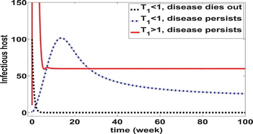On the other hand, it follows from direct calculation that the type reproduction number associated with infectious humans is (62) $T_1=k_{11}+k_{12}{k}_{21}=\frac{N}{\mu +\gamma }\left({\beta }_H\left(h_0\right)+{\beta }_L\frac{\xi \left(h_0\right)}{\delta \kappa }\right)=T_{1h}.$(62) The relationship in Equation (62(58) $R_{0w}=R_w\left(0\right)=v^{\prime }\left(h_0\right)/\zeta$(58) ) implies that this type reproduction number for the coupled system remains the same as the one for the slow system. This is due to our relatively simple formulation of the within-host dynamics, which leads to a one-to-one correspondence between the bacterial concentration in humans and that in the environment at the equilibrium state. Inclusion of human bacterial process generates a backward bifurcation not only in the coupled system but also in the epidemiological model (i.e. the slow system). The occurrence of the backward bifurcation indicates that an EE can exist and the infection can persist even if the epidemiological reproduction number is reduced to below the unity. This result underscores the challenges in the prevention and control of cholera. A numerical illustration of the backward bifurcation for the coupled system is displayed in Figure 2, which plots the number of infectious hosts as a function of time. It shows that (a) the disease can either die out (see the black dotted curve in Figure 2) or persist (see the blue dash-dot curve in Figure 2) even if the type reproduction number for infectious humans $T_1$ is less than one; (b) the full system can undergo a catastrophic transition of the disease in a sense that a small perturbation of $T_1$ from below one to above one can lead to a dramatic increase of disease prevalence. For instance, it is shown in this figure that the prevalence level in terms of the infectious human population size at the equilibrium can increase from 0 to 56 or so, as a matter of the fact that $T_1$ is slightly elevated across 1. It is worth mentioning that the initial population size of infectious persons in the case of zero-prevalence is 100, whereas that in the case of 56-prevalence is only 10.

Figure 2. Illustration of the backward bifurcation in the coupled system (1(1) $\begin{array}{rl}\frac{\mathrm{d}S}{\mathrm{d}t}& =\mu N-{\beta }_H\left(Z\right)SI-{\beta }_L\frac{SB}{\kappa +B}-\mu S+\sigma R,\\ \frac{\mathrm{d}I}{\mathrm{d}t}& ={\beta }_H\left(Z\right)SI+{\beta }_L\frac{SB}{\kappa +B}-(\gamma +\mu )I,\\ \frac{\mathrm{d}R}{\mathrm{d}t}& =\gamma I-(\mu +\sigma )R,\end{array}$(1) )–(3(3) $\frac{\mathrm{d}Z}{\mathrm{d}t}=\frac{1}{ϵ}\left(u\right(B)+v(Z)-\zeta Z),$(3) ). Each curve plots the number of infectious human hosts vs. time (in weeks). The black dotted (resp. blue dash-dot and red solid) curve shows the case where $T_1<1$ and the disease dies out (resp. the disease persists when $T_1<1$ and $T_1>1$). Note that the red curve is continuous and its peak value for the number of infectious hosts is much higher than the window displayed. Hence two disconnected pieces of red curves are shown. In this example, we set $\xi \left(Z\right)={\xi }_M$, ${\beta }_H\left(Z\right)=b_0+b_{1}Z+b_2{Z}^2$, $u\left(B\right)=B$ and $v\left(Z\right)=0$.

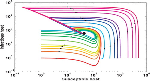
We also numerically verify the global stability of the EE for the full system when $T_1>1$ by simulating the trajectories with many different initial conditions in the biologically relevant domain. Figure 3 illustrates the projection of these trajectories onto S–I plane. It shows that the solutions converge to the EE (displayed in black dot) over time, an evidence that the EE is globally asymptotically stable.

Figure 3. Numerical verification of the global stability of the EE associated with the coupled system (1(1) $\begin{array}{rl}\frac{\mathrm{d}S}{\mathrm{d}t}& =\mu N-{\beta }_H\left(Z\right)SI-{\beta }_L\frac{SB}{\kappa +B}-\mu S+\sigma R,\\ \frac{\mathrm{d}I}{\mathrm{d}t}& ={\beta }_H\left(Z\right)SI+{\beta }_L\frac{SB}{\kappa +B}-(\gamma +\mu )I,\\ \frac{\mathrm{d}R}{\mathrm{d}t}& =\gamma I-(\mu +\sigma )R,\end{array}$(1) )–(3(3) $\frac{\mathrm{d}Z}{\mathrm{d}t}=\frac{1}{ϵ}\left(u\right(B)+v(Z)-\zeta Z),$(3) ) when $T_1>1$. This figure plots the phase portrait on S–I plane. It shows that all the trajectories with biologically meaningful initial conditions converge to the EE (displayed in the black dot).

4. Conclusion and discussion

The main contribution of this work is that we have developed a new mathematical modelling framework to study the within- and between-host dynamics of cholera, and this framework can be easily extended to other infectious diseases with free-living pathogens in the environment. The explicit linkage between disease dynamics at different scales is formulated by presuming a general representation for both the direct transmission and the pathogen shedding, and the interaction between environmental vibrios and human vibrios. Using the proposed model, we have carefully analysed the within- and between-host dynamics of the disease. Our results show that dynamics of the coupled system can be recovered by those of the slow and fast systems obtained by the fast-slow approximations. Particularly, the fast system exhibits a unique equilibrium, either infection-free or endemic, and it is globally asymptotically stable. In contrast, the slow system that captures between-host dynamic is much more complex. This subsystem can undergo a backward bifurcation, and the precise condition for the occurrence of a backward bifurcation is derived. It indicates that reducing the type reproduction number of infectious persons (or the basic reproduction number) below one is not sufficient for eradicating the disease. This finding is distinct from all previous mathematical cholera studies, in which the models only exhibit a forward bifurcation and reducing a disease threshold (e.g. the basic reproduction number) below one leads to disease extinction. The occurrence of the backward bifurcation in our model is a direct result of coupling the within- and between-host cholera dynamics.

There are several limitations in our current study. Our model does not explicitly make a distinction among human hosts, other than partially accounting for it through the ingestion rate $u\left(B\right)$ and intrinsic growth rate $v\left(Z\right)$, and thus each infected individual undergoes the same type of within-host dynamics. This assumption allows our model to be mathematically tractable, though we admit that it is unrealistic and, in reality, many factors (such as age, life style, health condition, and susceptibility level) will play together and possibly lead to very different disease dynamics for different individuals. Another limitation in our current model is the relatively simple formulation of the within-host dynamics which may not be able to capture the full complexity of the biological and pathophysiological processes inside the human body. Incorporation of the immunological modelling principles with detailed pathogen–cell interactions into our model will enrich the within-host dynamics, and lead to potentially deeper understanding of the disease mechanism. The challenge, however, is that the within-host system becomes high dimensional which will complicate the analysis for both the fast and slow system. In addition, our current model assumes that the growth of human vibrios only depends on the environmental vibrios and the intrinsic dynamics of the human vibrios. Practically, the within-host cholera dynamics may also connect to several epidemiological factors, such as the disease prevalence. We plan to investigate these issues in our future study, using both analytical and numerical approaches.

Acknowledgments

The authors would like to thank the editor and the anonymous reviewers for their suggestions that have improved this paper.

Disclosure statement

No potential conflict of interest was reported by the authors.

Additional information

Funding

This work was partially supported by a grant from the Simons Foundation (#317047 to X. Wang). J. Wang was partially supported by the National Science Foundation [grant number 1216936], [grant number 1412826] and [grant number 1520672].

Appendix 1. Type reproduction number

If disease control is targeted at a particular host type, a useful threshold is known as the type reproduction number, T. The type reproduction number defines the expected number of secondary infective cases of a particular population type caused by a typical primary case in a completely susceptible population [18,24]. It is an extension of the basic reproduction number ${\mathcal{R}}_0$.

The type reproduction number $T_i$ for the control of the target population type i is defined in Refs. [18,24] as (A1) $T_i={\mathit{e}}_i^{\mathrm{T}}\mathit{K}(\mathit{I}-(\mathit{I}-{\mathit{P}}_i)\mathit{K}{)}^{-1}{\mathit{e}}_i,$(A1) provided the spectral radius of matrix $(\mathit{I}-{\mathit{P}}_i)\mathit{K}$ is less than one. Here $\mathit{K}$ is the next generation matrix of size n. $\mathit{I}$ is the identity matrix. ${\mathit{e}}_i$ is a column vector with all zero entries except that the ith entry is 1. ${\mathit{P}}_i$ is the $n\times n$ projection matrix with all zero entries except that the $(i,i)$ entry is 1. Write $\mathit{K}=\left(k_{ij}\right)$. Particularly, if n=2, the type reproduction T can be easily defined in terms of the elements $k_{ij}$ (A2) $\begin{array}{rl}{T}_1& =k_{11}+\frac{k_{12}{k}_{21}}{1-k_{22}},\\ T_2& =k_{22}+\frac{k_{12}{k}_{21}}{1-k_{11}}.\end{array}$(A2) $T_1$ (resp. $T_2$) exists provided $k_{22}<1$ (resp. $k_{11}<1$).

Appendix 2. Model parameters and functions

The definition and base values of parameters in our cholera models are provided in Table A1. Here p (resp. y, d and h) represents a person (resp. year, day and hour).

Table A.1. Definition of model parameters.

Parameter	Definition	Value	References
N	Total population size of humans	$12,347\mathrm{p}$	[21]
μ	Natural death rate of human	$(43.5\mathrm{y}{)}^{-1}$	[34]
${\beta }_L$	Indirect transmission rate	0.011 ${\mathrm{p}}^{-1}{\mathrm{d}}^{-1}$	[21]
κ	Half saturation rate	${10}^6{\mathrm{cells}\cdot \mathrm{ml}}^{-1}$	[17]
γ	Recovery rate	$(5\mathrm{d}{)}^{-1}$	[17]
σ	Rate of host immunity loss	$(3\mathrm{y}{)}^{-1}$	[22]
δ	Bacterial death rate	$(30\mathrm{d}{)}^{-1}$	[17]
ζ	Death rate of bacteria in humans	Varied
ε	Ratio of time scale	Varied

Appendix 3. The geometric approach

We now present the main result of the geometric approach for global stability, originally developed by Li and Muldowney [19].

We consider a dynamical system (A3) $\frac{\mathrm{d}X}{\mathrm{d}t}=f\left(X\right),$(A3) where $f:D\mapsto {\mathbb{R}}^n$ is a $C^1$ function and $D\subset {\mathbb{R}}^n$ is a simply connected open set. Let $P\left(X\right)$ be a $\left(\begin{array}{c}n\\ 2\end{array}\right)\times \left(\begin{array}{c}n\\ 2\end{array}\right)$ matrix-valued $C^1$ function in D, and set $U=P_f{P}^{-1}+P{J}^{\left[2\right]}{P}^{-1},$ where $P_f$ is the derivative of P (entry-wise) along the direction of f, and $J^{\left[2\right]}$ is the second additive compound matrix of the Jacobian $J\left(X\right)=Df\left(X\right)$. Let $\mathcal{M}\left(U\right)$ be the Lozinskiǐ measure of U with respect to a matrix norm; i.e. $\mathcal{M}\left(U\right)=\underset{h\to 0^{+}}{lim}\frac{|\mathbb{I}+hU|-1}{h},$ where $\mathbb{I}$ represent the identity matrix. Define a quantity $\overline{q_2}$ as $\overline{q_2}=\underset{t\to \mathrm{\infty }}{lim sup}\underset{X_0\in K}{sup}\frac{1}{t}{\int }_0^t\mathcal{M}\left(U\right(X(s,X_0)\left)\right)\mathrm{d}s,$ where K is a compact absorbing subset of D. Then the condition $\overline{q_2}<0$ provides a Bendixson criterion in D. As a result, the following theorem holds:

Theorem A.1

Assume that there exists a compact absorbing set $K\subset D$ and the system (65(61) $R_0:=\rho \left(\mathcal{K}\right)=max\{R_{0b},R_{0w}\},$(61) ) has a unique equilibrium point $X^{\ast }$ in D. Then $X^{\ast }$ is globally asymptotically stable in D if $\overline{q_2}<0$.

References

- R.M. Anderson and R.M. May, Infectious Diseases of Humans: Dynamics and Control, Oxford University Press, Oxford, 1991.
- R. Antia, M.A. Nowak, and R.M. Anderson, Antigenic variation and the within-host dynamics of parasites, Proc. Natl. Acad. Sci. USA 93 (1996), pp. 985–989. doi: 10.1073/pnas.93.3.985
- B. Boldin and O. Diekmann, Superinfections can induce evolutionarily stable coexistence of pathogens, J. Math. Biol. 56 (2008), pp. 635–672. doi: 10.1007/s00285-007-0135-1
- V. Capasso and S.L. Paveri-Fontana, A mathematical model for the 1973 cholera epidemic in the European Mediterranean region, Rev. Epidemiol. Sante 27(2) (1979), pp. 121–132.
- V. Capasso and G. Serio, A generalization of the Kermack–Mckendrick deterministic epidemic model, Math. Biosci. 42(1) (1978), pp. 43–61. doi: 10.1016/0025-5564(78)90006-8
- A. Carpenter, Behavior in the time of cholera: Evidence from the 2008–2009 cholera outbreak in Zimbabwe, in Social Computing, Behavioral-Cultural Modeling and Prediction, J. Salerno, S.J. Yang, D. Nau, and S.-K. Chai, eds., Springer, College Park, MD, 2014, pp. 237–244.
- X. Cen, Z. Feng, and Y. Zhao, Emerging disease dynamics in a model coupling within-host and between-host systems, J. Theor. Biol. 361 (2014), pp. 141–151. doi: 10.1016/j.jtbi.2014.07.030
- R.R. Colwell, A global and historical perspective of the genus Vibrio, in The Biology of Vibrios, F.L. Thompson, B. Austin, and J. Swings, eds., ASM Press, Washington, DC, 2006, pp. 3–26.
- D. Coombs, M.A. Gilchrist, and C.L. Ball, Evaluating the importance of within- and between-host selection pressures on the evolution of chronic pathogens, Theor. Popul. Biol. 72 (2007), pp. 576–591. doi: 10.1016/j.tpb.2007.08.005
- M.C. Eisenberg, Z. Shuai, J.H. Tien, and P. van den Driessche, A cholera model in a patchy environment with water and human movement, Math. Biosci. 246(1) (2013), pp. 105–112. doi: 10.1016/j.mbs.2013.08.003
- Z. Feng, J. Velasco-Hernandez, B. Tapia-Santos, and M.C.A. Leite, A model for coupling within-host and between-host dynamics in an infectious disease, Nonlinear Dyn. 68 (2012), pp. 401–411. doi: 10.1007/s11071-011-0291-0
- Z. Feng, J. Velasco-Hernandez, and B. Tapia-Santos, A mathematical model for coupling within-host and between-host dynamics in an environmentally-driven infectious disease, Math. Biosci. 241 (2013), pp. 49–55. doi: 10.1016/j.mbs.2012.09.004
- Z. Feng, X. Cen, Y. Zhao, and J.X. Velasco-Hernandez, Coupled within-host and between-host dynamics and evolution of virulence, Math. Biosci. (2015). Available at http://dx.doi.org/10.1016/j.mbs.2015.02.01.
- W. Garira, D. Mathebula, and R. Netshikweta, A mathematical modelling framework for linked within-host and between-host dynamics for infections with free-living pathogens in the environment, Math. Biosci. 256 (2014), pp. 58–78. doi: 10.1016/j.mbs.2014.08.004
- M.A. Gilchrist and D. Coombs, Evolution of virulence: Interdependence, constraints, and selection using nested models, Theor. Popul. Biol. 69 (2006), pp. 145–153. doi: 10.1016/j.tpb.2005.07.002
- M.A. Gilchrist and A. Sasaki, Modeling host–parasite coevolution: A nested approach based on mechanistic models, J. Theor. Biol. 218 (2002), pp. 289– 308. doi: 10.1006/jtbi.2002.3076
- D.M. Hartley, J.G. Morris, and D.L. Smith, Hyperinfectivity: A critical element in the ability of V. cholerae to cause epidemics?, PLoS Med. 3 (2006), pp. 0063–0069. doi: 10.1371/journal.pmed.0030063
- J.A.P. Heesterbeek and M.G. Roberts, The type-reproduction number T in models for infectious disease control, Math. Biosci. 206 (2007), pp. 3–10. doi: 10.1016/j.mbs.2004.10.013
- M.Y. Li and J.S. Muldowney, A geometric approach to global-stability problems, SIAM J. Math. Anal. 27 (1996), pp. 1070–1083. doi: 10.1137/S0036141094266449
- N. Mideo, S. Alizon, and T. Day, Linking within- and between-host dynamics in the evolutionary epidemiology of infectious diseases, Trends Ecol. Evol. 23 (2008), pp. 511–517. doi: 10.1016/j.tree.2008.05.009
- Z. Mukandavire, S. Liao, J. Wang, H. Gaff, D.L. Smith, and J.G. Morris, Estimating the reproductive numbers for the 2008–2009 cholera outbreaks in Zimbabwe, Proc. Natl. Acad. Sci. USA 108 (2011), pp. 8767–8772. doi: 10.1073/pnas.1019712108
- R.L.M. Neilan, E. Schaefer, H. Gaff, K.R. Fister, and S. Lenhart, Modeling optimal intervention strategies for cholera, Bull. Math. Biol. 72 (2010), pp. 2004–2018. doi: 10.1007/s11538-010-9521-8
- E.J. Nelson, J.B. Harris, J.G. Morris, S.B. Calderwood, and A. Camilli, Cholera transmission: The host, pathogen and bacteriophage dynamics, Nat. Rev.: Microbiol. 7 (2009), pp. 693–702.
- M.G. Roberts and J.A.P. Heesterbeek, A new method for estimating the effort required to control an infectious disease, Proc. R. Soc. B 270 (2003), pp. 1359–1364. doi: 10.1098/rspb.2003.2339
- M. Shen, Y. Xiao, and L. Rong, Global stability of an infection-age structured HIV-1 model linking within-host and between-host dynamics, Math. Biosci. 263 (2015), pp. 37–50. doi: 10.1016/j.mbs.2015.02.003
- Z. Shuai and P. van den Driessche, Global dynamics of cholera models with differential infectivity, Math. Biosci. 234(2) (2011), pp. 118–126. doi: 10.1016/j.mbs.2011.09.003
- Z. Shuai and P. van den Driessche, Modelling and control of cholera on networks with a common water source, J. Biol. Dyn. 9(1) (2015), pp. 90–103. doi: 10.1080/17513758.2014.944226
- J.P. Tian and J. Wang, Global stability for cholera epidemic models, Math. Biosci. 232(1) (2011), pp. 31–41. doi: 10.1016/j.mbs.2011.04.001
- J.H. Tien and D.J.D. Earn, Multiple transmission pathways and disease dynamics in a waterborne pathogen model, Bull. Math. Biol. 72(6) (2010), pp. 1506–1533. doi: 10.1007/s11538-010-9507-6
- P. van den Driessche and J. Watmough, Reproduction numbers and sub-threshold endemic equilibria for compartmental models of disease transmission, Math. Biosci. 180 (2002), pp. 29–48. doi: 10.1016/S0025-5564(02)00108-6
- Y. Wang and J. Cao, Global stability of general cholera models with nonlinear incidence and removal rates, J. Franklin Inst. 352(6) (2015), pp. 2464–2485. doi: 10.1016/j.jfranklin.2015.03.030
- J. Wang and S. Liao, A generalized cholera model and epidemic–endemic analysis, J. Biol. Dyn. 6(2) (2012), pp. 568–589. doi: 10.1080/17513758.2012.658089
- J. Wang and C. Modnak, Modeling cholera dynamics with controls, Can. Appl. Math. Quart. 19(3) (2011), pp. 255–273.
- X. Wang and J. Wang, Analysis of cholera epidemics with bacterial growth and spatial movement, J. Biol. Dyn. 9 (2015), pp. 233–261. doi: 10.1080/17513758.2014.974696
- X. Wang, D. Gao, and J. Wang, Influence of human behavior on cholera dynamics, Math. Biosci. 267 (2015), pp. 41–52. doi: 10.1016/j.mbs.2015.06.009
- X. Wang, D. Posny, and J. Wang, A reaction–convection–diffusion model for cholera spatial dynamics, Discrete Continuous Dyn. Syst. Ser. B. 21(8) (2016), pp. 2785–2809.