A mathematical model for the interplay of Nosema infection and forager losses in honey bee colonies

ABSTRACT

We present a mathematical model (a) for the infection of a honey bee colony with Nosema ceranae. This is a system of five ordinary differential equations for the dependent variables healthy and infected worker bees in the hive, healthy and infected forager bees, and disease potential deposited in the hive. The model is then (b) extended to account for increased forager losses, e.g. caused by exposure to external stressors. The model is non-autonomous with periodic coefficient functions. Algebraic complexity prevents a rigorous mathematical analysis. Therefore, we resort to computer simulations in addition to some analytical results in the constant coefficient case. We investigate each of the two stressors (a) and (b) individually and jointly. Our results indicate that the combined effect of two stressors, both of which can be tolerated by the colony individually, might lead to colony failure, suggesting multi-factorial causes behind losses of honey bee colonies.

KEYWORDS:

• Forager losses
• honey bees
• mathematical model
• non-autonomous ordinary differentialequation
• Nosema ceranae

MATHEMATICS SUBJECT CLASSIFICATIONS:

• 92D25
• 92D30
• 34C60

1. Introduction

Western honey bees (Apis mellifera) have been used since antiquity for the production of honey and beeswax. While they have always played a natural role as a pollinator in food production, the agricultural sector has capitalized on this by placing honey bee hives around crop fields during blooming seasons, thereby maximizing pollination. This has allowed certain crops to be scaled upwards in production, but has also led to some agricultural sectors becoming dependent upon the use of honey bees. Indeed, a study of 107 globally traded crops found that the production of 75% of these crops were directly affected by pollinators such as honey bees. While many staple foods do not depend on pollinators for production, the absence of pollinators would restrict the variety and nutritional value of the current human diet [31].

Humanity has come to rely on the honey bee, and now has a vested interest in combating threats to the honey bee. This fact has been brought to the fore since 2006, when large numbers of colony losses were reported by beekeepers [13,24,32]. The cause or causes of this phenomenon remain unclear. However, many suggestions have been put forward, including (but not limited to) viruses, mites, pesticides, stress from hive management, and habitat loss. It has been suggested that the true cause may lie in a confluence of a number of these factors [38].

One parasite in particular, Nosema ceranae, has been implicated in colony losses on a global scale, although its exact role in these losses is debated [21]. N. ceranae is a microsporidian which has traditionally been known to infect Asian honey bees (Apis cerana) but has also been observed in A. mellifera hives. In Canadian hives, N. ceranae has been found to be more prevalent and more virulent than Nosema apis in recent years [12]. Its infective form is contained in a spore which contaminates the combs of a hive, where bees may ingest the spore while cleaning the combs [2,10]. Upon ingestion, the spore germinates, multiplies in the midgut's epithelial cells, and infects the bee, which defecates new spores onto the combs to be ingested by other bees. The infection itself has been shown to decrease the lifespans of bees once they leave the hive to forage for food [15]. Some have proposed that N. ceranae is the main cause of CCD in A. mellifera colonies [19], while others have suggested it as one of multiple stressors leading to hive failure [38].

Bee colonies have been the subject of a variety of mathematical models to study a range of phenomena in apiculture. A recent summary of these models divides them into three general categories: varroa models, used to study varroa mites, a particularly deadly pest; forager models, which include the effect of division of labour in the colony; and colony models which focus on phenomena related to the development cycle of honey bees in greater detail [4]. There is, of course, overlap between these three categories. While many disease-parasitic models have been put forward for varroa mites and the viruses they transmit (e.g. [33,39]), a burgeoning area of research lies in disease models for other honey bee diseases and parasites. These models can also contain elements of the other model categories to include the effects of bee biology and ethology. A model for the transition of bees between the two largest classes in a colony, hive worker bees and forager bees, has been proposed in [25]. The same authors later developed the model to include the effects of food stores on colony growth and to further refine the population into brood, hive bees, and forager bees [26]. This model was expanded into generic disease models in [6,27]. Both are SIR-type models, with the former modelling a disease brought into the hive by foragers and the latter modelling a disease spread by contact among healthy and infected bees and including food dynamics. While the authors propose that these models can potentially be applied to N. ceranae, neither focuses on the particular dynamics of the disease and its spread within a colony via spores that are deposited within the hive. In a similar vein, a model is proposed in [9] to study the effects of colony stress and individual bee impairment in social bee colonies, but this model focuses solely on generic stresses rather than particular diseases.

Regarding the pathology of N. ceranae, our understanding of the disease is lacking in some areas, in part because the microsporidian, and the distinction between N. apis and N. ceranae, are relatively recent discoveries. However, some studies have been conducted. In [15] estimates of the effects of N. ceranae infections on the lifespans of bees are derived. The effects of N. ceranae are compared to those of N. apis on honey bee health in [14,23]. The use of antibiotics as treatment was investigated in [42]. However, exact data on infection rates, mortality rates, and other factors have been difficult to obtain, due to the inherent structure of bee colonies and the nature of the disease.

In the following sections, we will propose a model for the spread of N. ceranae within a colony of A. mellifera. Following the traditional SIR model of disease dynamics, this model will stratify bees into healthy and infected classes, and, simultaneously, following Khoury et al. [25], into hive and forager classes. Instead of assuming direct disease transmission between infected and susceptible bees, as in previous models, we will assume that disease transmission is via an environmental reservoir of spores, i.e. Nosema spores deposited in the hive. We will then analyse this model using algebraic and computational techniques with the aim of developing a better understanding of the dynamics of the disease within the colony.

We will further extend the model to account for a second stressor that manifests itself in terms of increased forager losses, i.e. the diminished ability of foragers to return to the hive. Here, we follow the approach in [18] where this was used to include the effects of exposure of foragers to environmental pesticides when visiting treated crops. This will give insight into how these different effects work in tandem to affect a colony.

The outline of the paper is as follows: We first give in Section 2 an overview of the biology of honey bee colonies and N. ceranae to justify our model assumptions. Then we present the mathematical model. While the model in its general form is a non-autonomous model that reflects seasonal changes in honey bee biology, we present in Section 3 some analytic results for the autonomous case that help in designing and interpreting simulation results of the full model, which are presented in Section 4. Finally in Section 4.6 we investigate the potential of hive cleaning to prevent colony failure due to nosemosis and/or increased forager losses.

2. Mathematical model

2.1. Biological background

A colony of Western honey bees (A. mellifera) centres around the queen bee, which has the sole responsibility of laying eggs. The queen is tended to by female worker bees, whose population can grow in excess of 40,000 bees in Summer. Also present are hundreds of male drones which have the sole task of mating with the queen [35].

The worker bees begin their lives as eggs laid by the queen in the hive's combs. These eggs hatch into larvae which are fed by adult workers. The workers then seal the cells containing larvae with a wax cap, where they develop into pupae. When fully developed, the new worker bees emerge from the comb and cycle through various tasks including hive cleaning and protection, brood care, and tending to the queen [8,36,43]. Larger colonies correlate with higher brood production [1,29]. Newly emerged worker bees cycle through a number of tasks around the hive such as cell cleaning and brood rearing. The oldest workers leave the hive as foragers to collect nectar, pollen, and other hive materials, creating an overarching class division between hive bees and forager bees [36]. In a properly functioning colony, the rate at which bees become foragers depends on the distribution of labour within the colony and changes so that, at a given time during a foraging season, foragers compose approximately one-third of the colony [5,40]. Physiologically, it is believed that this transition is influenced by two hormones in hive bees, the juvenile hormone and vitellogenin, which are influenced by the presence of forager bees in the hive and serve to regulate the division of labour among worker bees [15].

Honey bee colonies exhibit an annual cycle of growth and decline, particularly in colder climates. A colony lies dormant in Winter as bees remain in the hive and vibrate to maintain an in-hive temperature above 10°C. In Spring, populations grow, then remain high in Summer and decrease in Autumn towards their Winter lows [35]. The average age of a bee also depends on the season and can range from as low as a 15 days in the Summer to several months in the Winter [43].

N. ceranae exists as spores on the combs of the hive until ingested by a worker bee when cleaning cells to provide cells for the queen to lay eggs. Once inside a bee, the spore germinates and reproduces. During defecation, some spores exit the bee and can be deposited on the combs to be ingested by other bees [2,10]. N. ceranae exhibits a cyclical nature where outbreaks often occur in the Spring and early Summer, apparently due to the bees' behaviour. During Winter, bees cannot leave the hive and infected bees defecate on the combs, contaminating them with spores. Because the queen bee does not lay eggs or lays only very few eggs for much of the Winter, the worker bees do not clean the combs, leading to a buildup of spores over Winter in an infected hive. As Spring approaches and the queen begins to lay eggs, the workers clean combs, causing infections [2]. As the year progresses into Summer and Fall, the spores have been found to naturally decrease in infectivity and viability [28]. During Spring, Summer, and Fall, bees are able to defecate outside the hive in good weather, though inclement weather can force bees into the hive, leading to more spores being deposited in the hive [30]. N. ceranae has been found to shorten the lifespan of bees, but the survival rates of healthy and infected bees were only seen to diverge after roughly 14 days [15], after the worker bees became foragers.

2.2. Model assumptions

Our mathematical model is based on the following assumptions:

1. We ignore events that compromise the health of the queen bee, viewing these as discrete events that are exceptions rather than rules. Thus, we assume that the queen bee does not die, or that she is replaced without affecting the colony's performance. We also assume that the queen bee is unaffected by the disease. This follows the approach in [6,25,27,33,39] and many other modelling studies.

2. Since drones do not play a substantial role in the colony's ongoing dynamics, we neglect them and focus our model solely around adult worker bees. This also follows the approach in [6,25,27,33,39], etc.

3. Given the impact the class structure has on the workings of the colony, we distinguish between hive bees and forager bees in our model, following the approach introduced in [25]. In the case of Nosema-infected hives this is particularly important, because bees get primarily infected as hive bees, e.g. during comb cleaning, whereas older bees, i.e. foragers, are more affected by it.

4. We assume that bees emerge as adult worker bees, following [25,27,33,39], rather than requiring that bees pass through larval and pupal stages. While this reduces the faithfulness of our model, it circumvents the need to include delays in our differential equations, which complicate mathematical analysis.

5. We assume that the eclosion rate for hive bees is determined by the product of the daily maximum potential eclosion rate and a measure of the colony's brood-rearing capacity, as in [11,25]. The former is determined by the average number of eggs laid per day by the queen, while the latter is a sigmoidal function, as in [11], of the total colony population. Thus, the eclosion rate can be hampered by low levels of worker bees.

6. Assuming that the primary route of transmission of Nosema is the ingestion of spores during hive cleaning, we introduce as a dependent variable the ‘environmental potential’ or ‘environmental reservoir’ of the disease, denoted E, which is a measure for the number of viable spores on the comb.

7. Hive bees emerge from their cells healthy but can become infected by ingesting spores (i.e. by uptake from the environmental reservoir) [10]. Thus, we distinguish between healthy hive bees ($H_0$) and infected hive bees ($H_1$). We assume that no new infections occur among bees once they leave the hive to forage and focus on in-hive acquisition as the primary route of transmission. Hence, we neglect the possibility that foragers acquire the disease on flowers in fields. In [20] it was suggested that this possibility exists but is very unlikely. In [17], the possibility of disease acquisition on flowers could be shown in tightly controlled laboratory experiments, but not enough quantitative information is available in the literature for parameterization in a field scale model.

8. Since infection impacts the lifespan of bees in the later stages of development [15], we assume a pronounced effect on forager life spans. Thus, we further distinguish between healthy foragers ($F_0$) and infected foragers ($F_1$), yielding four classes of bees. When leaving the hive, healthy hive bees become healthy foragers, and infected hive bees become infected foragers. We assume that the ratios at which healthy and infected bees transition are equal.

9. The infection rate of hive bees increases with the number of healthy hive bees and with the strength of the environmental potential. This relationship is linear with respect to the bees, but it saturates with respect to the environmental potential when the potential is exceedingly large. The rationale for this is that, from a biological standpoint, once a large enough number of spores exist on the combs of the hive, having additional spores will not increase the chance of any bee becoming infected. However, the number of bees infected is, of course, directly proportional to the number of bees present, i.e. partaking in hive duties.

10. Infected hive bees contribute spores to the environmental reservoir, by defecation.

11. The environmental reservoir of infective agents decreases due to natural decay (i.e. loss of viability of spores) and ingestion of spores by hive bees.

12. Since both honey bee biology and population dynamics, and Nosema disease dynamics vary between the seasons, we will assume that our parameters are time-dependent, with a periodicity of one year, as in [33].

2.3. Governing equations

Based on the above assumptions, our model reads (1) ${\dot{H}}_0=\beta \left(t\right)\frac{Z^n}{\kappa (t{)}^n+Z^n}-{\sigma }_1\left(t\right)H_0+{\sigma }_2\left(t\right)\frac{F}{Z}{F}_0-{\eta }_0\left(t\right)H_0-\alpha \left(t\right)H_0\frac{E}{\lambda \left(t\right)+E},$(1) (2) ${\dot{H}}_1=-{\sigma }_1\left(t\right)H_1+{\sigma }_2\left(t\right)\frac{F}{Z}{F}_1-{\eta }_1\left(t\right)H_1+\alpha \left(t\right)H_0\frac{E}{\lambda \left(t\right)+E},$(2) (3) ${\dot{F}}_0={\sigma }_1\left(t\right)H_0-{\sigma }_2\left(t\right)\frac{F}{Z}{F}_0-{\phi }_0\left(t\right)F_0,$(3) (4) ${\dot{F}}_1={\sigma }_1\left(t\right)H_1-{\sigma }_2\left(t\right)\frac{F}{Z}{F}_1-{\phi }_1\left(t\right)F_1,$(4) (5) $\dot{E}=\gamma \left(t\right)H_1-\delta \left(t\right)E-\tilde{\alpha }\left(t\right)H_0\frac{E}{\lambda \left(t\right)+E},$(5) where we use the shorthand notations (6) $H:=H_0+H_1,F:=F_0+F_1,Z:=H+F.$(6) All parameters are time-dependent, non-negative, and assumed to be periodic with periods of one year to reflect seasonal changes. Our model is based on the hive-forager model presented in [25], although we make some alterations and expansions.

In Equation (1(1) ${\dot{H}}_0=\beta \left(t\right)\frac{Z^n}{\kappa (t{)}^n+Z^n}-{\sigma }_1\left(t\right)H_0+{\sigma }_2\left(t\right)\frac{F}{Z}{F}_0-{\eta }_0\left(t\right)H_0-\alpha \left(t\right)H_0\frac{E}{\lambda \left(t\right)+E},$(1) ), the parameter β is the maximum emergence rate of healthy adult hive bees. κ is the brood maintenance coefficient as introduced in [11]; for the Hill exponent n we will generally take $n\ge 2$. Then, if $Z\ll \kappa$ very few new bees emerge, while for $Z\gg \kappa$ emergence is close to maximal rate. This sigmoidal form of the emergence rate, adapted from [11], is a modification from the original hive-forager model [25], which had simple Holling Type 2 saturation, i.e. assuming that at low bee populations emergence is proportional to the number of worker bees. Bees are eusocial insects and colonies cannot exist in the long term with exceedingly low populations, therefore we consider our Holling Type 3 variant ecologically more realistic.

We include the terms containing ${\eta }_0$, ${\eta }_1$, ${\phi }_0$, and ${\phi }_1$ in Equations (1(1) ${\dot{H}}_0=\beta \left(t\right)\frac{Z^n}{\kappa (t{)}^n+Z^n}-{\sigma }_1\left(t\right)H_0+{\sigma }_2\left(t\right)\frac{F}{Z}{F}_0-{\eta }_0\left(t\right)H_0-\alpha \left(t\right)H_0\frac{E}{\lambda \left(t\right)+E},$(1) )–(4(4) ${\dot{F}}_1={\sigma }_1\left(t\right)H_1-{\sigma }_2\left(t\right)\frac{F}{Z}{F}_1-{\phi }_1\left(t\right)F_1,$(4) ) to model the deaths of their respective classes. Including death terms for hive bees is a modification of Khoury et al. [25]. While the natural death terms for hive bees may be negligible compared to the rate at which hive bees become foragers, they must be dominating in Winter when all bees revert to being hive bees and no hive bees become foragers.

In Equations (1(1) ${\dot{H}}_0=\beta \left(t\right)\frac{Z^n}{\kappa (t{)}^n+Z^n}-{\sigma }_1\left(t\right)H_0+{\sigma }_2\left(t\right)\frac{F}{Z}{F}_0-{\eta }_0\left(t\right)H_0-\alpha \left(t\right)H_0\frac{E}{\lambda \left(t\right)+E},$(1) )–(4(4) ${\dot{F}}_1={\sigma }_1\left(t\right)H_1-{\sigma }_2\left(t\right)\frac{F}{Z}{F}_1-{\phi }_1\left(t\right)F_1,$(4) ), the terms with ${\sigma }_1$ and ${\sigma }_2$ describe the transition (and possibly back reversion) of hive bees to forager bees, sometimes referred to as recruitment terms in the honeybee modelling literature. Hive bees become foragers at the nominal rate ${\sigma }_1$; the ${\sigma }_2$ term accounts for a reduction of forager recruitment and possible reversion if the hive–forager bee balance is perturbed. In [25] this was modelled by a social inhibition term. Applying the same idea to the system at hand, however, does not guarantee positivity of the solutions, due to the division of forager bees into two sub-classes, $F_0$ and $F_1$. Therefore, we model this effect by transfer from the forager compartments into the corresponding hive compartments, at rates that depend on the fraction of foragers among the worker bees. A discussion and comparison of the hive–forager transition terms used here with those of Khoury et al. [25] for the case of a colony without diseases is given in the appendix.

In Equations (1(1) ${\dot{H}}_0=\beta \left(t\right)\frac{Z^n}{\kappa (t{)}^n+Z^n}-{\sigma }_1\left(t\right)H_0+{\sigma }_2\left(t\right)\frac{F}{Z}{F}_0-{\eta }_0\left(t\right)H_0-\alpha \left(t\right)H_0\frac{E}{\lambda \left(t\right)+E},$(1) ), (2) the term $\alpha \left(E/(\lambda +E)\right)H_0$ describes the acquisition of the disease by healthy hive bees, which then become infected. The acquisition rate depends on the current level of the environmental reservoir, i.e. the Nosema spores in the hive. α is the maximum infection rate, while λ is the half-saturation constant for the environmental potential.

In (5(5) $\dot{E}=\gamma \left(t\right)H_1-\delta \left(t\right)E-\tilde{\alpha }\left(t\right)H_0\frac{E}{\lambda \left(t\right)+E},$(5) ), parameter γ is the rate of spore deposition by infected hive bees; δ is the rate at which the spores loose viability; $\tilde{\alpha }$ is the maximum rate at which spores are taken up from the reservoir by worker bees due to ingestion. We assume here that spore uptake is proportional to newly acquired infections.

Proposition 2.1: (Existence, uniqueness, non-negativity and boundeness):

Let $\eta \left(t\right):=min\left\{{\eta }_0\right(t),{\eta }_1(t),{\phi }_0(t),{\phi }_1(t\left)\right\}$. The initial value problem of (1(1) ${\dot{H}}_0=\beta \left(t\right)\frac{Z^n}{\kappa (t{)}^n+Z^n}-{\sigma }_1\left(t\right)H_0+{\sigma }_2\left(t\right)\frac{F}{Z}{F}_0-{\eta }_0\left(t\right)H_0-\alpha \left(t\right)H_0\frac{E}{\lambda \left(t\right)+E},$(1) )–(6(6) $H:=H_0+H_1,F:=F_0+F_1,Z:=H+F.$(6) ) with non-negative initial data in the set $\mathcal{K}:=\left\{\right(H_0,H_1,F_0,F_1,E)\in {\mathbb{R}}^5:H_0\ge 0,H_1\ge 0,F_0\ge 0,F_1\ge 0,H_0+H_1+F_0+F_1>0,E\ge 0\}$ possesses a unique solution which remains in $\mathcal{K}$ for all t>0 and is bounded by (7) $0\le Z\left(t\right)\le \exp \left(-{\int }_0^t\eta \left(\tau \right)\mathrm{d}\tau \right)\left({\int }_0^t\exp \left({\int }_0^{\tau }\eta \left(s\right)\mathrm{d}s\right)\beta \left(\tau \right)\mathrm{d}\tau +Z\left(0\right)\right),$(7) where $Z\left(t\right):=H_0\left(t\right)+H_1\left(t\right)+F_0\left(t\right)+F_1\left(t\right)$ and (8) $0\le E\left(t\right)\le \exp \left(-{\int }_0^t\delta \left(\tau \right)\mathrm{d}\tau \right)\left({\int }_0^t\exp \left({\int }_0^{\tau }\delta \left(s\right)\mathrm{d}s\right)\gamma \left(\tau \right)Z\left(\tau \right)\mathrm{d}\tau +E\left(0\right)\right).$(8)

Proof.

Note that $|F/Z|<1$. Non-negativity of solutions follows with the tangent condition. Existence and uniqueness follow from the Lipschitz condition. From Equations (1(1) ${\dot{H}}_0=\beta \left(t\right)\frac{Z^n}{\kappa (t{)}^n+Z^n}-{\sigma }_1\left(t\right)H_0+{\sigma }_2\left(t\right)\frac{F}{Z}{F}_0-{\eta }_0\left(t\right)H_0-\alpha \left(t\right)H_0\frac{E}{\lambda \left(t\right)+E},$(1) )–(4(4) ${\dot{F}}_1={\sigma }_1\left(t\right)H_1-{\sigma }_2\left(t\right)\frac{F}{Z}{F}_1-{\phi }_1\left(t\right)F_1,$(4) ), we have then $\begin{array}{rl}\dot{Z}& =\beta \left(t\right)\frac{Z^n}{\kappa (t{)}^n+Z^n}-\left[{\eta }_0\right(t)H_0+{\eta }_1(t)H_1+{\phi }_0(t)F_0+{\phi }_1(t\left)F_1\right]\\ & \le \beta \left(t\right)-\eta \left(t\right)Z.\end{array}$ Assertion (7(7) $0\le Z\left(t\right)\le \exp \left(-{\int }_0^t\eta \left(\tau \right)\mathrm{d}\tau \right)\left({\int }_0^t\exp \left({\int }_0^{\tau }\eta \left(s\right)\mathrm{d}s\right)\beta \left(\tau \right)\mathrm{d}\tau +Z\left(0\right)\right),$(7) ) follows then by the comparison theorem for ordinary initial value problems [41]. Similarly, from Equation (5(5) $\dot{E}=\gamma \left(t\right)H_1-\delta \left(t\right)E-\tilde{\alpha }\left(t\right)H_0\frac{E}{\lambda \left(t\right)+E},$(5) ), we have the differential inequality $\dot{E}\le \gamma \left(t\right)Z\left(t\right)-\delta \left(t\right)E$ from which we obtain Equation (8(8) $0\le E\left(t\right)\le \exp \left(-{\int }_0^t\delta \left(\tau \right)\mathrm{d}\tau \right)\left({\int }_0^t\exp \left({\int }_0^{\tau }\delta \left(s\right)\mathrm{d}s\right)\gamma \left(\tau \right)Z\left(\tau \right)\mathrm{d}\tau +E\left(0\right)\right).$(8) ).

3. Results: autonomous case

We begin the investigation of our model with an analysis of the autonomous case. While this is quantitatively an unrealistic simplification of the problem, it allows qualitative insight into the interplay of various ingredients of the model. The results here will also aid in the design and interpretation of simulation results of the full, time-dependent model.

Proposition 3.1 (Trivial Equilibrium)

Consider the system with constant positive parameters, (9) ${\dot{H}}_0=\beta \frac{Z^n}{{\kappa }^n+Z^n}-{\sigma }_1{H}_0+{\sigma }_2\frac{F}{Z}{F}_0-{\eta }_0{H}_0-\alpha H_0\frac{E}{\lambda +E},$(9) (10) ${\dot{H}}_1=-{\sigma }_1{H}_1+{\sigma }_2\frac{F}{Z}{F}_1-{\eta }_1{H}_1+\alpha H_0\frac{E}{\lambda +E},$(10) (11) ${\dot{F}}_0={\sigma }_1{H}_0-{\sigma }_2\frac{F}{Z}{F}_0-{\phi }_0{F}_0,$(11) (12) ${\dot{F}}_1={\sigma }_1{H}_1-{\sigma }_2\frac{F}{Z}{F}_1-{\phi }_1{F}_1,$(12) (13) $\dot{E}=\gamma H_1-\delta E-\tilde{\alpha }{H}_0\frac{E}{\lambda +E},$(13) where $F:=F_0+F_1,$ $Z:=H_0+H_1+F_0+F_1$. For given $\zeta >0,$ define the set ${\mathcal{K}}_{\zeta }:=\left\{\right(H_0,H_1,F_0,F_1,E)\in {\mathbb{R}}^5:H_0\ge 0,H_1\ge 0,F_0\ge 0,F_1\ge 0,0\le H_0+H_1+F_0+F_1\le \zeta ,E\ge 0\}$. There is a ${\zeta }_0>0$ such that ${\mathcal{K}}_{\zeta }$ is positively invariant for all $\zeta <{\zeta }_0$ and $\underset{t\to \mathrm{\infty }}{lim}\left(H_0\right(t),H_1(t),F_0(t),F_1(t),E(t){)}^{\mathrm{T}}=(0,0,0,0,0{)}^{\mathrm{T}}$ for all solutions with initial data in ${\mathcal{K}}_{{\zeta }_0}$.

Proof.

Adding Equations (9(9) ${\dot{H}}_0=\beta \frac{Z^n}{{\kappa }^n+Z^n}-{\sigma }_1{H}_0+{\sigma }_2\frac{F}{Z}{F}_0-{\eta }_0{H}_0-\alpha H_0\frac{E}{\lambda +E},$(9) )–(12(12) ${\dot{F}}_1={\sigma }_1{H}_1-{\sigma }_2\frac{F}{Z}{F}_1-{\phi }_1{F}_1,$(12) ), we have with $\eta :=min\{{\eta }_0,{\eta }_1,{\phi }_0,{\phi }_1\}>0$ the differential inequality $\dot{Z}=\beta \frac{Z^n}{{\kappa }^n+Z^n}-{\eta }_0{H}_0-{\eta }_1{H}_1-{\phi }_0{F}_0-{\phi }_1{F}_1\le \beta \frac{Z^n}{{\kappa }^n+Z^n}-\eta Z.$ Consider now the differential equation (14) $\dot{Y}=\beta \frac{Y^n}{{\kappa }^n+Y^n}-\eta Y.$(14) By comparison theorems, cf. [41], the solutions of Equation (14(14) $\dot{Y}=\beta \frac{Y^n}{{\kappa }^n+Y^n}-\eta Y.$(14) ) with initial data $Y\left(0\right)=Z\left(0\right)$ give upper bounds on $Z\left(t\right)$, i.e. $0\le Z\left(t\right)\le Y\left(t\right)$. This differential equation has the trivial equilibrium $Y_0^{\ast }=0$. It is easy to verify, by linearization, that $Y_0^{\ast }$ is asymptotically stable for n>1. Thus, for small enough Y, we have $Y\to 0$ as $t\to 0$. Hence, for small enough ${\zeta }^{\ast }$ all solution that start in ${\mathcal{K}}_{{\zeta }^{\ast }}$ converge to the trivial equilibrium.

Lastly, as $Z\to 0$, we find $\dot{E}\to -\delta E$, implying that $E\to 0$.

Thus, the trivial, ‘empty-hive’, equilibrium is asymptotically stable for $0\le Z<{\zeta }^{\ast }$, $E\in \mathbb{R}$.

Remark 3.2

The stability of the empty hive is caused by an Allee effect.

Proof.

To see this, consider the dynamics of Equation (14(14) $\dot{Y}=\beta \frac{Y^n}{{\kappa }^n+Y^n}-\eta Y.$(14) ). Besides the trivial equilibrium, by Descartes' rule of signs, it can have two more positive equilibria, which are found as roots of the polynomial $\mathrm{\Phi }\left(Y\right)=\beta Y^{n-1}-\delta ({\kappa }^n+Y^n).$ Obviously, $\mathrm{\Phi }\left(0\right)<0$. On the other hand, $\mathrm{\Phi }\left(Y\right)<0$ for sufficiently large Y. Thus, for positive roots to exist, the maximum of Φ on the positive half line must be positive. This maximum is found at $\tilde{Y}=\left(\beta /\delta \right)\left((n-1)/n\right)$. By substitution we obtain $\mathrm{\Phi }\left(\tilde{Y}\right)=\beta {\left(\frac{\beta }{\delta }\frac{n-1}{n}\right)}^{n-1}\left(1-\frac{n-1}{n}\right)-\delta {\kappa }^n>0,$ if (15) $\kappa <\frac{\beta }{\delta n}(n-1{)}^{(n-1)/n}.$(15) Under this condition, Equation (14(14) $\dot{Y}=\beta \frac{Y^n}{{\kappa }^n+Y^n}-\eta Y.$(14) ) has two more positive equilibria $Y_{1,2}^{\ast }$ with $Y_0^{\ast }<Y_1^{\ast }<\tilde{Y}<Y_2^{\ast }$. It is easy to verify that $Y_1^{\ast }$ is unstable while $Y_2^{\ast }$ is asymptotically stable. Hence, for initial data $Y\left(0\right)<Y_1^{\ast }$, the solutions of Equation (14(14) $\dot{Y}=\beta \frac{Y^n}{{\kappa }^n+Y^n}-\eta Y.$(14) ) converge to extinction, whereas for $Y\left(0\right)>Y_1^{\ast }$ they converge to $Y_2^{\ast }$, which establishes an Allee effect. Any ${\zeta }_0<Y_1^{\ast }$ can be chosen in Proposition 3.1.

Proposition 3.3 (Disease-free equilibria, existence):

Consider again system (9(9) ${\dot{H}}_0=\beta \frac{Z^n}{{\kappa }^n+Z^n}-{\sigma }_1{H}_0+{\sigma }_2\frac{F}{Z}{F}_0-{\eta }_0{H}_0-\alpha H_0\frac{E}{\lambda +E},$(9) )–(13(13) $\dot{E}=\gamma H_1-\delta E-\tilde{\alpha }{H}_0\frac{E}{\lambda +E},$(13) ) with positive constant parameters. Disease-free equilibria of the form $(H_0^{\ast },0,F_0^{\ast },0,0)$ with $H_0^{\ast }>0$ and $F_0^{\ast }>0$ satisfy $F_0^{\ast }=G{H}_0^{\ast }$ with $G:=\frac{({\sigma }_1-{\phi }_0)+\sqrt{({\sigma }_1+{\phi }_0{)}^2+4{\sigma }_1{\sigma }_2}}{2({\sigma }_1+{\phi }_0)}.$ Two such equilibria $(H_{0,1}^{\ast },0,G{H}_{0,1}^{\ast },0,0)$ and $(H_{0,2}^{\ast },0,G{H}_{0,2}^{\ast },0,0)$ exist if $\kappa <(n-1{)}^{-1/n}\left[\frac{\beta (G+1)}{({\eta }_0+{\phi }_{0}G)}\frac{n-1}{n}\right],$ none if the inequality is reversed. If the equilibria exist, then $0<H_{0,1}^{\ast }<\frac{n-1}{n}\frac{\beta }{{\eta }_0+{\phi }_{0}G}<H_{0,2}^{\ast }.$

Proof.

For a disease-free equilibrium with $H_1^{\ast }=F_1^{\ast }=E^{\ast }=0$, we have immediately $\dot{H_1}=\dot{F_1}=\dot{E}=0$. For $H_0$ and $F_0$ we have (16) ${\dot{H}}_0=\beta \frac{(H_0^{\ast }+F_0^{\ast }{)}^n}{{\kappa }^n+(H_0^{\ast }+F_0^{\ast }{)}^n}-{\eta }_0{H}_0^{\ast }-{\sigma }_1{H}_0^{\ast }+{\sigma }_2\frac{F_0^{\ast 2}}{(H_0^{\ast }+F_0^{\ast })}=0,$(16) (17) ${\dot{F}}_0={\sigma }_1{H}_0^{\ast }-{\sigma }_2\frac{F_0^{\ast 2}}{(H_0^{\ast }+F_0^{\ast })}-{\phi }_0{F}_0^{\ast }=0.$(17) From (17) we obtain $0={\sigma }_1{H}_0^{\ast 2}+{\sigma }_1{H}_0^{\ast }{F}_0^{\ast }-{\sigma }_2{F}_0^{\ast 2}-{\phi }_0{F}_0^{\ast 2}-{\phi }_0{H}_0^{\ast }{F}_0^{\ast }.$ Solving for $F_0^{\ast }$ we have $F_0^{\ast }=\frac{({\sigma }_1-{\phi }_0)\pm \sqrt{({\sigma }_1-{\phi }_0{)}^2+4{\sigma }_1({\sigma }_2+{\phi }_0)}}{2({\sigma }_1+{\phi }_0)}{H}_0^{\ast }.$ Since positivity is required, we can ignore the lower branch and obtain, after re-arranging, with (18) $G:=\frac{({\sigma }_1-{\phi }_0)+\sqrt{({\sigma }_1+{\phi }_0{)}^2+4{\sigma }_1{\sigma }_2}}{2({\sigma }_1+{\phi }_0)}$(18) that all positive disease-free equilibria satisfy (19) $F_0^{\ast }=G{H}_0^{\ast }.$(19) Adding Equations (16(16) ${\dot{H}}_0=\beta \frac{(H_0^{\ast }+F_0^{\ast }{)}^n}{{\kappa }^n+(H_0^{\ast }+F_0^{\ast }{)}^n}-{\eta }_0{H}_0^{\ast }-{\sigma }_1{H}_0^{\ast }+{\sigma }_2\frac{F_0^{\ast 2}}{(H_0^{\ast }+F_0^{\ast })}=0,$(16) ) and (17(17) ${\dot{F}}_0={\sigma }_1{H}_0^{\ast }-{\sigma }_2\frac{F_0^{\ast 2}}{(H_0^{\ast }+F_0^{\ast })}-{\phi }_0{F}_0^{\ast }=0.$(17) ), we obtain (20) $0=\beta \frac{(H_0^{\ast }+F_0^{\ast }{)}^n}{{\kappa }^n+(H_0^{\ast }+F_0^{\ast }{)}^n}-{\eta }_0{H}_0^{\ast }-{\phi }_0{F}_0^{\ast }.$(20) Substituting Equation (19(19) $F_0^{\ast }=G{H}_0^{\ast }.$(19) ) into this relationship and rearranging, we find that $H_0^{\ast }>0$ is a positive root of the polynomial of degree n (21) $\mathrm{\Phi }\left(H\right)=\beta (G+1{)}^n{H}^{n-1}-({\eta }_0+{\phi }_{0}G){\kappa }^n-({\eta }_0+{\phi }_{0}G\left)\right(G+1{)}^n{H}^n.$(21) By Descartes' rule of signs, there are none or two such positive roots, depending on parameters. The calculations are the same as in Remark 3.2. We have $\mathrm{\Phi }\left(0\right)<0$ and $\mathrm{\Phi }\left(H\right)<0$ for sufficiently large H. Positive roots exist if the maximum of Φ is positive. The maximum is attained for (22) $\tilde{H}=\frac{n-1}{n}\frac{\beta }{{\eta }_0+{\phi }_{0}G}.$(22) We have then (23) $\mathrm{\Phi }\left(\tilde{H}\right)=\left(\frac{1}{n-1}{\left[\frac{\beta (G+1)}{({\eta }_0+{\phi }_{0}G)}\frac{n-1}{n}\right]}^n-{\kappa }^n\right)({\eta }_0+{\phi }_{0}G)>0.$(23) Hence two positive disease-free equilibria $(H_{0,1}^{\ast },G{H}_{0,1}^{\ast })$ and $(H_{0,2}^{\ast },G{H}_{0,2}^{\ast })$ with $0<H_{0,1}^{\ast }<\tilde{H}<H_{0,2}^{\ast }$ exist if (24) $\kappa <(n-1{)}^{-1/n}\left[\frac{\beta (G+1)}{({\eta }_0+{\phi }_{0}G)}\frac{n-1}{n}\right].$(24)

The analysis of the stability of disease-free equilibria by linearization becomes rather cumbersome, owing to the high number of parameters, the non-linearity of the eclosion terms, and the high dimensionality of the state space.

Lemma 3.4 (Disease-free equilibrium stability condition):

Assume $(H_0^{\ast },0,G{H}_0^{\ast },0,0)$ is a disease-free equilibrium as per Proposition 3.3. If the inequalities $\gamma <{\eta }_1,(\alpha -\tilde{\alpha })H_0^{\ast }<\delta \lambda ,\frac{n\beta {\kappa }^n(G+1{)}^{n-1}{H}_0^{\ast (n-1)}}{({\kappa }^n+(G+1{)}^n{H}_0^{\ast n}{)}^2}<min\{{\eta }_0,{\phi }_0\},$ are satisfied, then such a disease-free equilibrium is asymptotically stable.

Proof.

To investigate the stability of such equilibria, we first rearrange the system by swapping the second and third equations, and for shorthand, set Z=H+F: $\begin{array}{rl}{\dot{H}}_0& =\beta \frac{Z^n}{{\kappa }^n+Z^n}-{\sigma }_1{H}_0+{\sigma }_2\frac{F}{Z}{F}_0-{\eta }_0{H}_0-\alpha H_0\frac{E}{\lambda +E},\\ {\dot{F}}_0& =+{\sigma }_1{H}_0-{\sigma }_2\frac{F}{Z}{F}_0-{\phi }_0{F}_0,\\ {\dot{H}}_1& =-{\sigma }_1{H}_1+{\sigma }_2\frac{F}{Z}{F}_1-{\eta }_1{H}_1+\alpha H_0\frac{E}{\lambda +E},\\ {\dot{F}}_1& =+{\sigma }_1{H}_1-{\sigma }_2\frac{F}{Z}{F}_1-{\phi }_1{F}_1,\\ \dot{E}& =\gamma H_1-\delta E-\tilde{\alpha }{H}_0\frac{E}{\lambda +E}.\end{array}$ This does not affect the values of the disease-free equilibrium, now written $(H_0^{\ast },F_0^{\ast },H_1^{\ast },F_1^{\ast },E^{\ast })=(H_0^{\ast },F_0^{\ast },0,0,0)$. Linearizing the system around the disease-free equilibrium, we obtain the Jacobian $\begin{array}{r}J=\left|\begin{array}{ccc}\frac{n\beta {\kappa }^n{Z}_0^{\ast (n-1)}}{({\kappa }^n+Z_0^{\ast n}{)}^2}-{\sigma }_1-{\sigma }_2\frac{F_0^{\ast 2}}{Z_0^{\ast 2}}-{\eta }_0& \frac{n\beta {\kappa }^n{Z}_0^{\ast (n-1)}}{({\kappa }^n+Z_0^{\ast n}{)}^2}+{\sigma }_2\frac{F_0^{\ast 2}+2H_0^{\ast }{F}_0^{\ast }}{Z_0^{\ast 2}}& \frac{n\beta {\kappa }^n{Z}_0^{\ast (n-1)}}{({\kappa }^n+Z_0^{\ast n}{)}^2}-{\sigma }_2\frac{F_0^{\ast 2}}{Z_0^{\ast 2}}\\ {\sigma }_1+{\sigma }_2\frac{F_0^{\ast 2}}{Z_0^{\ast 2}}& -{\sigma }_2\frac{F_0^{\ast 2}+2H_0^{\ast }{F}_0^{\ast }}{Z_0^{\ast 2}}-{\phi }_0& {\sigma }_2\frac{F_0^{\ast 2}}{Z_0^{\ast 2}}\\ 0& 0& -{\sigma }_1-{\eta }_1\\ 0& 0& {\sigma }_1\\ 0& 0& \gamma \end{array}\right.\left.\begin{array}{cc}\frac{n\beta {\kappa }^n{Z}_0^{\ast (n-1)}}{({\kappa }^n+Z_0^{\ast n}{)}^2}+{\sigma }_2\frac{H_0^{\ast }{F}_0^{\ast }}{Z_0^{\ast 2}}& -\frac{\alpha }{\lambda }{H}_0^{\ast }\\ -{\sigma }_2\frac{H_0^{\ast }{F}_0^{\ast }}{Z_0^{\ast 2}}& 0\\ {\sigma }_2\frac{F_0^{\ast }}{Z_0^{\ast }}& \frac{\alpha }{\lambda }{H}_0^{\ast }\\ -{\sigma }_2\frac{F_0^{\ast }}{Z_0^{\ast }}-{\phi }_1& 0\\ 0& -\delta -\frac{\tilde{\alpha }}{\lambda }{H_0}^{\ast }\end{array}\right|\end{array}$ where $Z_0^{\ast }=H_0^{\ast }+F_0^{\ast }$.

With Equation (19(19) $F_0^{\ast }=G{H}_0^{\ast }.$(19) ), we have that $Z_0^{\ast }=(G+1)H_0^{\ast }=\left((G+1)/G\right)F_0^{\ast }$, hence $\frac{F_0^{\ast }}{Z_0^{\ast }}=\frac{G}{G+1},\frac{H_0^{\ast }{F}_0^{\ast }}{Z_0^{\ast 2}}=\frac{G}{(G+1{)}^2},\frac{F_0^{\ast 2}+2H_0^{\ast }{F}_0^{\ast }}{Z_0^{\ast 2}}=\frac{G^2+2G}{(G+1{)}^2}.$ Furthermore, we have (25) $\frac{n\beta {\kappa }^n{Z}_0^{\ast (n-1)}}{({\kappa }^n+Z_0^{\ast n}{)}^2}=\frac{n\beta {\kappa }^n(G+1{)}^{(n-1)}{H}_0^{\ast (n-1)}}{({\kappa }^n+(G+1{)}^n{H}_0^{\ast n}{)}^2}.$(25) We define the function (26) $B\left(H\right):=\frac{n\beta {\kappa }^n(G+1{)}^{(n-1)}{H}^{n-1}}{({\kappa }^n+(G+1{)}^n{H}^n{)}^2}.$(26) This allows us to re-write the Jacobian as (27) $\begin{array}{rlr}J& =\left|\begin{array}{ccc}B\left(H_0^{\ast }\right)-{\sigma }_1-{\sigma }_2{\left(\frac{G}{G+1}\right)}^2-{\eta }_0& B\left(H_0^{\ast }\right)+{\sigma }_2\frac{G^2+2G}{(G+1{)}^2}& B\left(H_0^{\ast }\right)-{\sigma }_2{\left(\frac{G}{G+1}\right)}^2\\ {\sigma }_1+{\sigma }_2{\left(\frac{G}{G+1}\right)}^2& -{\sigma }_2\frac{G^2+2G}{(G+1{)}^2}-{\phi }_0& {\sigma }_2{\left(\frac{G}{G+1}\right)}^2\\ 0& 0& -{\sigma }_1-{\eta }_1\\ 0& 0& {\sigma }_1\\ 0& 0& \gamma \end{array}\right.& \left.\begin{array}{cc}B\left(H_0^{\ast }\right)+{\sigma }_2\frac{G}{(G+1{)}^2}& -\frac{\alpha }{\lambda }{H}_0^{\ast }\\ -{\sigma }_2\frac{G}{(G+1{)}^2}& 0\\ {\sigma }_2\frac{G}{G+1}& \frac{\alpha }{\lambda }{H}_0^{\ast }\\ -{\sigma }_2\frac{G}{G+1}-{\phi }_1& 0\\ 0& -\delta -\frac{\tilde{\alpha }}{\lambda }{H}_0^{\ast }\end{array}\right|.\end{array}$(27)

This is a block upper triangular matrix of the form $J=\left|\begin{array}{cc}A& B\\ 0& C\end{array}\right|$. Since the spectrum of J is the union of the spectra of the diagonal blocks A and C [22], we need only guarantee that the eigenvalues of A and C have negative real parts to ensure stability of the system around the disease-free equilibrium. Applying Gershgorin's theorem, cf [22], to these two submatrices, we find that the eigenvalues of C are in the negative half-plane when $\gamma <{\eta }_1$, $0<{\phi }_1$ (which is always true, given our assumption of positive parameters), and $(\alpha -\tilde{\alpha })H_0^{\ast }<\delta \lambda$. The eigenvalues of A are in the negative half-plane when $B\left(H_0^{\ast }\right)<{\eta }_0$ and $B\left(H_0^{\ast }\right)<{\phi }_0$.

The following result shows under which conditions on parameters an asymptotically stable equilibrium of the underlying population model inherits stability in the model with disease.

Remark 3.5

It is easy to verify that every solution $(H,F)$ of the underlying population model without disease (28) $\dot{H}=\beta \frac{Z^n}{{\kappa }^n+Z^n}-{\sigma }_{1}H+{\sigma }_2\frac{F^2}{Z}-{\eta }_{0}H,$(28) (29) $\dot{F}={\sigma }_{1}H-{\sigma }_2\frac{F^2}{Z}-{\phi }_{0}F$(29) with Z=F+H defines a solution $(H,0,F,0,0)$ of Equations (9(9) ${\dot{H}}_0=\beta \frac{Z^n}{{\kappa }^n+Z^n}-{\sigma }_1{H}_0+{\sigma }_2\frac{F}{Z}{F}_0-{\eta }_0{H}_0-\alpha H_0\frac{E}{\lambda +E},$(9) )–(13(13) $\dot{E}=\gamma H_1-\delta E-\tilde{\alpha }{H}_0\frac{E}{\lambda +E},$(13) ). If $(H^{\ast },F^{\ast })$ is an asymptotically stable equilibrium of this model, then the condition of Lemma 3.4 for its stability under (9(9) ${\dot{H}}_0=\beta \frac{Z^n}{{\kappa }^n+Z^n}-{\sigma }_1{H}_0+{\sigma }_2\frac{F}{Z}{F}_0-{\eta }_0{H}_0-\alpha H_0\frac{E}{\lambda +E},$(9) )–(13(13) $\dot{E}=\gamma H_1-\delta E-\tilde{\alpha }{H}_0\frac{E}{\lambda +E},$(13) ) reduces to $\gamma <{\eta }_1,(\alpha -\tilde{\alpha })H^{\ast }<\delta \lambda .$

Proof.

The Jacobian of Equations (28(28) $\dot{H}=\beta \frac{Z^n}{{\kappa }^n+Z^n}-{\sigma }_{1}H+{\sigma }_2\frac{F^2}{Z}-{\eta }_{0}H,$(28) )–(29(29) $\dot{F}={\sigma }_{1}H-{\sigma }_2\frac{F^2}{Z}-{\phi }_{0}F$(29) ) in a non-trivial equilibrium is the matrix block A of the matrix J in Equation (27(27) $\begin{array}{rlr}J& =\left|\begin{array}{ccc}B\left(H_0^{\ast }\right)-{\sigma }_1-{\sigma }_2{\left(\frac{G}{G+1}\right)}^2-{\eta }_0& B\left(H_0^{\ast }\right)+{\sigma }_2\frac{G^2+2G}{(G+1{)}^2}& B\left(H_0^{\ast }\right)-{\sigma }_2{\left(\frac{G}{G+1}\right)}^2\\ {\sigma }_1+{\sigma }_2{\left(\frac{G}{G+1}\right)}^2& -{\sigma }_2\frac{G^2+2G}{(G+1{)}^2}-{\phi }_0& {\sigma }_2{\left(\frac{G}{G+1}\right)}^2\\ 0& 0& -{\sigma }_1-{\eta }_1\\ 0& 0& {\sigma }_1\\ 0& 0& \gamma \end{array}\right.& \left.\begin{array}{cc}B\left(H_0^{\ast }\right)+{\sigma }_2\frac{G}{(G+1{)}^2}& -\frac{\alpha }{\lambda }{H}_0^{\ast }\\ -{\sigma }_2\frac{G}{(G+1{)}^2}& 0\\ {\sigma }_2\frac{G}{G+1}& \frac{\alpha }{\lambda }{H}_0^{\ast }\\ -{\sigma }_2\frac{G}{G+1}-{\phi }_1& 0\\ 0& -\delta -\frac{\tilde{\alpha }}{\lambda }{H}_0^{\ast }\end{array}\right|.\end{array}$(27) ). Since equilibrium $(H^{\ast },F^{\ast })=(H^{\ast },G{H}^{\ast })$ is assumed to be stable its eigenvalues have negative real parts. Therefore, $\gamma <{\eta }_1$, $(\alpha -\tilde{\alpha })H_0^{\ast }<\delta \lambda$ are the only remaining conditions for negativity of the eigenvalues of J.

4. Simulation results: non-autonomous case

4.1. Simulation set-up

The open source software environment R and its package deSolve [37] were used for the numerical integration of Equations (1(1) ${\dot{H}}_0=\beta \left(t\right)\frac{Z^n}{\kappa (t{)}^n+Z^n}-{\sigma }_1\left(t\right)H_0+{\sigma }_2\left(t\right)\frac{F}{Z}{F}_0-{\eta }_0\left(t\right)H_0-\alpha \left(t\right)H_0\frac{E}{\lambda \left(t\right)+E},$(1) )–(6(6) $H:=H_0+H_1,F:=F_0+F_1,Z:=H+F.$(6) ).

To reduce the effect of initial data choice on the model solution, we first integrate the system for one year, starting with initial values $H_0\left(0\right)={10}^4$, $H_1\left(0\right)=0$, $F_0\left(0\right)={10}^4$, $F_1\left(0\right)=0$, and $E\left(0\right)=0$ where t=0 is the beginning of the first day of Spring of the first year. This generates the initial data for subsequent simulations. To test numerical solutions for periodicity, we compare every first day of Spring in the simulation with the values from the previous year. If the difference falls below a small tolerance level, we determine that a periodic solution was reached and terminate the simulation; otherwise, the simulation continues until the next check.

4.2. Model parameters

For each time-dependent parameter, we construct smooth functions based on seasonal averages using the pchip function of R's pracma package [7]. This constructs a piecewise-smooth Hermite interpolating polynomial function through a specified collection of points.

The seasonal values of the parameters are compiled in Table 1; all parameters should be considered order of magnitude estimates. For the bee population model, the data are given with the references from which they were adapted. We comment here briefly on the parameters that are newly introduced in this model.

Table 1. Seasonal parameter values used in the simulations with references to the sources from where they were derived; ‘calculated’ parameters were determined from values in the literature after introducing additional assumptions that are explained in the text.

Parameter	Symbol	Unit	Spring	Summer	Fall	Winter	Ref.
Max. eclosion rate	β	bees/days	500	1500	500	0	[39]
Brood maintenance coefficient	κ	bees	8000	12,000	8000	6000	[33]
Base recr. rate	${\sigma }_1$	1/days	0.25	0.25	0.25	0	[25]
Max. feedback rate	${\sigma }_2$	1/days	1.5	1.5	1.5	1.5	Calculated
$H_0$ death rate	${\eta }_0$	1/days	0	0	0	0.00649	[34]
$H_1$ death rate	${\eta }_1$	1/days	0	0	0	0.00649	[34]
$F_0$ death date	${\phi }_0$	1/days	0.08511	0.08511	0.08511	0	[3]
$F_1$ death date	${\phi }_1$	1/days	0.16936	0.16936	0.16936	0	[3,15]
Infection rate	α	1/days	0.55	0.12	0.24	0	[28]
Spore deposition rate	γ	env.pot./(bees * days)	0.2061${\gamma }_W$	0.2835${\gamma }_W$	0.2527${\gamma }_W$	${\gamma }_W$	Calculated
Spore viability decay rate	δ	1/days	0.006570	0.023300	0.015683	0	Calculated
Spore uptake rate	$\tilde{\alpha }$	env.pot./(bees * days)	Varied	Varied	Varied	0	Assumed

The parameter ${\sigma }_2$ is selected so that in the absence of disease, forager bees begin to revert to hive bees when the colony has not enough workers in the hive. Following Khoury et al. [25], we assume that this happens when more than two-thirds of all workers are foragers. This requires that the transition terms sum to zero when H=2F. From this we have ${\sigma }_2=1.5$ if $\sigma =1/4$. We use this value for Spring, Summer, and Fall. In Winter, we assume that all forager bees quickly revertback into the hive, and we therefore set ${\sigma }_1=0$ and we maintain ${\sigma }_2=1.5$.

For the disease parameters, we first assume that infections drop to zero in Winter, given that infections are caused by spore exposure during comb cleaning, which is driven by a need for combs for new brood. Since eclosion and honey production are minimal in Winter, we expect very little cell cleaning during Winter, and we therefore set $\alpha =\tilde{\alpha }=0$. In Spring, Summer, and Fall, we take the number of infections to be a percentage of the number of spore–bee interactions depending on the infectivity of the disease. We based α on infectivity levels reported in [28] in Spring, Summer, and Fall, respectively. We let $\tilde{\alpha }$ be variable, but constant across seasons, since spore removal is unaffected by the infectivity of the disease.

Many aspects of the dynamics of N. ceranae remain poorly understood, including how spores lose viability and whether spores can regain viability. In our model and simulations, we assume that spores cannot regain viability after losing it, and that therefore, over the course of a season, the reduction due to decay in the environmental potential can be approximated by α, the level of infectivity. Therefore, in solving the initial value problem $\dot{E}=-\delta E,E\left(l\right)=\alpha E\left(0\right),$ where l is the length of each season, we calculate $\delta =-\ln \left(\alpha \right)/l$ in Spring, Summer, and Fall. In the absence of data in the literature, we assume that spores do not exhibit substantial decay in Winter and thus, we set $\delta =0$ during the Winter.

Concerning γ, we note that because bees remain in the hive over Winter, infected bees will continually deposit new spores on the comb. During active seasons, bees must remain in the hive on days with poor weather (i.e. precipitation), and infected bees can again deposit spores on the comb during these days. We therefore assume that the deposition rate outside of Winter is a percentage of the Winter rate. To calculate this percentage, we refer to climate data listed in [16] for the Waterloo-Wellington Weather Station, the closest station to the University of Guelph. Summing the days with over 5 mm of precipitation from March to May, from June to August, and from September to November, and then dividing by the number of days in those months, we estimate that the deposition rates for Spring, Summer, and Fall are, respectively, 20.61%, 28.35%, and 25.27% of the Winter rate, ${\gamma }_W$, which we leave as variable.

We observe that λ, γ, and $\tilde{\alpha }$ are the only parameters directly related to the scale of E, which we simply measure in units of ‘environmental potential’. This implies that for simulation results, the values of these parameters do not matter nearly as much as the relative value sizes between the three parameters. Little precise data exists to estimate any of these three values, so we fix $\lambda ={10}^4$ as a reference quantity in all seasons and allow the values of ${\gamma }_W$ and $\tilde{\alpha }$ to vary with the restrictions described above.

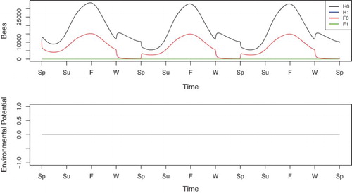
4.3. Base case simulation

We first examine a base case with no disease in the system. The simulation results are shown in Figure 1. In the absence of N. ceranae, the colony very quickly reaches a healthy periodic solution, as shown in Figure 1. Since no disease is introduced, the colony only contains healthy hive bees and healthy forager bees. The populations fluctuate with the seasons as expected. The colony population peaks towards the end of Summer and reaches a minimum near the end of Winter. Foragers return to the hive in Winter, increasing hive bee populations. This effect is reversed at the beginning of Spring.

Figure 1. Base case simulation of Equations (1(1) ${\dot{H}}_0=\beta \left(t\right)\frac{Z^n}{\kappa (t{)}^n+Z^n}-{\sigma }_1\left(t\right)H_0+{\sigma }_2\left(t\right)\frac{F}{Z}{F}_0-{\eta }_0\left(t\right)H_0-\alpha \left(t\right)H_0\frac{E}{\lambda \left(t\right)+E},$(1) )–(6(6) $H:=H_0+H_1,F:=F_0+F_1,Z:=H+F.$(6) ) without disease, $\tilde{\alpha }=0.17,{\gamma }_W=0.12$.

4.4. Simulation of a colony infected with N. ceranae

To study the effect of N. ceranae infection on the fate of a honeybee colony, we conduct simulations of the model (1(1) ${\dot{H}}_0=\beta \left(t\right)\frac{Z^n}{\kappa (t{)}^n+Z^n}-{\sigma }_1\left(t\right)H_0+{\sigma }_2\left(t\right)\frac{F}{Z}{F}_0-{\eta }_0\left(t\right)H_0-\alpha \left(t\right)H_0\frac{E}{\lambda \left(t\right)+E},$(1) )–(6(6) $H:=H_0+H_1,F:=F_0+F_1,Z:=H+F.$(6) ) varying the spore uptake rate $\tilde{\alpha }$ and the spore deposition rate γ (in terms of ${\gamma }_W$, cf. Table 1) and observing how they affect the long-term behaviour. To simulate the onset of the disease, we increase the level of $H_1$ to 10 on the first day of Winter of the first year to simulate a small number of infected individuals returning to the hive for Winter.

4.4.1. Effect of spore uptake rate $\tilde{\alpha }$ on long-term behaviour of the solution

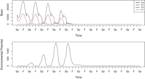
Based on exploratory tests, we first set ${\gamma }_W=0.1$ and vary $\tilde{\alpha }$ between 0.1 and 0.2, in increments of 0.005. We present in detail the simulation results for $\tilde{\alpha }=0.13$, 0.15, and 0.18, each of which leads to qualitative different long-term behaviours.

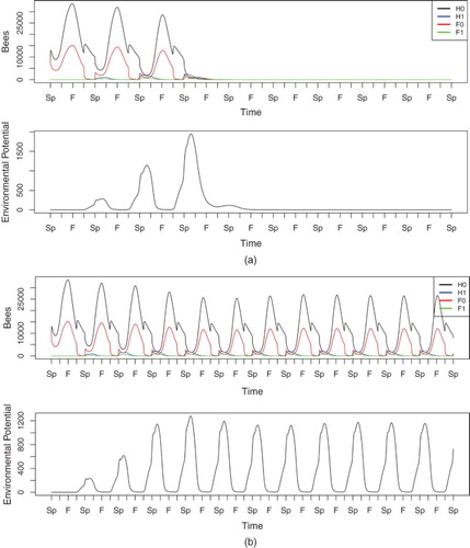
When $\tilde{\alpha }=0.13$, cf. Figure 2, the disease potential grows steadily over several years. In Spring of the second year, a small percentage of hive bees are infected, and this percentage increases in the third and fourth years as well, although the colony is able to survive with decreasing populations. In the fourth year, the infected hive bee population exceeds the healthy hive bee population slightly, and the hive is significantly weakened as it enters the following Winter. In the fifth year, the colony population plummets immediately after foragers begin to leave the hive, and the colony is effectively dead by the end of Summer. The environmental potential grows larger in each Winter initially, when the hive has sufficient numbers of bees. In the fourth Winter, the potential peaks at a slightly lower value than in the prior year, before being depleted due to natural decay following the colony's failure.

Figure 2. Simulation of Equations (1(1) ${\dot{H}}_0=\beta \left(t\right)\frac{Z^n}{\kappa (t{)}^n+Z^n}-{\sigma }_1\left(t\right)H_0+{\sigma }_2\left(t\right)\frac{F}{Z}{F}_0-{\eta }_0\left(t\right)H_0-\alpha \left(t\right)H_0\frac{E}{\lambda \left(t\right)+E},$(1) )–(6(6) $H:=H_0+H_1,F:=F_0+F_1,Z:=H+F.$(6) ) with low spore uptake rate $\tilde{\alpha }=0.13$ (${\gamma }_W=0.1$).

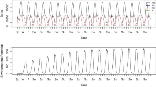
In Figure 3, the disease is reined in by a higher uptake rate of $\tilde{\alpha }=0.15$, to the extent that the hive does not die but instead reaches an endemic periodic solution. The number of infected hive bees remains low, although it is large enough to replenish the disease reservoir each year. The environmental potential increases every year until it reaches a periodic solution. In Figure 2, where the colony eventually failed, this reservoir reached approximately 1500 units at its maximum, whereas in the endemic scenario, the potential approaches roughly 350 units at its peak.

Figure 3. Simulation of Equations (1(1) ${\dot{H}}_0=\beta \left(t\right)\frac{Z^n}{\kappa (t{)}^n+Z^n}-{\sigma }_1\left(t\right)H_0+{\sigma }_2\left(t\right)\frac{F}{Z}{F}_0-{\eta }_0\left(t\right)H_0-\alpha \left(t\right)H_0\frac{E}{\lambda \left(t\right)+E},$(1) )–(6(6) $H:=H_0+H_1,F:=F_0+F_1,Z:=H+F.$(6) ) with moderate spore uptake rate $\tilde{\alpha }=0.15$ (${\gamma }_W=0.1$).

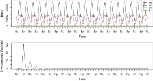
When the spore uptake rate increases more, as in Figure 4 where $\tilde{\alpha }=0.18$, the spores are eliminated quickly enough that the disease cannot take root in the hive. In this scenario, we do not see significant levels of infection, even in the first few years when the disease potential is largest. The colony eventually approaches a disease-free periodic solution. The environmental potential peaks in the first Winter at around 150 units. This is quite low in comparison to the previous simulations. Each year, the level of the reservoir peaks at a lower value until the disease is effectively eradicated.

Figure 4. Simulation of Equations (1(1) ${\dot{H}}_0=\beta \left(t\right)\frac{Z^n}{\kappa (t{)}^n+Z^n}-{\sigma }_1\left(t\right)H_0+{\sigma }_2\left(t\right)\frac{F}{Z}{F}_0-{\eta }_0\left(t\right)H_0-\alpha \left(t\right)H_0\frac{E}{\lambda \left(t\right)+E},$(1) )–(6(6) $H:=H_0+H_1,F:=F_0+F_1,Z:=H+F.$(6) ) with high spore uptake rate $\tilde{\alpha }=0.18$ (${\gamma }_W=0.1)$.

In Figure 5(a)–(c), we plot the values of $H_0$, $H_1$, and E at the beginning of Spring after a periodic solution was attained, for values of $\tilde{\alpha }$ between 0.1 and 0.2; the data for $F_0$ and $F_1$ exhibit similar behaviour to those of $H_0$ and $H_1$, respectively (data not shown). The curves for E closely resemble the ones for $H_1$, i.e. higher spore levels in the hive are directly correlated with higher numbers of infected bees. Low levels of $\tilde{\alpha }$ lead to hive failure. Moderate values of $\tilde{\alpha }$ yield endemic periodic solutions where the colony survives in the presence of the diseases. High levels remove all potential, leaving a healthy hive. We find the empty-hive solution being stable for $\tilde{\alpha }\le 0.135$, the endemic periodic solution being stable for $0.14\le \tilde{\alpha }\le 0.165$, and the healthy hive being stable for $0.17\le \tilde{\alpha }$.

Figure 5. Simulation results for disease infected colonies with varying uptake rate $\tilde{\alpha }$ and fixed deposition rate ${\gamma }_W$ [left column (a)–(c)] and varying ${\gamma }_W$ with fixed $\tilde{\alpha }$ [right column (d)–(f)]. Shown are data for the first day of Spring after a periodic solution is obtained.

It is difficult, based on the current literature, to determine exact values for $\tilde{\alpha }$ or for λ in the ecological context. Therefore, our results are qualitative in nature. We infer from these simulations a direct relationship between the spore uptake rate and the strength of the colony. We also note the possibility for all three potential outcomes: colony failure, endemic colony infection, and disease eradication.

4.4.2. Effect of spore deposition rate γ on long-term behaviour of the solution

We fix $\tilde{\alpha }=0.17$ in Spring, Summer, and Fall and $\tilde{\alpha }=0.0$ in Winter, and vary ${\gamma }_W$ from 0.1 to 0.2. We find that increasing ${\gamma }_W$ has the same qualitative effect that decreasing $\tilde{\alpha }$ had in Section 4.4.1. In Figure 5(d)–(f), we give the values of $H_0$, $H_1$, and E on the first day of Spring after a periodic solution has been reached (data for $F_0$, $F_1$ follow those for $H_0$, $H_1$ closely and are not shown). The healthy hive periodic solution is stable for ${\gamma }_W\le 0.105$. The endemic periodic solution is stable for $0.11\le {\gamma }_W\le 0.12$, where uninfected and infected bees are present, and the empty-hive periodic solution is stable for $0.125\le {\gamma }_W$, where all populations fall to zero.

Low spore deposition rates prevent the disease from taking root and maintain a disease-free colony. In these cases, the qualitative simulation looks qualitatively very similar to that in Figure 4 (data not shown). Infection levels remain low throughout all years, and the environmental potential peaks in the first year before decreasing in each subsequent year. Moderate spore deposition rates yield an endemic periodic solution in the hive. Infection levels are initially low and increase over time, although they do not grow large enough to cause colony death, cf. Figure 6(b). This does result, however, in reduced colony populations (with greater reductions than in Figure 3), which we will explore below in conjunction with other effects.

Figure 6. Simulations of Equations (1(1) ${\dot{H}}_0=\beta \left(t\right)\frac{Z^n}{\kappa (t{)}^n+Z^n}-{\sigma }_1\left(t\right)H_0+{\sigma }_2\left(t\right)\frac{F}{Z}{F}_0-{\eta }_0\left(t\right)H_0-\alpha \left(t\right)H_0\frac{E}{\lambda \left(t\right)+E},$(1) )–(5(5) $\dot{E}=\gamma \left(t\right)H_1-\delta \left(t\right)E-\tilde{\alpha }\left(t\right)H_0\frac{E}{\lambda \left(t\right)+E},$(5) ) with different spore deposition rates ${\gamma }_W$ and fixed spore uptake rate $\tilde{\alpha }=0.17$. (a) high spore deposition rate ${\gamma }_W=0.125$ and (b) moderate spore deposition rate ${\gamma }_W=0.12$.

This aligns with our analysis of the autonomous case, which suggested that high values of ${\gamma }_W$ would destabilize the disease-free limit cycle, as they required $\gamma <{\eta }_1$ in the constant coefficient case, and would lead to a stable non-trivial solution instead.

Again, we note that, in the absence of confident estimations of either parameter, the quantitative impact of these simulations should not be overstated. Instead, we focus on the qualitative implications of these results on the existence of the three limit cycles and on the relationship between these parameters and colony strength.

Also to be noted from these graphs, and from those demonstrating the effect of $\tilde{\alpha }$ on these populations, is the impact on the colony of the Allee effect imposed on the eclosion function. Rather than having the colony populations slowly decrease to an empty hive, there is a sudden drop when, above, $\tilde{\alpha }\approx 0.1325$ and ${\gamma }_W=0.1$, as well as when $\tilde{\alpha }=0.17$ and ${\gamma }_W\approx 0.1225$.

High levels of ${\gamma }_W$ overwhelm the colony and lead to colony failure, as shown in Figure 6(a) where ${\gamma }_W=0.125$. This result occurs in the Spring of the fourth year, which is earlier than the colony death seen in Figure 2. Here, the infected hive bee population overtakes that of the healthy hive bees in Spring of the fourth year, and the colony dies early in that year. In this case, we also see high levels of infected forager bees prior to colony death. Increasing ${\gamma }_W$ further only results in a faster colony death.

The environmental potential peaks in the third year around 2000 units. This quickly leads to colony failure as the infection rates increase quickly, in contrast to Figure 2, where the colony decline extended over several years.

4.5. Homing failure and Nosema infections

We investigate now the effect of Nosema combined with a second stressor, namely increased homing failure of foragers, on a colony. For example, certain pesticides have been shown to interfere with a bee's memory and navigational capacity, which can prevent a forager bee from successfully returning to the hive [18]. This can quickly lead to death for the individual bee, which cannot survive on its own. To incorporate this into our model, we follow the approach of Henry et al. [18] and augment the death rates of foraging bees. Our modified model is then (30) ${\dot{H}}_0=\beta \left(t\right)\frac{Z^n}{\kappa (t{)}^n+Z^n}-{\sigma }_1\left(t\right)H_0+{\sigma }_2\left(t\right)\frac{F}{Z}{F}_0-{\eta }_0\left(t\right)H_0-\alpha \left(t\right)H_0\frac{E}{\lambda \left(t\right)+E},$(30) (31) ${\dot{H}}_1=-{\sigma }_1\left(t\right)H_1+{\sigma }_2\left(t\right)\frac{F}{Z}{F}_1-{\eta }_1\left(t\right)H_1+\alpha \left(t\right)H_0\frac{E}{\lambda \left(t\right)+E},$(31) (32) ${\dot{F}}_0=+{\sigma }_1\left(t\right)H_0-{\sigma }_2\left(t\right)\frac{F}{Z}{F}_0-\left({\phi }_0\right(t)+\xi (t\left)\right)F_0,$(32) (33) ${\dot{F}}_1=+{\sigma }_1\left(t\right)H_1-{\sigma }_2\left(t\right)\frac{F}{Z}{F}_1-\left({\phi }_1\right(t)+\xi (t\left)\right)F_1,$(33) (34) $\dot{E}=\gamma \left(t\right)H_1-\delta \left(t\right)E-\tilde{\alpha }\left(t\right)H_0\frac{E}{\lambda +E},$(34) where $\xi \left(t\right)$ is the increase (due to homing failure) in forager deaths. We include these increases in forager loss rate for a 21-day period at the beginning of Spring in Years 4 through 6, mimicking the spray application of neonicotinoid pesticides on crops near the colony. We first run simulations with low, medium, and high homing failure rates of (a) 0.102, (b) 0.209, and (c) 0.316, respectively [18], without Nosema infection, and compare these to the case without homing failure as shown in Figure 1. The results of these simulations are plotted in Figure 7.

Figure 7. Simulation of model (30(30) ${\dot{H}}_0=\beta \left(t\right)\frac{Z^n}{\kappa (t{)}^n+Z^n}-{\sigma }_1\left(t\right)H_0+{\sigma }_2\left(t\right)\frac{F}{Z}{F}_0-{\eta }_0\left(t\right)H_0-\alpha \left(t\right)H_0\frac{E}{\lambda \left(t\right)+E},$(30) )–(34(34) $\dot{E}=\gamma \left(t\right)H_1-\delta \left(t\right)E-\tilde{\alpha }\left(t\right)H_0\frac{E}{\lambda +E},$(34) ) for two different homing failure rates without Nosema. (a) low level of homing failure, $\xi =0.102$ and (b) medium level of homing failure, $\xi =0.209$.

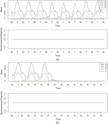
In Figure 7(a), the colony population size drops during the weeks of low additional homing failure $\xi =0.102$. The colony is able to survive this added stress. After increased homing failure applications end, the colony quickly returns in the following year to its previous strength.

For moderate homing failure, $\xi =0.209$, Figure 7(b) shows that the colony quickly dies in Spring of the fourth year, despite having appeared healthy up until this point. The heightened forager death rate draws hive bees out at a faster rate, and the colony is unable to sustain itself through newly emerging bees, which leads to hive failure. Given that this moderate level can already wipe out a colony, we omit results for a high level of homing failure (data not shown).

Finally, we combine increased homing failure and nosemosis. We use the lower homing failure rate of $\xi =0.102$. For infection parameters, we take ${\gamma }_W=0.12$ and $\tilde{\alpha }=0.17$, which, as shown in Figure 6(b), will (in the absence of homing failure) result in an endemic periodic solution with a small reduction in colony size. This periodic solution is reached after 13 years, so we first allow the system to approach periodicity and then apply increased homing failure rates in years 13, 14, and 15.

The results of this simulation are shown in Figure 8. The colony, after initial innoculation, survives several seasons of infection. While infected bees are present, their population remains relatively low, and the environmental potential stays well below the level at which mass outbreaks and/or hive failure occur. When homing failure rates increase, the increased death toll for foragers draws higher numbers of hive bees out precociously, and the colony cannot sustain itself through new births. Populations plummet and the colony dies due to the joint effect of N. ceranae and increased homing failure.

Figure 8. Simulation of colony with mild Nosema infection that is exposed to a low level increase in forager homing failure, $\xi =0.102$, ${\gamma }_W=0.12$, and $\tilde{\alpha }=0.17$.

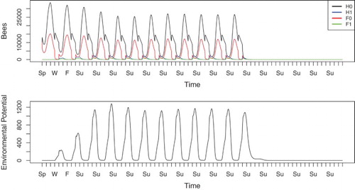
In summary, while a colony might be able to survive each individual stressor, their combined effect can be too strong and lead to colony failure.

4.6. Hive cleaning by comb replacement

Since the spores of the disease rest on the combs of the hive, some beekeepers replace a fraction of the comb frames with spore-free frames in an attempt to mitigate the infection. To investigate this with our model, we make certain assumptions about frame replacement:

1. Based on discussions with biologists and apiarists, we assume that frames can be replaced at two points of the year: in early Spring before brood combs are used to rear bees, and in late Spring when one hive maybe split into two and new combs can be placed into the split hive. We do not include hive splitting in our model but we investigate the remedial potential of frame replacement at this time of inspection.

2. We assume that frame replacement can be done instantaneously

3. Apiarists usually replace two to three of the 10 frames in a hive. With equal distribution of spores among frames, this would remove around 20–30$\mathrm{\%}$ of the environmental potential. Since distribution may be uneven, we allow for the percentage of spores removed to vary between $0\mathrm{\%}$ and $98\mathrm{\%}$ in our simulations. However, we keep this rate constant in each simulation to see the overall effect of average cleaning levels being more thorough or less thorough.

In our model, we implement this by adding a removal term, $-C\left(t\right)E$, to the equation for $\dot{E}$. $\begin{array}{rl}{\dot{H}}_0& =\beta \left(t\right)\frac{Z^n}{\kappa (t{)}^n+Z^n}-{\sigma }_1\left(t\right)H_0+{\sigma }_2\left(t\right)\frac{F}{Z}{F}_0-{\eta }_0\left(t\right)H_0-\alpha \left(t\right)H_0\frac{E}{\lambda \left(t\right)+E},\\ {\dot{H}}_1& =-{\sigma }_1\left(t\right)H_1+{\sigma }_2\left(t\right)\frac{F}{Z}{F}_1-{\eta }_1\left(t\right)H_1+\alpha \left(t\right)H_0\frac{E}{\lambda \left(t\right)+E},\\ {\dot{F}}_0& =+{\sigma }_1\left(t\right)H_0-{\sigma }_2\left(t\right)\frac{F}{Z}{F}_0-{\phi }_0\left(t\right)F_0,\\ {\dot{F}}_1& =+{\sigma }_1\left(t\right)H_1-{\sigma }_2\left(t\right)\frac{F}{Z}{F}_1-{\phi }_1\left(t\right)F_1,\\ \dot{E}& =\gamma \left(t\right)H_1-\delta \left(t\right)E-C\left(t\right)E-\tilde{\alpha }\left(t\right)H_0\frac{E}{\lambda +E}.\end{array}$

$C\left(t\right)$ is a step function which is zero at all times other than in short intervals specified for cleaning. Unlike with our other parameters, this function is not smoothened. To derive values for $C\left(t\right)$, we use a similar approach to that used to estimate values for δ in Section 4.2. We specify r, the percentage of spores to remain after cleaning, and then calculate $C\left(t_{clean}\right)=-\log \left(r\right)/\mathrm{\Delta }t$, where $t_{clean}$ is any time at which cleaning occurs, and $\mathrm{\Delta }t$ the length of the (small time interval) in which removal is applied.

Based on our simulations in Section 4.4, we select $\tilde{\alpha }=0.17$ and ${\gamma }_W=0.12$ for our disease parameters, i.e. within the range where the hive tends towards an endemic (but noticeably weakened) periodic solution in the absence of remedial action. We vary r from 0.02 to 1.0 and integrate the model in each simulation until convergence to a periodic solution.

We hypothesize that more frequent cleaning will better contain the disease, and that comb replacement is most effective when done earlier in the year. Early comb replacement should remove spores before they are able to infect the hive and propagate. To examine this, we run three experiments:

1. one in which we clean the hive on the 7th and 84th days of Spring,

2. one in which we clean only on the 7th day of Spring, and

3. one in which we clean only on the 84th day of Spring.

Figure 9(a)–(c) shows for all three scenarios the percent shortfall of the colony's population at the end of Summer as a function of the percentage of the disease reservoir removed in each instance of cleaning, r.

Figure 9. Effect of frame replacement on colony size shortfall [($\tilde{\alpha }=0.17$, ${\gamma }_W=0.12$ in all simulations]: (a) replacement on days 7 and 84, (b) on day 7, (c) on day 84, (d) on days 7 and 84 with increased homing failure in years 13–15, $\xi =0.102$.

In case (a), Figure 9(a), the colony shortfall decreases with increasing r in an sublinear fashion from roughly $21\mathrm{\%}$ to roughly $2\mathrm{\%}$. While the largest decreases in colony losses are likely unattainable, these results do suggest that comb replacement can be an efficient strategy to control Nosema. On a more practical note, if we assume that a beekeeper, by changing 2–3 frames per cleaning, can remove 20–30$\mathrm{\%}$ of the environmental potential, the colony losses can still be roughly halved, a reduction that is not insignificant.

Figure 9(b) shows for case (b) the results of the second experiment, where frames are replaced only on the 7th day of each year. Here we see less of an impact than the previous experiment: colony losses can theoretically be reduced from $20\mathrm{\%}$ of the colony to around $4\mathrm{\%}$, but a realistic approach would likely see them reduced to around $14\mathrm{\%}$. This suggests that the frequency with which one cleans has a notable effect on the containment of the disease.

In Figure 9(c), we see the impact of only replacing frames in late Spring. Under the strongest cleaning regimen, colony losses are reduced to around $7.5\mathrm{\%}$, and in the 20–30$\mathrm{\%}$ range of spore removal, they are only reduced to around $15\mathrm{\%}$. Both of these levels are higher than those seen in the second experiment, lending credence to our hypothesis that earlier cleaning is more effective. However, the actual benefit of cleaning earlier appears relatively small at lower cleaning levels.

Ultimately, we infer from these results that hive cleaning can be used to decrease colony losses at low cost to an apiary, although it is unlikely to cure a hive. It appears most effective when done often during times of high N. ceranae levels, such as in early Spring.

In light of the results from our simulation experiments involving homing failure, we investigate whether periodic comb replacement can be used to strengthen an infected colony to the point that it overcomes a bout of homing failure. To this end, we repeat the simulation of case (a) above but also consider a low increase in homing failure ($\xi =0.102$) during the first 21 days of years 13, 14, and 15. The results are presented in Figure 9(d). The colony dies in most comb replacement applications, exhibited by a $100\mathrm{\%}$ colony loss. We observe that for disease removal levels upwards of $90\mathrm{\%}$, the colony is able to survive the application of homing failure, though it still experiences a small population reduction. To clean to this extent on a regular basis is largely unattainable in reality, making frame replacement a poor response in this case. However, we note that these results would likely vary depending on the virulence of the disease (controlled by ${\gamma }_W$, $\tilde{\alpha }$, and λ), the length of the homing failure period, and the rate at which it affects bees.

5. Conclusion

The microsporidian N. ceranae is a common infectious disease of the Western honey bee that has been implicated in colony losses. It is generally acquired by worker bees that engage in comb cleaning in the hive, but it expresses itself primarily after infected workers become foragers in form of a reduced life span. In a mathematical model that describes this disease, therefore, the worker bee population is compartmentalized vertically into hive and forager bees, and horizontally into susceptible and infected individuals. Furthermore, the transmission of the disease via deposition and uptake of spores in the hive requires us to introduce an environmental reservoir of spores, rather than applying direct mass action transmission between infected and susceptible individuals as in traditional SIR models.

This prompted two major conceptual extensions of an existing simple hive–forager population model. Moreover, since the disease and its viability and infectivity level change drastically over the year, a non-autonomous system with periodic coefficients needs to be considered. The resulting model is algebraically too complex to allow for insightful rigorous mathematical analysis via Floquet theory or other standard ODE approaches. Therefore, the dynamical behaviour of the model must be studied numerically in computer simulations.

The data on Nosema currently available in the literature do not allow a full parameterization of the model. Therefore, a computational exploration must take the form of a sensitivity analysis. By focusing on only two parameters, the spore deposition rate and the spore uptake rate, we could show that, depending on parameters, several long-term outcomes are possible: (i) a disease-free hive, in which Nosema is eliminated from the hive, (ii) an endemic hive, in which the disease is present, but the colony continues to function, though at reduced strength compared to a colony without disease, and (iii) failure of the hive if the disease takes over and leads to premature loss of too many foragers for the hive to sustain itself.

We have investigated the interplay of Nosema infections and increased forager losses caused by a second stressor, such as exposure to agricultural pesticides. Even if the infection levels are low enough for the colony to survive in the absence of the second factor, or in the case of low enough forager losses for a disease-free colony to survive, we have seen that the combination of both effects can lead to the failure of the colony. This suggests that several factors combined, each of which on its own non-critical, can tip the balance in a colony and drive it to extinction. This supports the notion that colony collapse disorder or overwintering losses that have been observed in the last decade are indeed a multi-factorial problem with not a single culprit responsible.

Finally, a remedial strategy that helps to mitigate the detrimental effects of one stressor (Nosema in our case) might be insufficient if the colony is exposed to a second stressor, even at levels that are tolerable in the absence of the first one.

Disclosure statement

No potential conflict of interest was reported by the authors.

Additional information

Funding

This study was supported in part by the Ontario Ministry for Agriculture Food and Rural Affairs with a research grant (grant number SR9279) awarded to HJE under the New Directions program. AP was also supported by an Ontario Graduate Scholarship.

Appendix. Comparison of two forager recruitment terms

We compare here qualitatively and quantitatively the modified forager–hive bee transition term that we use in Equation (1(1) ${\dot{H}}_0=\beta \left(t\right)\frac{Z^n}{\kappa (t{)}^n+Z^n}-{\sigma }_1\left(t\right)H_0+{\sigma }_2\left(t\right)\frac{F}{Z}{F}_0-{\eta }_0\left(t\right)H_0-\alpha \left(t\right)H_0\frac{E}{\lambda \left(t\right)+E},$(1) )–(6(6) $H:=H_0+H_1,F:=F_0+F_1,Z:=H+F.$(6) ) with the term used in the original hive–forager model in [25]. For this comparison we consider, as in [25], the constant coefficient case with Holling Type-II eclosion rate (i.e. Hill exponent n=1).

We recall, without proof, from [25], the following result about the existence of an asymptotically stable positive equilibrium, which describes a condition for the colony to survive.

Proposition A.1

The model (A1) $\begin{array}{rl}\dot{H}& =\beta \frac{H+F}{\kappa +H+F}-{\sigma }_{1}H+{\sigma }_2\frac{F}{H+F}H,\\ \dot{F}& ={\sigma }_{1}H-{\sigma }_2\frac{F}{H+F}H-\phi F\end{array}$(A1) with positive constant parameters such that (A2) $0<\phi \left({\sigma }_1-\frac{\beta }{\kappa }\right)<\frac{\beta }{2\kappa }\left({\sigma }_1+{\sigma }_2+\sqrt{({\sigma }_1-{\sigma }_2{)}^2+4\frac{\beta {\sigma }_2}{\kappa }}\right)$(A2) has a positive asymptotically stable equilibrium $F^{\ast }=\frac{\beta }{\phi }-\frac{\kappa J}{J+1},H^{\ast }=\frac{1}{J}{F}^{\ast }$ with $J=\frac{1}{2}\left[\left(\frac{{\sigma }_1}{\phi }-\frac{{\sigma }_2}{\phi }-1\right)+\sqrt{{\left(\frac{{\sigma }_1}{\phi }-\frac{{\sigma }_2}{\phi }-1\right)}^2+4\frac{{\sigma }_1}{\phi }}\right].$

The corresponding result for the modified transition term is

Proposition A.2

The modified model (A3) $\begin{array}{rl}\dot{H}& =\beta \frac{H+F}{\kappa +H+F}-{\sigma }_{1}H+{\sigma }_2\frac{F}{H+F}F,\\ \dot{F}& ={\sigma }_{1}H-{\sigma }_2\frac{F}{H+F}F-\phi F\end{array}$(A3) with positive constant parameters such that (A4) $0<\phi \left({\sigma }_1-\frac{\beta }{\kappa }\right)<\frac{\beta }{2\kappa }\left({\sigma }_1+\sqrt{{\sigma }_1^2+4{\sigma }_2\left({\sigma }_1-\frac{\beta }{\kappa }\right)}\right)$(A4) has a positive, asymptotically stable equilibrium $F^{\ast }=\frac{\beta }{\phi }-\frac{\kappa J}{J+1},H^{\ast }=\frac{1}{J}{F}^{\ast }$ with $J=\frac{{\sigma }_1-\phi +\sqrt{({\sigma }_1+\phi {)}^2+4{\sigma }_1{\sigma }_2}}{2({\sigma }_2+\phi )}.$

Proof.

Setting the second equation in (A3(A3) $\begin{array}{rl}\dot{H}& =\beta \frac{H+F}{\kappa +H+F}-{\sigma }_{1}H+{\sigma }_2\frac{F}{H+F}F,\\ \dot{F}& ={\sigma }_{1}H-{\sigma }_2\frac{F}{H+F}F-\phi F\end{array}$(A3) ) to zero and multiplying out the fractional part gives the quadratic equation $0=-({\sigma }_2+\phi )F^{\ast 2}+({\sigma }_1-\phi )H^{\ast }{F}^{\ast }+{\sigma }_1{H}^{\ast 2}.$ Solving this for $F^{\ast }$ we find the relationship between $F^{\ast }$ and $H^{\ast }$ (A5) $F^{\ast }=J{H}^{\ast },$(A5) where (A6) $J=\frac{{\sigma }_1-\phi \pm \sqrt{({\sigma }_1+\phi {)}^2+4{\sigma }_1{\sigma }_2}}{2({\sigma }_2+\phi )}.$(A6) Positivity of the equilibrium requires that J>0, i.e. that the positive branch is chosen. Setting the first equation in (A3(A3) $\begin{array}{rl}\dot{H}& =\beta \frac{H+F}{\kappa +H+F}-{\sigma }_{1}H+{\sigma }_2\frac{F}{H+F}F,\\ \dot{F}& ={\sigma }_{1}H-{\sigma }_2\frac{F}{H+F}F-\phi F\end{array}$(A3) ) to zero and using (A5(A5) $F^{\ast }=J{H}^{\ast },$(A5) ), we find the equilibrium $H^{\ast }=\frac{\beta }{\phi J}-\frac{\kappa }{J+1},F^{\ast }=\frac{\beta }{\phi }-\frac{\kappa J}{J+1}.$ To assess the stability of this equilibrium, we consider the Jacobian $\mathcal{J}(H^{\ast },F^{\ast })=\left(\begin{array}{cc}\frac{{\phi }^2{J}^2\kappa }{\beta (J+1{)}^2}-{\sigma }_1-{\sigma }_2\frac{J^2}{(J+1{)}^2}& \frac{{\phi }^2{J}^2\kappa }{\beta (J+1{)}^2}+{\sigma }_2\frac{J(J+2)}{(J+1{)}^2}\\ {\sigma }_1+{\sigma }_2\frac{J^2}{(J+1{)}^2}& -{\sigma }_2\frac{J(J+2)}{(J+1{)}^2}-\phi \end{array}\right).$ For asymptotic stability we require the determinant of this matrix to be positive and its trace to be negative. From Equation (A6(A6) $J=\frac{{\sigma }_1-\phi \pm \sqrt{({\sigma }_1+\phi {)}^2+4{\sigma }_1{\sigma }_2}}{2({\sigma }_2+\phi )}.$(A6) ), we find after re-arranging ${\sigma }_1={\sigma }_2{J}^2/(J+1)+\phi J$, which allows to simplify the condition on the determinant to (A7) $\frac{\beta }{\kappa }>\frac{\phi J}{J+1}.$(A7) If this condition is satisfied, then the negativity condition on the trace becomes, after some minor steps $0<\frac{\phi (J^2+J+1)+{\sigma }_{2}J(J+2)}{J+1},$ which is trivially satisfied for J>0.

We can simplify Equation (A7(A7) $\frac{\beta }{\kappa }>\frac{\phi J}{J+1}.$(A7) ) to eliminate J. Substituting Equation (A6(A6) $J=\frac{{\sigma }_1-\phi \pm \sqrt{({\sigma }_1+\phi {)}^2+4{\sigma }_1{\sigma }_2}}{2({\sigma }_2+\phi )}.$(A6) ), we get (A8) $\frac{\kappa \phi }{\beta }({\sigma }_1-\phi +\sqrt{({\sigma }_1+\phi {)}^2+4{\sigma }_1{\sigma }_2})<{\sigma }_1+\phi +2{\sigma }_2+\sqrt{({\sigma }_1+\phi {)}^2+4{\sigma }_1{\sigma }_2}.$(A8) We reformulate this as an inequality condition on φ in terms of the other model parameters. After some calculations to simplify the expressions, we find that φ must be bounded from above by the positive root of the quadratic polynomial $(\kappa {\sigma }_1-\beta ){\hat{\phi }}^2-{\sigma }_1\beta \hat{\phi }-\frac{{\sigma }_2{\beta }^2}{\kappa }=0.$ For such a positive root to exist we require ${\sigma }_1>\beta /\kappa$. Under this condition, we find $0<\phi <\frac{\beta }{2}\left[\frac{{\sigma }_1\pm \sqrt{{\sigma }_1^2+4{\sigma }_2({\sigma }_1-\frac{\beta }{\kappa })}}{\kappa {\sigma }_1-\beta }\right]=\hat{\phi }.$ From this follows Equation (A4(A4) $0<\phi \left({\sigma }_1-\frac{\beta }{\kappa }\right)<\frac{\beta }{2\kappa }\left({\sigma }_1+\sqrt{{\sigma }_1^2+4{\sigma }_2\left({\sigma }_1-\frac{\beta }{\kappa }\right)}\right)$(A4) ).

Note that the first inequality condition ${\sigma }_1>\beta /\kappa$ is the same for both models in Equations (A2(A2) $0<\phi \left({\sigma }_1-\frac{\beta }{\kappa }\right)<\frac{\beta }{2\kappa }\left({\sigma }_1+{\sigma }_2+\sqrt{({\sigma }_1-{\sigma }_2{)}^2+4\frac{\beta {\sigma }_2}{\kappa }}\right)$(A2) ) and (A4(A4) $0<\phi \left({\sigma }_1-\frac{\beta }{\kappa }\right)<\frac{\beta }{2\kappa }\left({\sigma }_1+\sqrt{{\sigma }_1^2+4{\sigma }_2\left({\sigma }_1-\frac{\beta }{\kappa }\right)}\right)$(A4) ). For given maximum eclosion rate β, it sets a lower bound on the nominal hive–forager transition rate, whereas in both cases the second inequality sets an upper bound on the forager mortality rate φ that can be tolerated. This upper bound depends in both cases on the maximum reversion rate ${\sigma }_2$. The exact form of this dependence is different for both models, but in both cases, sufficiently large ${\sigma }_2$ suffice.

Phase portraits for both models are shown in Figure A1, for the original parameters in [25]: $\beta =2000$, $\kappa =27,000$, ${\sigma }_1=0.25$, and $\phi =0.24$. The one exception we make is for ${\sigma }_2$, which we set at 0.75 for the original model and at 1.5 for the modified term, to maintain the forager–hive bee ratio.

Figure A.1. Phase portraits of autonomous hive–forager models: (a) system (A1(A1) $\begin{array}{rl}\dot{H}& =\beta \frac{H+F}{\kappa +H+F}-{\sigma }_{1}H+{\sigma }_2\frac{F}{H+F}H,\\ \dot{F}& ={\sigma }_{1}H-{\sigma }_2\frac{F}{H+F}H-\phi F\end{array}$(A1) ) with the terms of [25] and parameters satisfying the stability condition (A2(A2) $0<\phi \left({\sigma }_1-\frac{\beta }{\kappa }\right)<\frac{\beta }{2\kappa }\left({\sigma }_1+{\sigma }_2+\sqrt{({\sigma }_1-{\sigma }_2{)}^2+4\frac{\beta {\sigma }_2}{\kappa }}\right)$(A2) ); (b) system (A3(A3) $\begin{array}{rl}\dot{H}& =\beta \frac{H+F}{\kappa +H+F}-{\sigma }_{1}H+{\sigma }_2\frac{F}{H+F}F,\\ \dot{F}& ={\sigma }_{1}H-{\sigma }_2\frac{F}{H+F}F-\phi F\end{array}$(A3) ) with the modified terms and parameters satisfying the stability condition (A4(A4) $0<\phi \left({\sigma }_1-\frac{\beta }{\kappa }\right)<\frac{\beta }{2\kappa }\left({\sigma }_1+\sqrt{{\sigma }_1^2+4{\sigma }_2\left({\sigma }_1-\frac{\beta }{\kappa }\right)}\right)$(A4) ).

While the two models are not quantitatively identical, their qualitative similarities are strong enough to support the statement that the modification of the model prompted by necessity in the case of a Nosema infection does not qualitatively alter the model in the disease-free case that was studied in [25].

References

- M.D. Allen and E.P. Jeffree, The influence of stored pollen and of colony size on the brood rearing of honeybees, Ann. Appl. Biol. 44(4) (1956), pp. 649–656. doi: 10.1111/j.1744-7348.1956.tb02164.x
- L. Bailey, Honey bee pathology, Ann. Rev. Entomol. 13(1) (1968), pp. 191–212. doi: 10.1146/annurev.en.13.010168.001203
- F. Becerra-Guzmán, E. Guzmán-Novoa, A. Correa-Benítez, and A. Zozaya-Rubio, Length of life, age at first foraging and foraging life of Africanized and European honey bee (Apis mellifera) workers, during conditions of resource abundance, J. Apicult. Res. 44(4) (2005), pp. 151–156. doi: 10.1080/00218839.2005.11101170
- M.A. Becher, J.L. Osborne, P. Thorbek, P.J. Kennedy, V. Grimm, and I. Steffan-Dewenter, REVIEW: Towards a systems approach for understanding honeybee decline: A stocktaking and synthesis of existing models, J. Appl. Ecol. 50(4) (2013), pp. 868–880. doi: 10.1111/1365-2664.12112
- S.N. Beshers, Z.Y. Huang, Y. Oono, and G.E. Robinson, Social inhibition and the regulation of temporal polyethism in honey bees, J. Theor. Biol. 213(3) (2001), pp. 461–479. doi: 10.1006/jtbi.2001.2427
- M.I. Betti, L.M. Wahl, M. Zamir, and O. Rueppell, Effects of infection on honey bee population dynamics: A model, PloS One 9(10) (2014), p. e110237. doi: 10.1371/journal.pone.0110237
- H.W. Borchers, pracma: Practical numerical math functions, R package version 1.8.8, 2015; available at http://CRAN.R-project.org/package=pracma, 2015.
- R. Brodschneider and K. Crailsheim, Nutrition and health in honey bees, Apidol. 41(3) (2010), pp. 278–294. doi: 10.1051/apido/2010012
- J. Bryden, R.J. Gill, R.A.A. Mitton, N.E. Raine, V.A. A. Jansen, and D. Hodgson, Chronic sublethal stress causes bee colony failure, Ecol. Lett. 16(12) (2013), pp. 1463–1469. doi: 10.1111/ele.12188
- Y. Chen, J.D. Evans, I.B. Smith, and J.S. Pettis, Nosema ceranae is a long-present and wide-spread microsporidian infection of the European honey bee (Apis mellifera) in the United States, J. Inverteb. Pathol. 97(2) (2008), pp. 186–188. doi: 10.1016/j.jip.2007.07.010
- H.J. Eberl, M. Frederick, and P. Kevan, The importance of brood maintenance terms in simple models of the honeybee ‘Varroa destructor’ acute bee paralysis virus complex, Electron. J. Differ. Eq. CS19 (2010), pp. 85–98.
- B. Emsen, E. Guzman-Novoa, M.M. Hamiduzzaman, L. Eccles, B. Lacey, R.A. Ruiz-Pérez, and M. Nasr, Higher prevalence and levels of Nosema ceranae than Nosema apis infections in Canadian honey bee colonies, Parasitol. Res. 115(1) (2016), pp. 175–181. doi: 10.1007/s00436-015-4733-3
- D. van Engelsdorp, J. Hayes Jr., R.M. Underwood, and J.S. Pettis, A survey of honey bee colony losses in the United States, Fall 2008 to Spring 2009, J. Apicult. Res. 49(1) (2010), pp. 7–14. doi: 10.3896/IBRA.1.49.1.03
- E. Forsgren and I. Fries, Comparative virulence of Nosema ceranae and Nosema apis in individual European honey bees, Vet. Parasitol. 170(3) (2010), pp. 212–217. doi: 10.1016/j.vetpar.2010.02.010
- M. Goblirsch, Z.Y. Huang, M. Spivak, and G.V. Amdam, Physiological and behavioral changes in honey bees (Apis mellifera) induced by Nosema ceranae infection, PLoS One 8(3) (2013), p. e58165. doi: 10.1371/journal.pone.0058165
- Government of Canada, Canadian Climate Normals 1981–2010 Station Data. Available at http://climate.weather.gc.ca/climate_normals, Accessed 15 January 2016.
- P. Graystock, D. Goulson, and W.H.O. Hughes, Parasites in bloom: Flowers aid dispersal and transmission of pollinator parasites within and between bee species, Proc. R. Soc. B 282 (2015), p. 20151371. doi: 10.1098/rspb.2015.1371
- M. Henry, M. Beguin, F. Requier, O. Rollin, J.-F. Odoux, P. Aupinel, J. Aptel, S. Tchamitchian, and A. Decourtye, A common pesticide decreases foraging success and survival in honey bees, Science 336(6079) (2012), pp. 348–350. doi: 10.1126/science.1215039
- M. Higes, R. Martín-Hernández, C. Botías, E.G. Bailón, A.V. González-Porto, L. Barrios, M.J. del Nozal, J.L. Bernal,J.J. Jiménez, P.G. Palencia, and A. Meana, How natural infection by Nosema ceranae causes honeybee colony collapse, Environ. Microbiol. 10(10) (2008), pp. 2659–2669. doi: 10.1111/j.1462-2920.2008.01687.x
- M. Higes, R. Martín-Hernández, E. Garrido-Bailón, P. García-Palencia, and A. Meana, Detection of infective Nosema ceranae (Microsporidia) spores in corbicular pollen of forager honeybees, J. Invertebr. Pathol. 97 (2008), pp. 76–78. doi: 10.1016/j.jip.2007.06.002
- M. Higes, A. Meana, C. Bartolomé, C. Botías, and R. Martín-Hernández, Nosema ceranae (Microsporidia), a controversial 21st century honey bee pathogen, Env. Microbiol. Reports 5(1) (2013), pp. 17–29. doi: 10.1111/1758-2229.12024
- L. Hogben, Handbook of Linear Algebra, CRC Press, Boca Raton, FL, 2006.
- W.-F. Huang, L. Solter, K. Aronstein, and Z. Huang, Infectivity and virulence of Nosema ceranae and Nosema apis in commercially available North American honey bees, J. Inverteb. Pathol. 124 (2015), pp. 107–113. doi: 10.1016/j.jip.2014.10.006
- P.G. Kevan, E. Guzman, A. Skinner, and D. van Englesdorp, Colony collapse disorder in Canada: do we have a problem? Hive Lights 20(4) (2007), pp. 14–16.
- D.S. Khoury, M.R. Myerscough, A.B. Barron, and J.A.R. Marshall, A quantitative model of honey bee colony population dynamics, PloS One 6(4) (2011), p. e18491. doi: 10.1371/journal.pone.0018491
- D.S. Khoury, A.B. Barron, M.R. Myerscough, and A.G. Dyer, Modelling food and population dynamics in honey bee colonies, PloS One 8(5) (2013), p. e59084. doi: 10.1371/journal.pone.0059084
- C.M. Kribs-Zaleta and C. Mitchell, Modeling colony collapse disorder in honeybees as a contagion, Math. Biosc. Eng. 11(6) (2014), pp. 1275–1294. doi: 10.3934/mbe.2014.11.1275
- B. Lacey, A two year study of Nosema ceranae in Ontario, Ontario Bee J. 33(2) (2014), pp. 14–16.
- A.R. McLellan, Growth and decline of honeybee colonies and inter-relationships of adult bees, brood, honey and pollen, J. Appl. Ecol. 15 (1978), pp. 155–161. doi: 10.2307/2402927
- F.E. Moeller, Nosema Disease: Its Control in Honey Bee Colonies, USDA Science and Education Administration, Vol. 1569, 1978.
- National Research Council (US). Committee on the Status of Pollinators in North America and National Academies Press (US), Status of Pollinators in North America, Natl. Academy Pr, 2007.
- S.G. Potts, S.P.M. Roberts, R. Dean, G. Marris, M.A. Brown, R. Jones, P. Neumann, and J. Settele, Declines of managed honey bees and beekeepers in Europe, J. Apicult. Res. 49(1) (2010), pp. 15–22. doi: 10.3896/IBRA.1.49.1.02
- V. Ratti, P.G. Kevan, and H.J. Eberl, A mathematical model of the honeybee–varroa destructor–acute bee paralysis virus system with seasonal effects, Bull. Math. Biol. 77(8) (2015), pp. 1493–1520. doi: 10.1007/s11538-015-0093-5
- S.F. Sakagami and H. Fukuda, Life tables for worker honeybees, Res. Pop. Ecol. 10(2) (1968), pp. 127–139. doi: 10.1007/BF02510869
- T.D. Seeley, Honeybee Ecology: A Study of Adaptation in Social Life, Princeton University Press, Princeton, NJ, 1985.
- T.D. Seeley, The Wisdom of the Hive: The Social Physiology of Honey Bee Colonies, Harvard University Press, Cambridge, MA, 2009.
- K. Soetaert, T. Petzoldt, and R.W. Setzer, Solving differential equations in R: package deSolve, J. Stat. Softw. 33(9) (2010), pp. 1–25. doi: 10.18637/jss.v033.i09
- M. Spivak, E. Mader, M. Vaughan, N.H. Euliss Jr., and H. Ned, The plight of the bees, Environ. Sci. Tech. 45(1) (2010), pp. 34–38. doi: 10.1021/es101468w
- D.J.T. Sumpter and S.J. Martin, The dynamics of virus epidemics in varroa-infested honey bee colonies, J. Animal Ecol. 73(1) (2004), pp. 51–63. doi: 10.1111/j.1365-2656.2004.00776.x
- C. Thom, T.D. Seeley, and J. Tautz, A scientific note on the dynamics of labor devoted to nectar foraging in a honey bee colony: Number of foragers versus individual foraging activity, Apidol. 31(6) (2000), pp. 737–738. doi: 10.1051/apido:2000158
- W. Walter, Ordinary Differential Equations, Springer, New York, 1998.
- G.R. Williams, M.A. Sampson, D. Shutler, and R.E.L. Rogers, Does fumagillin control the recently detected invasive parasite Nosema ceranae in western honey bees (Apis mellifera)? J. Invertebr. Pathol. 99(3) (2008), pp. 342–344. doi: 10.1016/j.jip.2008.04.005
- M.L. Winston, The Biology of the Honey Bee, Harvard University Press, Cambridge, MA, 1991.