The transmission dynamic and optimal control of acute and chronic hepatitis B

ABSTRACT

In this article, we present the transmission dynamic of the acute and chronic hepatitis B epidemic problem and develop an optimal control strategy to control the spread of hepatitis B in a community. In order to do this, first we present the model formulation and find the basic reproduction number $R_0$. We show that if $R_0\le 1,$ then the disease-free equilibrium is both locally as well as globally asymptotically stable. Then, we prove that the model is locally and globally asymptotically stable, if $R_0>1$. To control the spread of this infection, we develop a control strategy by applying three control variables such as isolation of infected and non-infected individuals, treatment and vaccination to minimize the number of acute infected, chronically infected with hepatitis B individuals and maximize the number of susceptible and recovered individuals. Finally, we present numerical simulation to illustrate the feasibility of the control strategy.

KEYWORDS:

• Epidemic model
• basic reproduction number
• stability analysis
• optimal control strategy
• numerical simulation

AMS SUBJECT CLASSIFICATION:

• 92D25
• 49J15
• 93D20

1. Introduction

The most important organ in the human body is the liver. Liver infection causes different diseases. Hepatitis B is one of the contagious diseases causing inflammation of the liver. The virus itself does not cause direct damage to the liver cell, but the response of the immune system leads to the inflammation of liver. When hepatitis B virus (HBV) enter the body, it infects the cells in the liver, which are called hepatocytes. As a result the immune system targets hepatocyte and produces inflammation of the liver [4]. Infection of hepatitis B has two phases, acute hepatitis and chronic hepatitis. Acute hepatitis B refers to the first six months of exposure of the patients's body to HBV. In this stage the immune system is usually able to clear the virus from the body and the individual may completely recover within a few months. Chronic hepatitis B refers to the illness that occurs when HBV remains in the body for a long time and develops serious health problem. Individuals with chronic hepatitis often do have no history of acute illness, but it can cause liver scarring that causes liver failure and may also develop liver cancer [13].

HBV can be transmitted from one individual to another individual on different ways, such as transmission of blood, semen and vaginal secretions [10,12,15]. Another major transmission of HBV is the unprotected sexual contact, sharing of razors, blades or tooth brushes [3]. Also the virus transmits from an infected mother to her child during the time of birth. However, HBV cannot be transmitted through water, food, hugging, kissing and causal contact such as in the work place, school, etc. [15]. The mode of transmission of HBV and HIV is the same, but HBV is 50–100 times more infectious [20].

HBV infection is a global health problem. According to WHO about 400 million population is infected world wide chronically. In China 93 million population are affected due to HBV infections [11,23]. Vaccine for the prevention of hepatitis B is available in the market that is very effective [14,19].

In the real world phenomena mathematical modelling is one of the powerful tools to describe the dynamical behaviour of different diseases [21,22,24,25]. Mathematicians and biologists used different epidemic models to understand the transition of different infectious diseases in the population. In 1991 Anderson and May described the effect of carriers on transmission of HBV by using a simple deterministic model [1]. Nokes et al. [17] presented a model for the transmission dynamic of hepatitis B. Medley et al. used a mathematical model for eliminating HBV in New Zealand  [16]. Zhao et al. presented an age-structured model for the prediction of HBV transmission and evaluated the long-term effectiveness of the vaccination programme in China [27]. Dontwi et al. [5] studied a transmission model for HBV. Khan and Zaman developed an epidemic model for the transmission dynamic and vaccination of hepatitis B [8].

In this article, we develop a HBV transmission model. The infectious class is divided into two stages, such as acute infectious and chronic infectious stage. Thus, the total population is divided into four compartments, $S\left(t\right)$ susceptible, $I_1\left(t\right)$ infected with acute hepatitis B, $I_2\left(t\right)$ infected with chronic hepatitis B and $R\left(t\right)$ recovered individuals. After formulation of the model, we find the basic reproduction number $R_0$ and the disease-free as well as the endemic equilibrium. We also prove that under certain conditions, the model is both locally and globally stable. Furthermore, three time-dependent control variables, such as isolation, treatment and vaccination are taken to develop a control strategy. The purpose of this control strategy is to minimize the number infected individuals and maximize the number of recovered individuals. Finally, we present numerical simulations and verify all the analytical results by using the numerical method.

2. Model formulation

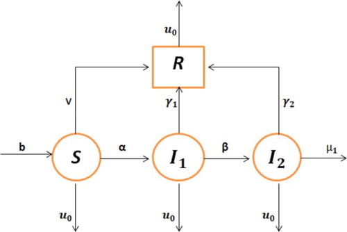
In this section, we develop a mathematical model for HBV transmission by extending the work presented in [8]. We divide the host population denoted by $T\left(t\right)$ into four compartments: susceptible individuals $S\left(t\right)$, who are not infective but have the chance to catch the disease; infected $I_1\left(t\right)$ represents those individuals who are infective with acute hepatitis; $I_2\left(t\right)$ are those individuals, who are infected with chronic hepatitis and $R\left(t\right)$ represents those individuals who have recovered after the infection with a life-time immunity. The flowchart for the transmission of HBV is given in Figure 1.

Figure 1. The flowchart representing the HBV transmission.

Thus, the mathematical model is represented by the following four differentials equations: (1) $\begin{array}{rl}\frac{\mathrm{d}S\left(t\right)}{\mathrm{d}t}& =b-\alpha S\left(t\right)I_2\left(t\right)-({\mu }_0+v)S\left(t\right),\\ \frac{\mathrm{d}{I}_1\left(t\right)}{\mathrm{d}t}& =\alpha S\left(t\right)I_2\left(t\right)-({\mu }_0+\beta +{\gamma }_1)I_1\left(t\right),\\ \frac{\mathrm{d}{I}_2\left(t\right)}{\mathrm{d}t}& =\beta I_1\left(t\right)-({\mu }_0+{\mu }_1+{\gamma }_2)I_2\left(t\right),\\ \frac{\mathrm{d}R\left(t\right)}{\mathrm{d}t}& ={\gamma }_1{I}_1\left(t\right)+{\gamma }_2{I}_2\left(t\right)+vS\left(t\right)-{\mu }_{0}R\left(t\right),\end{array}$(1) with initial conditions $S\left(0\right)\ge 0,I_1\left(0\right)\ge 0,I_2\left(0\right)\ge 0,R\left(0\right)\ge 0.$ Here b represents the birth rate, α is the moving rate from susceptible to infected with acute hepatitis B, β is the moving rate from acute stage to infected with chronic hepatitis, ${\gamma }_1$ is the recovery rate from acute stage to recovered, ${\gamma }_2$ is the recovery rate from chronic stage to recovered compartment, ${\mu }_0$ is the death rate occurring naturally, which is also called natural mortality rate, ${\mu }_1$ is the death rate occurring due to hepatitis B and v represents hepatitis B vaccination rate.

Basic reproduction number $R_0$ is defined to be the expected number of secondary infections produced by an index case or the average number of secondary infection arising from a single individual introduced into the susceptible class during its entire infectious period in a totally susceptible population [6]. We obtain the basic reproduction number $R_0$ of the model (1(1) $\begin{array}{rl}\frac{\mathrm{d}S\left(t\right)}{\mathrm{d}t}& =b-\alpha S\left(t\right)I_2\left(t\right)-({\mu }_0+v)S\left(t\right),\\ \frac{\mathrm{d}{I}_1\left(t\right)}{\mathrm{d}t}& =\alpha S\left(t\right)I_2\left(t\right)-({\mu }_0+\beta +{\gamma }_1)I_1\left(t\right),\\ \frac{\mathrm{d}{I}_2\left(t\right)}{\mathrm{d}t}& =\beta I_1\left(t\right)-({\mu }_0+{\mu }_1+{\gamma }_2)I_2\left(t\right),\\ \frac{\mathrm{d}R\left(t\right)}{\mathrm{d}t}& ={\gamma }_1{I}_1\left(t\right)+{\gamma }_2{I}_2\left(t\right)+vS\left(t\right)-{\mu }_{0}R\left(t\right),\end{array}$(1) ) as (2) $R_0=\frac{\alpha \beta b}{({\mu }_0+v)({\mu }_0+\beta +{\gamma }_1)({\mu }_0+{\mu }_1+{\gamma }_2)}.$(2)

3. Steady-state analysis

In this section, we use stability analysis theory to find steady state of our proposed model. First, we prove that the model (1(1) $\begin{array}{rl}\frac{\mathrm{d}S\left(t\right)}{\mathrm{d}t}& =b-\alpha S\left(t\right)I_2\left(t\right)-({\mu }_0+v)S\left(t\right),\\ \frac{\mathrm{d}{I}_1\left(t\right)}{\mathrm{d}t}& =\alpha S\left(t\right)I_2\left(t\right)-({\mu }_0+\beta +{\gamma }_1)I_1\left(t\right),\\ \frac{\mathrm{d}{I}_2\left(t\right)}{\mathrm{d}t}& =\beta I_1\left(t\right)-({\mu }_0+{\mu }_1+{\gamma }_2)I_2\left(t\right),\\ \frac{\mathrm{d}R\left(t\right)}{\mathrm{d}t}& ={\gamma }_1{I}_1\left(t\right)+{\gamma }_2{I}_2\left(t\right)+vS\left(t\right)-{\mu }_{0}R\left(t\right),\end{array}$(1) ) is locally asymptotically as well as globally asymptotically stable at disease-free and endemic equilibrium points. For disease-free equilibrium the model (1(1) $\begin{array}{rl}\frac{\mathrm{d}S\left(t\right)}{\mathrm{d}t}& =b-\alpha S\left(t\right)I_2\left(t\right)-({\mu }_0+v)S\left(t\right),\\ \frac{\mathrm{d}{I}_1\left(t\right)}{\mathrm{d}t}& =\alpha S\left(t\right)I_2\left(t\right)-({\mu }_0+\beta +{\gamma }_1)I_1\left(t\right),\\ \frac{\mathrm{d}{I}_2\left(t\right)}{\mathrm{d}t}& =\beta I_1\left(t\right)-({\mu }_0+{\mu }_1+{\gamma }_2)I_2\left(t\right),\\ \frac{\mathrm{d}R\left(t\right)}{\mathrm{d}t}& ={\gamma }_1{I}_1\left(t\right)+{\gamma }_2{I}_2\left(t\right)+vS\left(t\right)-{\mu }_{0}R\left(t\right),\end{array}$(1) ) is both locally and globally stable, if the value of basic reproduction number is less than unity while for the endemic equilibrium the model (1(1) $\begin{array}{rl}\frac{\mathrm{d}S\left(t\right)}{\mathrm{d}t}& =b-\alpha S\left(t\right)I_2\left(t\right)-({\mu }_0+v)S\left(t\right),\\ \frac{\mathrm{d}{I}_1\left(t\right)}{\mathrm{d}t}& =\alpha S\left(t\right)I_2\left(t\right)-({\mu }_0+\beta +{\gamma }_1)I_1\left(t\right),\\ \frac{\mathrm{d}{I}_2\left(t\right)}{\mathrm{d}t}& =\beta I_1\left(t\right)-({\mu }_0+{\mu }_1+{\gamma }_2)I_2\left(t\right),\\ \frac{\mathrm{d}R\left(t\right)}{\mathrm{d}t}& ={\gamma }_1{I}_1\left(t\right)+{\gamma }_2{I}_2\left(t\right)+vS\left(t\right)-{\mu }_{0}R\left(t\right),\end{array}$(1) ) is stable if the value of the basic reproduction number $R_0$ is greater than unity. Model (1(1) $\begin{array}{rl}\frac{\mathrm{d}S\left(t\right)}{\mathrm{d}t}& =b-\alpha S\left(t\right)I_2\left(t\right)-({\mu }_0+v)S\left(t\right),\\ \frac{\mathrm{d}{I}_1\left(t\right)}{\mathrm{d}t}& =\alpha S\left(t\right)I_2\left(t\right)-({\mu }_0+\beta +{\gamma }_1)I_1\left(t\right),\\ \frac{\mathrm{d}{I}_2\left(t\right)}{\mathrm{d}t}& =\beta I_1\left(t\right)-({\mu }_0+{\mu }_1+{\gamma }_2)I_2\left(t\right),\\ \frac{\mathrm{d}R\left(t\right)}{\mathrm{d}t}& ={\gamma }_1{I}_1\left(t\right)+{\gamma }_2{I}_2\left(t\right)+vS\left(t\right)-{\mu }_{0}R\left(t\right),\end{array}$(1) ) has a disease-free equilibrium, denoted by $E_0$ and defined as, $E_0=(S_0,0,0,R^0)$, where $S_0=b/({\mu }_0+v)$ and $R^0=vb/{\mu }_0({\mu }_0+v)$. The endemic equilibrium is given by $E^{\ast }=(S^{\ast },I_1^{\ast },I_2^{\ast },R^{\ast })$, where (3) $\begin{array}{rl}{S}^{\ast }& =\frac{1}{\alpha \beta }({\mu }_0+{\mu }_1+{\gamma }_2)({\mu }_0+\beta +{\gamma }_1),\\ I_1^{\ast }& =\frac{1}{\alpha \beta }({\mu }_0+v)({\mu }_0+{\mu }_1+{\gamma }_2)[R_0-1],\\ I_2^{\ast }& =\frac{1}{\alpha }({\mu }_0+v)[R_0-1],\\ R^{\ast }& =\frac{1}{{\mu }_0}\left[\left(\frac{{\gamma }_1}{\alpha \beta }({\mu }_0+v)({\mu }_0+{\mu }_1+{\gamma }_2)+\frac{{\gamma }_2}{\alpha }({\mu }_0+v)(R_0-1)\right)\right.\\ & +\left.\frac{v}{\alpha \beta }({\mu }_0+{\mu }_1+{\gamma }_2)({\mu }_0+\beta +{\gamma }_1)\right].\end{array}$(3) Regarding the stability of the model (1(1) $\begin{array}{rl}\frac{\mathrm{d}S\left(t\right)}{\mathrm{d}t}& =b-\alpha S\left(t\right)I_2\left(t\right)-({\mu }_0+v)S\left(t\right),\\ \frac{\mathrm{d}{I}_1\left(t\right)}{\mathrm{d}t}& =\alpha S\left(t\right)I_2\left(t\right)-({\mu }_0+\beta +{\gamma }_1)I_1\left(t\right),\\ \frac{\mathrm{d}{I}_2\left(t\right)}{\mathrm{d}t}& =\beta I_1\left(t\right)-({\mu }_0+{\mu }_1+{\gamma }_2)I_2\left(t\right),\\ \frac{\mathrm{d}R\left(t\right)}{\mathrm{d}t}& ={\gamma }_1{I}_1\left(t\right)+{\gamma }_2{I}_2\left(t\right)+vS\left(t\right)-{\mu }_{0}R\left(t\right),\end{array}$(1) ) at $E_0$ and $E^{\ast }$, we have the following results.

Theorem 3.1.

If $R_0<1,$ then the model (1(1) $\begin{array}{rl}\frac{\mathrm{d}S\left(t\right)}{\mathrm{d}t}& =b-\alpha S\left(t\right)I_2\left(t\right)-({\mu }_0+v)S\left(t\right),\\ \frac{\mathrm{d}{I}_1\left(t\right)}{\mathrm{d}t}& =\alpha S\left(t\right)I_2\left(t\right)-({\mu }_0+\beta +{\gamma }_1)I_1\left(t\right),\\ \frac{\mathrm{d}{I}_2\left(t\right)}{\mathrm{d}t}& =\beta I_1\left(t\right)-({\mu }_0+{\mu }_1+{\gamma }_2)I_2\left(t\right),\\ \frac{\mathrm{d}R\left(t\right)}{\mathrm{d}t}& ={\gamma }_1{I}_1\left(t\right)+{\gamma }_2{I}_2\left(t\right)+vS\left(t\right)-{\mu }_{0}R\left(t\right),\end{array}$(1) ) is locally asymptotically stable at disease-free equilibrium, $E_0=(b/({\mu }_0+v),0,0,vb/{\mu }_0({\mu }_0+v))$ while $E_0$ is unstable saddle point if $R_0>1$.

Proof.

To prove the result, we evaluate the Jacobian matrix for the system (1(1) $\begin{array}{rl}\frac{\mathrm{d}S\left(t\right)}{\mathrm{d}t}& =b-\alpha S\left(t\right)I_2\left(t\right)-({\mu }_0+v)S\left(t\right),\\ \frac{\mathrm{d}{I}_1\left(t\right)}{\mathrm{d}t}& =\alpha S\left(t\right)I_2\left(t\right)-({\mu }_0+\beta +{\gamma }_1)I_1\left(t\right),\\ \frac{\mathrm{d}{I}_2\left(t\right)}{\mathrm{d}t}& =\beta I_1\left(t\right)-({\mu }_0+{\mu }_1+{\gamma }_2)I_2\left(t\right),\\ \frac{\mathrm{d}R\left(t\right)}{\mathrm{d}t}& ={\gamma }_1{I}_1\left(t\right)+{\gamma }_2{I}_2\left(t\right)+vS\left(t\right)-{\mu }_{0}R\left(t\right),\end{array}$(1) ) and it is given by (4) $J=\left(\begin{array}{cccc}\alpha I_2-({\mu }_0+v)& 0& -\alpha S& 0\\ \alpha I_2& -({\mu }_0+\beta )-{\gamma }_1& \alpha S-({\mu }_0+{\mu }_1)& 0\\ 0& \beta & -{\gamma }_2& 0\\ v& {\gamma }_1& {\gamma }_2& -{\mu }_0\end{array}\right).$(4) Using $E_0=(b/({\mu }_0+v),0,0,vb/{\mu }_0({\mu }_0+v))$ in Equation (4(4) $J=\left(\begin{array}{cccc}\alpha I_2-({\mu }_0+v)& 0& -\alpha S& 0\\ \alpha I_2& -({\mu }_0+\beta )-{\gamma }_1& \alpha S-({\mu }_0+{\mu }_1)& 0\\ 0& \beta & -{\gamma }_2& 0\\ v& {\gamma }_1& {\gamma }_2& -{\mu }_0\end{array}\right).$(4) ), we obtain (5) $J\left(E_0\right)=\left(\begin{array}{cccc}-({\mu }_0+v)& 0& \frac{-\alpha b}{{\mu }_0+v}& 0\\ 0& -({\mu }_0+\beta )-{\gamma }_1& \frac{\alpha b}{{\mu }_0+v}& 0\\ 0& \beta & -({\mu }_0+{\mu }_1)-{\gamma }_2& 0\\ v& {\gamma }_1& {\gamma }_2& -{\mu }_0\end{array}\right).$(5) Two eigenvalues ${\lambda }_1$ and ${\lambda }_2$ of $J\left(E_0\right)$ are negative, ${\lambda }_1=-({\mu }_0+v)<0$, ${\lambda }_2=-{\mu }_0<0$. For the rest eigenvalues, we take the following $2\times 2$ matrix, such that (6) $A=\left(\begin{array}{cc}-({\mu }_0+\beta )-{\gamma }_1& \frac{\alpha b}{{\mu }_0+v}\\ \beta & -({\mu }_0+{\mu }_1)-{\gamma }_2\end{array}\right).$(6) Now for the Routh–Hurwitz criteria, it is sufficient to prove that, trace of A is negative and determinant of A is positive, if $R_0<1$, thus we have $\begin{array}{rl}\mathrm{Trac}\left(A\right)& =[-({\mu }_0+\beta )-{\gamma }_1+-({\mu }_0+{\mu }_1)-{\gamma }_2],\\ \mathrm{Trac}\left(A\right)& =-\left[\right({\mu }_0+\beta )+{\gamma }_1+({\mu }_0+{\mu }_1)+{\gamma }_2],\\ \mathrm{Trac}\left(A\right)& =-\left[\right(2{\mu }_0+\beta +{\mu }_1+{\gamma }_1+{\gamma }_2\left)\right].\end{array}$ Thus, $\mathrm{Trac}\left(A\right)=-\left[\right(2{\mu }_0+\beta +{\mu }_1+{\gamma }_1+{\gamma }_2\left)\right]<0$. Now for the determinant of A, we have $\begin{array}{rl}\det \left(A\right)& =\left[\left(\right({\mu }_0+\beta )+{\gamma }_1)\left(\right({\mu }_0+{\mu }_1)+{\gamma }_2)-\frac{\alpha \beta b}{{\mu }_0+v}\right],\\ \det \left(A\right)& =\left(\right({\mu }_0+\beta )+{\gamma }_1)\left(\right({\mu }_0+{\mu }_1)+{\gamma }_2)\\ & \left[1-\frac{\alpha \beta b}{({\mu }_0+v)({\mu }_0+\beta +{\gamma }_1)({\mu }_0+{\mu }_1+{\gamma }_2)}\right],\\ \det \left(A\right)& =\left(\right({\mu }_0+\beta )+{\gamma }_1)\left(\right({\mu }_0+{\mu }_1)+{\gamma }_2)[1-R_0],\end{array}$ which implies that $\det \left(A\right)$ is positive, if $R_0<1$. Therefore, $\mathrm{Trac}\left(A\right)<0$ and $\det \left(A\right)>0$ if and only if $R_0<1$. But on the other hand, if $R_0>1,$ then $\mathrm{Trac}\left(A\right)<0$ and $\det \left(A\right)<0$, which shows that the characteristic equation of A has positive and negative root, therefore $E_0$ is a unstable saddle point.

Theorem 3.2.

The model (1(1) $\begin{array}{rl}\frac{\mathrm{d}S\left(t\right)}{\mathrm{d}t}& =b-\alpha S\left(t\right)I_2\left(t\right)-({\mu }_0+v)S\left(t\right),\\ \frac{\mathrm{d}{I}_1\left(t\right)}{\mathrm{d}t}& =\alpha S\left(t\right)I_2\left(t\right)-({\mu }_0+\beta +{\gamma }_1)I_1\left(t\right),\\ \frac{\mathrm{d}{I}_2\left(t\right)}{\mathrm{d}t}& =\beta I_1\left(t\right)-({\mu }_0+{\mu }_1+{\gamma }_2)I_2\left(t\right),\\ \frac{\mathrm{d}R\left(t\right)}{\mathrm{d}t}& ={\gamma }_1{I}_1\left(t\right)+{\gamma }_2{I}_2\left(t\right)+vS\left(t\right)-{\mu }_{0}R\left(t\right),\end{array}$(1) ) is locally asymptotically stable at endemic equilibrium $E^{\ast }=(S^{\ast },I_1^{\ast },I_2^{\ast },R^{\ast }),$ if $R_0>1$ and satisfies the following conditions: $\begin{array}{rl}& \alpha \beta b<\phi ,\\ & {\phi }_1<{\phi }_2,\end{array}$ where $\begin{array}{rl}\phi & =({\mu }_0+\beta +{\gamma }_1)({\mu }_0+{\mu }_1+{\gamma }_2)[3{\mu }_0+v+\beta +{\gamma }_1+{\gamma }_2],\\ {\phi }_1& =({\mu }_0+v)({\mu }_0+\beta +{\gamma }_1){\gamma }_2,\\ {\phi }_2& =2({\mu }_0+v)({\mu }_0+{\mu }_1+{\gamma }_2)({\mu }_0+\beta +{\gamma }_1),\end{array}$ otherwise unstable.

Proof.

Using $E^{\ast }=(S^{\ast },I_1^{\ast },I_2^{\ast },R^{\ast })$ in the Jacobian matrix given in Equation (4(4) $J=\left(\begin{array}{cccc}\alpha I_2-({\mu }_0+v)& 0& -\alpha S& 0\\ \alpha I_2& -({\mu }_0+\beta )-{\gamma }_1& \alpha S-({\mu }_0+{\mu }_1)& 0\\ 0& \beta & -{\gamma }_2& 0\\ v& {\gamma }_1& {\gamma }_2& -{\mu }_0\end{array}\right).$(4) ), we obtain $J\left(E^{\ast }\right)=\left(\begin{array}{cccc}\frac{\alpha \beta b}{({\mu }_0+{\mu }_1+{\gamma }_2)({\mu }_0+\beta +{\gamma }_1)}& 0& \frac{-({\mu }_0+{\mu }_1+{\gamma }_2)({\mu }_0+\beta +{\gamma }_1)}{\beta }& 0\\ \frac{\alpha \beta b}{({\mu }_0+{\mu }_1+{\gamma }_2)({\mu }_0+\beta +{\gamma }_1)}-({\mu }_0+v)& -({\mu }_0+\beta )-{\gamma }_1& \frac{({\mu }_0+{\mu }_1+{\gamma }_2)({\mu }_0+\beta +{\gamma }_1)}{\beta }& 0\\ 0& \beta & -{\gamma }_2& 0\\ v& {\gamma }_1& {\gamma }_2& -{\mu }_0\end{array}\right).$

Clearly, one eigenvalue of $J\left(E^{\ast }\right)$ is negative that is ${\lambda }_1=-{\mu }_0<0$. For the remaining eigenvalues, we construct the $3\times 3$ matrix and it is given by (7) $B=\left(\begin{array}{ccc}\frac{\alpha \beta b}{({\mu }_0+{\mu }_1+{\gamma }_2)({\mu }_0+\beta +{\gamma }_1)}& 0& \frac{-({\mu }_0+{\mu }_1+{\gamma }_2)({\mu }_0+\beta +{\gamma }_1)}{\beta }\\ \frac{\alpha \beta b}{({\mu }_0+{\mu }_1+{\gamma }_2)({\mu }_0+\beta +{\gamma }_1)}-({\mu }_0+v)& -({\mu }_0+\beta )-{\gamma }_1& \frac{({\mu }_0+{\mu }_1+{\gamma }_2)({\mu }_0+\beta +{\gamma }_1)}{\beta }\\ 0& \beta & -{\gamma }_2\end{array}\right).$(7) The characteristic polynomial of the above matrix becomes (8) $\psi \left(\lambda \right)={\lambda }^3+a_1{\lambda }^2+a_2\lambda +a_3,$(8) where $\begin{array}{rl}{a}_1& =({\mu }_0+v)+({\mu }_0+\beta +{\gamma }_1)+{\gamma }_2-({\mu }_0+v)(R_0-1),\\ a_2& =({\mu }_0+v)({\mu }_0+\beta +{\gamma }_1)+({\mu }_0+v){\gamma }_2-({\mu }_0+{\mu }_1+{\gamma }_2)({\mu }_0+\beta +{\gamma }_1)\\ & +({\mu }_0+\beta +{\gamma }_1){\gamma }_2-\left[\right({\mu }_0+v)+({\mu }_0+v\left){\gamma }_2\right](R_0-1),\\ a_3& =({\mu }_0+v)({\mu }_0+\beta +{\gamma }_1){\gamma }_2-({\mu }_0+v)({\mu }_0+{\mu }_1+{\gamma }_2)({\mu }_0+\beta +{\gamma }_1)\\ & +\left[2\right({\mu }_0+v\left)\right({\mu }_0+{\mu }_1+{\gamma }_2\left)\right({\mu }_0+\beta +{\gamma }_1)-({\mu }_0+v\left)\right({\mu }_0+\beta +{\gamma }_1\left){\gamma }_2\right](R_0-1).\end{array}$ Here for the Routh–Hurwitz criteria, we need to prove that, $a_i>0$, for i=1,2,3 and $a_1{a}_2>a_3$. Thus, $a_1>0$, $a_3>0$ and $a_1{a}_2>a_3$ are possible only if $R_0>1$, $\alpha \beta b<\phi$ and ${\phi }_1<{\phi }_2.$ Therefore, by Routh–Hurwitz criteria all the roots of the characteristic polynomial $\psi \left(\lambda \right)$ have negative real parts. Hence $E^{\ast }$ is locally asymptotically stable, which completes the proof.

Theorem 3.3.

If $R_0\le 1,$ then the model (1(1) $\begin{array}{rl}\frac{\mathrm{d}S\left(t\right)}{\mathrm{d}t}& =b-\alpha S\left(t\right)I_2\left(t\right)-({\mu }_0+v)S\left(t\right),\\ \frac{\mathrm{d}{I}_1\left(t\right)}{\mathrm{d}t}& =\alpha S\left(t\right)I_2\left(t\right)-({\mu }_0+\beta +{\gamma }_1)I_1\left(t\right),\\ \frac{\mathrm{d}{I}_2\left(t\right)}{\mathrm{d}t}& =\beta I_1\left(t\right)-({\mu }_0+{\mu }_1+{\gamma }_2)I_2\left(t\right),\\ \frac{\mathrm{d}R\left(t\right)}{\mathrm{d}t}& ={\gamma }_1{I}_1\left(t\right)+{\gamma }_2{I}_2\left(t\right)+vS\left(t\right)-{\mu }_{0}R\left(t\right),\end{array}$(1) ) is globally asymptotically stable at disease-free equilibrium, $E_0=(S_0,0,0,R^0)$ and unstable otherwise.

Proof.

To show the global stability of the model (1(1) $\begin{array}{rl}\frac{\mathrm{d}S\left(t\right)}{\mathrm{d}t}& =b-\alpha S\left(t\right)I_2\left(t\right)-({\mu }_0+v)S\left(t\right),\\ \frac{\mathrm{d}{I}_1\left(t\right)}{\mathrm{d}t}& =\alpha S\left(t\right)I_2\left(t\right)-({\mu }_0+\beta +{\gamma }_1)I_1\left(t\right),\\ \frac{\mathrm{d}{I}_2\left(t\right)}{\mathrm{d}t}& =\beta I_1\left(t\right)-({\mu }_0+{\mu }_1+{\gamma }_2)I_2\left(t\right),\\ \frac{\mathrm{d}R\left(t\right)}{\mathrm{d}t}& ={\gamma }_1{I}_1\left(t\right)+{\gamma }_2{I}_2\left(t\right)+vS\left(t\right)-{\mu }_{0}R\left(t\right),\end{array}$(1) ) at $E_0$, we construct the Lyapunov function and it is given by (9) $\mathrm{\Phi }\left(t\right)=d_1(S-S_0)+d_2{I}_1+d_3{I}_2,$(9) where $d_i$ for i=1,2,3 are some positive constants to be chosen latter. Now calculating the time derivative of Equation (9(9) $\mathrm{\Phi }\left(t\right)=d_1(S-S_0)+d_2{I}_1+d_3{I}_2,$(9) ) and then using the model (1(1) $\begin{array}{rl}\frac{\mathrm{d}S\left(t\right)}{\mathrm{d}t}& =b-\alpha S\left(t\right)I_2\left(t\right)-({\mu }_0+v)S\left(t\right),\\ \frac{\mathrm{d}{I}_1\left(t\right)}{\mathrm{d}t}& =\alpha S\left(t\right)I_2\left(t\right)-({\mu }_0+\beta +{\gamma }_1)I_1\left(t\right),\\ \frac{\mathrm{d}{I}_2\left(t\right)}{\mathrm{d}t}& =\beta I_1\left(t\right)-({\mu }_0+{\mu }_1+{\gamma }_2)I_2\left(t\right),\\ \frac{\mathrm{d}R\left(t\right)}{\mathrm{d}t}& ={\gamma }_1{I}_1\left(t\right)+{\gamma }_2{I}_2\left(t\right)+vS\left(t\right)-{\mu }_{0}R\left(t\right),\end{array}$(1) ), we obtain (10) $\begin{array}{rl}\frac{\mathrm{d}\mathrm{\Phi }}{\mathrm{d}t}& =d_1[b-\alpha S{I}_2-({\mu }_0+v\left)S\right]+d_2[\alpha S{I}_2-({\mu }_0+\beta +{\gamma }_1\left)\right]I_1\\ & +d_3[\beta I_1-({\mu }_0+{\mu }_1+{\gamma }_2\left)\right]I_2.\end{array}$(10) By assuming the positive constants $d_1=d_2={\mu }_0+v$, $d_3=\alpha b/({\mu }_0+{\mu }_1+{\gamma }_2)$ and $S_0=b/({\mu }_0+v)$ in Equation (10(10) $\begin{array}{rl}\frac{\mathrm{d}\mathrm{\Phi }}{\mathrm{d}t}& =d_1[b-\alpha S{I}_2-({\mu }_0+v\left)S\right]+d_2[\alpha S{I}_2-({\mu }_0+\beta +{\gamma }_1\left)\right]I_1\\ & +d_3[\beta I_1-({\mu }_0+{\mu }_1+{\gamma }_2\left)\right]I_2.\end{array}$(10) ), we obtain $\begin{array}{rl}\frac{\mathrm{d}\mathrm{\Phi }}{\mathrm{d}t}& =({\mu }_0+v)\left[\right(S_0({\mu }_0+v)-\alpha S{I}_2-({\mu }_0+v)S\left)\right]\\ & +\left({\mu }_0+v\right)\left[\right(\alpha S{I}_2-\left({\mu }_0+\beta +{\gamma }_1\right)I_1\left]+\frac{\alpha b}{{\mu }_0+{\mu }_1+{\gamma }_2}\right[\beta I_1-\left({\mu }_0+{\mu }_1+{\gamma }_2\right)]I_2.\end{array}$ Simplifying and rewriting the above equation after little rearrangement, we obtain $\frac{\mathrm{d}\mathrm{\Phi }}{\mathrm{d}t}=-({\mu }_0+v{)}^2[S-S_0]-[({\mu }_0+v)({\mu }_0+\beta +{\gamma }_1)(1-R_0)]I_1-\alpha b{I}_2.$ Thus, $\mathrm{d}\mathrm{\Phi }/\mathrm{d}t<0$, if $R_0\le 1$. Also $\mathrm{d}\mathrm{\Phi }/\mathrm{d}t=0$ if and only if $S=S_0,$ $I_1=0$ and $I_2=0$. Therefore, LaSalle's invariant principle [9], then implies that $E_0$ is globally asymptotically stable. This completes the proof.

Theorem 3.4.

The endemic equilibrium state $E_1=(S^{\ast },I_1^{\ast },I_2^{\ast },R^{\ast })$ of the model (1(1) $\begin{array}{rl}\frac{\mathrm{d}S\left(t\right)}{\mathrm{d}t}& =b-\alpha S\left(t\right)I_2\left(t\right)-({\mu }_0+v)S\left(t\right),\\ \frac{\mathrm{d}{I}_1\left(t\right)}{\mathrm{d}t}& =\alpha S\left(t\right)I_2\left(t\right)-({\mu }_0+\beta +{\gamma }_1)I_1\left(t\right),\\ \frac{\mathrm{d}{I}_2\left(t\right)}{\mathrm{d}t}& =\beta I_1\left(t\right)-({\mu }_0+{\mu }_1+{\gamma }_2)I_2\left(t\right),\\ \frac{\mathrm{d}R\left(t\right)}{\mathrm{d}t}& ={\gamma }_1{I}_1\left(t\right)+{\gamma }_2{I}_2\left(t\right)+vS\left(t\right)-{\mu }_{0}R\left(t\right),\end{array}$(1) ) is globally asymptotically stable, if $R_0>1,$ otherwise unstable.

Proof.

To prove the global stability of the model (1(1) $\begin{array}{rl}\frac{\mathrm{d}S\left(t\right)}{\mathrm{d}t}& =b-\alpha S\left(t\right)I_2\left(t\right)-({\mu }_0+v)S\left(t\right),\\ \frac{\mathrm{d}{I}_1\left(t\right)}{\mathrm{d}t}& =\alpha S\left(t\right)I_2\left(t\right)-({\mu }_0+\beta +{\gamma }_1)I_1\left(t\right),\\ \frac{\mathrm{d}{I}_2\left(t\right)}{\mathrm{d}t}& =\beta I_1\left(t\right)-({\mu }_0+{\mu }_1+{\gamma }_2)I_2\left(t\right),\\ \frac{\mathrm{d}R\left(t\right)}{\mathrm{d}t}& ={\gamma }_1{I}_1\left(t\right)+{\gamma }_2{I}_2\left(t\right)+vS\left(t\right)-{\mu }_{0}R\left(t\right),\end{array}$(1) ) at endemic equilibrium point $E^{\ast }=(S^{\ast },I_1^{\ast },I_2^{\ast },R^{\ast })$, we define the Lyapunov function which is given by (11) $\mathrm{\Psi }\left(t\right)=\frac{1}{2}\left[\right(S-S^{\ast })+(I_1-I_1^{\ast })+(I_2-I_2^{\ast }){]}^2.$(11) Calculating the derivative of the above function with respect to time and then using the model (1(1) $\begin{array}{rl}\frac{\mathrm{d}S\left(t\right)}{\mathrm{d}t}& =b-\alpha S\left(t\right)I_2\left(t\right)-({\mu }_0+v)S\left(t\right),\\ \frac{\mathrm{d}{I}_1\left(t\right)}{\mathrm{d}t}& =\alpha S\left(t\right)I_2\left(t\right)-({\mu }_0+\beta +{\gamma }_1)I_1\left(t\right),\\ \frac{\mathrm{d}{I}_2\left(t\right)}{\mathrm{d}t}& =\beta I_1\left(t\right)-({\mu }_0+{\mu }_1+{\gamma }_2)I_2\left(t\right),\\ \frac{\mathrm{d}R\left(t\right)}{\mathrm{d}t}& ={\gamma }_1{I}_1\left(t\right)+{\gamma }_2{I}_2\left(t\right)+vS\left(t\right)-{\mu }_{0}R\left(t\right),\end{array}$(1) ), we obtain $\begin{array}{rl}\frac{\mathrm{d}\mathrm{\Psi }}{\mathrm{d}t}& =\left[\right(S-S^{\ast })+(I_1-I_1^{\ast })+(I_2-I_2^{\ast }\left)\right][b-({\mu }_0+v)S-({\mu }_0+{\gamma }_1)I_1\\ & -({\mu }_0+{\mu }_1+{\gamma }_2)I_2].\end{array}$ By using Equation (3(3) $\begin{array}{rl}{S}^{\ast }& =\frac{1}{\alpha \beta }({\mu }_0+{\mu }_1+{\gamma }_2)({\mu }_0+\beta +{\gamma }_1),\\ I_1^{\ast }& =\frac{1}{\alpha \beta }({\mu }_0+v)({\mu }_0+{\mu }_1+{\gamma }_2)[R_0-1],\\ I_2^{\ast }& =\frac{1}{\alpha }({\mu }_0+v)[R_0-1],\\ R^{\ast }& =\frac{1}{{\mu }_0}\left[\left(\frac{{\gamma }_1}{\alpha \beta }({\mu }_0+v)({\mu }_0+{\mu }_1+{\gamma }_2)+\frac{{\gamma }_2}{\alpha }({\mu }_0+v)(R_0-1)\right)\right.\\ & +\left.\frac{v}{\alpha \beta }({\mu }_0+{\mu }_1+{\gamma }_2)({\mu }_0+\beta +{\gamma }_1)\right].\end{array}$(3) ) and after some simple simplification, we obtain $\begin{array}{rl}\frac{\mathrm{d}\mathrm{\Psi }}{\mathrm{d}t}& =\left[\right(S-S^{\ast })+(I_1-I_1^{\ast })+(I_2-I_2^{\ast }\left)\right]\left[\right({\mu }_0+{\gamma }_1)I_1^{\ast }+\beta I_1^{\ast }+({\mu }_0+v)S^{\ast }-({\mu }_0+v)S\\ & -({\mu }_0+{\gamma }_1)I_1-({\mu }_0+{\mu }_1+{\gamma }_2)I_2],\\ \frac{\mathrm{d}\mathrm{\Psi }}{\mathrm{d}t}& =-\left[\right(S-S^{\ast })+(I_1-I_1^{\ast })+(I_2-I_2^{\ast }\left)\right]\left[\right({\mu }_0+{\gamma }_1\left)\right(I_1-I_1^{\ast })+(S-S^{\ast }\left)\right({\mu }_0+v\left)\right]\\ & +\frac{1}{\alpha }({\mu }_0+v)({\mu }_0+{\mu }_1+{\gamma }_2)(R_0-1)-({\mu }_0+{\mu }_1+{\gamma }_2)I_2.\end{array}$ After some rearrangement and using Equation (3(3) $\begin{array}{rl}{S}^{\ast }& =\frac{1}{\alpha \beta }({\mu }_0+{\mu }_1+{\gamma }_2)({\mu }_0+\beta +{\gamma }_1),\\ I_1^{\ast }& =\frac{1}{\alpha \beta }({\mu }_0+v)({\mu }_0+{\mu }_1+{\gamma }_2)[R_0-1],\\ I_2^{\ast }& =\frac{1}{\alpha }({\mu }_0+v)[R_0-1],\\ R^{\ast }& =\frac{1}{{\mu }_0}\left[\left(\frac{{\gamma }_1}{\alpha \beta }({\mu }_0+v)({\mu }_0+{\mu }_1+{\gamma }_2)+\frac{{\gamma }_2}{\alpha }({\mu }_0+v)(R_0-1)\right)\right.\\ & +\left.\frac{v}{\alpha \beta }({\mu }_0+{\mu }_1+{\gamma }_2)({\mu }_0+\beta +{\gamma }_1)\right].\end{array}$(3) ) in the above, we have $\begin{array}{rl}\frac{\mathrm{d}\mathrm{\Psi }}{\mathrm{d}t}& =-\left[\right(S-S^{\ast })+(I_1-I_1^{\ast })+(I_2-I_2^{\ast }\left)\right]\left[\right({\mu }_0+{\gamma }_1\left)\right(I_1-I_1^{\ast })+(S-S^{\ast }\left)\right({\mu }_0+v\left)\right]\\ & +\left[\right({\mu }_0+{\mu }_1+{\gamma }_2\left)\right]\left[\frac{1}{\alpha }({\mu }_0+v)(R_0-1)-I_2\right],\\ \frac{\mathrm{d}\mathrm{\Psi }}{\mathrm{d}t}& =-\left[\right(S-S^{\ast })+(I_1-I_1^{\ast })+(I_2-I_2^{\ast }\left)\right]\left[\right({\mu }_0+{\gamma }_1\left)\right(I_1-I_1^{\ast })+(S-S^{\ast }\left)\right({\mu }_0+v\left)\right]\\ & -\left[\right({\mu }_0+{\mu }_1+{\gamma }_2\left)\right](I_2-I_2^{\ast }).\end{array}$ Hence $\mathrm{d}\mathrm{\Psi }/\mathrm{d}t\le 0$ for all $(S^{\ast },I_1^{\ast },I_2^{\ast },R^{\ast }).$ The equality $\mathrm{d}\mathrm{\Psi }/\mathrm{d}t=0$ holds, only for $S=S^{\ast },I_1=I_1^{\ast },I_2=I_2^{\ast }.$ Then the endemic equilibrium $E^{\ast }$ is the only positively invariant set containing in $\left[\right(S,I_1,I_2,R),S=S^{\ast },I_1=I_1^{\ast },I_2=I_2^{\ast },R=R^{\ast }].$ Therefore, the positive $E^{\ast }$ is globally asymptotically stable.

4. Numerical simulation

In this section, we verify some of our analytical results by using the numerical method. Numerical simulations are easily understandable as compared with the analytical results, which are very complex. Here, the simulation of our paper should be considered from a qualitative point of view, but not on the quantitative point of view. However, some of the parameters are taken in such a way so that it would be much more biologically feasible. This shows that instead of real-world data using the numerical analysis, experimental data are considered for the simulation, which is a powerful tool having a great interest.

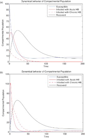
For numerical simulation we consider a set of parameters that is b=0.4, $\alpha =0.005$, $\beta =0.01$, ${\mu }_0=0.03$, ${\mu }_1=0.002$, ${\gamma }_1=0.05$, ${\gamma }_2=0.06$ and v=0.02. The numerical result in Figure 2(a) of the model (1) shows that the disease-free equilibrium is locally as well as globally asymptotically stable. Because in this case the contact rates α and β are very small, while the recovery rate is very high, so the reproduction number $R_0$ is less than one. We choose another set of parameters that are b=0.4, $\alpha =0.05$, $\beta =0.1$, ${\mu }_0=0.03$, ${\mu }_1=0.04$, ${\gamma }_1=0.05$, ${\gamma }_2=0.06$ and v=0.02. This value of parameters of the proposed model (1) has two equilibria, disease-free and endemic equilibrium. The endemic equilibrium is locally asymptotically stable (see Figure 2(b)). Furthermore, the parameter value also satisfied $R_0>1$ and the conditions of Theorem 3.2 that is $\alpha \beta b<\phi$, ${\phi }_1<{\phi }_2$ hold. This ensures the verification of analytical result of Theorem 3.2.

Figure 2. The plot shows the solution curves at the disease-free and endemic equilibrium with respect to set of parameters $A_1$ and $A_2$.

5. Optimal control application

To control the spread of HBV infection in the community, we apply optimal control techniques. Optimal control is one of the useful mathematical tools through which we are able to design the control strategy for controlling various kind of infectious diseases. To develop a control strategy, we use the optimal control theory [24,25]. Our purpose here is to reduce HBV infection from the population by maximizing the number of susceptible $S\left(t\right)$ and recovered individuals $R\left(t\right)$ and minimizing the number of infected with acute hepatitis B individuals $I_1\left(t\right)$, infected with chronic hepatitis B individuals $I_2\left(t\right)$ by using the time-dependent control variables isolation $u_1\left(t\right)$ of infected and non-infected individuals, treatment $u_2\left(t\right)$ and hepatitis B vaccination $u_3\left(t\right)$.

In the system $\left(1\right)$, we have four state variables $S\left(t\right)$, $I_1\left(t\right)$, $I_2\left(t\right)$ and $R\left(t\right)$. For the control problem, we consider the three control variables, namely isolation $u_1\left(t\right)$ of infected and non-infected individuals treatment $u_2\left(t\right)$ of infected individuals and vaccination $u_3\left(t\right)$. Thus, we have the following optimal control problem to minimize the objective functional (12) $J(u_1,u_2,u_3)={\int }_0^T\left[A_{1}S\left(t\right)+A_2{I}_1\left(t\right)+A_3{I}_2\left(t\right)+\frac{1}{2}\left(B_1{u}_1^2\right(t)+B_2{u}_2^2(t\left)\right)+B_3{u}_3\left(t\right)\right]\mathrm{d}t,$(12) subject to (13) $\begin{array}{rl}\frac{\mathrm{d}S\left(t\right)}{\mathrm{d}t}& =b-\alpha S\left(t\right)I_2\left(t\right)(1-u_1(t\left)\right)-{\mu }_{0}S\left(t\right)-u_3\left(t\right)S\left(t\right),\\ \frac{\mathrm{d}{I}_1\left(t\right)}{\mathrm{d}t}& =\alpha S\left(t\right)I_2\left(t\right)(1-u_1(t\left)\right)-({\mu }_0+\beta +{\gamma }_1)I_1\left(t\right)-\left(u_2\right(t)+u_3(t\left)\right)I_1\left(t\right),\\ \frac{\mathrm{d}{I}_2\left(t\right)}{\mathrm{d}t}& =\beta I_1\left(t\right)-({\mu }_0+{\mu }_1+{\gamma }_2)I_2\left(t\right)-\left(u_2\right(t)+u_3(t\left)\right)I_2\left(t\right),\\ \frac{\mathrm{d}R\left(t\right)}{\mathrm{d}t}& ={\gamma }_1{I}_1\left(t\right)+{\gamma }_2{I}_2\left(t\right)+u_3\left(t\right)S\left(t\right)-{\mu }_{0}R\left(t\right)+\left(u_2\right(t)+u_3(t\left)\right)\left(I_1\right(t)+I_2(t\left)\right),\end{array}$(13) with initial conditions $S\left(0\right)\ge 0,I_1\left(0\right)\ge 0,I_2\left(0\right)\ge 0,R\left(0\right)\ge 0.$ In Equation (12) $A_1$, $A_2$ and $A_3$ represent the weight constants of susceptible individuals $S\left(t\right)$, infected with acute-infected hepatitis B individuals $I_1\left(t\right)$ and infected with chronic individuals $I_2\left(t\right)$, respectively. Furthermore, in the objective functional $B_1$, $B_2$ and $B_3$ are the weight constants for the isolation of infected and non-infected, treatment and vaccination controls. The terms $\frac{1}{2}{B}_1{u}_1^2$, $\frac{1}{2}{B}_2{u}_2^2$ and $\frac{1}{2}{B}_3{u}_3^2$ describe the cost associated with isolation, treatment and vaccination. Our goal is to find the control function, such that (14) $J(u_1^{\ast },u_2^{\ast },u_3^{\ast })=\min \left\{J\right(u_1,u_2,u_3),u_1,u_2,u_3\in U\}$(14) subject to the system (13), where the control set is defined as (15) $U=\left\{\right(u_1,u_2,u_3\left)/u_i\right(t\left)\text{is Lebesgue measurable on}\right[0,1],0\le u_i(t)\le 1,i=1,2,3\}.$(15)

6. Existence of optimal control problem

To show the existence of the control problem, we consider the control system (13) with initial condition at time t=0. For bounded Lebesgue measurable controls, positive initial conditions and positive bounded solutions to the state system exist [2]. In order to find the optimal solution, let us go back to the optimal control problem (13) and (14). So first we need to define the Lagrangian and Hamiltonian for the optimal control problems (13) and (14). In fact the Lagrangian for the optimal control problem is given by the following equation: (16) $L(S,I_1,I_2,u_1,u_2,u_3)=A_{1}S\left(t\right)+A_2{I}_1\left(t\right)+A_3{I}_2\left(t\right)+\left[\frac{1}{2}\right(B_1{u}_1^2+B_2{u}_2^2+B_3{u}_3^2\left)\right].$(16) To seek the minimal value of the Lagrangian, we define Hamiltonian H for the optimal control problem as (17) $H=L(S,I_1,I_2,u_1,u_2,u_3)+{\lambda }_1\frac{\mathrm{d}S\left(t\right)}{\mathrm{d}t}+{\lambda }_2\frac{\mathrm{d}{I}_1}{\mathrm{d}t}+{\lambda }_3\frac{\mathrm{d}{I}_2}{\mathrm{d}t}+{\lambda }_4\frac{\mathrm{d}R\left(t\right)}{\mathrm{d}t}.$(17) Thus for the existence of our control problem, we have the following results.

Theorem 6.1.

There exists an optimal control $u^{\ast }=(u_1^{\ast },u_2^{\ast })\in U,$ such that $J(u_1^{\ast },u_2^{\ast },u_3^{\ast })=\min J(u_1,u_2,u_3)$ subject to the control system (13) with initial condition.

Proof.

To prove the existence of an optimal control we use techniques presented in [7,24]. Since both the control variables and the state variables are non-negative values. So in this minimizing problem, the necessary convexity of the objective functional define in Equation (12) in $u_1\left(t\right)$, $u_2\left(t\right)$ and $u_3\left(t\right)$ is satisfied. The control variables set $u_1,u_2,u_3\in U$ is also convex and closed by definition. The optimal system is bounded, which ensure the compactness needed for the existence of the optimal control. Further the integrand in the objective functional $A_{1}S\left(t\right)+A_2{I}_1\left(t\right)+A_3{I}_2\left(t\right)+\frac{1}{2}(B_1{u}_1^2+B_2{u}_2^2,B_3{u}_2^3)$ is convex on the control set U, which completes the proof.

Next, we find the optimal solution of our proposed control problem. In order to do this, we use the Pontryagin maximum principle [25]. By using this principle the Hamiltonian is given by (18) $H(t,x(t),u(t),\lambda (t\left)\right)=f(t,x(t),u(t)+\lambda (t\left)g\right(x\left(\right(t),u(t\left)\right).$(18) If $(x^{\ast },u^{\ast })$ is an optimal solution of our proposed optimal control problem, then there exists a non-trivial vector function $\lambda \left(t\right)=\left({\lambda }_1\right(t),{\lambda }_2(t),\dots ,{\lambda }_n(t\left)\right)$, such that (19) $\begin{array}{r}\frac{\mathrm{d}x}{\mathrm{d}t}=\frac{\mathrm{\partial }H(t,x(t),u(t),\lambda (t\left)\right)}{\mathrm{\partial }\lambda },\\ 0=\frac{\mathrm{\partial }H(t,x(t),u(t),\lambda (t\left)\right)}{\mathrm{\partial }u},\\ \lambda (t{)}^{\mathrm{\prime }}=-\frac{\mathrm{\partial }H(t,x(t),u(t),\lambda (t\left)\right)}{\mathrm{\partial }x}.\end{array}$(19) Now, we apply the necessary condition to the Hamiltonian, so we have the following results.

Theorem 6.2.

Let $S^{\ast },$ $I_1^{\ast },$ $I_2^{\ast }$ and $R^{\ast }$ be optimal state solution with associated optimal control variables $(u_1^{\ast },u_2^{\ast },u_3^{\ast })$ for the optimal control problems (12) and (13). Then there exist adjoint variables ${\lambda }_1\left(t\right),$ ${\lambda }_2\left(t\right),$ ${\lambda }_3\left(t\right)$ and ${\lambda }_4\left(t\right),$ satisfying (20) $\begin{array}{rl}{\lambda }_1^{\mathrm{\prime }}\left(t\right)& =-A_1+\left({\lambda }_1\right(t)-{\lambda }_2(t\left)\right)\alpha I_2^{\ast }(1-u_1^{\ast }(t\left)\right)+\left({\lambda }_1\right(t)-{\lambda }_4(t\left)\right)u_3^{\ast }+{\lambda }_1\left(t\right){\mu }_0,\\ {\lambda }_2^{\mathrm{\prime }}\left(t\right)& =-A_2+\left({\lambda }_2\right(t)-{\lambda }_4(t\left)\right)(u_2^{\ast }+u_3^{\ast })+\left({\lambda }_2\right(t)-{\lambda }_3(t\left)\right)\beta +\left({\lambda }_2\right(t)-{\lambda }_4(t\left)\right){\gamma }_1\\ & +{\lambda }_2\left(t\right){\mu }_0,\\ {\lambda }_3^{\mathrm{\prime }}\left(t\right)& =-A_3+\left({\lambda }_1\right(t)-{\lambda }_2(t\left)\right)\alpha S^{\ast }(1-u_1^{\ast })+\left({\lambda }_3\right(t)-{\lambda }_4(t\left)\right)(u_2^{\ast }+u_3^{\ast })\\ & +\left({\lambda }_3\right(t)-{\lambda }_4(t\left)\right){\gamma }_2+{\lambda }_3\left(t\right)({\mu }_0+{\mu }_1),\\ {\lambda }_4^{\mathrm{\prime }}\left(t\right)& ={\lambda }_4\left(t\right){\mu }_0,\end{array}$(20) with transversality conditions (boundary conditions) (21) ${\lambda }_i\left(T\right)=0\mathrm{for}i=1,2,3,4.$(21) Furthermore, the optimal controls variables $u_1^{\ast }\left(t\right)$, $u_2^{\ast }\left(t\right)$ and $u_3^{\ast }\left(t\right)$ are given by (22) $\begin{array}{rl}{u}_1^{\ast }\left(t\right)& =\max \left\{\min \left\{\frac{\alpha S^{\ast }{I}_2^{\ast }}{B_1}\left({\lambda }_2\right(t)-{\lambda }_1(t\left)\right),1\right\},0\right\},\end{array}$(22) (23) $\begin{array}{rl}{u}_2^{\ast }\left(t\right)& =\max \left\{\min \left\{\frac{1}{B_2}\left(\right({\lambda }_2\left(t\right)-{\lambda }_4\left(t\right))I_1^{\ast }+({\lambda }_3\left(t\right)-{\lambda }_4\left(t\right)\left)I_2^{\ast }\right),1\right\},0\right\},\end{array}$(23) (24) $\begin{array}{rl}{u}_3^{\ast }\left(t\right)& =\max \left\{\min \left\{\frac{1}{B_3}\left({\lambda }_1\right(t)S^{\ast }+({\lambda }_2\left(t\right)-{\lambda }_4\left(t\right))I_1^{\ast }+({\lambda }_3\left(t\right)-{\lambda }_4\left(t\right)\left)I_2^{\ast }\right),1\right\},0\right\}.\end{array}$(24)

Proof.

To determine the adjoint equation (20) and the transversality condition (21), we use the Hamiltonian (17). By setting $S\left(t\right)=S^{\ast }$, $I_1\left(t\right)=I_1^{\ast }$, $I_2\left(t\right)=I_2^{\ast }$ and $R\left(t\right)=R^{\ast }$ and differentiating the Hamiltonian with respect to $S\left(t\right)$, $I_1\left(t\right)$, $I_2\left(t\right)$ and $R\left(t\right)$, respectively, we will get the required adjoint system (20). Furthermore, to obtain $u_1^{\ast }$, $u_2^{\ast }$ and $u_3^{\ast }$, we differentiating Hamiltonian with respect to $u_1$, $u_2$ and $u_3$, respectively, and then solving $\mathrm{\partial }H/\mathrm{\partial }{u}_1=0$, $\mathrm{\partial }H/\mathrm{\partial }{u}_2=0$ and $\mathrm{\partial }H/\mathrm{\partial }{u}_3=0$ on the interior of the control set and using the optimality condition. Finally by using the property of control space U, we obtain Equation (22), which completes the proof.

Here, we call the formulas (22) for $u^{\ast }=(u_1^{\ast },u_2^{\ast },u_3^{\ast })$ with the characterization of optimal controls. The state variables and the optimal controls variables are found by solving the optimality system, which contain the state system (13), the adjoint system (20), initial conditions and boundary conditions, together with the characterization of the optimal controls $(u_1^{\ast },u_2^{\ast },u_3^{\ast }).$ In addition, the second derivatives of the Lagrangian with respect to $u_1$, $u_2$ and $u_3$ are positive, which make sure that the optimal problem is minimum at control $u_1^{\ast }$, $u_2^{\ast }$ and $u_3^{\ast }$. By putting the values of $u_1^{\ast }$, $u_2^{\ast }$ and $u_3^{\ast }$ in the control system (13), we obtain the following system: (25) $\begin{array}{rl}\frac{\mathrm{d}{S}^{\ast }\left(t\right)}{\mathrm{d}t}& =b-\alpha S^{\ast }\left(t\right)I_2^{\ast }\left(t\right)(1-u_1^{\ast })-{\mu }_0{S}^{\ast }-u_3^{\ast }{S}^{\ast },\\ \frac{\mathrm{d}{I}_1^{\ast }\left(t\right)}{\mathrm{d}t}& =\alpha S^{\ast }{I}_2^{\ast }(1-u_1^{\ast })-({\mu }_0+\beta +{\gamma }_1)I_1^{\ast }-(u_2^{\ast }+u_3^{\ast })I_1^{\ast },\\ \frac{\mathrm{d}{I}_2^{\ast }\left(t\right)}{\mathrm{d}t}& =\beta I_1^{\ast }-({\mu }_0+{\mu }_1+{\gamma }_2)I_2^{\ast }-(u_2^{\ast }+u^{\ast })I_2^{\ast },\\ \frac{\mathrm{d}{R}^{\ast }\left(t\right)}{\mathrm{d}t}& ={\gamma }_1{I}_1^{\ast }+{\gamma }_2{I}_2^{\ast }+u_3^{\ast }{S}^{\ast }+v{S}^{\ast }\left(t\right)+(u_2^{\ast }+u_3^{\ast })(I_1^{\ast }+I_2^{\ast })-{\mu }_0{R}^{\ast }.\end{array}$(25) In the next section, we solve the optimality system, i.e. Equations (20)–(13) numerically.

7. Numerical results of the control problem

In this section, we solve the optimality system (20)–(23) by using the Runge–Kutta method of order four. To do this, first we solve the state system (23) by the Runge–Kutta fourth-order scheme with initial condition forward in time $[0,20]$ and then solving the adjoint system (20) by the backward Runge–Kutta fourth-order scheme in the same interval of time with the help of transversality condition and the solution of state system (23). For the simulation purposes, we use the parameters' value as follows: $\alpha =0.8$, $\beta =0.025$, b=0.0121, ${\gamma }_1=0.05$, ${\gamma }_2=0.5$, ${\mu }_0=0.0121$ and ${\mu }_1=\mathrm{0.02.}$ In which the parameters $\alpha =0.8$, b=0.0121, ${\mu }_0=0.0121$ are taken from [7,18,26] and the remaining are assumed as biologically feasible values. Furthermore, the weight constants are assumed to be $A_1=400$, $A_2=1000$, $A_3=1000$, $B_1=0.001$, $B_2=0.34$ and $B_3=\mathrm{0.45.}$ So we obtain the following results presented from Figures 3 to 9.

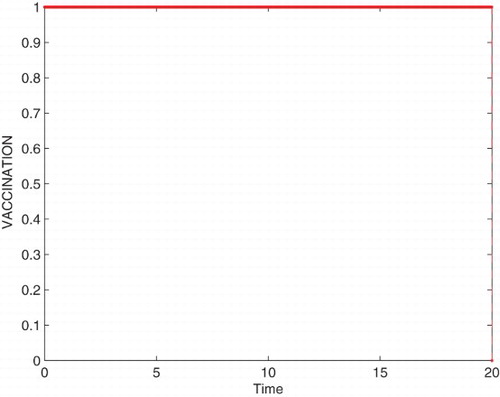
Figures 3–6 represent the dynamic of susceptible, acute-infected individuals with hepatitis B, chronically infected individuals with hepatitis B and recovered individuals, respectively. Figures 7–9 represent the dynamic of control variables isolation, treatment and vaccination, respectively. Our main objective of applying the optimal control tool is to minimize the number of infected individuals and maximize the number of non-infected individuals, which are clearly shown by the numerical results.

Figure 3. Population of susceptible with and without control.

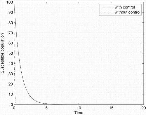
Figure 4. Population of hepatitis B acute-infected individuals with and without control.

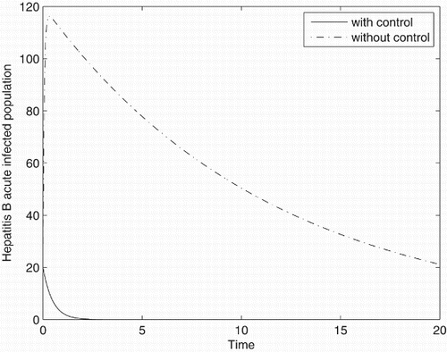
Figure 5. Population of hepatitis B chronically infected individuals with and without control.

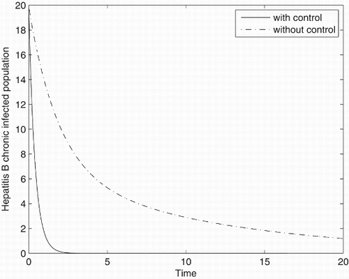
Figure 6. Population of recovered individuals with and without control.

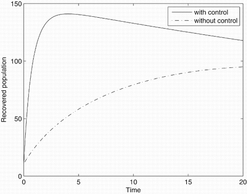
Figure 7. The plot shows the dynamic of control variable isolation.

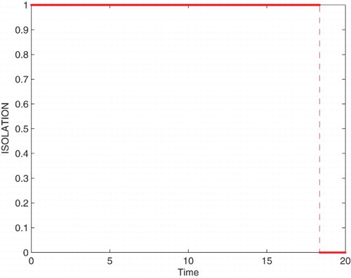
Figure 8. The plot shows the dynamic of control variable treatment.

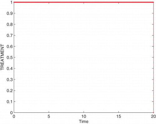
Figure 9. The plot shows the dynamic of control variable vaccination.

8. Conclusion

In this work, we presented the model for the transmission dynamic of acute and chronic HBV. We incorporated in the model acute-infected class and chronic-infected class and then developed the model with these new features. After formulating the model, we found the basic reproduction number $R_0$. As in epidemiological models, the model has two steady states, infected and uninfected steady states. Thus, we investigated both the states, disease-free state and endemic state and proved that the disease-free and endemic equilibria are both locally as well as globally stable under certain conditions. For the global stability, we developed the Lyapnovo function and showed that both the local and global dynamic are completely determined by the basic reproduction number $R_0$. Furthermore, three time-dependent control variables are taken and a control strategy for minimizing the number of infected individuals and maximizing the number of non-infected individuals was developed.

Finally, we presented the numerical simulation and verified all the analytical results numerically. By using control variables isolation, treatment and vaccination, we are able to control the spreading of hepatitis B. We believe that this new extension, assumption and analysis are biologically much more plausible.

Disclosure statement

No potential conflict of interest was reported by the authors.

Additional information

Funding

This work has been partially supported by Higher Education Commission (HEC) of Pakistan (project no. $20-1983/RandD/HEC/11$).

References

- R.M. Anderson and R.M. May, Infectious Disease of Humans, Dynamics and Control, Oxford University Press, Oxford, 1991.
- G. Birkhoff and G.C. Rota, Ordinary Differential Equation, 4th ed., John Wiley and Sons, New York, NY, 1989.
- M.H. Chang, Hepatitis virus infection, Semin. Fetal Neonatal Med. 12 (2007), pp. 160–167. doi: 10.1016/j.siny.2007.01.013
- CDC, Public Health Service inter-agency guidelines for screening donors of blood, plasma, organs, tissues, and semen for evidence of hepatitis B and hepatitis C, MMWR 40 (1991), pp. 1–17.
- I.K. Dontwi, W. Obeng-Denteh, L. Obin-Apraku and E.A. Andam, Modeling hepatitis B in a high prevalence district Ghana, Br. J. Math. Comput. Sci. 4 (2014), pp. 969–988. doi: 10.9734/BJMCS/2014/4682
- V.D. Driessche and P. Watmough, Reproduction numbers and sub threshold endemic equilibria for compartmental models of disease transmission, Math. Biosci. 180 (2002), pp. 29–48. doi: 10.1016/S0025-5564(02)00108-6
- A.V. Kamyad, R. Akbari, A.A. Heydari, and A. Heydari, Mathematical modeling of transmission dynamics and optimal control of vaccination and treatment for hepatitis B virus, Comput. Math. Methods Med. 475451 (2014), pp. 1–15. doi: 10.1155/2014/475451
- T. Khan, G. Zaman, and O. Algahtani, Transmission dynamic and vaccination of hepatitis B epidemic model, WULFENIA J. 22 (2015), pp. 230–241.
- J.P. LaSalle, The Stability of Dynamical Systems, SIAM, Philadelphia, PA, 1976.
- D. Lavanchy, Hepatitis B virus epidemiology, disease burden, treatment, and current and emerging prevention and control measures, J. Viral Hepat. 11 (2004), pp. 97–107. doi: 10.1046/j.1365-2893.2003.00487.x
- M.K. Libbus and L.M. phillips, Public health management of perinatal hepatitis B virus, Public Health Nurs. 26 (2009), pp. 353–361. doi: 10.1111/j.1525-1446.2009.00790.x
- A.S. Lok, E.J Heathcote, and J.H. Hoofnagle, Management of hepatitis B, 2000 – Summary of a workshop, Gastroenterology 120 (2001), pp. 1828–1853. doi: 10.1053/gast.2001.24839
- J. Mann and M. Roberts, Modelling the epidemiology of hepatitis B in New Zealand, J. Theor. Biol. 269 (2011), pp. 266–272. doi: 10.1016/j.jtbi.2010.10.028
- J.E. Maynard, M.A. Kane, and S.C. Hadler, Global control of hepatitis B through vaccination role of hepatitis B vaccine in the expanded programme on immunization, Rev. Infect. 2 (1989), pp. S574–S578. doi: 10.1093/clinids/11.Supplement_3.S574
- B.J. McMahon, Epidemiology and natural history of hepatitis B, Semin. Liver Dis. 25 (2005), pp. 3–8. doi: 10.1055/s-2005-915644
- G.F. Medley, N.A. Lindop, W.J. Edmunds, and D.J. Nokes, Hepatitis-B virus endemicity, heterogeneity, catastrophic dynamics and control, Nat. Med. 7 (2001), pp. 619–624. doi: 10.1038/87953
- J.R. Nokes, D.J. Medley, and G.F. Anderson, The transmission dynamics of hepatitis B in the UK: A mathematical model for evaluating costs and effectiveness of immunization programmes, Epidemiol. Infect. 116 (1996), pp. 71–89. doi: 10.1017/S0950268800058970
- J. Pang, J.-A. Cui, and X. Zhou, Dynamical behavior of a hepatitis B virus transmission model with vaccination, J. Theor. Biol. 265 (2010), pp. 572–578. doi: 10.1016/j.jtbi.2010.05.038
- C.W. Shepard, E.P. Simard, L. Finelli, A.E. Fiore, and B.P. Bell, Hepatitis B virus infection epidemiology and vaccination, Epidemiol. Rev. 28 (2006), pp. 112–125. doi: 10.1093/epirev/mxj009
- S. Thornley, C. Bullen, and M. Roberts, Hepatitis B in a high prevalence New Zealand population: A mathematical model applied to infection control policy, J. Theor. Biol. 254 (2008), pp. 599–603. doi: 10.1016/j.jtbi.2008.06.022
- J. Wang, J. Pang, and X. Liu, Modelling diseases with relapse and nonlinear incidence of infection: A multi-group epidemic model, J. Biol. Dyn. 8 (2014), pp. 99–116. doi: 10.1080/17513758.2014.912682
- J. Wang, R. Zhang, and T. Kuniya, The stability analysis of an SVEIR model with continuous age-structure in the exposed and infectious classes, J. Biol. Dyn. 9 (2015), pp. 73–101. doi: 10.1080/17513758.2015.1006696
- R. Williams, Global challenges in liver disease, Hepatology 44 (2006), pp. 521–526. doi: 10.1002/hep.21347
- G. Zaman, Y.H. Kang, and I.H. Jung, Stability and optimal vaccination of an SIR epidemic model, BioSystems 93 (2008), pp. 240–249. doi: 10.1016/j.biosystems.2008.05.004
- G. Zaman, Y.H. Kang, and I.H. Jung, Optimal treatment of an SIR epidemic model with time delay, BioSystems 98 (2009), pp. 43–50. doi: 10.1016/j.biosystems.2009.05.006
- S. Zhang and Y. Zhou, The analysis and application of an HBV model, Appl. Math. Model. 36 (2012), pp. 1302–1312. doi: 10.1016/j.apm.2011.07.087
- S.J. Zhao, Z.Y. Xu, and Y. Lu, A mathematical model of hepatitis B virus transmission and its application for vaccination strategy in China, Int. J. Epidemiol. 29 (2000), pp. 744–752. doi: 10.1093/ije/29.4.744