Stability of a binge drinking model with delay

ABSTRACT

A more realistic binge drinking model with time delay is introduced. Time delay is used to represent the time lag of the immunity against drinking in our model. For the model without the time delay, using Routh–Hurwitz criterion, we obtain that the alcohol-free equilibrium is locally asymptotically stable if $R_0<1$. We also obtain that the unique alcohol-present equilibrium is locally asymptotically stable if $R_0>1$. For the model with time delay, the local stability of all the equilibria is derived. Furthermore, regardless of the time delay length, using comparison theorem and iteration technique, we obtain that the alcohol-free equilibrium is globally asymptotically stable under certain conditions. Numerical simulations are also conducted to illustrate and extend our analytic results.

KEYWORDS:

• Binge drinking
• time delay
• stability
• equilibrium

1. Introduction

The drinking behaviours of people pose a significant public health concern. US surveys indicate that approximately 90% of college students have consumed alcohol at least once [7], and more than 40% of college students have engaged in binge drinking [9,20]. As we all know, excessive drinking is not only harmful to personal health, but also leads to a range of negative social effects such as violence, antisocial and criminal behaviour. Long-term alcoholism will produce negative change in the brain, such as tolerance and physical dependence. Alcohol damages almost all parts of the body and contributes to a number of human disease including live cirrhosis, pancreatitis, heart disease, sexual dysfunction and eventually death [1]. The growing excessive drinking increases the risk of breast cancer by 13% every year. In addition, there are data show that, on average, heavy drinker die 10-20 years earlier than nondrinkers. 40% and 32% of family divorce are caused by alcohol, in America and China, respectively [6,15,16]. The World Health Organization reports that the harmful use of alcohol causes approximately 3.3 million deaths every year(or 5.9% of all the global deaths), and 5.1% of the global burden of disease is attributable to alcohol consumption. Although there had been many attempts to reduce the problem, alcohol by young people had persisted and in some cases increased over the past several decades  [19]. Alcoholism is becoming more and more dangerous and serious as well as a widespread social phenomenon, so the study of alcoholism is an important aspect of social epidemic.

Mathematical models can mimic the process of drinking behaviour. Since the social interaction is considered to be the key factor in spreading the behaviour which can result in adverse health effects, alcoholism can be viewed as a treatable contagious disease. So far, several different mathematical models for drinking have been formulated and studied. Manthey et al. [10] built an epidemiological model to capture the dynamics of campus drinking. Their results showed that the reproductive numbers were not sufficient to predict whether drinking behaviour would persist on campus and that the pattern of recruiting new members played a significant role in the reduction of campus alcohol problems. Xiang et al.  [23] dealt with the global property of a drinking model with public health educational campaigns, and concluded that the public health educational campaigns of drinking individuals could slow down the drinking dynamics.

It is well known that taking into account the time delay effect is a typical approach for modelling oscillatory behaviour of population. Huo and Ma [4] developed a nonlinear alcoholism model with awareness programmes and time delay, they incorporated time delay $\tau >0$ during which a susceptible individual became a heavy drinker. They concluded that the time delay in alcohol consumption habit which developed in susceptible population might result in Hopf bifurcation by increasing the value of time delay. Wang et al. [18] formulated an alcohol quitting model in which they considered the impact of distributed time delay between contact and infection process by characterizing dynamic nature of alcoholism behaviours, and they generalized the infection rate to the general case. Furthermore they considered two control strategies, that is, education and treatment. Other models about drinking, smoking or epidemic can be found in [3,5,8,11–13,17,21,22,24,25].

Motivated by the above works, we set up a more realistic drinking model with two stages and time delay. We divide alcoholics into light problem alcoholics and heavy problem alcoholics, and incorporate time delay which describes the time lag of the ‘immunity’ against drinking in our model. Our goal is to study dynamics of our model. The remainder of this paper is organized as follows. In Section 2, we formulate our mathematical model. The existence of equilibria are obtained in Section 3. In Section 4, the stability of all the equilibria is studied. To support our theoretical results, some numerical simulations are included in Section 5. In Section 6, we give some conclusions and discussions.

2. The model formulation

Research Group of treatment and rehabilitation of the U.S. National Institute on Alcohol Abuse and Alcoholism (NIAAA), said that the daily alcohol consumption for men is not more than four standard volume (standard volume= 10 g of pure alcohol), women are not more than three standard volume. The ceiling of low-risk alcohol consumption per week is 14 standard volume for men, and 7 standard volume for women. If a person whose alcohol consumption is more than daily or weekly drinking ceiling, he/she most likely develop to abuse alcohol or addicted alcohol [14]. So we divide the whole population into four compartments: $S\left(t\right)$, $A\left(t\right)$, $I\left(t\right)$, $R\left(t\right)$. $S\left(t\right)$ denotes susceptible individuals who do not drink or only drink moderately. The light problem alcoholics, denoted by $A\left(t\right)$, refers to the drinkers who drink beyond daily or weekly ceiling a little. The heavy problem alcoholics, denoted by $I\left(t\right)$, refers to the drinkers who drink far exceeding daily and weekly ceiling. The recovered individuals, denoted by $R\left(t\right)$, refers to the people who quit problem drinking temporarily. The total number of population at time t is given by $N\left(t\right)=S\left(t\right)+A\left(t\right)+I\left(t\right)+R\left(t\right)$. The transfer diagram is shown in Figure 1.

Figure 1. Transfer diagram of the drinking model.

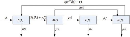
Figure 1 leads to the following drinking model with time delay: (1) $\begin{array}{rl}\frac{\mathrm{d}S\left(t\right)}{\mathrm{d}t}& =\mathrm{\Lambda }-S(\beta A+\gamma I)-\mu S+\eta {\mathrm{e}}^{-\mu \tau }R(t-\tau ),\\ \frac{\mathrm{d}A\left(t\right)}{\mathrm{d}t}& =S(\beta A+\gamma I)-pA-\mu A-mA,\\ \frac{\mathrm{d}I\left(t\right)}{\mathrm{d}t}& =pA-\delta I-\mu I,\\ \frac{\mathrm{d}R\left(t\right)}{\mathrm{d}t}& =\delta I+mA-\mu R-\eta {\mathrm{e}}^{-\mu \tau }R(t-\tau ).\end{array}$(1) where Λ is the recruitment rate of susceptible individuals who do not drink or drink only moderately. We assume that if a susceptible individual is infected by alcoholics, he will enter into light problem alcoholics. β is the transmission coefficient of infection for the susceptible individuals from the light problem alcoholics. γ is the transmission coefficient of infection for the susceptible individuals from the heavy problem alcoholics. A light problem alcoholic will become a heavy problem alcoholic at rate p due to excessive drinking. A light problem alcoholic will become a recovered individual at rate m due to treatment. A heavy problem alcoholic will become a recovered individual at rate δ due to treatment. A recuperator individual becomes a susceptible at rate η. We assume that all individuals' death rate is μ. $\eta {\mathrm{e}}^{-\mu \tau }R(t-\tau )$ represents that an individual has survived natural death in a recovery compartment before becoming susceptible again, where $\tau >0$ is a constant representing the time lag of the ‘immunity’ against drinking. η is the rate of losing ‘immunity’ against drinking, $\eta >0$ implies that the recovered individuals would lose the ‘immunity’, $\eta =0$ implies that the recovered individuals are with the permanent ‘immunity’. The parameters are all positive.

Suppose that the initial conditions for system (1(1) $\begin{array}{rl}\frac{\mathrm{d}S\left(t\right)}{\mathrm{d}t}& =\mathrm{\Lambda }-S(\beta A+\gamma I)-\mu S+\eta {\mathrm{e}}^{-\mu \tau }R(t-\tau ),\\ \frac{\mathrm{d}A\left(t\right)}{\mathrm{d}t}& =S(\beta A+\gamma I)-pA-\mu A-mA,\\ \frac{\mathrm{d}I\left(t\right)}{\mathrm{d}t}& =pA-\delta I-\mu I,\\ \frac{\mathrm{d}R\left(t\right)}{\mathrm{d}t}& =\delta I+mA-\mu R-\eta {\mathrm{e}}^{-\mu \tau }R(t-\tau ).\end{array}$(1) ) take the form (2) $\begin{array}{rl}S\left(\theta \right)& ={\phi }_1\left(\theta \right),A\left(\theta \right)={\phi }_2\left(\theta \right),I\left(\theta \right)={\phi }_3\left(\theta \right),R\left(\theta \right)={\phi }_4\left(\theta \right),\\ {\phi }_1& \ge 0,{\phi }_2\ge 0,{\phi }_3\ge 0,{\phi }_4\ge 0,\theta \in [-\tau ,0],\\ {\phi }_1\left(0\right)& >0,{\phi }_2\left(0\right)>0,{\phi }_3\left(0\right)>0,{\phi }_4\left(0\right)>0,\end{array}$(2) where $\mathrm{\Phi }=\left({\phi }_1\right(\theta ),{\phi }_2(\theta ),{\phi }_3(\theta ),{\phi }_4(\theta \left)\right)\in C\left(\right[-\tau ,0],R_{+}^4),$ the Banach space of continuous functions mapping the interval $[-\tau ,0]$ into $R_{+}^4,$ where $R_{+}^4=\left\{\right(x_1,x_2,x_3,x_4):x_i\ge 0,i=1,2,3,4\}.$

It is well known that system (1(1) $\begin{array}{rl}\frac{\mathrm{d}S\left(t\right)}{\mathrm{d}t}& =\mathrm{\Lambda }-S(\beta A+\gamma I)-\mu S+\eta {\mathrm{e}}^{-\mu \tau }R(t-\tau ),\\ \frac{\mathrm{d}A\left(t\right)}{\mathrm{d}t}& =S(\beta A+\gamma I)-pA-\mu A-mA,\\ \frac{\mathrm{d}I\left(t\right)}{\mathrm{d}t}& =pA-\delta I-\mu I,\\ \frac{\mathrm{d}R\left(t\right)}{\mathrm{d}t}& =\delta I+mA-\mu R-\eta {\mathrm{e}}^{-\mu \tau }R(t-\tau ).\end{array}$(1) ) has a unique solution $\left(S\right(t),A(t),I(t),R(t\left)\right)$ satisfying the initial conditions (2(2) $\begin{array}{rl}S\left(\theta \right)& ={\phi }_1\left(\theta \right),A\left(\theta \right)={\phi }_2\left(\theta \right),I\left(\theta \right)={\phi }_3\left(\theta \right),R\left(\theta \right)={\phi }_4\left(\theta \right),\\ {\phi }_1& \ge 0,{\phi }_2\ge 0,{\phi }_3\ge 0,{\phi }_4\ge 0,\theta \in [-\tau ,0],\\ {\phi }_1\left(0\right)& >0,{\phi }_2\left(0\right)>0,{\phi }_3\left(0\right)>0,{\phi }_4\left(0\right)>0,\end{array}$(2) ) by the fundamental theory of functional differential equations [2]. It is easy to show that all solutions of (1(1) $\begin{array}{rl}\frac{\mathrm{d}S\left(t\right)}{\mathrm{d}t}& =\mathrm{\Lambda }-S(\beta A+\gamma I)-\mu S+\eta {\mathrm{e}}^{-\mu \tau }R(t-\tau ),\\ \frac{\mathrm{d}A\left(t\right)}{\mathrm{d}t}& =S(\beta A+\gamma I)-pA-\mu A-mA,\\ \frac{\mathrm{d}I\left(t\right)}{\mathrm{d}t}& =pA-\delta I-\mu I,\\ \frac{\mathrm{d}R\left(t\right)}{\mathrm{d}t}& =\delta I+mA-\mu R-\eta {\mathrm{e}}^{-\mu \tau }R(t-\tau ).\end{array}$(1) ) with initial conditions (2(2) $\begin{array}{rl}S\left(\theta \right)& ={\phi }_1\left(\theta \right),A\left(\theta \right)={\phi }_2\left(\theta \right),I\left(\theta \right)={\phi }_3\left(\theta \right),R\left(\theta \right)={\phi }_4\left(\theta \right),\\ {\phi }_1& \ge 0,{\phi }_2\ge 0,{\phi }_3\ge 0,{\phi }_4\ge 0,\theta \in [-\tau ,0],\\ {\phi }_1\left(0\right)& >0,{\phi }_2\left(0\right)>0,{\phi }_3\left(0\right)>0,{\phi }_4\left(0\right)>0,\end{array}$(2) ) are defined on $[0,+\mathrm{\infty })$ and remain positive for all $t\ge 0$.

Using the fact that $N\left(t\right)=S\left(t\right)+A\left(t\right)+I\left(t\right)+R\left(t\right)$, system (1(1) $\begin{array}{rl}\frac{\mathrm{d}S\left(t\right)}{\mathrm{d}t}& =\mathrm{\Lambda }-S(\beta A+\gamma I)-\mu S+\eta {\mathrm{e}}^{-\mu \tau }R(t-\tau ),\\ \frac{\mathrm{d}A\left(t\right)}{\mathrm{d}t}& =S(\beta A+\gamma I)-pA-\mu A-mA,\\ \frac{\mathrm{d}I\left(t\right)}{\mathrm{d}t}& =pA-\delta I-\mu I,\\ \frac{\mathrm{d}R\left(t\right)}{\mathrm{d}t}& =\delta I+mA-\mu R-\eta {\mathrm{e}}^{-\mu \tau }R(t-\tau ).\end{array}$(1) ) is rewritten as (3) $\frac{\mathrm{d}N\left(t\right)}{\mathrm{d}t}=\mathrm{\Lambda }-\mu N\left(t\right),$(3) from Equation (3(3) $\frac{\mathrm{d}N\left(t\right)}{\mathrm{d}t}=\mathrm{\Lambda }-\mu N\left(t\right),$(3) ), we can obtain $N\left(t\right)=\frac{\mathrm{\Lambda }}{\mu }+c{\mathrm{e}}^{-\mu t}.$ So, $\underset{t\to +\mathrm{\infty }}{lim}N\left(t\right)=\mathrm{\Lambda }/\mu$. Hence, the feasible region of system (1(1) $\begin{array}{rl}\frac{\mathrm{d}S\left(t\right)}{\mathrm{d}t}& =\mathrm{\Lambda }-S(\beta A+\gamma I)-\mu S+\eta {\mathrm{e}}^{-\mu \tau }R(t-\tau ),\\ \frac{\mathrm{d}A\left(t\right)}{\mathrm{d}t}& =S(\beta A+\gamma I)-pA-\mu A-mA,\\ \frac{\mathrm{d}I\left(t\right)}{\mathrm{d}t}& =pA-\delta I-\mu I,\\ \frac{\mathrm{d}R\left(t\right)}{\mathrm{d}t}& =\delta I+mA-\mu R-\eta {\mathrm{e}}^{-\mu \tau }R(t-\tau ).\end{array}$(1) ) is given by the set $\mathrm{\Omega }=\left\{\right(S,A,I,R)\in R_{+}^4:S+A+I+R⩽\frac{\mathrm{\Lambda }}{\mu }\},$ which is positively invariant with respect to system (1(1) $\begin{array}{rl}\frac{\mathrm{d}S\left(t\right)}{\mathrm{d}t}& =\mathrm{\Lambda }-S(\beta A+\gamma I)-\mu S+\eta {\mathrm{e}}^{-\mu \tau }R(t-\tau ),\\ \frac{\mathrm{d}A\left(t\right)}{\mathrm{d}t}& =S(\beta A+\gamma I)-pA-\mu A-mA,\\ \frac{\mathrm{d}I\left(t\right)}{\mathrm{d}t}& =pA-\delta I-\mu I,\\ \frac{\mathrm{d}R\left(t\right)}{\mathrm{d}t}& =\delta I+mA-\mu R-\eta {\mathrm{e}}^{-\mu \tau }R(t-\tau ).\end{array}$(1) ). We will consider dynamic behaviour of system (1(1) $\begin{array}{rl}\frac{\mathrm{d}S\left(t\right)}{\mathrm{d}t}& =\mathrm{\Lambda }-S(\beta A+\gamma I)-\mu S+\eta {\mathrm{e}}^{-\mu \tau }R(t-\tau ),\\ \frac{\mathrm{d}A\left(t\right)}{\mathrm{d}t}& =S(\beta A+\gamma I)-pA-\mu A-mA,\\ \frac{\mathrm{d}I\left(t\right)}{\mathrm{d}t}& =pA-\delta I-\mu I,\\ \frac{\mathrm{d}R\left(t\right)}{\mathrm{d}t}& =\delta I+mA-\mu R-\eta {\mathrm{e}}^{-\mu \tau }R(t-\tau ).\end{array}$(1) ) on the set Ω.

3. Existence of equilibria

According to the condition of system (1(1) $\begin{array}{rl}\frac{\mathrm{d}S\left(t\right)}{\mathrm{d}t}& =\mathrm{\Lambda }-S(\beta A+\gamma I)-\mu S+\eta {\mathrm{e}}^{-\mu \tau }R(t-\tau ),\\ \frac{\mathrm{d}A\left(t\right)}{\mathrm{d}t}& =S(\beta A+\gamma I)-pA-\mu A-mA,\\ \frac{\mathrm{d}I\left(t\right)}{\mathrm{d}t}& =pA-\delta I-\mu I,\\ \frac{\mathrm{d}R\left(t\right)}{\mathrm{d}t}& =\delta I+mA-\mu R-\eta {\mathrm{e}}^{-\mu \tau }R(t-\tau ).\end{array}$(1) ) has a unique alcohol-present equilibrium, we can define the value of the basic reproductive number $R_0$ as follows: (4) $R_0=\frac{\left[\beta \right(\mu +\delta )+p\gamma ]\mathrm{\Lambda }}{\mu (\mu +\delta )(\mu +m+p)}.$(4) It is easy to know the following theorem.

Theorem 3.1

System (1(1) $\begin{array}{rl}\frac{\mathrm{d}S\left(t\right)}{\mathrm{d}t}& =\mathrm{\Lambda }-S(\beta A+\gamma I)-\mu S+\eta {\mathrm{e}}^{-\mu \tau }R(t-\tau ),\\ \frac{\mathrm{d}A\left(t\right)}{\mathrm{d}t}& =S(\beta A+\gamma I)-pA-\mu A-mA,\\ \frac{\mathrm{d}I\left(t\right)}{\mathrm{d}t}& =pA-\delta I-\mu I,\\ \frac{\mathrm{d}R\left(t\right)}{\mathrm{d}t}& =\delta I+mA-\mu R-\eta {\mathrm{e}}^{-\mu \tau }R(t-\tau ).\end{array}$(1) ) always has the alcohol-free equilibrium $E_0=(\mathrm{\Lambda }/\mu ,0,0,0)$. Furthermore, system (1(1) $\begin{array}{rl}\frac{\mathrm{d}S\left(t\right)}{\mathrm{d}t}& =\mathrm{\Lambda }-S(\beta A+\gamma I)-\mu S+\eta {\mathrm{e}}^{-\mu \tau }R(t-\tau ),\\ \frac{\mathrm{d}A\left(t\right)}{\mathrm{d}t}& =S(\beta A+\gamma I)-pA-\mu A-mA,\\ \frac{\mathrm{d}I\left(t\right)}{\mathrm{d}t}& =pA-\delta I-\mu I,\\ \frac{\mathrm{d}R\left(t\right)}{\mathrm{d}t}& =\delta I+mA-\mu R-\eta {\mathrm{e}}^{-\mu \tau }R(t-\tau ).\end{array}$(1) ) has a unique alcohol-present equilibrium $E^{\ast }=(S^{\ast },A^{\ast },I^{\ast },R^{\ast })$ regardless of the time delay length if $R_0>1$.

Proof.

It is easy to see that the alcohol-free equilibrium $E_0=(\frac{\mathrm{\Lambda }}{\mu },0,0,0)$ always exists. From the third equation of Equation (1(1) $\begin{array}{rl}\frac{\mathrm{d}S\left(t\right)}{\mathrm{d}t}& =\mathrm{\Lambda }-S(\beta A+\gamma I)-\mu S+\eta {\mathrm{e}}^{-\mu \tau }R(t-\tau ),\\ \frac{\mathrm{d}A\left(t\right)}{\mathrm{d}t}& =S(\beta A+\gamma I)-pA-\mu A-mA,\\ \frac{\mathrm{d}I\left(t\right)}{\mathrm{d}t}& =pA-\delta I-\mu I,\\ \frac{\mathrm{d}R\left(t\right)}{\mathrm{d}t}& =\delta I+mA-\mu R-\eta {\mathrm{e}}^{-\mu \tau }R(t-\tau ).\end{array}$(1) ), let the right-hand side equal to zero, we have (5) $A^{\ast }=\frac{\mu +\delta }{p}{I}^{\ast }.$(5)

Using the fourth equation of Equations (1(1) $\begin{array}{rl}\frac{\mathrm{d}S\left(t\right)}{\mathrm{d}t}& =\mathrm{\Lambda }-S(\beta A+\gamma I)-\mu S+\eta {\mathrm{e}}^{-\mu \tau }R(t-\tau ),\\ \frac{\mathrm{d}A\left(t\right)}{\mathrm{d}t}& =S(\beta A+\gamma I)-pA-\mu A-mA,\\ \frac{\mathrm{d}I\left(t\right)}{\mathrm{d}t}& =pA-\delta I-\mu I,\\ \frac{\mathrm{d}R\left(t\right)}{\mathrm{d}t}& =\delta I+mA-\mu R-\eta {\mathrm{e}}^{-\mu \tau }R(t-\tau ).\end{array}$(1) ) and (5(5) $A^{\ast }=\frac{\mu +\delta }{p}{I}^{\ast }.$(5) ), $R^{\ast }$ can be written as (6) $R^{\ast }=\frac{[p\delta +m(\mu +\delta \left)\right]I^{\ast }}{p(\mu +\eta {\mathrm{e}}^{-\mu \tau })}.$(6)

Together the first and the second equations of Equation (1(1) $\begin{array}{rl}\frac{\mathrm{d}S\left(t\right)}{\mathrm{d}t}& =\mathrm{\Lambda }-S(\beta A+\gamma I)-\mu S+\eta {\mathrm{e}}^{-\mu \tau }R(t-\tau ),\\ \frac{\mathrm{d}A\left(t\right)}{\mathrm{d}t}& =S(\beta A+\gamma I)-pA-\mu A-mA,\\ \frac{\mathrm{d}I\left(t\right)}{\mathrm{d}t}& =pA-\delta I-\mu I,\\ \frac{\mathrm{d}R\left(t\right)}{\mathrm{d}t}& =\delta I+mA-\mu R-\eta {\mathrm{e}}^{-\mu \tau }R(t-\tau ).\end{array}$(1) ), using Equations (5(5) $A^{\ast }=\frac{\mu +\delta }{p}{I}^{\ast }.$(5) ) and (6(6) $R^{\ast }=\frac{[p\delta +m(\mu +\delta \left)\right]I^{\ast }}{p(\mu +\eta {\mathrm{e}}^{-\mu \tau })}.$(6) ), we obtain (7) $I^{\ast }=\frac{\mathrm{\Lambda }-\mu S^{\ast }}{\frac{(\mu +\delta )(\mu +p+m)}{p}-\frac{[p\delta +m(\mu +\delta \left)\right]\eta {\mathrm{e}}^{-\mu \tau }}{p(\mu +\eta {\mathrm{e}}^{-\mu \tau })}}.$(7)

Using the second equation of Equations (1(1) $\begin{array}{rl}\frac{\mathrm{d}S\left(t\right)}{\mathrm{d}t}& =\mathrm{\Lambda }-S(\beta A+\gamma I)-\mu S+\eta {\mathrm{e}}^{-\mu \tau }R(t-\tau ),\\ \frac{\mathrm{d}A\left(t\right)}{\mathrm{d}t}& =S(\beta A+\gamma I)-pA-\mu A-mA,\\ \frac{\mathrm{d}I\left(t\right)}{\mathrm{d}t}& =pA-\delta I-\mu I,\\ \frac{\mathrm{d}R\left(t\right)}{\mathrm{d}t}& =\delta I+mA-\mu R-\eta {\mathrm{e}}^{-\mu \tau }R(t-\tau ).\end{array}$(1) ) and (5(5) $A^{\ast }=\frac{\mu +\delta }{p}{I}^{\ast }.$(5) ), $S^{\ast }$ can be written as (8) $S^{\ast }=\frac{(\mu +\delta )(\mu +p+m)}{\beta (\mu +\delta )+p\gamma }.$(8)

If $R_0>1$, then $\mathrm{\Lambda }-\mu S^{\ast }>0$, so $I^{\ast }>0$. Hence, if $R_0>1$ system (1(1) $\begin{array}{rl}\frac{\mathrm{d}S\left(t\right)}{\mathrm{d}t}& =\mathrm{\Lambda }-S(\beta A+\gamma I)-\mu S+\eta {\mathrm{e}}^{-\mu \tau }R(t-\tau ),\\ \frac{\mathrm{d}A\left(t\right)}{\mathrm{d}t}& =S(\beta A+\gamma I)-pA-\mu A-mA,\\ \frac{\mathrm{d}I\left(t\right)}{\mathrm{d}t}& =pA-\delta I-\mu I,\\ \frac{\mathrm{d}R\left(t\right)}{\mathrm{d}t}& =\delta I+mA-\mu R-\eta {\mathrm{e}}^{-\mu \tau }R(t-\tau ).\end{array}$(1) ) has a unique endemic equilibrium $E^{\ast }=(S^{\ast },A^{\ast },I^{\ast },R^{\ast })$ regardless of the time delay length.

4. Stability analysis of equilibria

4.1. Stability analysis of equilibria With $\tau =0$

Theorem 4.1

The alcohol-free equilibrium $E_0$ of system (1(1) $\begin{array}{rl}\frac{\mathrm{d}S\left(t\right)}{\mathrm{d}t}& =\mathrm{\Lambda }-S(\beta A+\gamma I)-\mu S+\eta {\mathrm{e}}^{-\mu \tau }R(t-\tau ),\\ \frac{\mathrm{d}A\left(t\right)}{\mathrm{d}t}& =S(\beta A+\gamma I)-pA-\mu A-mA,\\ \frac{\mathrm{d}I\left(t\right)}{\mathrm{d}t}& =pA-\delta I-\mu I,\\ \frac{\mathrm{d}R\left(t\right)}{\mathrm{d}t}& =\delta I+mA-\mu R-\eta {\mathrm{e}}^{-\mu \tau }R(t-\tau ).\end{array}$(1) ) with $\tau =0$ is local asymptotically stable if $R_0<1$.

Proof.

The characteristic matrix of system (1(1) $\begin{array}{rl}\frac{\mathrm{d}S\left(t\right)}{\mathrm{d}t}& =\mathrm{\Lambda }-S(\beta A+\gamma I)-\mu S+\eta {\mathrm{e}}^{-\mu \tau }R(t-\tau ),\\ \frac{\mathrm{d}A\left(t\right)}{\mathrm{d}t}& =S(\beta A+\gamma I)-pA-\mu A-mA,\\ \frac{\mathrm{d}I\left(t\right)}{\mathrm{d}t}& =pA-\delta I-\mu I,\\ \frac{\mathrm{d}R\left(t\right)}{\mathrm{d}t}& =\delta I+mA-\mu R-\eta {\mathrm{e}}^{-\mu \tau }R(t-\tau ).\end{array}$(1) ) is as follows: (9) $\begin{array}{r}\left[\begin{array}{cccc}\lambda +(\beta \overline{A}+\gamma \overline{I})+\mu & \beta \overline{S}& \gamma \overline{S}& -\eta {\mathrm{e}}^{-(\lambda +\mu )\tau }\\ -(\beta \overline{A}+\gamma \overline{I})& \lambda -\beta \overline{S}+p+m+\mu & -\gamma \overline{S}& 0\\ 0& -p& \lambda +\mu +\delta & 0\\ 0& -m& -\delta & \lambda +\mu +\eta {\mathrm{e}}^{-(\lambda +\mu )\tau }\end{array}\right],\end{array}$(9) where $(\overline{S},\overline{A},\overline{I},\overline{R})$ denotes any equilibrium of Equation (1(1) $\begin{array}{rl}\frac{\mathrm{d}S\left(t\right)}{\mathrm{d}t}& =\mathrm{\Lambda }-S(\beta A+\gamma I)-\mu S+\eta {\mathrm{e}}^{-\mu \tau }R(t-\tau ),\\ \frac{\mathrm{d}A\left(t\right)}{\mathrm{d}t}& =S(\beta A+\gamma I)-pA-\mu A-mA,\\ \frac{\mathrm{d}I\left(t\right)}{\mathrm{d}t}& =pA-\delta I-\mu I,\\ \frac{\mathrm{d}R\left(t\right)}{\mathrm{d}t}& =\delta I+mA-\mu R-\eta {\mathrm{e}}^{-\mu \tau }R(t-\tau ).\end{array}$(1) ). The associated transcendental characteristic equation of (9(9) $\begin{array}{r}\left[\begin{array}{cccc}\lambda +(\beta \overline{A}+\gamma \overline{I})+\mu & \beta \overline{S}& \gamma \overline{S}& -\eta {\mathrm{e}}^{-(\lambda +\mu )\tau }\\ -(\beta \overline{A}+\gamma \overline{I})& \lambda -\beta \overline{S}+p+m+\mu & -\gamma \overline{S}& 0\\ 0& -p& \lambda +\mu +\delta & 0\\ 0& -m& -\delta & \lambda +\mu +\eta {\mathrm{e}}^{-(\lambda +\mu )\tau }\end{array}\right],\end{array}$(9) ) is given by (10) $\begin{array}{rl}-\eta & {\mathrm{e}}^{-(\lambda +\mu )\tau }(\beta \overline{A}+\gamma \overline{I})(p\delta +(\lambda +\mu +\delta \left)m\right)+(\lambda +\mu +\eta {\mathrm{e}}^{-(\lambda +\mu )\tau })\\ & \left[\right(\lambda +\mu +\beta \overline{A}+\gamma \overline{I}\left)\right((\lambda +\mu +p+m-\beta \overline{S})(\lambda +\mu +\delta )-p\gamma \overline{S})\\ & +(\beta \overline{A}+\gamma \overline{I})\left(\beta \overline{S}\right(\lambda +\mu +\delta )+p\gamma \overline{S})]=0.\end{array}$(10) It is clear that the associated transcendental characteristic equation of (10(10) $\begin{array}{rl}-\eta & {\mathrm{e}}^{-(\lambda +\mu )\tau }(\beta \overline{A}+\gamma \overline{I})(p\delta +(\lambda +\mu +\delta \left)m\right)+(\lambda +\mu +\eta {\mathrm{e}}^{-(\lambda +\mu )\tau })\\ & \left[\right(\lambda +\mu +\beta \overline{A}+\gamma \overline{I}\left)\right((\lambda +\mu +p+m-\beta \overline{S})(\lambda +\mu +\delta )-p\gamma \overline{S})\\ & +(\beta \overline{A}+\gamma \overline{I})\left(\beta \overline{S}\right(\lambda +\mu +\delta )+p\gamma \overline{S})]=0.\end{array}$(10) ) at $E_0=(\mathrm{\Lambda }/\mu ,0,0,0)=(\overline{S},\overline{A},\overline{I},\overline{R})$ becomes (11) $(\lambda +\mu )(\lambda +\mu +\eta {\mathrm{e}}^{-(\lambda +\mu )\tau })\left[\right(\lambda -\beta \frac{\mathrm{\Lambda }}{\mu }+\mu +p+m\left)\right(\lambda +\mu +\delta )-p\gamma \frac{\mathrm{\Lambda }}{\mu }]=0.$(11) For $\tau =0$, Equation (11(11) $(\lambda +\mu )(\lambda +\mu +\eta {\mathrm{e}}^{-(\lambda +\mu )\tau })\left[\right(\lambda -\beta \frac{\mathrm{\Lambda }}{\mu }+\mu +p+m\left)\right(\lambda +\mu +\delta )-p\gamma \frac{\mathrm{\Lambda }}{\mu }]=0.$(11) ) can be written as (12) $\begin{array}{rl}& (\lambda +\mu )(\lambda +\mu +\eta )[{\lambda }^2+(\mu +p+m+\mu +\delta -\beta \frac{\mathrm{\Lambda }}{\mu })\lambda \\ & +(\mu +\delta )(\mu +p+m-\beta \frac{\mathrm{\Lambda }}{\mu })-p\gamma \frac{\mathrm{\Lambda }}{\mu }]=0.\end{array}$(12) We can obtain the characteristic roots are $\lambda =-\mu ,\lambda =-(\mu +\eta )$, and roots of the following equation: (13) ${\lambda }^2+(\mu +p+m+\mu +\delta -\beta \frac{\mathrm{\Lambda }}{\mu })\lambda +(\mu +\delta )(\mu +p+m-\beta \frac{\mathrm{\Lambda }}{\mu })-p\gamma \frac{\mathrm{\Lambda }}{\mu }=0.$(13) If $R_0<1$, we have $\left[\beta \right(\mu +\delta )+p\gamma ]\left(\mathrm{\Lambda }/\mu \right)<(\mu +\delta )(\mu +m+p)$, then, $\begin{array}{rl}& \mu +p+m+\mu +\delta -\beta \frac{\mathrm{\Lambda }}{\mu }>0,\\ & (\mu +\delta )(\mu +p+m-\beta \frac{\mathrm{\Lambda }}{\mu })-p\gamma \frac{\mathrm{\Lambda }}{\mu }>0.\end{array}$ The real parts of all eigenvalues of $E_0$ are negative. Thus, the alcohol-free equilibrium $E_0$ of system (1(1) $\begin{array}{rl}\frac{\mathrm{d}S\left(t\right)}{\mathrm{d}t}& =\mathrm{\Lambda }-S(\beta A+\gamma I)-\mu S+\eta {\mathrm{e}}^{-\mu \tau }R(t-\tau ),\\ \frac{\mathrm{d}A\left(t\right)}{\mathrm{d}t}& =S(\beta A+\gamma I)-pA-\mu A-mA,\\ \frac{\mathrm{d}I\left(t\right)}{\mathrm{d}t}& =pA-\delta I-\mu I,\\ \frac{\mathrm{d}R\left(t\right)}{\mathrm{d}t}& =\delta I+mA-\mu R-\eta {\mathrm{e}}^{-\mu \tau }R(t-\tau ).\end{array}$(1) ) with $\tau =0$ is local asymptotically stable.

Next, we turn to consider the local stability of the alcohol-present equilibrium $E^{\ast }$ with $\tau =0$.

Theorem 4.2

If $R_0>1,$ the alcohol-present equilibrium $E^{\ast }$ of the system (1(1) $\begin{array}{rl}\frac{\mathrm{d}S\left(t\right)}{\mathrm{d}t}& =\mathrm{\Lambda }-S(\beta A+\gamma I)-\mu S+\eta {\mathrm{e}}^{-\mu \tau }R(t-\tau ),\\ \frac{\mathrm{d}A\left(t\right)}{\mathrm{d}t}& =S(\beta A+\gamma I)-pA-\mu A-mA,\\ \frac{\mathrm{d}I\left(t\right)}{\mathrm{d}t}& =pA-\delta I-\mu I,\\ \frac{\mathrm{d}R\left(t\right)}{\mathrm{d}t}& =\delta I+mA-\mu R-\eta {\mathrm{e}}^{-\mu \tau }R(t-\tau ).\end{array}$(1) ) with $\tau =0$ is local asymptotically stable.

Proof.

The characteristic equation of (10(10) $\begin{array}{rl}-\eta & {\mathrm{e}}^{-(\lambda +\mu )\tau }(\beta \overline{A}+\gamma \overline{I})(p\delta +(\lambda +\mu +\delta \left)m\right)+(\lambda +\mu +\eta {\mathrm{e}}^{-(\lambda +\mu )\tau })\\ & \left[\right(\lambda +\mu +\beta \overline{A}+\gamma \overline{I}\left)\right((\lambda +\mu +p+m-\beta \overline{S})(\lambda +\mu +\delta )-p\gamma \overline{S})\\ & +(\beta \overline{A}+\gamma \overline{I})\left(\beta \overline{S}\right(\lambda +\mu +\delta )+p\gamma \overline{S})]=0.\end{array}$(10) ) at $E^{\ast }$ is (14) ${\lambda }^4+a_1{\lambda }^3+a_2{\lambda }^2+a_3\lambda +a_4=(b_1{\lambda }^3+b_2{\lambda }^2+b_3\lambda +b_4).$(14) where $\begin{array}{rl}{a}_1& =4\mu +m+p+\delta +\beta A^{\ast }+\gamma I^{\ast }-\beta S^{\ast },\\ a_2& =\mu (2\mu +p+m+\delta -\beta S^{\ast })+(\beta A^{\ast }+\gamma I^{\ast })(2\mu +p+m+\delta )\\ & +\mu (3\mu +p+m+\delta -\beta S^{\ast }+\beta A^{\ast }+\gamma I^{\ast }),\\ a_3& =(\beta A^{\ast }+\gamma I^{\ast })(\mu +m+p)(\mu +\delta )+{\mu }^2(2\mu +p+m+\delta -\beta S^{\ast })\\ & +\mu (\beta A^{\ast }+\gamma I^{\ast })(2\mu +p+m+\delta ),\\ a_4& =\mu (\beta A^{\ast }+\gamma I^{\ast })(\mu +m+p)(\mu +\delta ),\\ b_1& =-\eta ,\\ b_2& =-\eta (3\mu +m+p+\delta +\beta A^{\ast }+\gamma I^{\ast }-\beta S^{\ast }),\\ b_3& =-\eta \left[\mu \right(2\mu +p+m+\delta -\beta S^{\ast }\left)+\right(\beta A^{\ast }+\gamma I^{\ast }\left)\right(2\mu +p+m+\delta \left)-\right(\beta A^{\ast }+\gamma I^{\ast }\left)m\right],\\ b_4& =-\eta \left[\right(\beta A^{\ast }+\gamma I^{\ast }\left)\right(\mu +m+p\left)\right(\mu +\delta \left)-\right(\beta A^{\ast }+\gamma I^{\ast }\left)p\delta -\right(\beta A^{\ast }+\gamma I^{\ast }\left)\right(\mu +\delta \left)m\right].\end{array}$ Since $(\mu +\delta )(\mu +p+m)=\left[\beta \right(\mu +\delta )+p\gamma ]S^{\ast }$, then $\mu +p+m>\beta S^{\ast }$. It is easy to see $a_i>0,b_i<0$ $(i=1,2,3,4)$.

Let $B=3\mu +m+p+\delta +\beta A^{\ast }+\gamma I^{\ast }-\beta S^{\ast },C=2\mu +p+m+\delta -\beta S^{\ast }$, we have $\begin{array}{rl}{H}_1& =a_1-b_1=4\mu +m+p+\delta +\beta A^{\ast }+\gamma I^{\ast }-\beta S^{\ast }+\eta >0,\\ H_2& =(a_1-b_1)(a_2-b_2)-(a_3-b_3)=B^2(\mu +\eta )+\mu BC+(\mu +\eta {)}^{2}B+\\ & B(\beta A^{\ast }+\gamma I^{\ast })(2\mu +p+m+\delta )\\ & -(\beta A^{\ast }+\gamma I^{\ast })(\mu +m+p)(\mu +\delta )+m\eta (\beta A^{\ast }+\gamma I^{\ast })>0,\\ H_3=& (a_3-b_3)\left[\right(a_1-b_1\left)\right(a_2-b_2)-(a_3-b_3\left)\right]-(a_1-b_1{)}^2(a_4-b_4),\\ H_4=& (a_4-b_4)H_3.\end{array}$ By complex calculations, we also can get $H_3>0$, $H_4>0$.

Thus, by using the Routh–Hurwitz criterion, we obtain that all the eigenvalues of Equation (14(14) ${\lambda }^4+a_1{\lambda }^3+a_2{\lambda }^2+a_3\lambda +a_4=(b_1{\lambda }^3+b_2{\lambda }^2+b_3\lambda +b_4).$(14) ) have negative real parts. Hence, if $R_0>1$, the alcohol-present equilibrium $E^{\ast }$ of the system (1(1) $\begin{array}{rl}\frac{\mathrm{d}S\left(t\right)}{\mathrm{d}t}& =\mathrm{\Lambda }-S(\beta A+\gamma I)-\mu S+\eta {\mathrm{e}}^{-\mu \tau }R(t-\tau ),\\ \frac{\mathrm{d}A\left(t\right)}{\mathrm{d}t}& =S(\beta A+\gamma I)-pA-\mu A-mA,\\ \frac{\mathrm{d}I\left(t\right)}{\mathrm{d}t}& =pA-\delta I-\mu I,\\ \frac{\mathrm{d}R\left(t\right)}{\mathrm{d}t}& =\delta I+mA-\mu R-\eta {\mathrm{e}}^{-\mu \tau }R(t-\tau ).\end{array}$(1) ) with $\tau =0$ is local asymptotically stable.

4.2. Stability analysis of equilibria with $\tau >0$

Theorem 4.3

If $R_0<1$ and $\mu ⩾\eta {\mathrm{e}}^{-\mu \tau },$ the alcohol-free equilibrium $E_0$ of system (1(1) $\begin{array}{rl}\frac{\mathrm{d}S\left(t\right)}{\mathrm{d}t}& =\mathrm{\Lambda }-S(\beta A+\gamma I)-\mu S+\eta {\mathrm{e}}^{-\mu \tau }R(t-\tau ),\\ \frac{\mathrm{d}A\left(t\right)}{\mathrm{d}t}& =S(\beta A+\gamma I)-pA-\mu A-mA,\\ \frac{\mathrm{d}I\left(t\right)}{\mathrm{d}t}& =pA-\delta I-\mu I,\\ \frac{\mathrm{d}R\left(t\right)}{\mathrm{d}t}& =\delta I+mA-\mu R-\eta {\mathrm{e}}^{-\mu \tau }R(t-\tau ).\end{array}$(1) ) with $\tau >0$ is local asymptotically stable.

Proof.

Linearizing the system (1(1) $\begin{array}{rl}\frac{\mathrm{d}S\left(t\right)}{\mathrm{d}t}& =\mathrm{\Lambda }-S(\beta A+\gamma I)-\mu S+\eta {\mathrm{e}}^{-\mu \tau }R(t-\tau ),\\ \frac{\mathrm{d}A\left(t\right)}{\mathrm{d}t}& =S(\beta A+\gamma I)-pA-\mu A-mA,\\ \frac{\mathrm{d}I\left(t\right)}{\mathrm{d}t}& =pA-\delta I-\mu I,\\ \frac{\mathrm{d}R\left(t\right)}{\mathrm{d}t}& =\delta I+mA-\mu R-\eta {\mathrm{e}}^{-\mu \tau }R(t-\tau ).\end{array}$(1) ) with $\tau >0$ around $E_0$ we can obtain the characteristic roots are $\lambda =-\mu$ and roots of the following: (15) ${\lambda }^3+a_{11}{\lambda }^2+a_{21}\lambda +a_{31}=(b_{11}{\lambda }^2+b_{21}\lambda +b_{31}){\mathrm{e}}^{-\lambda \tau }.$(15) where $\begin{array}{rl}{a}_{11}& =3\mu +m+p+\delta -\beta \frac{\mathrm{\Lambda }}{\mu },\\ a_{21}& =\mu (2\mu +p+m+\delta -\beta \frac{\mathrm{\Lambda }}{\mu })+(\mu +\delta )(\mu +p+m)(1-R_0),\\ a_{31}& =\mu (\mu +p+m)(\mu +\delta )(1-R_0),\\ b_{11}& =-\eta {\mathrm{e}}^{-\mu \tau },\\ b_{21}& =-\eta {\mathrm{e}}^{-\mu \tau }(2\mu +m+p+\delta -\beta \frac{\mathrm{\Lambda }}{\mu }),\\ b_{31}& =-\eta {\mathrm{e}}^{-\mu \tau }(\mu +p+m)(\mu +\delta )(1-R_0).\end{array}$ If $R_0<1$, it is easy to see $a_{i1}>0,b_{i1}<0(i=1,2,3,4)$. Then Equation (15(15) ${\lambda }^3+a_{11}{\lambda }^2+a_{21}\lambda +a_{31}=(b_{11}{\lambda }^2+b_{21}\lambda +b_{31}){\mathrm{e}}^{-\lambda \tau }.$(15) ) does not have non-negative real solutions. Now we consider whether Equation (15(15) ${\lambda }^3+a_{11}{\lambda }^2+a_{21}\lambda +a_{31}=(b_{11}{\lambda }^2+b_{21}\lambda +b_{31}){\mathrm{e}}^{-\lambda \tau }.$(15) ) has purely imaginary solutions or not.

Suppose $\lambda =\omega \mathrm{i}(\omega >0)$ is a root of Equation (15(15) ${\lambda }^3+a_{11}{\lambda }^2+a_{21}\lambda +a_{31}=(b_{11}{\lambda }^2+b_{21}\lambda +b_{31}){\mathrm{e}}^{-\lambda \tau }.$(15) ). Then we have (16) $-{\omega }^3\mathrm{i}-a_{11}{\omega }^2+a_{21}\omega \mathrm{i}+a_{31}=(\cos \omega \tau -\mathrm{i}\sin \omega \tau )(-b_{11}{\omega }^2+b_{21}\omega \mathrm{i}+b_{31}).$(16) Separating the real and imaginary parts, we have the following system: (17) $\begin{array}{rl}-{\omega }^3+a_{21}\omega & =b_{21}\omega \cos \omega \tau -\sin \omega \tau (b_{31}-b_{11}{\omega }^2),\end{array}$(17) (18) $\begin{array}{rl}-a_{11}{\omega }^2+a_{31}& =(b_{31}-b_{11}{\omega }^2)\cos \omega \tau +b_{21}\omega \sin \omega \tau .\end{array}$(18) To eliminate the trigonometric functions we square both sides of each equation above and we add the squared equations (17(17) $\begin{array}{rl}-{\omega }^3+a_{21}\omega & =b_{21}\omega \cos \omega \tau -\sin \omega \tau (b_{31}-b_{11}{\omega }^2),\end{array}$(17) ) and (18(18) $\begin{array}{rl}-a_{11}{\omega }^2+a_{31}& =(b_{31}-b_{11}{\omega }^2)\cos \omega \tau +b_{21}\omega \sin \omega \tau .\end{array}$(18) ) to obtain the following equation: (19) $(-{\omega }^3+a_{21}\omega {)}^2+(-a_{11}{\omega }^2+a_{31}{)}^2=(b_{21}\omega {)}^2+(b_{31}-b_{11}{\omega }^2{)}^2,$(19) i.e. (20) ${\omega }^6+(a_{11}^2-2a_{21}-b_{11}^2){\omega }^4+(a_{21}^2-2a_{11}{a}_{31}-b_{21}^2+2b_{11}{b}_{31}){\omega }^2+a_{31}^2-b_{31}^2=0.$(20) Let $e={\omega }^2$, we obtain (21) $e^3+d_{11}{e}^2+d_{21}e+d_{31}=0,$(21) where $\begin{array}{rl}{d}_{11}& =a_{11}^2-2a_{21}-b_{11}^2={(3\mu +m+p+\delta +\beta \frac{\mathrm{\Lambda }}{\mu })}^2-2\mu (2\mu +p+m+\delta -\beta \frac{\mathrm{\Lambda }}{\mu })\\ & -2(\mu +\delta )(\mu +p+m)(1-R_0)-{\eta }^2{\mathrm{e}}^{-2\mu \tau },\\ d_{21}& =a_{21}^2-2a_{11}{a}_{31}-b_{21}^2+2b_{11}{b}_{31}=({\mu }^2-{\eta }^2{\mathrm{e}}^{-2\mu \tau })\\ & \times [{(2\mu +p+m+\delta -\beta \frac{\mathrm{\Lambda }}{\mu })}^2-2(\mu +\delta \left)\right(\mu +p+m\left)\right(1-R_0\left)\right]\\ & +(\mu +\delta {)}^2(\mu +p+m{)}^2(1-R_0{)}^2,\\ d_{31}& =a_{31}^2-b_{31}^2=({\mu }^2-{\eta }^2{\mathrm{e}}^{-2\mu \tau })(\mu +\delta {)}^2(\mu +p+m{)}^2(1-R_0{)}^2.\end{array}$ If $R_0<1$ and $\mu ⩾\eta {\mathrm{e}}^{-\mu \tau }$, then $d_{11}>0,d_{21}>0,d_{31}>0$, so Equation (21(21) $e^3+d_{11}{e}^2+d_{21}e+d_{31}=0,$(21) ) does not have positive solutions and purely imaginary solutions. Hence, if $R_0<1$ and $\mu ⩾\eta {\mathrm{e}}^{-\mu \tau }$, the alcohol-free equilibrium $E_0$ of system (1(1) $\begin{array}{rl}\frac{\mathrm{d}S\left(t\right)}{\mathrm{d}t}& =\mathrm{\Lambda }-S(\beta A+\gamma I)-\mu S+\eta {\mathrm{e}}^{-\mu \tau }R(t-\tau ),\\ \frac{\mathrm{d}A\left(t\right)}{\mathrm{d}t}& =S(\beta A+\gamma I)-pA-\mu A-mA,\\ \frac{\mathrm{d}I\left(t\right)}{\mathrm{d}t}& =pA-\delta I-\mu I,\\ \frac{\mathrm{d}R\left(t\right)}{\mathrm{d}t}& =\delta I+mA-\mu R-\eta {\mathrm{e}}^{-\mu \tau }R(t-\tau ).\end{array}$(1) ) with $\tau >0$ is local asymptotically stable.

Next, we will study the global stability of the alcohol-free equilibrium $E_0$ of system (1(1) $\begin{array}{rl}\frac{\mathrm{d}S\left(t\right)}{\mathrm{d}t}& =\mathrm{\Lambda }-S(\beta A+\gamma I)-\mu S+\eta {\mathrm{e}}^{-\mu \tau }R(t-\tau ),\\ \frac{\mathrm{d}A\left(t\right)}{\mathrm{d}t}& =S(\beta A+\gamma I)-pA-\mu A-mA,\\ \frac{\mathrm{d}I\left(t\right)}{\mathrm{d}t}& =pA-\delta I-\mu I,\\ \frac{\mathrm{d}R\left(t\right)}{\mathrm{d}t}& =\delta I+mA-\mu R-\eta {\mathrm{e}}^{-\mu \tau }R(t-\tau ).\end{array}$(1) ) with $\tau >0$

Theorem 4.4

Let $R_0<1$, $\mu ⩾\eta {\mathrm{e}}^{-\mu \tau },$ and the (H1), (H2) hold: $\begin{array}{rl}\left(H1\right)& \beta \frac{\lambda }{\mu }<\mu +m,\\ \left(H2\right)& \gamma \frac{\lambda }{\mu }<\mu +\delta ,\end{array}$ then the alcohol-free equilibrium $E_0$ of system (1(1) $\begin{array}{rl}\frac{\mathrm{d}S\left(t\right)}{\mathrm{d}t}& =\mathrm{\Lambda }-S(\beta A+\gamma I)-\mu S+\eta {\mathrm{e}}^{-\mu \tau }R(t-\tau ),\\ \frac{\mathrm{d}A\left(t\right)}{\mathrm{d}t}& =S(\beta A+\gamma I)-pA-\mu A-mA,\\ \frac{\mathrm{d}I\left(t\right)}{\mathrm{d}t}& =pA-\delta I-\mu I,\\ \frac{\mathrm{d}R\left(t\right)}{\mathrm{d}t}& =\delta I+mA-\mu R-\eta {\mathrm{e}}^{-\mu \tau }R(t-\tau ).\end{array}$(1) ) is globally asymptotically stable.

Proof.

Let $\left(S\right(t),A(t),I(t),R(t\left)\right)$ be any positive solution of system (1(1) $\begin{array}{rl}\frac{\mathrm{d}S\left(t\right)}{\mathrm{d}t}& =\mathrm{\Lambda }-S(\beta A+\gamma I)-\mu S+\eta {\mathrm{e}}^{-\mu \tau }R(t-\tau ),\\ \frac{\mathrm{d}A\left(t\right)}{\mathrm{d}t}& =S(\beta A+\gamma I)-pA-\mu A-mA,\\ \frac{\mathrm{d}I\left(t\right)}{\mathrm{d}t}& =pA-\delta I-\mu I,\\ \frac{\mathrm{d}R\left(t\right)}{\mathrm{d}t}& =\delta I+mA-\mu R-\eta {\mathrm{e}}^{-\mu \tau }R(t-\tau ).\end{array}$(1) ) with initial conditions (2(2) $\begin{array}{rl}S\left(\theta \right)& ={\phi }_1\left(\theta \right),A\left(\theta \right)={\phi }_2\left(\theta \right),I\left(\theta \right)={\phi }_3\left(\theta \right),R\left(\theta \right)={\phi }_4\left(\theta \right),\\ {\phi }_1& \ge 0,{\phi }_2\ge 0,{\phi }_3\ge 0,{\phi }_4\ge 0,\theta \in [-\tau ,0],\\ {\phi }_1\left(0\right)& >0,{\phi }_2\left(0\right)>0,{\phi }_3\left(0\right)>0,{\phi }_4\left(0\right)>0,\end{array}$(2) ). From Equation (3(3) $\frac{\mathrm{d}N\left(t\right)}{\mathrm{d}t}=\mathrm{\Lambda }-\mu N\left(t\right),$(3) ), we have (22) $\underset{t\to +\mathrm{\infty }}{lim}supS\left(t\right)⩽\frac{\mathrm{\Lambda }}{\mu }.$(22)

Hence, for sufficiently small $\epsilon >0$, there is a $T_1>0$ such that if $t>T_1$, $S\left(t\right)⩽\frac{\mathrm{\Lambda }}{\mu }+\epsilon .$ For sufficiently small $\epsilon >0$, it follows from the second and the third equation of system (1(1) $\begin{array}{rl}\frac{\mathrm{d}S\left(t\right)}{\mathrm{d}t}& =\mathrm{\Lambda }-S(\beta A+\gamma I)-\mu S+\eta {\mathrm{e}}^{-\mu \tau }R(t-\tau ),\\ \frac{\mathrm{d}A\left(t\right)}{\mathrm{d}t}& =S(\beta A+\gamma I)-pA-\mu A-mA,\\ \frac{\mathrm{d}I\left(t\right)}{\mathrm{d}t}& =pA-\delta I-\mu I,\\ \frac{\mathrm{d}R\left(t\right)}{\mathrm{d}t}& =\delta I+mA-\mu R-\eta {\mathrm{e}}^{-\mu \tau }R(t-\tau ).\end{array}$(1) ), for $t>T_1+\tau$, (23) $\begin{array}{rl}\frac{\mathrm{d}\left(A\right(t)+I(t\left)\right)}{\mathrm{d}t}& =S(\beta A+\gamma I)-(\mu +m)A-(\mu +\delta )I\\ & ⩽[\beta \frac{\mathrm{\Lambda }}{\mu }-(\mu +m\left)\right]A+[\gamma \frac{\mathrm{\Lambda }}{\mu }-(\mu +\delta \left)\right]I\\ & ⩽M\left(A\right(t)+I(t\left)\right).\end{array}$(23) Where $M=max\{M_1,M_2\},M_1=\beta \left(\mathrm{\Lambda }/\mu \right)-(\mu +m),M_2=\gamma \left(\mathrm{\Lambda }/\mu \right)-(\mu +\delta )$. Note that if $\left(H1\right)$ and $\left(H2\right)$ hold, we have (24) $\underset{t\to +\mathrm{\infty }}{lim}sup\left(A\right(t)+I(t\left)\right)=0.$(24) Then, $\underset{t\to +\mathrm{\infty }}{lim}supA\left(t\right)=0,\underset{t\to +\mathrm{\infty }}{lim}supI\left(t\right)=0$. Hence, for sufficiently small $\epsilon >0$, there is a $T_2>T_1+\tau ,$ such that if $t>T_2,A\left(t\right)<\epsilon ,I\left(t\right)<\epsilon$.

For sufficiently small $\epsilon >0$, by the forth equation of system (1(1) $\begin{array}{rl}\frac{\mathrm{d}S\left(t\right)}{\mathrm{d}t}& =\mathrm{\Lambda }-S(\beta A+\gamma I)-\mu S+\eta {\mathrm{e}}^{-\mu \tau }R(t-\tau ),\\ \frac{\mathrm{d}A\left(t\right)}{\mathrm{d}t}& =S(\beta A+\gamma I)-pA-\mu A-mA,\\ \frac{\mathrm{d}I\left(t\right)}{\mathrm{d}t}& =pA-\delta I-\mu I,\\ \frac{\mathrm{d}R\left(t\right)}{\mathrm{d}t}& =\delta I+mA-\mu R-\eta {\mathrm{e}}^{-\mu \tau }R(t-\tau ).\end{array}$(1) ), for $t>T_2$, we have (25) $\frac{\mathrm{d}R\left(t\right)}{\mathrm{d}t}⩽m\epsilon +\delta \epsilon -\mu R\left(t\right).$(25) Then, (26) $\underset{t\to +\mathrm{\infty }}{lim}supR\left(t\right)=0.$(26) We derive from the first equation of system (1(1) $\begin{array}{rl}\frac{\mathrm{d}S\left(t\right)}{\mathrm{d}t}& =\mathrm{\Lambda }-S(\beta A+\gamma I)-\mu S+\eta {\mathrm{e}}^{-\mu \tau }R(t-\tau ),\\ \frac{\mathrm{d}A\left(t\right)}{\mathrm{d}t}& =S(\beta A+\gamma I)-pA-\mu A-mA,\\ \frac{\mathrm{d}I\left(t\right)}{\mathrm{d}t}& =pA-\delta I-\mu I,\\ \frac{\mathrm{d}R\left(t\right)}{\mathrm{d}t}& =\delta I+mA-\mu R-\eta {\mathrm{e}}^{-\mu \tau }R(t-\tau ).\end{array}$(1) ) that, for $t>T_2+\tau$, (27) $\begin{array}{rl}\frac{\mathrm{d}S\left(t\right)}{\mathrm{d}t}& =\mathrm{\Lambda }-S(\beta A+\gamma I)-\mu S+\eta {\mathrm{e}}^{-\mu \tau }R(t-\tau )\\ & ⩾\mathrm{\Lambda }-S(\beta \epsilon +\gamma \epsilon )-\mu S.\end{array}$(27) So, (28) $\underset{t\to +\mathrm{\infty }}{lim}infS\left(t\right)⩾\frac{\mathrm{\Lambda }}{\mu }.$(28) Together with Equation (22(22) $\underset{t\to +\mathrm{\infty }}{lim}supS\left(t\right)⩽\frac{\mathrm{\Lambda }}{\mu }.$(22) ), yields $\underset{t\to +\mathrm{\infty }}{lim}S\left(t\right)=\mathrm{\Lambda }/\mu$.

Noting that if $R_0<1$, the alcohol-free equilibrium $E_0$ of system (1(1) $\begin{array}{rl}\frac{\mathrm{d}S\left(t\right)}{\mathrm{d}t}& =\mathrm{\Lambda }-S(\beta A+\gamma I)-\mu S+\eta {\mathrm{e}}^{-\mu \tau }R(t-\tau ),\\ \frac{\mathrm{d}A\left(t\right)}{\mathrm{d}t}& =S(\beta A+\gamma I)-pA-\mu A-mA,\\ \frac{\mathrm{d}I\left(t\right)}{\mathrm{d}t}& =pA-\delta I-\mu I,\\ \frac{\mathrm{d}R\left(t\right)}{\mathrm{d}t}& =\delta I+mA-\mu R-\eta {\mathrm{e}}^{-\mu \tau }R(t-\tau ).\end{array}$(1) ) is locally asymptotically stable, we conclude that $E_0$ is globally asymptotically stable. This completes the proof.

Next, we turn to study of the stability of the alcohol-present equilibrium $E^{\ast }$ of system (1(1) $\begin{array}{rl}\frac{\mathrm{d}S\left(t\right)}{\mathrm{d}t}& =\mathrm{\Lambda }-S(\beta A+\gamma I)-\mu S+\eta {\mathrm{e}}^{-\mu \tau }R(t-\tau ),\\ \frac{\mathrm{d}A\left(t\right)}{\mathrm{d}t}& =S(\beta A+\gamma I)-pA-\mu A-mA,\\ \frac{\mathrm{d}I\left(t\right)}{\mathrm{d}t}& =pA-\delta I-\mu I,\\ \frac{\mathrm{d}R\left(t\right)}{\mathrm{d}t}& =\delta I+mA-\mu R-\eta {\mathrm{e}}^{-\mu \tau }R(t-\tau ).\end{array}$(1) ) with $\tau >0$.

Theorem 4.5

If $R_0>1,\mu ⩾\eta {\mathrm{e}}^{-\mu \tau }$, the alcohol-present equilibrium $E^{\ast }$ of the system (1(1) $\begin{array}{rl}\frac{\mathrm{d}S\left(t\right)}{\mathrm{d}t}& =\mathrm{\Lambda }-S(\beta A+\gamma I)-\mu S+\eta {\mathrm{e}}^{-\mu \tau }R(t-\tau ),\\ \frac{\mathrm{d}A\left(t\right)}{\mathrm{d}t}& =S(\beta A+\gamma I)-pA-\mu A-mA,\\ \frac{\mathrm{d}I\left(t\right)}{\mathrm{d}t}& =pA-\delta I-\mu I,\\ \frac{\mathrm{d}R\left(t\right)}{\mathrm{d}t}& =\delta I+mA-\mu R-\eta {\mathrm{e}}^{-\mu \tau }R(t-\tau ).\end{array}$(1) ) with $\tau >0$ is local asymptotically stable.

Proof.

The characteristic equation of $E^{\ast }$ is (29) ${\lambda }^4+a_{12}{\lambda }^3+a_{22}{\lambda }^2+a_{32}\lambda +a_{42}=(b_{12}{\lambda }^3+b_{22}{\lambda }^2+b_{32}\lambda +b_{42}){\mathrm{e}}^{-\lambda \tau }.$(29) where $\begin{array}{rl}{a}_{12}& =4\mu +m+p+\delta +\beta A^{\ast }+\gamma I^{\ast }-\beta S^{\ast },\\ a_{22}& =\mu (2\mu +p+m+\delta -\beta S^{\ast })+(\beta A^{\ast }+\gamma I^{\ast })(2\mu +p+m+\delta )\\ & +\mu (3\mu +p+m+\delta -\beta S^{\ast }+\beta A^{\ast }+\gamma I^{\ast }),\\ a_{32}& =(\beta A^{\ast }+\gamma I^{\ast })(\mu +m+p)(\mu +\delta )+{\mu }^2(2\mu +p+m+\delta -\beta S^{\ast })\\ & +\mu (\beta A^{\ast }+\gamma I^{\ast })(2\mu +p+m+\delta ),\\ a_{42}& =\mu (\beta A^{\ast }+\gamma I^{\ast })(\mu +m+p)(\mu +\delta ),\\ b_{12}& =-\eta {\mathrm{e}}^{-\mu \tau },\\ b_{22}& =-\eta {\mathrm{e}}^{-\mu \tau }(3\mu +m+p+\delta +\beta A^{\ast }+\gamma I^{\ast }-\beta S^{\ast }),\\ b_{32}& =-\eta {\mathrm{e}}^{-\mu \tau }\left[\mu \right(2\mu +p+m+\delta -\beta S^{\ast })+(\beta A^{\ast }+\gamma I^{\ast }\left)\right(2\mu +p+m+\delta )\\ & -(\beta A^{\ast }+\gamma I^{\ast })m],\\ b_{42}& =-\eta {\mathrm{e}}^{-\mu \tau }\left[\right(\beta A^{\ast }+\gamma I^{\ast }\left)\right(\mu +m+p\left)\right(\mu +\delta )-(\beta A^{\ast }+\gamma I^{\ast })p\delta \\ & -(\beta A^{\ast }+\gamma I^{\ast })(\mu +\delta )m].\end{array}$ If $R_0>1,\mu ⩾\eta {\mathrm{e}}^{-\mu \tau }$, it is easy to see $a_{i2}>0,b_{i2}<0(i=1,2,3,4)$. Then Equation (29(29) ${\lambda }^4+a_{12}{\lambda }^3+a_{22}{\lambda }^2+a_{32}\lambda +a_{42}=(b_{12}{\lambda }^3+b_{22}{\lambda }^2+b_{32}\lambda +b_{42}){\mathrm{e}}^{-\lambda \tau }.$(29) ) does not have non-negative real solutions. Now we consider whether Equation (29(29) ${\lambda }^4+a_{12}{\lambda }^3+a_{22}{\lambda }^2+a_{32}\lambda +a_{42}=(b_{12}{\lambda }^3+b_{22}{\lambda }^2+b_{32}\lambda +b_{42}){\mathrm{e}}^{-\lambda \tau }.$(29) ) have purely imaginary solutions or not.

Suppose $\lambda =\omega i(\omega >0)$ is a root of Equation (29(29) ${\lambda }^4+a_{12}{\lambda }^3+a_{22}{\lambda }^2+a_{32}\lambda +a_{42}=(b_{12}{\lambda }^3+b_{22}{\lambda }^2+b_{32}\lambda +b_{42}){\mathrm{e}}^{-\lambda \tau }.$(29) ). Then we have (30) $\begin{array}{rl}& {\omega }^4-a_{12}{\omega }^3\mathrm{i}-a_{22}{\omega }^2+a_{32}\omega \mathrm{i}+a_{42}\\ & =(\cos \omega \tau -i\sin \omega \tau )(-b_{12}{\omega }^3\mathrm{i}-b_{22}{\omega }^2+b_{32}\omega \mathrm{i}+b_{42}).\end{array}$(30) Separating the real and imaginary parts, we have the following system: (31) $\begin{array}{rl}& {\omega }^4-a_{22}{\omega }^2+a_{42}=(b_{42}-b_{22}{\omega }^2)\cos \omega \tau +\sin \omega \tau (b_{23}\omega -b_{12}{\omega }^3),\end{array}$(31) (32) $\begin{array}{rl}& a_{32}\omega -a_{12}{\omega }^3=(b_{32}\omega -b_{12}{\omega }^3)\cos \omega \tau -(b_{42}-b_{22}{\omega }^2)\sin \omega \tau .\end{array}$(32) From Equations (31(31) $\begin{array}{rl}& {\omega }^4-a_{22}{\omega }^2+a_{42}=(b_{42}-b_{22}{\omega }^2)\cos \omega \tau +\sin \omega \tau (b_{23}\omega -b_{12}{\omega }^3),\end{array}$(31) ) and (32(32) $\begin{array}{rl}& a_{32}\omega -a_{12}{\omega }^3=(b_{32}\omega -b_{12}{\omega }^3)\cos \omega \tau -(b_{42}-b_{22}{\omega }^2)\sin \omega \tau .\end{array}$(32) ), we can get (33) $({\omega }^4-a_{22}{\omega }^2+a_{42}{)}^2+(a_{32}\omega -a_{12}{\omega }^3{)}^2=(b_{42}-b_{22}{\omega }^2{)}^2+(b_{32}\omega -b_{12}{\omega }^3{)}^2.$(33) i.e. (34) ${\omega }^8+d_{12}{\omega }^6+d_{22}{\omega }^4+d_{32}{\omega }^2+d_{42}=0,$(34)

where $\begin{array}{rl}{d}_{12}& =a_{12}^2-2a_{22}-b_{12}^2,\\ d_{22}& =a_{22}^2+2a_{42}-2a_{12}{a}_{32}-b_{22}^2+2b_{12}{b}_{32},\\ d_{32}& =a_{32}^2-2a_{22}{a}_{42}+2b_{22}{b}_{42}-b_{32}^2,\\ d_{42}& =a_{42}^2-b_{42}^2.\end{array}$ Let $e={\omega }^2$ again, we obtain (35) $e^4+d_{12}{e}^3+d_{22}{e}^2+d_{32}e+d_{42}=0.$(35) By complex calculations, we can get $d_{i2}>0,i=(1,2,3,4)$ if $\mu ⩾\eta {\mathrm{e}}^{-\mu \tau }$ Equation (35(35) $e^4+d_{12}{e}^3+d_{22}{e}^2+d_{32}e+d_{42}=0.$(35) ) does not have positive roots and Equation (35(35) $e^4+d_{12}{e}^3+d_{22}{e}^2+d_{32}e+d_{42}=0.$(35) ) can not have purely imaginary solutions. Hence, If $R_0>1,\mu ⩾\eta {\mathrm{e}}^{-\mu \tau }$, the alcohol-present equilibrium $E^{\ast }$ of the system (1(1) $\begin{array}{rl}\frac{\mathrm{d}S\left(t\right)}{\mathrm{d}t}& =\mathrm{\Lambda }-S(\beta A+\gamma I)-\mu S+\eta {\mathrm{e}}^{-\mu \tau }R(t-\tau ),\\ \frac{\mathrm{d}A\left(t\right)}{\mathrm{d}t}& =S(\beta A+\gamma I)-pA-\mu A-mA,\\ \frac{\mathrm{d}I\left(t\right)}{\mathrm{d}t}& =pA-\delta I-\mu I,\\ \frac{\mathrm{d}R\left(t\right)}{\mathrm{d}t}& =\delta I+mA-\mu R-\eta {\mathrm{e}}^{-\mu \tau }R(t-\tau ).\end{array}$(1) ) with $\tau >0$ is local asymptotically stable.

5. Numerical simulation

In this section, some numerical results of system (1(1) $\begin{array}{rl}\frac{\mathrm{d}S\left(t\right)}{\mathrm{d}t}& =\mathrm{\Lambda }-S(\beta A+\gamma I)-\mu S+\eta {\mathrm{e}}^{-\mu \tau }R(t-\tau ),\\ \frac{\mathrm{d}A\left(t\right)}{\mathrm{d}t}& =S(\beta A+\gamma I)-pA-\mu A-mA,\\ \frac{\mathrm{d}I\left(t\right)}{\mathrm{d}t}& =pA-\delta I-\mu I,\\ \frac{\mathrm{d}R\left(t\right)}{\mathrm{d}t}& =\delta I+mA-\mu R-\eta {\mathrm{e}}^{-\mu \tau }R(t-\tau ).\end{array}$(1) ) are presented for supporting the analytic results obtained above. We take $\mu =0.25,\beta =0.3$ (which are taken from [12], other parameters are estimated as follows $\mathrm{\Lambda }=0.8,\gamma =0.15,\eta =\mathrm{0.4.}$

First, we choose p=0.9, $\delta =0.7$ and m=0.9, numerical simulation gives $R_0=0.6898$, $\tau =0$, then the alcohol-free equilibrium $E_0$ is globally asymptotically stable (Figure 2(a)).

Figure 2. The densities of $S\left(t\right),A\left(t\right),I\left(t\right)$ and $R\left(t\right)$ change over time when $R_0<1,\tau =0\left(a\right)$ and $R_0>1,\tau =0\left(b\right)$.

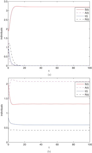
Second, we choose p=0.1, $\delta =0.1$, m=0.1, numerical simulation gives $R_0=2.4381$, $\tau =0$, then the alcohol-present equilibrium $E^{\ast }$ is globally asymptotically stable (Figure  2(b)).

Third, we choose p=0.9, $\delta =0.7$, m=0.9, numerical simulation gives $R_0=0.6898,\tau =3$, then the alcohol-free equilibrium $E_0$ is globally asymptotically stable (Figure 3(a)).

Figure 3. The densities of $S\left(t\right),A\left(t\right),I\left(t\right)$ and $R\left(t\right)$ change when $R_0<1,\tau =3\left(a\right)$ and $R_0>1,\tau =3\left(b\right)$.

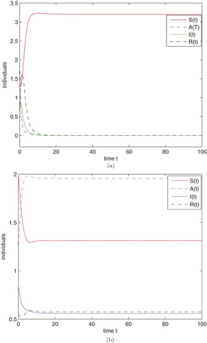
At last, we choose p=0.1, $\delta =0.1$, m=0.1, numerical simulation gives $R_0=2.4381$, $\tau =3$, then the alcohol-present equilibrium $E^{\ast }$ is globally asymptotically stable (Figure  3(b)).

6. Discussion

We have formulated a more realistic drinking model with two stages and time delay. We obtain the basic reproduction number $R_0$ of the model. For the model without time delay, the alcohol-free equilibrium is locally asymptotically stable if the basic reproduction number $R_0<1$. When $R_0>1$, there exists a unique alcohol-present equilibrium which is locally asymptotically stable under a certain condition. For the model with time delay, the stability of all the equilibria are obtained. Furthermore, regardless of the time delay length, using comparison theorem and iteration technique, we obtain that the alcohol-free equilibrium is globally asymptotically stable. Numerical simulations also confirm the theoretical results.

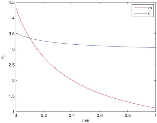
Direct calculation can show that $\mathrm{\partial }{R}_0/\mathrm{\partial }\beta >0$, $\mathrm{\partial }{R}_0/\mathrm{\partial }\gamma >0$, $\mathrm{\partial }{R}_0/\mathrm{\partial }m<0$, $\mathrm{\partial }{R}_0/\mathrm{\partial }\delta <0$, then decreasing contact rate and increasing the treat rate are helpful to reduce the alcohol abuse. By Figure 4, we can see that $R_0$ increases with the increase of β or γ, that means higher contact rate can increase the propagation of alcoholism. Figure 5 shows the relation among the basic reproduction number $R_0$, the treat coefficient δ and m. From Figure 5, we find that it is obvious that m works more effective than δ. Therefore, it is important to treat light problem alcoholics in order to control the propagation of alcoholism.

Figure 4. The relationship between the basic reproduction number $R_0$ and the parameters $\beta ,\gamma$.

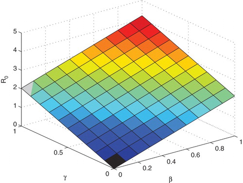
Figure 5. The relationship between the basic reproduction number $R_0$ and the parameters $m,\delta$.($\mathrm{\Lambda }=0.8,\mu =0.25,\beta =0.3,\gamma =0.15,\eta =0.4,p=0.1,\delta =0.1,m=0.1,\tau =3$).

It is easy to see the time delay can influence the dynamic behaviours of the system. From Equation (4(4) $R_0=\frac{\left[\beta \right(\mu +\delta )+p\gamma ]\mathrm{\Lambda }}{\mu (\mu +\delta )(\mu +m+p)}.$(4) ) we know that $R_0$ is independent of the time delay. However, the stability of equilibria in the model depends on the time delay. It is obvious that time delay can influence the stability of the alcohol-free equilibrium according to Theorems  4.3 and 4.4.

Disclosure statement

No potential conflict of interest was reported by the authors.

Additional information

Funding

This work is partially supported by the Nature Science Foundation of China (11461041, 11661050), the Nature Science Foundation of Gansu Province of China (148RJZA024) and the Development Program for HongLiu Distinguished Young Scholars in Lanzhou University of Technology.

References

- M.M. Glavas and J. Weinberg, Stress, alcohol consumption and the hypothalamicpituitary adrenal axis, in Nutrients, Stress and Medical Disorders, Humana Press, New York, 2006, pp. 165–183.
- J.K. Hale, Theory of Functional Differential Equations, Springer, New York, 1997.
- H.F. Huo and L.X. Feng, Global stability for an HIV/AIDS epidemic model with different latent stages and treatment, Appl. Math. Model. 37 (2013), pp. 1480–1489. doi: 10.1016/j.apm.2012.04.013
- H.F. Huo, S.H. Ma and X.Y. Meng, Modelling Alcoholism as a Contagious Disease: A Mathematical Model with Awareness Programs and Time Delay, Discret. Dyn. Nat Soc. 2015 Article ID 260195 (13 pages), 2015.
- H.F. Huo and X.M. Zhang, Complex dynamics in an alcoholism model with the impact of Twitter, Math. Biosci. 281 (2016), pp. 24–35. doi: 10.1016/j.mbs.2016.08.009
- M. Inoue, Association between alcohol consumption and colorectal cancer risk, Cur. Nutrition Rep, 2 (2013), pp. 71–73. doi: 10.1007/s13668-012-0033-z
- L.D. Johnston, P.M. OMalley and J.G. Bachman, National Survey Results on Drug use from the Monitoring the Future Study, 1975–1992, National Institute on Drug Abuse, Rockville, MD, 1993.
- S. Lee, E. Jung and C. Castillo-Chavez, Optimal control intervention strategies in low- and high-risk problem drinking populations, Socio-Econ. Plan. Sci. 44 (2010), pp. 258–265. doi: 10.1016/j.seps.2010.07.006
- P.M. O'Malley and L.D. Johnston, Epidemiology of alcohol and other drug use among American college students, J. Stud. Alcohol 63(14) (2002), pp. 23–39. doi: 10.15288/jsas.2002.s14.23
- J.L. Manthey, A.Y. Aidoob and K.Y. Ward, Campus drinking: an epidemiolodical model, J. Biol. Dyn. 2 (2008), pp. 346–356. doi: 10.1080/17513750801911169
- A. Mubayi, P.E. Greenwood, C. Castillo-Chavez, P.J. Gruenewald and D.M. Gorman, The impact of relative residence times on the distribution of heavy drinkers in highly distinct environments, Socio-Econ. Plan. Sci. 44(1) (2010), pp. 45–56. doi: 10.1016/j.seps.2009.02.002
- G. Mulone and B. Straughan, Modeling binge drinking, Int. J. Biomath. 5(1) (2012), pp. 1250005. (14 pages). doi: 10.1142/S1793524511001453
- S. Mushayabasa and C.P. Bhunu, Modelling the effects of heavy alcohol consumption on the transmission dynamics of gonorrhea, Nonlinear Dyn. 66 (2011), pp. 695–706. doi: 10.1007/s11071-011-9942-4
- National Institute on Alcohol Abuse and Alcoholism, Department of Health and Human Services, United States of America. Available at http://www.niaaa.nih.gov/alcohol-health, last accessed March 11, 2016.
- J. Rehm, The risk associated with alcohol use and alcoholism, Alcohol Res. Health 34 (2011), pp. 135–143.
- J. Ribes, R. Clèries, L. Esteban, V. Moreno, and F.X. Bosch, The influence of alcohol consumption and hepatitis B and Cinfections on the risk of liver cancer in Europe, J. Hepatol. 49(2) (2008), pp. 233–242. doi: 10.1016/j.jhep.2008.04.016
- O. Sharomi and A.B. Gumel, Curtailing smoking dynamics: a mathematical modeling approach, Appl. Math. Comput. 195 (2008), pp. 475–499. doi: 10.1016/j.amc.2007.05.012
- X.Y. Wang, K. Hattaf, H.F. Huo and H. Xiang, Stability analysis of a delayed social epidemics model with general contact rate and its optimal control, J. Indus. Manag. Optim. 12 (2016), pp. 1267–1285. doi: 10.3934/jimo.2016.12.1267
- H. Wechsler, J.E. Lee, T.F. Nelson and M.C. Kuo, Underage college students drinking behavior, access to alcohol, and the influence of deterrence policies, J. Amer. College Health 50(5) (2002), pp. 223–236. doi: 10.1080/07448480209595714
- H. Wechsler, J.E. Lee, M. Kuo and H. Lee, College binge drinking in the 1990s:a continuing problem.Results of the Harvard School of Public Health 1999 College Alcohol Study, J. Amer. College Health 48(5) (2000), pp. 199–210. doi: 10.1080/07448480009599305
- WHO, Global Status Report on Alcohol and Health 2014, WHO, Geneva, Switzerland, 2014.
- H. Xiang, L.X. Feng and H.F. Huo, Stability of the virus dynamics model with Beddington–DeAngelis functional response and delays, Appl. Math. Model. 37 (2013), pp. 5414–5423. doi: 10.1016/j.apm.2012.10.033
- H. Xiang, N.N. Song and H.F. Huo, Modelling effects of public health educational campaigns on drinking dynamics, J. Biol. Dyn. 10 (2016), pp. 164–178. doi: 10.1080/17513758.2015.1115562
- H. Xiang, Y.L. Tang and H.F. Huo, A viral model with intracellular delay and humoral immunity, Bull. Malays. Math. Sci. Soc. (2016) doi: 10.1007/s40840-016-0326-2.
- G. Zaman, Qualitative behavior of giving up smoking models, Bull. Malays. Math. Sci. Soc. 34 (2009), pp. 403–415.