Optimal control of a social epidemic model with media coverage

ABSTRACT

A new social epidemic model to depict alcoholism with media coverage is proposed in this paper. Some fundamental properties of the model including existence and positivity as well as boundedness of equilibria are investigated. Stability of all equilibria are studied. The existence of the optimal control pair and mathematical expressions of optimal control are obtained by Pontryagin's maximum principle. Numerical simulations are also performed to illustrate our results. Our results show that media coverage is an effective measure to quit drinking.

KEYWORDS:

• Alcoholism
• media coverage
• stability
• optimal control

1. Introduction

The mathematical modelling of topics involving alcoholism is becoming an important area [9, 15, 22]. There is a strong evidence that alcoholism is associated with many health problems and the global burden of disease [22]. Alcohol consumption has negative effects on all organs of the body. Approximately, worldwide 3.6% of cancers derive from chronic alcohol drinking, including those of the upper aerodigestive tract, the liver, the colorectum and the breast [9]. It has observed a significant indirect relationship between the degree of working memory decline induced by alcohol and adverse consequences of alcohol use [15]. There are many valid ways to quit drinking, such as gradually reducing the amount of alcohol or taking tablets and so on. A number of mathematical models for alcoholism has been established and analysed [19, 24, 26]. As early as 1953, Stratus and Bacon began to research classical problem of college students drinking [26]. Sanchez et al. [24] divided the people into three classes, namely susceptible, alcoholics, alcoholics undergoing treatment. They assumed that each of the three parts had the same death rate and took into account relapse, but they ignored the death rate due to heavy alcohol consumption. Mulone and Straughan [19] studied a model for binge drinking taking into account admitting and non-admitting drinkers. For the other mathematical models about drinking, smoking or epidemics, we refer to [3–5, 10, 11, 20, 25, 29–31] and the references cited therein.

Nowadays, media can play an important role in the spread and control of infectious disease. Media usually can cut down the opportunity and probability of contact transmission of disease. Liu et al. [17] constructed a new model to explain the mechanism for outbreaks of emerging infectious diseases due to the psychological effect of the reported numbers of infectious and hospitalized individuals. Samanta et al. [23] built a mathematical model to study the impact of awareness programs by media on the emergence of infectious diseases. Liu and Cui [16] set up a model to investigate the impact of media coverage and controlling of infectious disease in a given region. Ma et al. [18] introduced a dynamic alcohol consumption model with awareness programs and time delay and captured the effects of awareness programs and time delay in controlling the alcohol problems.

Different control strategies, such as education campaigns, resource allocation, vaccination and treatment, are used in many epidemic models [1, 2, 6, 13]. Zaman [32] considered two possible control variables in the form of education and treatment campaigns oriented to decrease smoking. Wang et al. [28] formulated an alcohol quitting model in which they consider the impact of distributed time delay between contact and infection process by characterizing dynamic nature of alcoholism behaviours, and they generalized the infection rate to the general case. Furthermore they considered two control strategies,that is education and treatment.

The structure of this paper is organized as follows. In Section 2, a more realistic alcoholism model with media coverage is constructed. Motivated by Wang et al. [27], we use saturation function (Holling type-II) to reflect the influence of media on the alcoholics. In Section 3, the basic reproduction number and existence of alcoholism equilibrium are derived. In Section 4, stability analysis of equilibria of model is investigated by using Lyapunov function and Routh–Hurwitz criterion. In Section 5, optimal control strategies by using the classical method of Pontryagin's maximum principle are discussed. In Section 6, some sensitivity analysis and numerical simulations are presented. Some conclusions and discussions are also given.

2. Model formulation

The total population is divided into three compartments in our model, susceptible individuals who do not drink or drink only moderately, denoted by $P\left(t\right)$; alcoholics who binge drink and affect the physical health seriously, denoted by $A\left(t\right)$, the quitting drinkers who permanently quit drinking, denoted by $Q\left(t\right)$. It is supposed that the cumulative density of susceptible individuals and quitting drinkers driven by media coverage at time t is $M\left(t\right)$. The growth rate of $M\left(t\right)$ is proportional to the number of mortalities induced by alcoholics. The total number of population at time t is given by (1) $N\left(t\right)=P\left(t\right)+A\left(t\right)+Q\left(t\right).$(1)

The population flow among those compartments is shown in Figure 1.

Figure 1. Transfer diagram for alcoholism model with media coverage.

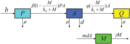
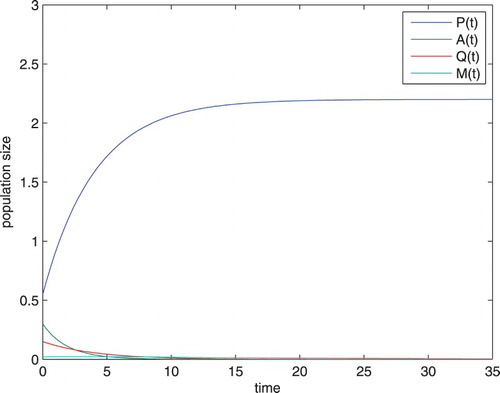
Figure 2. when $R_0<1$, the alcohol free equilibrium $E_0$ is globally asymptotically stable.

The mathematical representation of the model consists of a system of nonlinear differential equations with four state variables. The complete model is as follows: (2) $\begin{array}{rl}\frac{\mathrm{d}P}{\mathrm{d}t}& =b-\beta (1-\frac{M}{k_0}+M)PA-\mu P,\\ \frac{\mathrm{d}A}{\mathrm{d}t}& =\beta (1-\frac{M}{k_0}+M)PA-q\frac{M}{k_1+MA}-(\mu +d)A,\\ \frac{\mathrm{d}Q}{\mathrm{d}t}& =q\frac{M}{k_1+M}A-\mu Q,\\ \frac{\mathrm{d}M}{\mathrm{d}t}& =mdA-\gamma M,\end{array}$(2) where b is the recruitment rate of susceptible individuals who do not drink or drink only moderately, β is the transmission coefficient form the susceptible individuals to the alcoholics. Large numbers of media coverage causes less interaction between susceptible aware and alcoholic populations, a mathematical form of this assumption follows the Holling type-II functional form with half-saturating constant $k_0$ (see [27]). Similarly, we use the Holling type-II functional form with half-saturating constant $k_1$ to reflect the effect of media coverage on alcoholics. q is the rate coefficient of the individuals who permanently quit drinking, μ is the natural death rate of the population, d is the death rate due to heavy alcohol consumption, m is the implementation rate of media coverage, γ is the depletion rate of media coverage due to ineffectiveness, social problems and similar factors.

Lemma 2.1

If $P\left(0\right)>0,$ $A\left(0\right)>0,$ $Q\left(0\right)>0,$ $M\left(0\right)>0,$ the solutions $P\left(t\right),$ $A\left(t\right),$ $Q\left(t\right),$ $M\left(t\right)$ of Equation (2(2) $\begin{array}{rl}\frac{\mathrm{d}P}{\mathrm{d}t}& =b-\beta (1-\frac{M}{k_0}+M)PA-\mu P,\\ \frac{\mathrm{d}A}{\mathrm{d}t}& =\beta (1-\frac{M}{k_0}+M)PA-q\frac{M}{k_1+MA}-(\mu +d)A,\\ \frac{\mathrm{d}Q}{\mathrm{d}t}& =q\frac{M}{k_1+M}A-\mu Q,\\ \frac{\mathrm{d}M}{\mathrm{d}t}& =mdA-\gamma M,\end{array}$(2) ) are positive for all t>0.

Proof.

If the conclusion dose not satisfy, then at least one of $P\left(t\right)$, $A\left(t\right)$, $Q\left(t\right)$, $M\left(t\right)$ is not positive. Thus, we have one of the following four cases.

1. There exists a first time $t_1$ such that $P\left(t_1\right)=0,P^{\prime }\left(t_1\right)<0,A\left(t\right)>0,Q\left(t\right)>0,M\left(t\right)>0,0\le t\le t_1.$

2. There exists a first time $t_2$ such that $A\left(t_2\right)=0,A^{\prime }\left(t_2\right)<0,P\left(t\right)>0,Q\left(t\right)>0,M\left(t\right)>0,0\le t\le t_2.$

3. There exists a first time $t_3$ such that $Q\left(t_3\right)=0,Q^{\prime }\left(t_3\right)<0,P\left(t\right)>0,A\left(t\right)>0,M\left(t\right)>0,0\le t\le t_3.$

4. There exists a first time $t_4$ such that $M\left(t_4\right)=0,M^{\prime }\left(t_4\right)<0,P\left(t\right)>0,A\left(t\right)>0,Q\left(t\right)>0,0\le t\le t_4.$ In cases (1), we have $P^{\prime }\left(t_1\right)=b>0,$ which is contradiction to $P^{\prime }\left(t_1\right)<0$.

In cases (2), we have $A^{\prime }\left(t_2\right)=0,$ which is contradiction to $A^{\prime }\left(t_2\right)<0$.

In cases (3), we have $Q^{\prime }\left(t_3\right)=q\frac{M}{k_1+M}A>0,$ which is contradiction to $Q^{\prime }\left(t_3\right)<0$.

In cases (4), we have $M^{\prime }\left(t_4\right)=mdA>0,$ which is contradiction to $M^{\prime }\left(t_4\right)<0$.

Thus, the solutions $P\left(t\right)$, $A\left(t\right)$, $Q\left(t\right)$, $M\left(t\right)$ of Equation (2(2) $\begin{array}{rl}\frac{\mathrm{d}P}{\mathrm{d}t}& =b-\beta (1-\frac{M}{k_0}+M)PA-\mu P,\\ \frac{\mathrm{d}A}{\mathrm{d}t}& =\beta (1-\frac{M}{k_0}+M)PA-q\frac{M}{k_1+MA}-(\mu +d)A,\\ \frac{\mathrm{d}Q}{\mathrm{d}t}& =q\frac{M}{k_1+M}A-\mu Q,\\ \frac{\mathrm{d}M}{\mathrm{d}t}& =mdA-\gamma M,\end{array}$(2) ) are positive for all t>0.

Lemma 2.2

All feasible solutions $P\left(t\right),$ $A\left(t\right),$ $Q\left(t\right),$ $M\left(t\right)$ of Equation (2(2) $\begin{array}{rl}\frac{\mathrm{d}P}{\mathrm{d}t}& =b-\beta (1-\frac{M}{k_0}+M)PA-\mu P,\\ \frac{\mathrm{d}A}{\mathrm{d}t}& =\beta (1-\frac{M}{k_0}+M)PA-q\frac{M}{k_1+MA}-(\mu +d)A,\\ \frac{\mathrm{d}Q}{\mathrm{d}t}& =q\frac{M}{k_1+M}A-\mu Q,\\ \frac{\mathrm{d}M}{\mathrm{d}t}& =mdA-\gamma M,\end{array}$(2) ) are bounded by the region (3) $\mathrm{\Omega }=\left\{\right(P,A,Q,M)\in R_4^{+}:P+A+Q\le \frac{b}{\mu },0\le M\le \frac{mdb}{\mu \gamma }\}.$(3)

Proof.

Parameters of Equation (2(2) $\begin{array}{rl}\frac{\mathrm{d}P}{\mathrm{d}t}& =b-\beta (1-\frac{M}{k_0}+M)PA-\mu P,\\ \frac{\mathrm{d}A}{\mathrm{d}t}& =\beta (1-\frac{M}{k_0}+M)PA-q\frac{M}{k_1+MA}-(\mu +d)A,\\ \frac{\mathrm{d}Q}{\mathrm{d}t}& =q\frac{M}{k_1+M}A-\mu Q,\\ \frac{\mathrm{d}M}{\mathrm{d}t}& =mdA-\gamma M,\end{array}$(2) ) are assumed to be positive. Using the fact $N\left(t\right)=P\left(t\right)+A\left(t\right)+Q\left(t\right)$, the system (2(2) $\begin{array}{rl}\frac{\mathrm{d}P}{\mathrm{d}t}& =b-\beta (1-\frac{M}{k_0}+M)PA-\mu P,\\ \frac{\mathrm{d}A}{\mathrm{d}t}& =\beta (1-\frac{M}{k_0}+M)PA-q\frac{M}{k_1+MA}-(\mu +d)A,\\ \frac{\mathrm{d}Q}{\mathrm{d}t}& =q\frac{M}{k_1+M}A-\mu Q,\\ \frac{\mathrm{d}M}{\mathrm{d}t}& =mdA-\gamma M,\end{array}$(2) ) reduced to the following system: (4) $\begin{array}{rl}\frac{\mathrm{d}A}{\mathrm{d}t}& =\beta (1-\frac{M}{k_0}+M)(N-A-Q)A-(\mu +d)A-q\frac{M}{k_1}+MA,\\ \frac{\mathrm{d}Q}{\mathrm{d}t}& =q\frac{M}{k_1}+MA-\mu Q,\\ \frac{\mathrm{d}N}{\mathrm{d}t}& =b-\mu N-\mathrm{d}A,\\ \frac{\mathrm{d}M}{\mathrm{d}t}& =mdA-\gamma M.\end{array}$(4) From the third equation in (3(3) $\mathrm{\Omega }=\left\{\right(P,A,Q,M)\in R_4^{+}:P+A+Q\le \frac{b}{\mu },0\le M\le \frac{mdb}{\mu \gamma }\}.$(3) ) we can obtain (5) $\frac{\mathrm{d}N}{\mathrm{d}t}=b-\mu N-\mathrm{d}A\le b-\mu N.$(5) It follows that (6) $N\left(t\right)\le \frac{b}{\mu }+N\left(0\right){\mathrm{e}}^{-\mu t},$(6) where $N\left(0\right)$ is the initial value of total number of people. Thus, (7) $\underset{t\to \mathrm{\infty }}{lim}supN\left(t\right)\le \frac{b}{\mu },$(7) then (8) $P\left(t\right)+A\left(t\right)+Q\left(t\right)\le \frac{b}{\mu }.$(8) Form the fourth equation in (3(3) $\mathrm{\Omega }=\left\{\right(P,A,Q,M)\in R_4^{+}:P+A+Q\le \frac{b}{\mu },0\le M\le \frac{mdb}{\mu \gamma }\}.$(3) ), we have (9) $\frac{\mathrm{d}M}{\mathrm{d}t}=mdA-\gamma M\le m\frac{\mathrm{d}b}{\mu }-\gamma M,$(9) it follows that (10) $0\le M\left(t\right)\le \frac{mdb}{\mu \gamma }+M\left(0\right){\mathrm{e}}^{-\gamma t},$(10) where $M\left(0\right)$ represents the initial value of cumulative density media coverage. Thus, (11) $\underset{t\to \mathrm{\infty }}{lim}supM\left(t\right)\le \frac{mdb}{\mu \gamma }.$(11) Hence, for the analysis of model (2(2) $\begin{array}{rl}\frac{\mathrm{d}P}{\mathrm{d}t}& =b-\beta (1-\frac{M}{k_0}+M)PA-\mu P,\\ \frac{\mathrm{d}A}{\mathrm{d}t}& =\beta (1-\frac{M}{k_0}+M)PA-q\frac{M}{k_1+MA}-(\mu +d)A,\\ \frac{\mathrm{d}Q}{\mathrm{d}t}& =q\frac{M}{k_1+M}A-\mu Q,\\ \frac{\mathrm{d}M}{\mathrm{d}t}& =mdA-\gamma M,\end{array}$(2) ), we get the region which is given by the set: (12) $\mathrm{\Omega }=\left\{\right(P,A,Q,M)\in R_4^{+}:P+A+Q\le \frac{b}{\mu },0\le M\le \frac{mdb}{\mu \gamma }\},$(12) which is a positively invariant set for (2(2) $\begin{array}{rl}\frac{\mathrm{d}P}{\mathrm{d}t}& =b-\beta (1-\frac{M}{k_0}+M)PA-\mu P,\\ \frac{\mathrm{d}A}{\mathrm{d}t}& =\beta (1-\frac{M}{k_0}+M)PA-q\frac{M}{k_1+MA}-(\mu +d)A,\\ \frac{\mathrm{d}Q}{\mathrm{d}t}& =q\frac{M}{k_1+M}A-\mu Q,\\ \frac{\mathrm{d}M}{\mathrm{d}t}& =mdA-\gamma M,\end{array}$(2) ). So we only need to consider dynamics of system on the set Ω.

3. Basic reproduction number and alcohol free equilibrium

It is easy to know that system (2(2) $\begin{array}{rl}\frac{\mathrm{d}P}{\mathrm{d}t}& =b-\beta (1-\frac{M}{k_0}+M)PA-\mu P,\\ \frac{\mathrm{d}A}{\mathrm{d}t}& =\beta (1-\frac{M}{k_0}+M)PA-q\frac{M}{k_1+MA}-(\mu +d)A,\\ \frac{\mathrm{d}Q}{\mathrm{d}t}& =q\frac{M}{k_1+M}A-\mu Q,\\ \frac{\mathrm{d}M}{\mathrm{d}t}& =mdA-\gamma M,\end{array}$(2) ) always has an alcohol free equilibrium $E_0=(b/\mu ,0,0,0)$. In the following, the basic reproduction number of system (2(2) $\begin{array}{rl}\frac{\mathrm{d}P}{\mathrm{d}t}& =b-\beta (1-\frac{M}{k_0}+M)PA-\mu P,\\ \frac{\mathrm{d}A}{\mathrm{d}t}& =\beta (1-\frac{M}{k_0}+M)PA-q\frac{M}{k_1+MA}-(\mu +d)A,\\ \frac{\mathrm{d}Q}{\mathrm{d}t}& =q\frac{M}{k_1+M}A-\mu Q,\\ \frac{\mathrm{d}M}{\mathrm{d}t}& =mdA-\gamma M,\end{array}$(2) ) will be obtained by the next generation matrix method formulated in [7]. Let $x=(P,A,Q,M{)}^{\mathrm{T}}$, system (2(2) $\begin{array}{rl}\frac{\mathrm{d}P}{\mathrm{d}t}& =b-\beta (1-\frac{M}{k_0}+M)PA-\mu P,\\ \frac{\mathrm{d}A}{\mathrm{d}t}& =\beta (1-\frac{M}{k_0}+M)PA-q\frac{M}{k_1+MA}-(\mu +d)A,\\ \frac{\mathrm{d}Q}{\mathrm{d}t}& =q\frac{M}{k_1+M}A-\mu Q,\\ \frac{\mathrm{d}M}{\mathrm{d}t}& =mdA-\gamma M,\end{array}$(2) ) can be written as $\frac{\mathrm{d}x}{\mathrm{d}t}=\mathcal{F}\left(x\right)-\mathcal{V}\left(x\right),$ where $\begin{array}{rl}\mathcal{F}\left(x\right)& =\left(\begin{array}{c}\beta (1-\frac{M}{k_0}+M)\\ P\\ 0\\ 0\\ 0\end{array}\right),\\ \mathcal{V}\left(x\right)& =\left(\begin{array}{c}(\mu +d)A+q\frac{M}{k_1+M}A\\ \mu Q-q\frac{M}{k_1+M}A\\ \gamma M-mdA\\ \beta (1-\frac{M}{k_0+M})PA+\mu P-b\end{array}\right).\end{array}$ The Jacobian matrices of $\mathcal{F}\left(x\right)$ and $\mathcal{V}\left(x\right)$ at the alcohol free equilibrium $E_0$ are, respectively, $\begin{array}{rl}D\mathcal{F}\left(E_0\right)& =\left(\begin{array}{cc}{F}_{2\times 2}& 0\\ 0& 0\end{array}\right),\\ D\mathcal{V}\left(E_0\right)& =\left(\begin{array}{cccc}{V}_{2\times 2}& & 0& 0\\ -md& 0& \gamma & 0\\ \beta \frac{b}{\mu }& 0& 0& \mu \end{array}\right),\end{array}$ where $\begin{array}{rl}F& =\left(\begin{array}{cc}\beta \frac{b}{\mu }& 0\\ 0& 0\end{array}\right),\\ V& =\left(\begin{array}{cc}\mu +d& 0\\ 0& \mu \end{array}\right).\end{array}$ The basic reproduction number is $R_0=\rho \left(F{V}^{-1}\right)=\frac{b\beta }{\mu (\mu +d)}.$

By the Theorem 2 of [7], we have the following theorem.

Theorem 3.1

For system (2(2) $\begin{array}{rl}\frac{\mathrm{d}P}{\mathrm{d}t}& =b-\beta (1-\frac{M}{k_0}+M)PA-\mu P,\\ \frac{\mathrm{d}A}{\mathrm{d}t}& =\beta (1-\frac{M}{k_0}+M)PA-q\frac{M}{k_1+MA}-(\mu +d)A,\\ \frac{\mathrm{d}Q}{\mathrm{d}t}& =q\frac{M}{k_1+M}A-\mu Q,\\ \frac{\mathrm{d}M}{\mathrm{d}t}& =mdA-\gamma M,\end{array}$(2) ), the alcohol free equilibrium $E_0$ is locally asymptotically stable if $R_0<1$ and unstable for $R_0>1$.

$R_0$ is basic reproduction number of the model. It measures the average number of new alcoholics generated by a alcoholics in a population of susceptible drinkers.

Theorem 3.2

If $R_0<1,$ the alcohol free equilibrium $E_0$ is globally asymptotically stable.

Proof.

Constructing Lyapunov function as follows: (13) $V=P-P_0-P_0\ln \frac{P}{P_0}+A+Q.$(13) The derivative of $V$ along with (2(2) $\begin{array}{rl}\frac{\mathrm{d}P}{\mathrm{d}t}& =b-\beta (1-\frac{M}{k_0}+M)PA-\mu P,\\ \frac{\mathrm{d}A}{\mathrm{d}t}& =\beta (1-\frac{M}{k_0}+M)PA-q\frac{M}{k_1+MA}-(\mu +d)A,\\ \frac{\mathrm{d}Q}{\mathrm{d}t}& =q\frac{M}{k_1+M}A-\mu Q,\\ \frac{\mathrm{d}M}{\mathrm{d}t}& =mdA-\gamma M,\end{array}$(2) ) is given by (14) $\begin{array}{rl}{V}^{\prime }& =P^{\prime }-\frac{P_0}{P}{P}^{\prime }+A^{\prime }+Q^{\prime }\\ & =b-\beta (1-\frac{M}{k_0+M})PA-\mu P-\frac{P_0}{P}[b-\beta (1-\frac{M}{k_0+M})PA-\mu P]\\ & +\beta (1-\frac{M}{k_0+M})PA-q\frac{M}{k_1+M}A-(\mu +d)A+q\frac{M}{k_1+M}A-\mu Q\\ & =b-\mu P-\frac{P_0}{P}b+\beta (1-\frac{M}{k_0+M})P_{0}A+\mu P_0-(\mu +d)A-\mu Q\\ & =b-\mu P-\frac{b^2}{\mu P}+\frac{\beta b}{\mu }(1-\frac{M}{k_0+M})A+b-(\mu +d)A-\mu Q\\ & \le b(2-\frac{b}{\mu P}-\frac{\mu P}{b})+\frac{\beta b}{\mu }[1-\frac{(\mu +d)\mu }{\beta b}]A-\mu Q.\end{array}$(14)

Obviously, $2-b/\mu P-\mu P/b\le 0$, and if $R_0<1$, we can get that $1-(\mu +d)\mu /\beta b<0$, hence, we obtain $V^{\prime }\le 0$. Furthermore, $V^{\prime }=0$ holds if and only if $2-b/\mu P-\mu P/b=0$, A=0, Q=0. By LaSalle's invariance principle [14], we can derive that the alcohol free equilibrium $E_0$ is globally asymptotically stable. The proof is complete.

4. Existence and stability of alcohol present equilibrium

The alcohol present equilibrium $E^{\ast }=(P^{\ast },A^{\ast },Q^{\ast },M^{\ast })$ of system (2(2) $\begin{array}{rl}\frac{\mathrm{d}P}{\mathrm{d}t}& =b-\beta (1-\frac{M}{k_0}+M)PA-\mu P,\\ \frac{\mathrm{d}A}{\mathrm{d}t}& =\beta (1-\frac{M}{k_0}+M)PA-q\frac{M}{k_1+MA}-(\mu +d)A,\\ \frac{\mathrm{d}Q}{\mathrm{d}t}& =q\frac{M}{k_1+M}A-\mu Q,\\ \frac{\mathrm{d}M}{\mathrm{d}t}& =mdA-\gamma M,\end{array}$(2) ) is determined by equations (15) $\begin{array}{rl}b-\beta (1-\frac{M}{k_0+M})PA-\mu P& =0,\\ \beta (1-\frac{M}{k_0+M})PA-(\mu +d)A-q\frac{M}{k_1+M}A& =0,\\ q\frac{M}{k_1+M}A-\mu Q& =0,\\ mdA-\gamma M& =0.\end{array}$(15) From the fourth equation in (15(15) $\begin{array}{rl}b-\beta (1-\frac{M}{k_0+M})PA-\mu P& =0,\\ \beta (1-\frac{M}{k_0+M})PA-(\mu +d)A-q\frac{M}{k_1+M}A& =0,\\ q\frac{M}{k_1+M}A-\mu Q& =0,\\ mdA-\gamma M& =0.\end{array}$(15) ), we have (16) $M=\frac{mdA}{\gamma }.$(16) From the third equation in (15(15) $\begin{array}{rl}b-\beta (1-\frac{M}{k_0+M})PA-\mu P& =0,\\ \beta (1-\frac{M}{k_0+M})PA-(\mu +d)A-q\frac{M}{k_1+M}A& =0,\\ q\frac{M}{k_1+M}A-\mu Q& =0,\\ mdA-\gamma M& =0.\end{array}$(15) ), and together with (16(16) $M=\frac{mdA}{\gamma }.$(16) ), we can get (17) $Q=\frac{q\frac{M}{k_1+M}A}{\mu }=\frac{qmd{A}^2}{\mu (k_1\gamma +mdA)}.$(17) From the second equation of (15(15) $\begin{array}{rl}b-\beta (1-\frac{M}{k_0+M})PA-\mu P& =0,\\ \beta (1-\frac{M}{k_0+M})PA-(\mu +d)A-q\frac{M}{k_1+M}A& =0,\\ q\frac{M}{k_1+M}A-\mu Q& =0,\\ mdA-\gamma M& =0.\end{array}$(15) ), and together with (16(16) $M=\frac{mdA}{\gamma }.$(16) ), we can get (18) $P=\frac{(\mu +d)+q\frac{M}{k_1+M}}{\beta (1-\frac{M}{k_0+M})}=\frac{\left[\right(\gamma k_1+mdA\left)\right(\mu +d)+qmdA](\gamma k_0+mdA)}{\gamma \beta k_0(\gamma k_1+mdA)}.$(18) Then substituting Equations (16(16) $M=\frac{mdA}{\gamma }.$(16) ) and (18(18) $P=\frac{(\mu +d)+q\frac{M}{k_1+M}}{\beta (1-\frac{M}{k_0+M})}=\frac{\left[\right(\gamma k_1+mdA\left)\right(\mu +d)+qmdA](\gamma k_0+mdA)}{\gamma \beta k_0(\gamma k_1+mdA)}.$(18) ) into the first equation in (15(15) $\begin{array}{rl}b-\beta (1-\frac{M}{k_0+M})PA-\mu P& =0,\\ \beta (1-\frac{M}{k_0+M})PA-(\mu +d)A-q\frac{M}{k_1+M}A& =0,\\ q\frac{M}{k_1+M}A-\mu Q& =0,\\ mdA-\gamma M& =0.\end{array}$(15) ), we have a quadratic equation of $A$ as follows: (19) $a_1(A{)}^2+a_2\left(A\right)+a_3=0,$(19) where (20) $\begin{array}{rl}{a}_1& =\gamma \beta k_{0}md(\mu +d)+\gamma \beta k_{0}qmd+\mu m^2{d}^2(\mu +d)+\mu q{m}^2{d}^2\\ a_2& =\gamma \beta k_0\gamma k_1(\mu +d)+\mu md(\mu +d)(\gamma k_1+\gamma k_0)+\mu q\gamma k_{0}md-b\gamma \beta k_{0}md\\ a_3& =k_0{k}_1{\gamma }^2\left[\mu \right(\mu +d)-b\beta ]=k_0{k}_1{\gamma }^2\mu (\mu +d)[1-R_0].\end{array}$(20)

It is easy to see that $a_1$ is always positive and $a_3$ is always negative if $R_0>1$. Hence, Equation (19(19) $a_1(A{)}^2+a_2\left(A\right)+a_3=0,$(19) ) has an unique positive root $A^{\ast }$.

Through the above conclusion, the following result holds.

Theorem 4.1

When $R_0>1,$ system (2(2) $\begin{array}{rl}\frac{\mathrm{d}P}{\mathrm{d}t}& =b-\beta (1-\frac{M}{k_0}+M)PA-\mu P,\\ \frac{\mathrm{d}A}{\mathrm{d}t}& =\beta (1-\frac{M}{k_0}+M)PA-q\frac{M}{k_1+MA}-(\mu +d)A,\\ \frac{\mathrm{d}Q}{\mathrm{d}t}& =q\frac{M}{k_1+M}A-\mu Q,\\ \frac{\mathrm{d}M}{\mathrm{d}t}& =mdA-\gamma M,\end{array}$(2) ) has an unique positive alcohol present equilibrium $E^{\ast }=(P^{\ast },A^{\ast },Q^{\ast },M^{\ast })$.

Next we consider the stability of the alcohol present equilibrium.

Theorem 4.2

For the system (2(2) $\begin{array}{rl}\frac{\mathrm{d}P}{\mathrm{d}t}& =b-\beta (1-\frac{M}{k_0}+M)PA-\mu P,\\ \frac{\mathrm{d}A}{\mathrm{d}t}& =\beta (1-\frac{M}{k_0}+M)PA-q\frac{M}{k_1+MA}-(\mu +d)A,\\ \frac{\mathrm{d}Q}{\mathrm{d}t}& =q\frac{M}{k_1+M}A-\mu Q,\\ \frac{\mathrm{d}M}{\mathrm{d}t}& =mdA-\gamma M,\end{array}$(2) ), the alcohol present equilibrium $E^{\ast }=(P^{\ast },A^{\ast },Q^{\ast },M^{\ast })$ is locally asymptotically stable if $R_0>1$.

Proof.

For the alcohol present equilibrium $E^{\ast }$, the matrix at $E^{\ast }$ can be written as (21) $J\left(E^{\ast }\right)=J^{\ast }=\left(\begin{array}{cccc}{J}_{11}^{\ast }& J_{12}^{\ast }& 0& J_{14}^{\ast }\\ J_{21}^{\ast }& J_{22}^{\ast }& 0& J_{24}^{\ast }\\ 0& J_{32}^{\ast }& J_{33}^{\ast }& J_{34}^{\ast }\\ 0& J_{42}^{\ast }& J_{44}^{\ast }\end{array}\right),$(21) where (22) $\begin{array}{rl}{J^{\ast }}_{11}& =-\beta \frac{k_0}{k_0+M^{\ast }}{A}^{\ast }-\mu ,{J^{\ast }}_{12}=-\beta \frac{k_0}{k_0+M^{\ast }}{P}^{\ast },{J^{\ast }}_{14}=\beta \frac{k_0}{{(k_0+M^{\ast })}^2}{P}^{\ast }{A}^{\ast },\\ {J^{\ast }}_{21}& =\beta \frac{k_0}{k_0+M^{\ast }}{A}^{\ast },{J^{\ast }}_{22}=\beta \frac{k_0}{k_0+M^{\ast }}{P}^{\ast }-(\mu +d)-q\frac{M^{\ast }}{k_1+M^{\ast }},\\ {J^{\ast }}_{24}& =-\beta \frac{k_0}{{(k_0+M^{\ast })}^2}{P}^{\ast }{A}^{\ast }-\frac{k_1}{{(k_1+M^{\ast })}^2}q{A}^{\ast },\\ {J^{\ast }}_{32}& =q\frac{M^{\ast }}{k_1+M^{\ast }},{J^{\ast }}_{33}=-\mu ,{J^{\ast }}_{34}=\frac{k_1}{{(k_1+M^{\ast })}^2}q{A}^{\ast },\\ {J^{\ast }}_{42}& =md,{J^{\ast }}_{44}=-\gamma .\end{array}$(22) So the characteristic equation at the alcohol present equilibrium $E^{\ast }$ is (23) ${\lambda }^4+d_1{\lambda }^3+d_2{\lambda }^2+d_3\lambda +d_4=0,$(23) where (24) $\begin{array}{rl}{d}_1& =-J_{11}^{\ast }-{J^{\ast }}_{22}-{J^{\ast }}_{33}-{J^{\ast }}_{44},\\ d_2& ={J^{\ast }}_{22}{J^{\ast }}_{44}-{J^{\ast }}_{24}{J^{\ast }}_{42}+{J^{\ast }}_{11}{J^{\ast }}_{22}+{J^{\ast }}_{11}{J^{\ast }}_{44}+{J^{\ast }}_{33}{J^{\ast }}_{22}+{J^{\ast }}_{33}{J^{\ast }}_{44}\\ & +{J^{\ast }}_{11}{J^{\ast }}_{33}-{J^{\ast }}_{21}{J^{\ast }}_{12},\\ d_3& =-{J^{\ast }}_{11}{J^{\ast }}_{22}{J^{\ast }}_{44}+{J^{\ast }}_{11}{J^{\ast }}_{24}{J^{\ast }}_{42}-{J^{\ast }}_{33}{J^{\ast }}_{22}{J^{\ast }}_{44}+{J^{\ast }}_{33}{J^{\ast }}_{24}{J^{\ast }}_{42}\\ & +{J^{\ast }}_{21}{J^{\ast }}_{12}{J^{\ast }}_{44}-{J^{\ast }}_{21}{J^{\ast }}_{14}{J^{\ast }}_{42}+{J^{\ast }}_{33}{J^{\ast }}_{21}{J^{\ast }}_{12}-{J^{\ast }}_{11}{J^{\ast }}_{22}{J^{\ast }}_{33}-{J^{\ast }}_{11}{J^{\ast }}_{33}{J^{\ast }}_{44},\\ d_4& ={J^{\ast }}_{11}{J^{\ast }}_{22}{J^{\ast }}_{33}{J^{\ast }}_{44}-{J^{\ast }}_{11}{J^{\ast }}_{33}{J^{\ast }}_{24}{J^{\ast }}_{42}-{J^{\ast }}_{21}{J^{\ast }}_{12}{J^{\ast }}_{33}{J^{\ast }}_{44}+{J^{\ast }}_{33}{J^{\ast }}_{21}{J^{\ast }}_{14}{J^{\ast }}_{42}.\end{array}$(24)

If $R_0>1$, it's obvious that ${J^{\ast }}_{ii}$ $(i=1,2,3,4,)$, ${J^{\ast }}_{12}$, ${J^{\ast }}_{24}$ are all negative and ${J^{\ast }}_{14}$, ${J^{\ast }}_{21}$, ${J^{\ast }}_{32}$, ${J^{\ast }}_{34}$, ${J^{\ast }}_{42}$ are all positive. Here, we only calculate $d_2>0$, (25) ${J^{\ast }}_{ii}{J^{\ast }}_{jj}(i=1,2,3,4,j=i+1,i+2,\dots 4)>0,{J^{\ast }}_{24}{J^{\ast }}_{42}>0,{J^{\ast }}_{21}{J^{\ast }}_{12}>0.$(25) Similarly, we can easily get the coefficients $d_i\left(i=1,3,4,\right)$ all are positive. According to the Routh–Hurwitz criterion [12], we can get that the eigenvalues of the above characteristic equation have negative real parts under the conditions (26) $\begin{array}{r}{d}_1{d}_2-d_3>0,\\ d_1{d}_2{d}_3-{d_3}^2-{d_1}^2{d}_4>0.\end{array}$(26) This shows that the alcohol present equilibrium $E^{\ast }$ is locally asymptotically stable if $R_0>1$.

Conjecture

If $R_0>1$, the alcohol present equilibrium $E^{\ast }$ is globally asymptotically stable.

Remark

It's difficult to demonstrate the global stability, we only present simulation. How to prove the global stability of alcohol present equilibrium $E^{\ast }$ have still to be resolved.

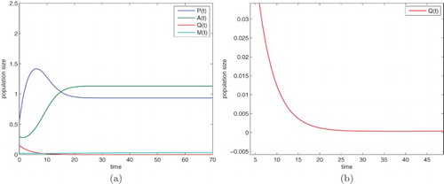
Figure 3. When $R_0>1$, the alcohol present equilibrium $E^{\ast }$ is globally asymptotically stable.

5. Optimal control problem

5.1. The existence of optimal control

In this section, in order to achieve the goal of minimized alcoholics, we reconsider the model (2(2) $\begin{array}{rl}\frac{\mathrm{d}P}{\mathrm{d}t}& =b-\beta (1-\frac{M}{k_0}+M)PA-\mu P,\\ \frac{\mathrm{d}A}{\mathrm{d}t}& =\beta (1-\frac{M}{k_0}+M)PA-q\frac{M}{k_1+MA}-(\mu +d)A,\\ \frac{\mathrm{d}Q}{\mathrm{d}t}& =q\frac{M}{k_1+M}A-\mu Q,\\ \frac{\mathrm{d}M}{\mathrm{d}t}& =mdA-\gamma M,\end{array}$(2) ) and formulate an optimal control problem (28(28) $\begin{array}{rl}\frac{\mathrm{d}P}{\mathrm{d}t}& =b-(1-u_1(t\left)\right)\beta (1-\frac{M}{k_0+M})PA-\mu P,\\ \frac{\mathrm{d}A}{\mathrm{d}t}& =(1-u_1(t\left)\right)\beta (1-\frac{M}{k_0+M})PA-q\frac{M}{k_1+M}A-(\mu +d)A-u_2\left(t\right)A,\\ \frac{\mathrm{d}Q}{\mathrm{d}t}& =q\frac{M}{k_1+M}A+u_2\left(t\right)A-\mu Q,\\ \frac{\mathrm{d}M}{\mathrm{d}t}& =mdA-\gamma M,\end{array}$(28) ) to reduce the numbers of alcoholics. Hence, we use two control variables $u_1\left(t\right)$ and $u_2\left(t\right)$ to reduce the number of alcoholics. The control $u_1\left(t\right)$ represents efforts intended to prevent the susceptible from contacting with the alcoholics, for example, the media coverage and educational programs are included. The control $u_2\left(t\right)$ represents the effort to encourage alcoholics to quit through proper treatment, such as taking pills or seeking other medical help. However, it is advisable to balance between the costs and the alcohol effects. In view of this, the optimal control problems to minimize the objective functional is given by (27) $J(u_1,u_2)={\int }_0^{t_f}\left[A\right(t)+\frac{1}{2}{b}_1{u}_1{\left(t\right)}^2+\frac{1}{2}{b}_2{u}_2{\left(t\right)}^2]\mathrm{d}t,$(27) subjects to (28) $\begin{array}{rl}\frac{\mathrm{d}P}{\mathrm{d}t}& =b-(1-u_1(t\left)\right)\beta (1-\frac{M}{k_0+M})PA-\mu P,\\ \frac{\mathrm{d}A}{\mathrm{d}t}& =(1-u_1(t\left)\right)\beta (1-\frac{M}{k_0+M})PA-q\frac{M}{k_1+M}A-(\mu +d)A-u_2\left(t\right)A,\\ \frac{\mathrm{d}Q}{\mathrm{d}t}& =q\frac{M}{k_1+M}A+u_2\left(t\right)A-\mu Q,\\ \frac{\mathrm{d}M}{\mathrm{d}t}& =mdA-\gamma M,\end{array}$(28) with initial conditions (29) $P\left(0\right)=P_0,A\left(0\right)=A_0,Q\left(0\right)=Q_0,M\left(0\right)=M_0.$(29) Here, $U=\left\{\right(u_1,u_2\left)|u_i\right(t)$ is measurable and $0\le u_i\left(t\right)\le 1$, for all $t\in [0,t_f]\}$, where $t_f$ is the final time, the constant $b_i\ge 0,i=1,2$ are relative weight coefficients that balance the cost and the number of alcoholics. The optimal control problem (28(28) $\begin{array}{rl}\frac{\mathrm{d}P}{\mathrm{d}t}& =b-(1-u_1(t\left)\right)\beta (1-\frac{M}{k_0+M})PA-\mu P,\\ \frac{\mathrm{d}A}{\mathrm{d}t}& =(1-u_1(t\left)\right)\beta (1-\frac{M}{k_0+M})PA-q\frac{M}{k_1+M}A-(\mu +d)A-u_2\left(t\right)A,\\ \frac{\mathrm{d}Q}{\mathrm{d}t}& =q\frac{M}{k_1+M}A+u_2\left(t\right)A-\mu Q,\\ \frac{\mathrm{d}M}{\mathrm{d}t}& =mdA-\gamma M,\end{array}$(28) )

Next, we will study andanalyse the existence of the optimal control. To determine existence of optimal control, we use the result of Fleming and Rishel [8].

Theorem 5.1

There exists an optimal control $u^{\ast }$ such that (30) $J({u_1}^{\ast },{u_2}^{\ast })=\min J(u_1,u_2),u_1\left(t\right),u_2\left(t\right)\in U.$(30) subjects to the control system (28(28) $\begin{array}{rl}\frac{\mathrm{d}P}{\mathrm{d}t}& =b-(1-u_1(t\left)\right)\beta (1-\frac{M}{k_0+M})PA-\mu P,\\ \frac{\mathrm{d}A}{\mathrm{d}t}& =(1-u_1(t\left)\right)\beta (1-\frac{M}{k_0+M})PA-q\frac{M}{k_1+M}A-(\mu +d)A-u_2\left(t\right)A,\\ \frac{\mathrm{d}Q}{\mathrm{d}t}& =q\frac{M}{k_1+M}A+u_2\left(t\right)A-\mu Q,\\ \frac{\mathrm{d}M}{\mathrm{d}t}& =mdA-\gamma M,\end{array}$(28) ) with initial conditions (29(29) $P\left(0\right)=P_0,A\left(0\right)=A_0,Q\left(0\right)=Q_0,M\left(0\right)=M_0.$(29) ).

Proof.

To prove the existence of an optimal control, the following conditions must be satisfied.

1. The controls and corresponding state variables are non-negative values.

2. The control set $U$ is convex and closed.

3. The right-hand side of the state system is bounded by a linear function in the state and control variables.

4. The integrand of the objective functional is concave on $U$.

5. There exist constants $c_1,c_2>0$ and $\alpha >1$ such that the integrant $L(t,u_1,u_2)\stackrel{\mathrm{\Delta }}{=}=A\left(t\right)+\frac{1}{2}{b}_1{u}_1(t{)}^2+\frac{1}{2}{b}_2{u}_2(t{)}^2$ of the objective functional satisfies (31) $L(t,u_1,u_2)\ge c_1(u_1(t{)}^2+u_2(t{)}^2{)}^{\alpha /2}-c_2.$(31) conditions 1, 2 and 4 are obvious satisfied. As for condition 3, we have already proved that four state variable are bounded, therefore, (32) $\frac{\mathrm{d}P}{\mathrm{d}t}\le b,\frac{\mathrm{d}A}{\mathrm{d}t}\le (1-u_1(t\left)\right)\beta PA,\frac{\mathrm{d}Q}{\mathrm{d}t}\le qA,\frac{\mathrm{d}M}{\mathrm{d}t}\le mdA.$(32) The last condition, we can easily see that there exist $c_1=min\{b_1/2,b_2/2\}$, and for all $c_2\in R^{+}$, $\alpha =2$ satisfies the equation $L(t,u_1,u_2)\ge c_1(u_1(t{)}^2+u_2(t{)}^2{)}^{\alpha /2}-c_2$, which completes the existence of an optimal control.

5.2. The characterization of the optimal control

Since the existence of the optimal control is established. The optimal control are obtained from the necessary conditions which come from the Pontryagin's Maximum Principle in [21]. To solve control problem actually, we should define Hamiltonian for the optimal control problems as follows: (33) $\begin{array}{rl}& H(P,A,Q,M,u_1,u_2,{\lambda }_1,{\lambda }_2,{\lambda }_3,{\lambda }_4)\\ & =A\left(t\right)+\frac{1}{2}{b}_1{u}_1(t{)}^2+\frac{1}{2}{b}_2{u}_2(t{)}^2\\ & +{\lambda }_1[b-(1-u_1\left(t\right))\beta (1-\frac{M}{k_0+M})PA-\mu P]\\ & +{\lambda }_2\left[\right(1-u_1\left(t\right))\beta (1-\frac{M}{k_0+M})PA-q\frac{M}{k_1+M}A-(\mu +d)A-u_2(t\left)A\right]\\ & +{\lambda }_3(q\frac{M}{k_1+M}A+u_2(t)A-\mu Q)+{\lambda }_4(mdA-\gamma M)\\ & -{\omega }_{11}{u}_1\left(t\right)-{\omega }_{12}(1-u_1(t\left)\right)-{\omega }_{21}{u}_2\left(t\right)-{\omega }_{22}(1-u_2(t\left)\right),\end{array}$(33) where ${\omega }_{11}\left(t\right)\ge 0$, ${\omega }_{12}\left(t\right)\ge 0$, are the penalty multipliers satisfying ${\omega }_{11}\left(t\right)u_1\left(t\right)={\omega }_{12}\left(t\right)(1-u_1(t\left)\right)=0,{\omega }_{21}\left(t\right)u_2\left(t\right)={\omega }_{22}\left(t\right)(1-u_2(t\left)\right)=0.$ at optimal control ${u_1}^{\ast }$ and ${u_2}^{\ast }$.

By applying Pontryagin's Maximum Principle we obtain the following theorem.

Theorem 5.2

There exist optimal control pairs $({u_1}^{\ast },{u_2}^{\ast })$ and state variable of $P\left(t\right),$ $A\left(t\right),$ $Q\left(t\right),$ $M\left(t\right)$ that minimize the objective functional $J(u_1,u_2)$ over U. Given these optimal controls, there exist adjoint variable ${\lambda }_1,{\lambda }_2,{\lambda }_3,{\lambda }_4,$ satisfying the equations (34) $\begin{array}{rl}{\lambda }_1^{\prime }& ={\lambda }_1(1-u_1(t\left)\right)\beta (1-\frac{M}{k_0+M})A+{\lambda }_1\mu -{\lambda }_2(1-u_1(t\left)\right)\beta (1-\frac{M}{k_0+M})A,\\ {\lambda }_2^{\prime }& =-1+{\lambda }_1(1-u_1(t\left)\right)\beta (1-\frac{M}{k_0+M})P-{\lambda }_2(1-u_1(t\left)\right)\beta (1-\frac{M}{k_0+M})P\\ & +{\lambda }_{2}q\frac{M}{k_1+M}+{\lambda }_2(\mu +d)-{\lambda }_{3}q\frac{M}{k_1+M}-{\lambda }_{4}md+{\lambda }_2{u}_2\left(t\right)-{\lambda }_3{u}_2\left(t\right),\\ {\lambda }_3^{\prime }& ={\lambda }_3\mu ,\\ {\lambda }_4^{\prime }& =-{\lambda }_1(1-u_1(t\left)\right)\beta \frac{k_0}{{(k_0+M)}^2}PA+{\lambda }_2(1-u_1(t\left)\right)\beta \frac{k_0}{{(k_0+M)}^2}PA\\ & +{\lambda }_{2}q\frac{k_1}{{(k_1+M)}^2}A-{\lambda }_{3}q\frac{k_1}{{(k_1+M)}^2}A+{\lambda }_4\gamma .\end{array}$(34) with the terminal conditions (35) ${\lambda }_i\left(t_f\right)=0,i=1,2,3,4.$(35) The optimal controls can be obtained from the following equations: (36) (n34) $\begin{array}{rl}{u_1}^{\ast }\left(t\right)& =min\left\{1,max\left\{0,\frac{1}{b_1}\left[\right({\lambda }_2-{\lambda }_1\left)\beta \right(1-\frac{M}{k_0+M}\left)PA\right]\right\}\right\},\\ {u_2}^{\ast }\left(t\right)& =min\left\{1,max\left\{0,\frac{({\lambda }_2-{\lambda }_3)A}{b_2}\right\}\right\}.\end{array}$(36) (n34)

Proof.

By differentiating the Hamiltonian, we obtain the adjoint system: (37) $\begin{array}{rl}{\lambda }_1^{\prime }& =-\frac{\mathrm{\partial }H}{\mathrm{\partial }P},{\lambda }_1\left(t_f\right)=0,{\lambda }_2^{\prime }=-\frac{\mathrm{\partial }H}{\mathrm{\partial }A},{\lambda }_2\left(t_f\right)=0.\\ {\lambda }_3^{\prime }& =-\frac{\mathrm{\partial }H}{\mathrm{\partial }Q},{\lambda }_3\left(t_f\right)=0,{\lambda }_4^{\prime }=-\frac{\mathrm{\partial }H}{\mathrm{\partial }M},{\lambda }_4\left(t_f\right)=0.\end{array}$(37) Therefore, the adjoint variable ${\lambda }_1,{\lambda }_2,{\lambda }_3,{\lambda }_4$ satisfy Equation (34(34) $\begin{array}{rl}{\lambda }_1^{\prime }& ={\lambda }_1(1-u_1(t\left)\right)\beta (1-\frac{M}{k_0+M})A+{\lambda }_1\mu -{\lambda }_2(1-u_1(t\left)\right)\beta (1-\frac{M}{k_0+M})A,\\ {\lambda }_2^{\prime }& =-1+{\lambda }_1(1-u_1(t\left)\right)\beta (1-\frac{M}{k_0+M})P-{\lambda }_2(1-u_1(t\left)\right)\beta (1-\frac{M}{k_0+M})P\\ & +{\lambda }_{2}q\frac{M}{k_1+M}+{\lambda }_2(\mu +d)-{\lambda }_{3}q\frac{M}{k_1+M}-{\lambda }_{4}md+{\lambda }_2{u}_2\left(t\right)-{\lambda }_3{u}_2\left(t\right),\\ {\lambda }_3^{\prime }& ={\lambda }_3\mu ,\\ {\lambda }_4^{\prime }& =-{\lambda }_1(1-u_1(t\left)\right)\beta \frac{k_0}{{(k_0+M)}^2}PA+{\lambda }_2(1-u_1(t\left)\right)\beta \frac{k_0}{{(k_0+M)}^2}PA\\ & +{\lambda }_{2}q\frac{k_1}{{(k_1+M)}^2}A-{\lambda }_{3}q\frac{k_1}{{(k_1+M)}^2}A+{\lambda }_4\gamma .\end{array}$(34) ). By differentiating the Hamiltonian with respect to the controls, we have the following optimality conditions: (38) $\begin{array}{rl}\frac{\mathrm{\partial }H}{\mathrm{\partial }{u}_1}=b_1{u}_1\left(t\right)+{\lambda }_1\beta (1-\frac{M}{k_0+M})PA-{\lambda }_2\beta (1-\frac{M}{k_0+M})PA-{\omega }_{11}+{\omega }_{12}& =0,\\ \frac{\mathrm{\partial }H}{\mathrm{\partial }{u}_2}=b_2{u}_2\left(t\right)-{\lambda }_{2}A+{\lambda }_{3}A-{\omega }_{21}+{\omega }_{22}& =0.\end{array}$(38)

To determined an explicit expression for the optimal control without ${\omega }_{11}$, ${\omega }_{12}$. We consider the following three cases.

1. For $\{t|0<{u_1}^{\ast }(t)<1\}$, we have ${\omega }_{11}\left(t\right)={\omega }_{12}\left(t\right)=0$. Hence the optimal control is (39) ${u_1}^{\ast }\left(t\right)=\frac{1}{b_1}\left[\right({\lambda }_2-{\lambda }_1\left)\beta (1-\frac{M}{k_0+M})PA\right].$(39)

2. For $\left\{t|{u_1}^{\ast }\right(t)=1\}$, we have ${\omega }_{11}\left(t\right)=0$. Hence (40) $1={u_1}^{\ast }\left(t\right)=\frac{1}{b_1}\left[\right({\lambda }_2-{\lambda }_1)\beta (1-\frac{M}{k_0+M})PA-{\omega }_{12}].$(40) Therefore, ${\omega }_{12}\left(t\right)\ge 0$ implies that (41) $\frac{1}{b_1}\left[\right({\lambda }_2-{\lambda }_1)\beta (1-\frac{M}{k_0+M})PA\ge 1.$(41)

3. For $\left\{t|{u_1}^{\ast }\right(t)=0\}$, we have ${\omega }_{12}\left(t\right)=0$. Hence, (42) $0={u_1}^{\ast }\left(t\right)=\frac{1}{b_1}\left[\right({\lambda }_2-{\lambda }_1)\beta (1-\frac{M}{k_0+M})PA+{\omega }_{11}].$(42) This implies that (43) $\frac{1}{b_1}({\lambda }_2-{\lambda }_1)\beta (1-\frac{M}{k_0+M})PA\le 0\mathrm{since}{\omega }_{11}\left(t\right)\ge 0.$(43) Combining these three cases, the optimal control is characterized as (44) ${u_1}^{\ast }\left(t\right)=min\left\{1,max\left\{0,\frac{1}{b_1}\left[({\lambda }_2-{\lambda }_1)\beta (1-\frac{M}{k_0+M})PA\right]\right\}\right\}.$(44) Similar to control variable ${u_1}^{\ast }\left(t\right)$, we get (45) ${u_2}^{\ast }\left(t\right)=min\left\{1,max\left\{0,\frac{({\lambda }_2-{\lambda }_3)A}{b_2}\right\}\right\}.$(45) This completes the proof.

6. Numerical simulations and discussions

In order to demonstrate the analytic results we have obtained, numerical experiments are carried out using Matlab. We choose a set of values of parameters in Table 1. We assume that the initial condition of (2(2) $\begin{array}{rl}\frac{\mathrm{d}P}{\mathrm{d}t}& =b-\beta (1-\frac{M}{k_0}+M)PA-\mu P,\\ \frac{\mathrm{d}A}{\mathrm{d}t}& =\beta (1-\frac{M}{k_0}+M)PA-q\frac{M}{k_1+MA}-(\mu +d)A,\\ \frac{\mathrm{d}Q}{\mathrm{d}t}& =q\frac{M}{k_1+M}A-\mu Q,\\ \frac{\mathrm{d}M}{\mathrm{d}t}& =mdA-\gamma M,\end{array}$(2) ) is $P\left(t\right)=0.55,A\left(t\right)=0.3,Q\left(t\right)=0.15,M\left(t\right)=0.02$. For the above set of parameter values, we obtain an unique positive alcohol present equilibrium $E^{\ast }=(1.8346,0.1645,0.00008113,0.0493)$.

Table 1. The parameters description of the alcoholism model.

$b$	Constant recruitment rate.	$0.55{\mathrm{year}}^{-1}$	estimated
$\mu$	Nature death rate.	$0.25{\mathrm{year}}^{-1}$	[19]
$\beta$	Transmission coefficient.	$0.03{\mathrm{year}}^{-1}$	[19]
$k_0$	Half-saturating constant.	$100{\mathrm{year}}^{-1}$	[18]
$k_1$	Half-saturating constant.	$80{\mathrm{year}}^{-1}$	estimated
$d$	Death rate due to heavy alcoholism.	$0.3{\mathrm{year}}^{-1}$	estimated
$q$	The permanently quit rate.	$0.2{\mathrm{year}}^{-1}$	[18]
$m$	The implementation rate of media coverage.	$0.05{\mathrm{year}}^{-1}$	[7]
$\gamma$	The depletion rate of media coverage.	$0.05{\mathrm{year}}^{-1}$	[18]

Now, we choose $\beta =0.03$, it is easy to get $R_0=0.12<1$. From Figure 2, we know that the alcohol free equilibrium $E_0$ is globally asymptotically stable. Then, we choose $\beta =0.3$, it can be calculated that $R_0=1.2>1$. From Figure 3(a, b), we see that the alcohol present equilibrium $E^{\ast }$ is globally asymptotically stable.

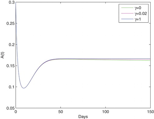
In order to evaluate the effect of media coverage on the dynamics of alcoholics, we choose different values of m, γ (see Figures  4 and 5). In Figure 4, we compare the density of alcoholic individuals with different values of m (0, 0.1, 0.3, 0.9), the simulation shows that the more implementation rate of media coverage, the lower the final alcoholics' density. On the contrary, in Figure 5, the more the depletion rate of media coverage, the higher the final alcoholics' density. So we know that the number of alcoholics will reduce substantially with the media coverage increasing.

Figure 4. The influence of different values of m on the population of alcoholics.

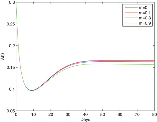
Figure 5. The influence of different values of γ on the population of alcoholics.

Now, we explore numerically an optimal control for the system (28(28) $\begin{array}{rl}\frac{\mathrm{d}P}{\mathrm{d}t}& =b-(1-u_1(t\left)\right)\beta (1-\frac{M}{k_0+M})PA-\mu P,\\ \frac{\mathrm{d}A}{\mathrm{d}t}& =(1-u_1(t\left)\right)\beta (1-\frac{M}{k_0+M})PA-q\frac{M}{k_1+M}A-(\mu +d)A-u_2\left(t\right)A,\\ \frac{\mathrm{d}Q}{\mathrm{d}t}& =q\frac{M}{k_1+M}A+u_2\left(t\right)A-\mu Q,\\ \frac{\mathrm{d}M}{\mathrm{d}t}& =mdA-\gamma M,\end{array}$(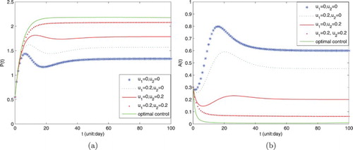28) ). To determine it, first, we choose $b_1=10$, $b_2=1$. Figure 6(a, b) indicate that the changes of population $P\left(t\right)$ and $A\left(t\right)$ with the different values of $u_1$, $u_2$. From Figure 6(a), we can easily get that the system with control is better than that without control. When $u_1=0$, $u_2=0$, $P\left(t\right)$ tends to a lowest value. When $u_1=0.2,u_2=0$ is better than $u_1=0,u_2=0.2$, and comparing with $u_1=0.2,u_2=0$, $u_1=0.2,u_2=0.2$ is better. From Figure 6(b), we know that the density of $A\left(t\right)$ decreases with the values of $u_1$ and $u_2$ increasing.

Figure 6. Variations of population with different control, where $b_1=10$, $b_2=1$.

If we change weight coefficients into $b_1=1$, $b_2=10$, we know that there is little difference between Figures  6(a, b) and 7(a, b). So we can draw the same conclusion.

Figure 7. Variations of population with different control, where $b_1=1$, $b_2=10$.

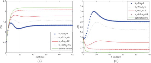
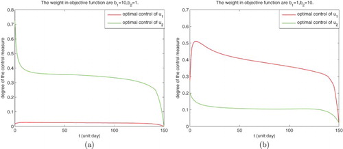
Figure 8 shows the process of control measure with different weight coefficients. In Figure  8(a), when we choose $b_1=10$, $b_2=1$, the simulation shows that the control $u_2$ starts from around 0.73, then it continues the slowly declining trend and finally toward a level of 0. But the control $u_1$ is relatively stable approaching to 0. In Figure8(b), we choose $b_1=1$, $b_2=10$, it's obvious that the control $u_1$ reaches peak about 0.51 at the time about 10, then it gradually decrease to 0 with the increase of time. As for the control $u_2$, it gradually reduces from 0.2 to 0.

Figure 8. The impact of different weight coefficients on optimal control $u_1$, $u_2$.

In this paper, we proposed an alcoholism model with media coverage. Unlike some of other previous model, we have taken into account the impact of media on alcoholics. First, we get the basic reproduction number $R_0$ by next generation matrix method. Second, we obtain that the alcohol free equilibrium of the model is globally asymptotically stable if $R_0<1$. For $R_0>1$, the alcohol present equilibrium is locally asymptotically stable. Next, we establish the optimality system and obtain the necessary condition of optimality by the Pontryagin's maximum principle. At last, we use numerical method to simulate outcomes which we have been proved.

Our results show that media coverage has substantial influence on the dynamics of alcoholics and can greatly influence the spread of the drinking, thus, it is crucial to educate people by media coverage to quit drinking.

Disclosure statement

No potential conflict of interest was reported by the authors.

Additional information

Funding

This work was partially supported by The National Natural Science Foundation of China [11461041 and 11661050], the Natural Science Foundation of Gansu Province of China [148RJZA024] and the development program for HongLiu Distinguished Young Scholars in Lanzhou University of Technology.

References

- N.G. Becker and D.N. Starczak, Optimal vaccination strategies for a community of households, Math. Biosci. 139 (1997), pp. 117–132.
- M.L. Brandeau, G.S. Zaric, and A. Richter, Resource allocation for control of infectious diseases in multiple independent populations: Beyond cost-effectiveness analysis, J. Health Econ. 22 (2003), pp. 575–598.
- Y. Cai, Y. Kang, M. Banerjee, and W. Wang, A stochastic SIRS epidemic model with infectious force under intervention strategies, J. Differ. Equ. 259 (2015), pp. 7463–7502.
- Y. Cai, Y. Kang, M. Banerjee, and W. Wang, A stochastic epidemic model incorporating media coverage, Commun. Math. Sci. 14 (2016), pp. 892–910.
- J.F. Cao, W.T. Li, and F.Y. Yang, Dynamics of a nonlocal SIS epidemic model with free boundary, Discrete Contin. Dyn. Syst. Ser. B 22 (2017), pp. 247–266.
- C. Castilho, Optimal control of an epidemic through educational campaign, Electron. J. Diff. Equ. 2006 (2006), pp. 1–11.
- P. van den Driessche and J. Watmough, Reproduction numbers and sub-threshold endemic equilibria for compartmental models of disease transmission, Math. Biosci. 180 (2002), pp. 29–48.
- W.H. Fleming and R.W. Rishel, Deterministic and Stochastic Optimal Control, Springer, Berlin, Germany, 1975.
- S. Ghosh, S. Guria, and M. Das, Alcohol as a risk factor for cancer burden: A review, Proc. Zoolog. Soc. 69 (2016), pp. 32–37.
- H.F. Huo and L.X. Feng, Global stability for an HIV/AIDS epidemic model with different latent stages and treatment, Appl. Math. Model. 37 (2013), pp. 1480–1489.
- H.F. Huo and X.M. Zhang, Complex dynamics in an alcoholism model with the impact of Twitter, Math. Biosci. 281 (2016), pp. 24–35.
- M. Kot, Elements of Mathematical Biology, Cambridge University Press, Cambridge, 2001.
- H. Laarabi, A. Abta, and K. Hattaf, Optimal control of a delayed SIRS epidemic model with vaccination and treatment, Acta Biotheor. 63 (2015), pp. 87–97.
- J.P. LaSalle, The Stability of Dynamical Systems, Regional Conference Series in Applied Mathematics, Society for Industrial and Applied Mathematics, Berlin, NJ, 1976.
- W. Lechner, A.M. Day, J. Metrik, A.M. Leventhal, and C.W. Kahler, Effects of alcohol-induced working memory decline on alcohol consumption and adverse consequences of use, Psychopharmacology 233 (2016), pp. 83–88.
- Y. Liu and J. Cui, The impact of media converage on the dynamics of infectious diseases, Int. J. Biomath. 1 (2008), pp. 65–74.
- R.S. Liu, J.H. Wu, and H.P. Zhu, Media/psychological impact on multiple outbreaks of emerging infectious disease, Comput. Math. Methods Med. 8 (2007), pp. 153–164.
- S.H. Ma, H.F. Huo and X.Y. Meng, Modelling alcoholism as a contagious disease: A mathematical model with awareness programs and time delay, Discrete Dynamics in Nature and Society, 2015, Article ID 260195, 13 pages.
- G. Mulone and B. Straughan, Modeling binge drinking, Int. J. Biomath. 5 (2012), pp. 57–70.
- S. Mushayabasa and C.P. Bhunu, Modelling the effects of heavy alcohol consumption on the transmission dynamics of gonorrhea, Nonlinear Dynam. 66 (2011), pp. 695–706.
- L.S. Pontryagin, V.G. Boltyanskii, R.V. Gamkrelidze, and E.F. Mishchenko, The Mathematical Theory of Optimal Processes, Interscience, New York, USA, 1965.
- J. Rehn, C. Mathers, S. Popova, M. Thavorncharoensap, Y. Teerawattananon, and J. Patra, Global burden of disease and injury and economic cost attributable to alcohol use and alcohol-use disorders, Lancet 373 (2009), pp. 2223–2233.
- S. Samanta, S. Rana, A. Sharma, A.K. Misra, and J. Chattopadhyay, Effect of awareness programs by media on the epidemic outbreaks: A mathematical model, Appl. Math. Comput. 219 (2013), pp. 6965–6977.
- F. Sanchez, X. Wang, C. Castillo-Chavez, D.M. Gorman, and P.J. Gruenewald, Drinking as an epidemica simple mathematical model with recovery and relapse, in Therapists Guide to Evidence-Based Relapse Prevention: Practical Resources for the Mental Health Professional, K.A. Witkiewitz and G.A. Marlatt, eds., Academic Press, Burlington, Canada, 2007, pp. 353–368.
- O. Sharomi and A.B. Gumel, Curtailing smoking dynamics: A mathematical modeling approach, Appl. Math. Comput. 195 (2008), pp. 475–499.
- R. Straus and S.D. Bacon, Drinking in College, Greenwood Press, New Haven, 1971.
- Y. Wang, J.D. Cao, Z. Jin, H.F. Zhang, and G.Q. Sun, Impact of media coverage on epidemic spreading in complex networks, Statist. Mech. Appl. 392 (2013), pp. 5824–5835.
- X.Y. Wang, K. Hattaf, H.F. Huo, and H. Xiang, Stability analysis of a delayed social epidemics model with general contact rate and its optimal control, J. Ind. Manag. Optim. 12 (2016), pp. 1267–1285.
- H. Xiang, L.X. Feng, and H.F. Huo, Stability of the virus dynamics model with Beddington-DeAngelis functional response and delays, Appl. Math. Model. 37 (2013), pp. 5414–5423.
- H. Xiang, Y.L. Tang, and H.F. Huo, A viral model with intracellular delay and humoral immunity, Bull. Malays. Math. Sci. Soc. (2016). doi: 10.1007/s40840-016-0326-2.
- G. Zaman, Qualitative behavior of giving up smoking models, Bull. Malays. Math. Sci. Soc. 34 (2009), pp. 403–415.
- G. Zaman, Optimal campaign in the smoking dynamics, Comput. Math. Methods Med. (2011), Article ID 163834, 9 pages.