Modelling and optimal control of pneumonia disease with cost-effective strategies

ABSTRACT

We propose and analyse a nonlinear mathematical model for the transmission dynamics of pneumonia disease in a population of varying size. The deterministic compartmental model is studied using stability theory of differential equations. The effective reproduction number is obtained and also the asymptotic stability conditions for the disease free and as well as for the endemic equilibria are established. The possibility of bifurcation of the model and the sensitivity indices of the basic reproduction number to the key parameters are determined. Using Pontryagin's maximum principle, the optimal control problem is formulated with three control strategies: namely disease prevention through education, treatment and screening. The cost-effectiveness analysis of the adopted control strategies revealed that the combination of prevention and treatment is the most cost-effective intervention strategies to combat the pneumonia pandemic. Numerical simulation is performed and pertinent results are displayed graphically.

Keywords:

• Pneumonia dynamics
• stability analysis
• optimal control
• cost-effectiveness analysis
• numerical simulation

1. Introduction

In the report of WHO [18], ‘infectious diseases are the leading cause of death in Human beings’. According to the fact sheet of WHO [18] sixteen percent of all deaths each year are from infectious diseases that means over 9.5 million deaths annually attribute to infectious diseases, with most of them in developing countries. From 9.5 million annual death, ‘Pneumonia and other respiratory infections cause about 2 million child deaths yearly in developing countries’ [19]. If we compare infectious diseases such as Malaria, HIV/AIDS, Measles and Pneumonia for under five-year children in Africa, pneumonia is the leading cause of deaths [19]. According to Institute for Health Metrics and Evaluation [4], every 35 seconds a child dies from pneumonia.

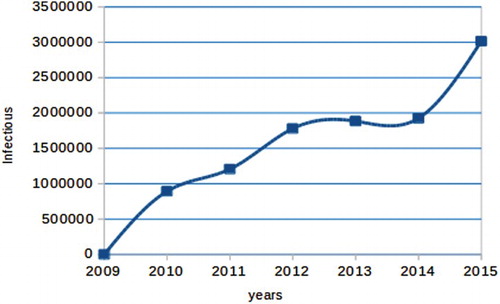
In Ethiopia, pneumonia is one of the leading cause of death. The reported cases shows that, it has been increasing aggregatively in the past 7 years (see Figure 1).

Figure 1. Reported cases of Pneumonia disease in Ethiopia from 2009 to 2015.

A lot of scholars proposed models for understanding of infectious disease dynamics and also for making quantitative predictions of different intervention strategies and their effectiveness [10–13]. Very few essential research have been done on the dynamics of pneumonia have been done in the last decade. Some of them are, Melegaro et al. [8], Joseph Emaline [5], Ssebuliba, [16] and Okaka et al. [9], proposed a model on pneumonia dynamics. Additionally, Ong'ala et al. [14] studied and estimated the basic reproductive number as a random variable by first developing and analysing a deterministic model for transmission patterns of pneumonia.

All the above studies have developed a deterministic as well as stochastic mathematical model of pneumonia dynamics by subdividing the population into sub-classes of susceptible, infectious, vaccinated, treated, carrier and recovered. But none of them considered optimal control and cost-effectiveness strategies and also no study have been undertaken by applying optimal control. This, therefore motivated us to undertake this study to fulfil this gap. To estimate some parameters demographic data were collected from Health Minster of federal democratic republic of Ethiopia.

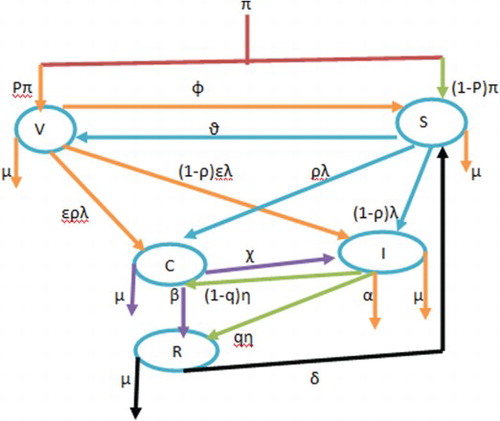
2. Model description and formulation

The model divides the total population into five sub-classes according to their disease status. Susceptible (S), vaccinated (V ), carrier (C), infected (I) and recovered (R). The model assumes that a fraction of the population has been vaccinated before the disease out break at the rate of $\left(p\right)$ and $(1-p)$ fraction of population susceptible. (We consider this model due to the reason that, in African particularly in Ethiopian context all new born infants are not taking Pneumococcal conjugate vaccine (PCV). Only those mothers who are aware or who stay around town or city will go to their nearby health centre to vaccinate their infants but there are a lot of newborn left without vaccination).The Susceptible class is increased from vaccinated class in which those individuals who are vaccinated but did not respond to vaccination with waning rate of φ and from recovered class in which those individuals who loss their temporary immunity by δ rate. However, individuals from susceptible class move to vaccinated class with vaccination rate of $\vartheta$. The susceptible class is infected either by carrier or symptomatically infected individuals with a force of infection $\lambda =\xi \left(\left(I\right(t)+\mathrm{{\rm Y}}C(t\left)\right)/N\right)$ where, $\xi =k\tau$, k is contact rate, τ is the probability that a contact is effective to cause infection and ϒ is transmission coefficient for the carrier. If $\mathrm{{\rm Y}}>1$ then, the carries infect susceptible more likely than infective. If $\mathrm{{\rm Y}}=1$, then both carriers and infective have equal chance to infect the susceptible, but if $\mathrm{{\rm Y}}<1$ then the infective have good chance to infect susceptible than carriers. The model assumes vaccination is not $100\mathrm{\%}$ effective, so vaccinated classes (V ) also have a chance of being infectious or carrier with small proportion and the force of infection for the vaccinated class is ${\lambda }_v=ϵ\lambda$, where $0\le ϵ<1$ and ε is the proportion of the serotype not covered by the vaccine. Newly infected individuals by the force of infection become either carrier with a probability of ρ to join the carrier class C or move to the infected class I with probability of $1-\rho$. The carrier class can develop disease symptom or can screen themselves and join the infected class with a rate of χ or recover by gaining natural immunity at β rate. Individuals in the infected class move to recovered compartment at a per capita rate of η by treatment, with treatment efficacy of q proportion of individuals join the recovered class or join the carrier class with $(1-q)$ proportion by adapting the treatment, or die from the disease at the rate α. In all compartments μ is the natural mortality rate of individuals and also all the parameters are positive. The above model description can be represented diagrammatically in Figure  2.

Figure 2. Flow diagram of the model.

The above flow diagram can be written in to a system of five differential equations as follows: (1) $\begin{array}{rl}\frac{\mathrm{d}S\left(t\right)}{\mathrm{d}t}& =(1-p)\pi +\phi V\left(t\right)+\delta R\left(t\right)-(\mu +\lambda +\vartheta )S\left(t\right),\\ \frac{\mathrm{d}V\left(t\right)}{\mathrm{d}t}& =p\pi +\vartheta S\left(t\right)-(\mu +ϵ\lambda +\phi )V\left(t\right),\\ \frac{\mathrm{d}C\left(t\right)}{\mathrm{d}t}& =\rho \lambda S\left(t\right)+\rho ϵ\lambda V\left(t\right)+(1-q)\eta I\left(t\right)-(\mu +\beta +\chi )C\left(t\right),\\ \frac{\mathrm{d}I\left(t\right)}{\mathrm{d}t}& =(1-\rho )\lambda S\left(t\right)+(1-\rho )ϵ\lambda V\left(t\right)+\chi C\left(t\right)-(\mu +\alpha +\eta )I\left(t\right),\\ \frac{\mathrm{d}R\left(t\right)}{\mathrm{d}t}& =\beta C\left(t\right)+q\eta I\left(t\right)-(\mu +\delta )R\left(t\right).\end{array}$(1) With initial condition $S\left(0\right)=S_0$, $V\left(0\right)=V_0$, $I\left(0\right)=I_0$, $C\left(0\right)=C_0$, $R\left(0\right)=R_0$.

3. Model analysis

3.1. Invariant region

In this section, a region in which solutions of the model system are uniformly bounded is the proper subset $\mathrm{\Omega }\subset {\mathrm{\Re }}_{+}^5$.

The total population at any time t is given by N=S+V +C+I+R. and $\mathrm{d}N/\mathrm{d}t=\pi -\mu N-\alpha I\left(t\right)$.

In the absence of mortality due to pneumonia equation, it becomes (2) $\frac{\mathrm{d}N}{\mathrm{d}t}\le \pi -\mu N.$(2) By solving Equation (2(2) $\frac{\mathrm{d}N}{\mathrm{d}t}\le \pi -\mu N.$(2) ), we obtain $0\le N\le \pi /\mu$. Therefore, the feasible solution set of the system equation  (1(1) $\begin{array}{rl}\frac{\mathrm{d}S\left(t\right)}{\mathrm{d}t}& =(1-p)\pi +\phi V\left(t\right)+\delta R\left(t\right)-(\mu +\lambda +\vartheta )S\left(t\right),\\ \frac{\mathrm{d}V\left(t\right)}{\mathrm{d}t}& =p\pi +\vartheta S\left(t\right)-(\mu +ϵ\lambda +\phi )V\left(t\right),\\ \frac{\mathrm{d}C\left(t\right)}{\mathrm{d}t}& =\rho \lambda S\left(t\right)+\rho ϵ\lambda V\left(t\right)+(1-q)\eta I\left(t\right)-(\mu +\beta +\chi )C\left(t\right),\\ \frac{\mathrm{d}I\left(t\right)}{\mathrm{d}t}& =(1-\rho )\lambda S\left(t\right)+(1-\rho )ϵ\lambda V\left(t\right)+\chi C\left(t\right)-(\mu +\alpha +\eta )I\left(t\right),\\ \frac{\mathrm{d}R\left(t\right)}{\mathrm{d}t}& =\beta C\left(t\right)+q\eta I\left(t\right)-(\mu +\delta )R\left(t\right).\end{array}$(1) ) of the model remain in the region: (3) $\mathrm{\Omega }=\left\{(S,V,C,I,R)\in {\mathrm{\Re }}_{+}^5:N\le \frac{\pi }{\mu }\right\}.$(3)

3.2. Positivity of the solutions

In this section, to obtain the solution of the model is non-negative we stated and proved the following theorem.

Theorem 3.1

let $\mathrm{\Omega }=\left\{\right(S,V,C,I,R)\in {\mathrm{\Re }}_{+}^5:S_0>0,V_0>0,C_0>0,I_0>0,R_0>0\}$, then the solution of $\{S,V,C,I,R\}$ are positive for $t\ge 0$.

Proof.

From the system of differential equation (1(1) $\begin{array}{rl}\frac{\mathrm{d}S\left(t\right)}{\mathrm{d}t}& =(1-p)\pi +\phi V\left(t\right)+\delta R\left(t\right)-(\mu +\lambda +\vartheta )S\left(t\right),\\ \frac{\mathrm{d}V\left(t\right)}{\mathrm{d}t}& =p\pi +\vartheta S\left(t\right)-(\mu +ϵ\lambda +\phi )V\left(t\right),\\ \frac{\mathrm{d}C\left(t\right)}{\mathrm{d}t}& =\rho \lambda S\left(t\right)+\rho ϵ\lambda V\left(t\right)+(1-q)\eta I\left(t\right)-(\mu +\beta +\chi )C\left(t\right),\\ \frac{\mathrm{d}I\left(t\right)}{\mathrm{d}t}& =(1-\rho )\lambda S\left(t\right)+(1-\rho )ϵ\lambda V\left(t\right)+\chi C\left(t\right)-(\mu +\alpha +\eta )I\left(t\right),\\ \frac{\mathrm{d}R\left(t\right)}{\mathrm{d}t}& =\beta C\left(t\right)+q\eta I\left(t\right)-(\mu +\delta )R\left(t\right).\end{array}$(1) ), let us take the first equation; $\begin{array}{rl}\frac{\mathrm{d}S}{\mathrm{d}t}& =(1-p\psi )\pi +\phi V+\delta R-(\mu +\lambda +\vartheta )S\\ & \Rightarrow \frac{\mathrm{d}S}{\mathrm{d}t}\ge -(\mu +\lambda +\vartheta )S\\ & \Rightarrow \frac{\mathrm{d}S}{S}\ge -(\mu +\lambda +\vartheta )\mathrm{d}\left(t\right)\\ & \Rightarrow \int \frac{\mathrm{d}S}{S}\ge -\int (\mu +\lambda +\vartheta )\mathrm{d}\left(t\right)\\ S\left(t\right)& \ge S_0\exp -(\mu +\lambda +\vartheta )t\ge 0.\end{array}$ Similarly, we obtained $\begin{array}{rl}V\left(t\right)& \ge V_0\exp -(\mu +ϵ\lambda +\phi )t\ge 0.\\ C\left(t\right)& \ge C_0\exp -(\mu +\beta +\chi )t\ge 0.\\ I\left(t\right)& \ge I_0\exp -(\mu +\alpha +\eta )t\ge 0.\\ R\left(t\right)& \ge R_0\exp -(\mu +\alpha +(1-q\left)\eta \right)t\ge 0.\end{array}$

3.3. Disease-free equilibrium

In this section we obtain the equilibrium point at which the epidemic is eradicated from the population. Letting the right-hand side of Equation (1(1) $\begin{array}{rl}\frac{\mathrm{d}S\left(t\right)}{\mathrm{d}t}& =(1-p)\pi +\phi V\left(t\right)+\delta R\left(t\right)-(\mu +\lambda +\vartheta )S\left(t\right),\\ \frac{\mathrm{d}V\left(t\right)}{\mathrm{d}t}& =p\pi +\vartheta S\left(t\right)-(\mu +ϵ\lambda +\phi )V\left(t\right),\\ \frac{\mathrm{d}C\left(t\right)}{\mathrm{d}t}& =\rho \lambda S\left(t\right)+\rho ϵ\lambda V\left(t\right)+(1-q)\eta I\left(t\right)-(\mu +\beta +\chi )C\left(t\right),\\ \frac{\mathrm{d}I\left(t\right)}{\mathrm{d}t}& =(1-\rho )\lambda S\left(t\right)+(1-\rho )ϵ\lambda V\left(t\right)+\chi C\left(t\right)-(\mu +\alpha +\eta )I\left(t\right),\\ \frac{\mathrm{d}R\left(t\right)}{\mathrm{d}t}& =\beta C\left(t\right)+q\eta I\left(t\right)-(\mu +\delta )R\left(t\right).\end{array}$(1) ) to zero and letting C=I=0, leads to $E_0=\left(\frac{\pi }{\mu }\mathrm{\wp },\frac{\pi }{\mu }\mathrm{\Im },0,0,0\right),$ where $\mathrm{\wp }=(\mu -P\pi \mu +\phi )/(\mu +\phi +\vartheta )$ and $\mathrm{\Im }=(P\pi \mu +\vartheta )/(\mu +\phi +\vartheta )$.

3.4. The effective reproductive number ($R_{\mathrm{eff}}$)

In this section we obtained the threshold parameter that governs the spread of a disease which is called the effective reproduction number is determined. To obtain the effective reproduction number, we used the next-generation matrix method so that it is the spectral radius of the next-generation matrix [17] and we obtain (4) $\begin{array}{rl}{R}_{\mathrm{eff}}& =k\tau \left[\frac{\rho \left(\mathrm{{\rm Y}}\right(\mu +\alpha +\eta )+\chi )}{(\mu +\beta +\chi )(\mu +\alpha +\eta )-\chi \eta (1-q)}\right.\\ & +\left.\frac{(1-\rho )\left(\mathrm{{\rm Y}}\right(1-q)\eta +(\mu +\beta +\chi \left)\right)}{(\mu +\beta +\chi )(\mu +\alpha +\eta )-\chi \eta (1-q)}\right]\left(\frac{\pi }{\mu }\mathrm{\wp }+ϵ\frac{\pi }{\mu }\mathrm{\Im }\right).\end{array}$(4)

3.5. Local stability of disease-free equilibrium

Theorem 3.2

The disease-free equilibrium point is locally asymptotically stable if $R_{\mathrm{eff}}<1$ and unstable if $R_{\mathrm{eff}}>1$.

Proof.

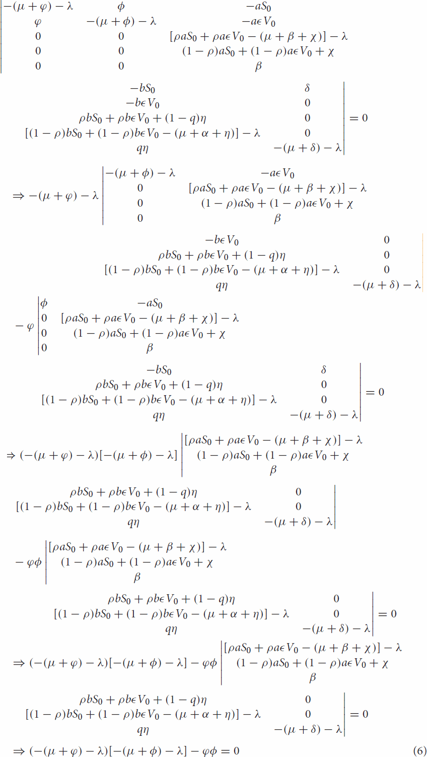
To prove local stability of disease-free equilibrium, we obtained the Jacobian matrix of the system (1(1) $\begin{array}{rl}\frac{\mathrm{d}S\left(t\right)}{\mathrm{d}t}& =(1-p)\pi +\phi V\left(t\right)+\delta R\left(t\right)-(\mu +\lambda +\vartheta )S\left(t\right),\\ \frac{\mathrm{d}V\left(t\right)}{\mathrm{d}t}& =p\pi +\vartheta S\left(t\right)-(\mu +ϵ\lambda +\phi )V\left(t\right),\\ \frac{\mathrm{d}C\left(t\right)}{\mathrm{d}t}& =\rho \lambda S\left(t\right)+\rho ϵ\lambda V\left(t\right)+(1-q)\eta I\left(t\right)-(\mu +\beta +\chi )C\left(t\right),\\ \frac{\mathrm{d}I\left(t\right)}{\mathrm{d}t}& =(1-\rho )\lambda S\left(t\right)+(1-\rho )ϵ\lambda V\left(t\right)+\chi C\left(t\right)-(\mu +\alpha +\eta )I\left(t\right),\\ \frac{\mathrm{d}R\left(t\right)}{\mathrm{d}t}& =\beta C\left(t\right)+q\eta I\left(t\right)-(\mu +\delta )R\left(t\right).\end{array}$(1) ) at the disease-free equilibrium $E_0$: (5) $\begin{array}{rl}J(S_0,V_0,0,0,0)& =\left[\begin{array}{ccc}-(\mu +\varphi )& \phi & -a{S}_0\\ \varphi & -(\mu +\phi )& -aϵV_0\\ 0& 0& \rho a{S}_0+\rho aϵV_0-(\mu +\beta +\chi )\\ 0& 0& (1-\rho )a{S}_0+(1-\rho )aϵV_0+\chi \\ 0& 0& \beta \end{array}\right.\\ & \left.\begin{array}{cc}-b{S}_0& \delta \\ -bϵV_0& 0\\ \rho b{S}_0+\rho bϵV_0+(1-q)\eta & 0\\ (1-\rho )b{S}_0+(1-\rho )bϵV_0-(\mu +\alpha +\eta )& 0\\ q\eta & -(\mu +\delta )\end{array}\right].\end{array}$(5) To obtain the eigenvalue of Equation (5(5) $\begin{array}{rl}J(S_0,V_0,0,0,0)& =\left[\begin{array}{ccc}-(\mu +\varphi )& \phi & -a{S}_0\\ \varphi & -(\mu +\phi )& -aϵV_0\\ 0& 0& \rho a{S}_0+\rho aϵV_0-(\mu +\beta +\chi )\\ 0& 0& (1-\rho )a{S}_0+(1-\rho )aϵV_0+\chi \\ 0& 0& \beta \end{array}\right.\\ & \left.\begin{array}{cc}-b{S}_0& \delta \\ -bϵV_0& 0\\ \rho b{S}_0+\rho bϵV_0+(1-q)\eta & 0\\ (1-\rho )b{S}_0+(1-\rho )bϵV_0-(\mu +\alpha +\eta )& 0\\ q\eta & -(\mu +\delta )\end{array}\right].\end{array}$(5) ), or when we expand Equation (6) (8) ${\lambda }^2+(2\mu +\phi +\varphi )\lambda +\mu (\mu +\phi +\varphi ).$(8) Then by Routh–Hurwitz criteria equation  (8(8) ${\lambda }^2+(2\mu +\phi +\varphi )\lambda +\mu (\mu +\phi +\varphi ).$(8) ) have strictly negative root.

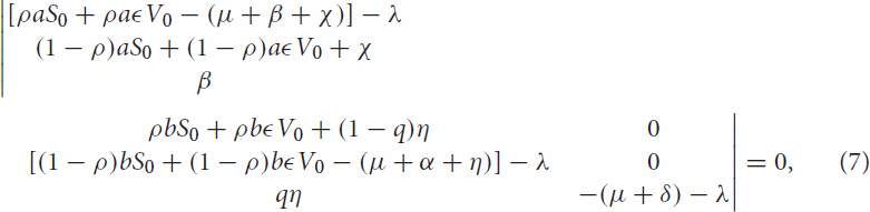
The determinant of Equation (7) can be obtained $\begin{array}{rl}& \left|\begin{array}{ccc}\rho a(S_0+ϵV_0)-(\mu +\beta +\chi )-\lambda & \rho b(S_0+ϵV_0)+(1-q)\eta & 0\\ (1-\rho )a(S_0+ϵV_0)+\chi & (1-\rho )b(S_0+ϵV_0)-(\mu +\alpha +\eta )-\lambda & 0\\ \beta & q\eta & -(\mu +\delta )-\lambda \end{array}\right|=0\\ & \Rightarrow -(\mu +\delta )-\lambda \left|\begin{array}{cc}\rho a(S_0+ϵV_0)-(\mu +\beta +\chi )-\lambda & \rho b(S_0+ϵV_0)+(1-q)\eta \\ (1-\rho )a(S_0+ϵV_0)+\chi & (1-\rho )b(S_0+ϵV_0)-(\mu +\alpha +\eta )-\lambda \end{array}\right|=0,\end{array}$

then ${\lambda }_1=-(\mu +\delta )<0$ and (9) $\begin{array}{rl}& \left(\rho a\right(S_0+ϵV_0)-(\mu +\beta +\chi )-\lambda )\left(\right(1-\rho \left)b\right(S_0+ϵV_0)-(\mu +\alpha +\eta )-\lambda )\\ & -\left(\right(1-\rho \left)a\right(S_0+ϵV_0)+\chi )\left(\rho b\right(S_0+ϵV_0)+(1-q\left)\eta \right)=0,\end{array}$(9) when we rearrange Equation (9(9) $\begin{array}{rl}& \left(\rho a\right(S_0+ϵV_0)-(\mu +\beta +\chi )-\lambda )\left(\right(1-\rho \left)b\right(S_0+ϵV_0)-(\mu +\alpha +\eta )-\lambda )\\ & -\left(\right(1-\rho \left)a\right(S_0+ϵV_0)+\chi )\left(\rho b\right(S_0+ϵV_0)+(1-q\left)\eta \right)=0,\end{array}$(9) ), it becomes ${\lambda }^2+a_1\lambda +a_2=0,$ where $\begin{array}{rl}{a}_1& =(\mu +\beta +\chi )+(\mu +\alpha +\eta )-(\rho a+(1-\rho \left)b\right)(S_0+ϵV_0),\\ a_2& =-\left(\rho \right(a(\mu +\alpha +\eta )+b\chi )+(1-\rho \left)\right(b(\mu +\beta +\chi )+a(1-q)\eta \left)\right)(S_0+ϵV_0)\\ & -\left(\right(1-q)\chi \eta -(\mu +\beta +\chi \left)\right(\mu +\alpha +\eta \left)\right).\end{array}$ By Routh–Hurwitz criteria, $a_1>0$ means that, $(\mu +\beta +\chi )+(\mu +\alpha +\eta )>(\rho a+(1-\rho \left)b\right)(S_0+ϵV_0),$ and also $a_2>0$ means that, $\begin{array}{rl}& -\left(\rho \right(a(\mu +\alpha +\eta )+b\chi )+(1-\rho \left)\right(b(\mu +\beta +\chi )+a(1-q)\eta \left)\right)(S_0+ϵV_0)\\ & -\left(\right(1-q)\chi \eta -(\mu +\beta +\chi \left)\right(\mu +\alpha +\eta \left)\right)>0\\ & \Rightarrow \left[\right(\rho \left(a\right(\mu +\alpha +\eta )+b\chi )+(1-\rho )\left(b\right(\mu +\beta +\chi )+a(1-q\left)\eta \right)\left)\right](S_0+ϵV_0)\\ & <(\mu +\beta +\chi )(\mu +\alpha +\eta )-(1-q)\chi \eta \\ & \Rightarrow \frac{\left[\right(\rho \left(a\right(\mu +\alpha +\eta )+b\chi )+(1-\rho )\left(b\right(\mu +\beta +\chi )+a(1-q\left)\eta \right)\left)\right]}{(\mu +\beta +\chi )(\mu +\alpha +\eta )-(1-q)\chi \eta }\left(S_0+ϵV_0\right)<1\\ & \Rightarrow R_{\mathrm{eff}}<1,\end{array}$ Thus, the disease-free equilibrium is locally asymptotically stable if $R_{\mathrm{eff}}<1$.

3.6. The endemic equilibrium

The endemic equilibrium is denoted by $E^{\ast }$ and defined as a steady-state solutions for the model (1(1) $\begin{array}{rl}\frac{\mathrm{d}S\left(t\right)}{\mathrm{d}t}& =(1-p)\pi +\phi V\left(t\right)+\delta R\left(t\right)-(\mu +\lambda +\vartheta )S\left(t\right),\\ \frac{\mathrm{d}V\left(t\right)}{\mathrm{d}t}& =p\pi +\vartheta S\left(t\right)-(\mu +ϵ\lambda +\phi )V\left(t\right),\\ \frac{\mathrm{d}C\left(t\right)}{\mathrm{d}t}& =\rho \lambda S\left(t\right)+\rho ϵ\lambda V\left(t\right)+(1-q)\eta I\left(t\right)-(\mu +\beta +\chi )C\left(t\right),\\ \frac{\mathrm{d}I\left(t\right)}{\mathrm{d}t}& =(1-\rho )\lambda S\left(t\right)+(1-\rho )ϵ\lambda V\left(t\right)+\chi C\left(t\right)-(\mu +\alpha +\eta )I\left(t\right),\\ \frac{\mathrm{d}R\left(t\right)}{\mathrm{d}t}& =\beta C\left(t\right)+q\eta I\left(t\right)-(\mu +\delta )R\left(t\right).\end{array}$(1) ). This can occur when there is a persistence of the disease. It can be obtained by equating the system of Equation (1(1) $\begin{array}{rl}\frac{\mathrm{d}S\left(t\right)}{\mathrm{d}t}& =(1-p)\pi +\phi V\left(t\right)+\delta R\left(t\right)-(\mu +\lambda +\vartheta )S\left(t\right),\\ \frac{\mathrm{d}V\left(t\right)}{\mathrm{d}t}& =p\pi +\vartheta S\left(t\right)-(\mu +ϵ\lambda +\phi )V\left(t\right),\\ \frac{\mathrm{d}C\left(t\right)}{\mathrm{d}t}& =\rho \lambda S\left(t\right)+\rho ϵ\lambda V\left(t\right)+(1-q)\eta I\left(t\right)-(\mu +\beta +\chi )C\left(t\right),\\ \frac{\mathrm{d}I\left(t\right)}{\mathrm{d}t}& =(1-\rho )\lambda S\left(t\right)+(1-\rho )ϵ\lambda V\left(t\right)+\chi C\left(t\right)-(\mu +\alpha +\eta )I\left(t\right),\\ \frac{\mathrm{d}R\left(t\right)}{\mathrm{d}t}& =\beta C\left(t\right)+q\eta I\left(t\right)-(\mu +\delta )R\left(t\right).\end{array}$(1) ) to zero. Then we obtained $\begin{array}{rl}{S}^{\ast }& =\frac{\begin{array}{c}(\mu +\beta +\chi )\left(\right(1-\rho \left)\right(1-q)\eta +\rho (\mu +\alpha +\eta \left)\right)\\ -(1-q)\eta \left(\right(1-\rho \left)\right(\mu +\beta +\chi )+\rho \chi )(\mu +ϵ\lambda +\phi )I^{\ast }\end{array}}{\left(\right((1-\rho )(\mu +\beta +\chi )+\rho \chi \left)\right(\mu +\delta \left)\right)\rho \lambda (\mu +ϵ\lambda +\phi +ϵ\vartheta )}.\\ V^{\ast }& =\frac{p\mathrm{\Psi }\pi +\vartheta S^{\ast }}{\mu +ϵ{\lambda }^{\ast }+\phi }.\\ C^{\ast }& =\frac{(1-\rho )(1-q)\eta +\rho (\mu +\alpha +\eta )}{(1-\rho )(\mu +\beta +\chi )+\rho \chi }{I}^{\ast },\\ I^{\ast }& =\frac{\begin{array}{c}{A}_2{\lambda }^{\ast \ast }({{\lambda }^{\ast \ast }}^2{ϵ}^2{D}_2+{\lambda }^{\ast \ast }\mu ϵD_2+{\lambda }^{\ast \ast }ϵD_2+{\lambda }^{\ast \ast }ϵD_2{D}_6+{\lambda }^{\ast \ast }ϵD_4+\mu D_2{D}_6\\ +\phi D_2{D}_6-{\lambda }^{\ast \ast }{D}_2+D_1{D}_7+D_4{D}_6)\end{array}}{\begin{array}{c}{A}_1\left({\lambda }^{\ast \ast }ϵD_5\right)D_7-\delta {{\lambda }^{\ast \ast }}^3{A}_5{A}_2{ϵ}^2+\delta {{\lambda }^{\ast \ast }}^2{D}_6{A}_5{A}_2ϵ+\delta {{\lambda }^{\ast \ast }}^2{D}_5{A}_5ϵ\\ +\delta {\lambda }^{\ast \ast }{D}_6{D}_5{A}_5{A}_2+A_1({\lambda }^{\ast \ast }ϵ+D_5){\lambda }^{\ast \ast }\end{array}}.\\ R^{\ast }& =\frac{\beta \left(\right(1-\rho \left)\right(1-q)\eta +\rho (\mu +\alpha +\eta \left)\right)+\left(\right(1-\rho \left)\right(\mu +\beta +\chi )+\rho \chi )q\eta }{\left(\right(1-\rho \left)\right(\mu +\beta +\chi )+\rho \chi )(\mu +\delta )}{I}^{\ast }.\end{array}$ where $\begin{array}{rl}{A}_1& =(\mu +\beta +\chi )\left(\right(\mu +\alpha +\eta )-\eta (1-q\left)\right),\\ A_2& =\chi \rho +(1-\rho )(\mu +\beta +\chi ),\\ A_3& =\rho (\mu +\delta {)}^2(\chi +(1-\rho )(\mu +\beta +\chi )),\\ A_4& =(\chi \rho +(1-\rho \left)\right)(\mu +\delta ),\\ A_5& =(1-\rho )\eta (1-q)+\rho (\mu +\alpha +\eta )+(\chi \rho +(1-\rho \left)\right(\mu +\beta +\chi \left)\right)q\eta ,\\ D_1& =ϵp\mathrm{\Psi }\pi ,\\ D_2& =A_3(1-p\mathrm{\Psi })\pi ,\\ D_4& =A_3\phi p\mathrm{\Psi }\pi ,\\ D_5& =\mu +\phi ,\\ D_6& =ϵ\vartheta +\mu +\phi ,\\ D_7& =A_4\phi \vartheta -\mu -\vartheta .\end{array}$ Hence $E^{\ast }=(S^{\ast },V^{\ast },C^{\ast },I^{\ast },R^{\ast })$ is the endemic equilibrium of the model 1(1) $\begin{array}{rl}\frac{\mathrm{d}S\left(t\right)}{\mathrm{d}t}& =(1-p)\pi +\phi V\left(t\right)+\delta R\left(t\right)-(\mu +\lambda +\vartheta )S\left(t\right),\\ \frac{\mathrm{d}V\left(t\right)}{\mathrm{d}t}& =p\pi +\vartheta S\left(t\right)-(\mu +ϵ\lambda +\phi )V\left(t\right),\\ \frac{\mathrm{d}C\left(t\right)}{\mathrm{d}t}& =\rho \lambda S\left(t\right)+\rho ϵ\lambda V\left(t\right)+(1-q)\eta I\left(t\right)-(\mu +\beta +\chi )C\left(t\right),\\ \frac{\mathrm{d}I\left(t\right)}{\mathrm{d}t}& =(1-\rho )\lambda S\left(t\right)+(1-\rho )ϵ\lambda V\left(t\right)+\chi C\left(t\right)-(\mu +\alpha +\eta )I\left(t\right),\\ \frac{\mathrm{d}R\left(t\right)}{\mathrm{d}t}& =\beta C\left(t\right)+q\eta I\left(t\right)-(\mu +\delta )R\left(t\right).\end{array}$(1) .

Lemma 3.3

For $R_{\mathrm{eff}}>1$ a unique endemic equilibrium point $E^{\ast }$ exist and no endemic equilibrium otherwise.

Proof.

For the disease to endemic, $\mathrm{d}C/\mathrm{d}t>0$ and $\mathrm{d}I/\mathrm{d}t>0$, that is: (10) $\begin{array}{rl}\frac{\mathrm{d}C\left(t\right)}{\mathrm{d}t}& =\rho \lambda S\left(t\right)+\rho ϵ\lambda V\left(t\right)+(1-q)\eta I\left(t\right)-(\mu +\beta +\chi )C\left(t\right)>0,\\ \frac{\mathrm{d}I\left(t\right)}{\mathrm{d}t}& =(1-\rho )\lambda S\left(t\right)+(1-\rho )ϵ\lambda V\left(t\right)+\chi C\left(t\right)-(\mu +\alpha +\eta )I\left(t\right)>0.\end{array}$(10) From the second inequality of Equation (10(10) $\begin{array}{rl}\frac{\mathrm{d}C\left(t\right)}{\mathrm{d}t}& =\rho \lambda S\left(t\right)+\rho ϵ\lambda V\left(t\right)+(1-q)\eta I\left(t\right)-(\mu +\beta +\chi )C\left(t\right)>0,\\ \frac{\mathrm{d}I\left(t\right)}{\mathrm{d}t}& =(1-\rho )\lambda S\left(t\right)+(1-\rho )ϵ\lambda V\left(t\right)+\chi C\left(t\right)-(\mu +\alpha +\eta )I\left(t\right)>0.\end{array}$(10) ), $\begin{array}{rl}& (\mu +\alpha +\eta )I\left(t\right)<(1-\rho )\lambda S\left(t\right)+(1-\rho )ϵ\lambda V\left(t\right)+\chi C\left(t\right)\\ & \Rightarrow I<\frac{(1-\rho )\xi \left(\frac{I\left(t\right)+\mathrm{{\rm Y}}C\left(t\right)}{N}\right.(S+ϵV)+\chi C}{(\mu +\alpha +\eta )}\end{array}$ From the fact $(S+ϵV)/N\le 1$, (11) $I<\frac{(1-\rho )\xi I\left(t\right)+(1-\rho )\xi \mathrm{{\rm Y}}C\left(t\right)+\chi C}{(\mu +\alpha +\eta )}.$(11) From the first inequality of Equation (10(10) $\begin{array}{rl}\frac{\mathrm{d}C\left(t\right)}{\mathrm{d}t}& =\rho \lambda S\left(t\right)+\rho ϵ\lambda V\left(t\right)+(1-q)\eta I\left(t\right)-(\mu +\beta +\chi )C\left(t\right)>0,\\ \frac{\mathrm{d}I\left(t\right)}{\mathrm{d}t}& =(1-\rho )\lambda S\left(t\right)+(1-\rho )ϵ\lambda V\left(t\right)+\chi C\left(t\right)-(\mu +\alpha +\eta )I\left(t\right)>0.\end{array}$(10) ), $\begin{array}{rl}& (\mu +\beta +\chi )C\left(t\right)<\rho \lambda S\left(t\right)+\rho ϵ\lambda V\left(t\right)+(1-q)\eta I\left(t\right)\\ & \Rightarrow C<\frac{\rho \xi \left(\frac{I\left(t\right)+\mathrm{{\rm Y}}C\left(t\right)}{N}\right.(S+ϵV)+(1-q)\eta I\left(t\right)}{(\mu +\beta +\chi )}.\end{array}$ From the fact $(S+ϵV)/N\le 1$, (12) $C<\frac{\rho \xi I\left(t\right)+(1-q)\eta I\left(t\right)}{(\mu +\beta +\chi )-\rho \xi \mathrm{{\rm Y}}}.$(12) By substituting Equation (12(12) $C<\frac{\rho \xi I\left(t\right)+(1-q)\eta I\left(t\right)}{(\mu +\beta +\chi )-\rho \xi \mathrm{{\rm Y}}}.$(12) ) into Equation (11(11) $I<\frac{(1-\rho )\xi I\left(t\right)+(1-\rho )\xi \mathrm{{\rm Y}}C\left(t\right)+\chi C}{(\mu +\alpha +\eta )}.$(11) ) we can get, $I<\frac{(1-\rho )\xi I\left(\right(\mu +\beta +\chi )-\rho \xi \mathrm{{\rm Y}})+(1-\rho )\xi \mathrm{{\rm Y}}(\rho \xi I+(1-q\left)\eta I\right)+\chi (\rho \xi I+(1-q\left)\eta I\right)}{(\mu +\alpha +\eta )(\mu +\beta +\chi -\rho \xi \mathrm{{\rm Y}})}.$ Then, by rearranging and cancelling of I in both sides, we can get (13) $\begin{array}{rl}1& <\xi \left[\frac{\rho \left(\mathrm{{\rm Y}}\right(\mu +\alpha +\eta )+\chi )}{(\mu +\beta +\chi )(\mu +\alpha +\eta )-\chi \eta (1-q)}+\frac{(1-\rho )\left(\mathrm{{\rm Y}}\right(1-q)\eta +(\mu +\beta +\chi \left)\right)}{(\mu +\beta +\chi )(\mu +\alpha +\eta )-\chi \eta (1-q)}\right]\\ & \le \xi \left[\frac{\rho \left(\mathrm{{\rm Y}}\right(\mu +\alpha +\eta )+\chi )}{(\mu +\beta +\chi )(\mu +\alpha +\eta )-\chi \eta (1-q)}+\frac{(1-\rho )\left(\mathrm{{\rm Y}}\right(1-q)\eta +(\mu +\beta +\chi \left)\right)}{(\mu +\beta +\chi )(\mu +\alpha +\eta )-\chi \eta (1-q)}\right]\\ & \times \left(\frac{\pi }{\mu }\mathrm{\wp }+ϵ\frac{\pi }{\mu }\mathrm{\Im }\right)=R_{\mathrm{eff}}\\ & \Rightarrow 1<R_{\mathrm{eff}}.\end{array}$(13) Thus a unique endemic equilibrium exist when $R_{\mathrm{eff}}>1$.

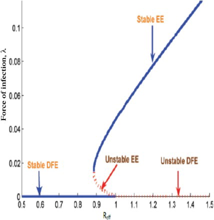
Using expression for $I^{\ast }$ in the endemic equilibrium, we plot Figure 10, that shows there is a backward bifurcation. We used a set of estimated parameters in Table 2. The figure reflects the co-existence of the disease free with endemic equilibrium.

3.7. Local stability of the endemic equilibrium

Theorem 3.4

If $R_{\mathrm{eff}}>1$ then the endemic equilibrium $E^{\ast }$ of system (1(1) $\begin{array}{rl}\frac{\mathrm{d}S\left(t\right)}{\mathrm{d}t}& =(1-p)\pi +\phi V\left(t\right)+\delta R\left(t\right)-(\mu +\lambda +\vartheta )S\left(t\right),\\ \frac{\mathrm{d}V\left(t\right)}{\mathrm{d}t}& =p\pi +\vartheta S\left(t\right)-(\mu +ϵ\lambda +\phi )V\left(t\right),\\ \frac{\mathrm{d}C\left(t\right)}{\mathrm{d}t}& =\rho \lambda S\left(t\right)+\rho ϵ\lambda V\left(t\right)+(1-q)\eta I\left(t\right)-(\mu +\beta +\chi )C\left(t\right),\\ \frac{\mathrm{d}I\left(t\right)}{\mathrm{d}t}& =(1-\rho )\lambda S\left(t\right)+(1-\rho )ϵ\lambda V\left(t\right)+\chi C\left(t\right)-(\mu +\alpha +\eta )I\left(t\right),\\ \frac{\mathrm{d}R\left(t\right)}{\mathrm{d}t}& =\beta C\left(t\right)+q\eta I\left(t\right)-(\mu +\delta )R\left(t\right).\end{array}$(1) ) is locally asymptotically stable in Ω.

Proof.

To Prove the local stability of endemic equilibrium, we obtain the Jacobian matrix at endemic equilibrium in Equation (14(14) $\begin{array}{rl}{J}_{E^{\ast }}& =J(S^{\ast },V^{\ast },C^{\ast },C^{\ast },R^{\ast })\\ & =\left[\begin{array}{ccccc}-(\mu +\overline{\lambda }+\varphi )& \phi & 0& 0& \delta \\ \varphi & -(\mu +ϵ\overline{\lambda }+\phi )& 0& 0& 0\\ \rho \overline{\lambda }& \rho ϵ\overline{\lambda }& -(\mu +\beta +\chi )& (1-q)\eta & 0\\ (1-\rho )\overline{\lambda }& (1-\rho )ϵ\overline{\lambda }& \chi & -(\mu +\alpha +\eta )& 0\\ 0& 0& \beta & q\eta & -(\mu +\delta )\end{array}\right].\end{array}$(14) ): (14) $\begin{array}{rl}{J}_{E^{\ast }}& =J(S^{\ast },V^{\ast },C^{\ast },C^{\ast },R^{\ast })\\ & =\left[\begin{array}{ccccc}-(\mu +\overline{\lambda }+\varphi )& \phi & 0& 0& \delta \\ \varphi & -(\mu +ϵ\overline{\lambda }+\phi )& 0& 0& 0\\ \rho \overline{\lambda }& \rho ϵ\overline{\lambda }& -(\mu +\beta +\chi )& (1-q)\eta & 0\\ (1-\rho )\overline{\lambda }& (1-\rho )ϵ\overline{\lambda }& \chi & -(\mu +\alpha +\eta )& 0\\ 0& 0& \beta & q\eta & -(\mu +\delta )\end{array}\right].\end{array}$(14) The characteristic polynomial of Equation (14(14) $\begin{array}{rl}{J}_{E^{\ast }}& =J(S^{\ast },V^{\ast },C^{\ast },C^{\ast },R^{\ast })\\ & =\left[\begin{array}{ccccc}-(\mu +\overline{\lambda }+\varphi )& \phi & 0& 0& \delta \\ \varphi & -(\mu +ϵ\overline{\lambda }+\phi )& 0& 0& 0\\ \rho \overline{\lambda }& \rho ϵ\overline{\lambda }& -(\mu +\beta +\chi )& (1-q)\eta & 0\\ (1-\rho )\overline{\lambda }& (1-\rho )ϵ\overline{\lambda }& \chi & -(\mu +\alpha +\eta )& 0\\ 0& 0& \beta & q\eta & -(\mu +\delta )\end{array}\right].\end{array}$(14) ) in terms of force of infection is obtained as $P\left(\lambda \right)={\lambda }^5+Z_1{\lambda }^4+Z_2{\lambda }^3+Z_3{\lambda }^2+Z_4\lambda +Z_5,$ where $\begin{array}{rl}{Z}_1& =k_4+h_3+h_4,\\ Z_2& =k_5+k_4(h_3+h_4)-k_1,\\ Z_3& =k_3+k_4{k}_5-k_1(h_3+h_4)-\beta \delta \rho \overline{\lambda },\\ Z_4& =k_3(h_3+h_4)-(k_1{k}_5+k_6\delta \rho \overline{\lambda }+\beta k_7),\\ Z_5& =k_6{k}_7-k_3{k}_5.\end{array}$ For, $\begin{array}{rl}{K}_7& =\delta \varphi \rho ϵ\overline{\lambda }+\delta \rho h_2\overline{\lambda }+\delta \rho ϵ{\overline{\lambda }}^2,\\ k_6& =\chi q\eta +\beta h_4,\\ k_5& =h_3{h}_4-\chi (1-q)\eta ,\\ k_4& =h_5+k_2,\\ k_3& =h_5(k_1+k_2),\\ k_2& =h_1+h_2+\overline{\lambda }+ϵ\overline{\lambda }-(1-\rho )\overline{\lambda },\\ k_1& =(h_1+\overline{\lambda })(h_2+ϵ\overline{\lambda })-(\phi \varphi +\varphi (1-\rho )ϵ\overline{\lambda }+(1-\rho )\overline{\lambda }{h}_2+(1-\rho \left)ϵ{\overline{\lambda }}^2\right),\end{array}$ $\overline{\lambda }$ is the force of infection evaluated at endemic equilibrium.

According to the Routh–Hurwitz criterion, for $R_{\mathrm{eff}}>1$, the endemic equilibrium $\left(E^{\ast }\right)$ is locally asymptotically stable if, $\begin{array}{rl}& Z_1>0,Z_2>0,Z_3>0,Z_4>0,Z_5>0,\\ & Z_1{Z}_2{Z}_3>{Z_3}^2+{Z_1}^2{Z}_4,\\ & (Z_1{Z}_4-Z_5)(Z_1{Z}_2{Z}_3-{Z_3}^2-{Z_1}^2{Z}_4)>Z_5{(Z_1{Z}_2-Z_3)}^2+Z_1{Z_5}^2.\end{array}$

3.8. The global stability of the endemic equilibrium

Theorem 3.5

If $R_{\mathrm{eff}}>1,$ the endemic equilibrium $E^{\ast }$ of the model (1(1) $\begin{array}{rl}\frac{\mathrm{d}S\left(t\right)}{\mathrm{d}t}& =(1-p)\pi +\phi V\left(t\right)+\delta R\left(t\right)-(\mu +\lambda +\vartheta )S\left(t\right),\\ \frac{\mathrm{d}V\left(t\right)}{\mathrm{d}t}& =p\pi +\vartheta S\left(t\right)-(\mu +ϵ\lambda +\phi )V\left(t\right),\\ \frac{\mathrm{d}C\left(t\right)}{\mathrm{d}t}& =\rho \lambda S\left(t\right)+\rho ϵ\lambda V\left(t\right)+(1-q)\eta I\left(t\right)-(\mu +\beta +\chi )C\left(t\right),\\ \frac{\mathrm{d}I\left(t\right)}{\mathrm{d}t}& =(1-\rho )\lambda S\left(t\right)+(1-\rho )ϵ\lambda V\left(t\right)+\chi C\left(t\right)-(\mu +\alpha +\eta )I\left(t\right),\\ \frac{\mathrm{d}R\left(t\right)}{\mathrm{d}t}& =\beta C\left(t\right)+q\eta I\left(t\right)-(\mu +\delta )R\left(t\right).\end{array}$(1) ) is globally asymptotically stable.

Proof.

To prove the global asymptotic stability of the endemic equilibrium, we use the method of Lyapunov functions.

Define. $\begin{array}{rl}L(S^{\ast },V^{\ast },C^{\ast },I^{\ast },R^{\ast })& =\left(S-S^{\ast }-S^{\ast }ln\frac{S^{\ast }}{S}\right)+\left(V-V^{\ast }-V^{\ast }ln\frac{V^{\ast }}{V}\right)\\ & +\left(C-C^{\ast }-C^{\ast }ln\frac{C^{\ast }}{C}\right)+\left(I-I^{\ast }-I^{\ast }ln\frac{I^{\ast }}{I}\right)\\ & +\left(R-R^{\ast }-R^{\ast }ln\frac{R^{\ast }}{R}\right).\end{array}$ By direct calculating the derivative of L along the solution of Equation (1(1) $\begin{array}{rl}\frac{\mathrm{d}S\left(t\right)}{\mathrm{d}t}& =(1-p)\pi +\phi V\left(t\right)+\delta R\left(t\right)-(\mu +\lambda +\vartheta )S\left(t\right),\\ \frac{\mathrm{d}V\left(t\right)}{\mathrm{d}t}& =p\pi +\vartheta S\left(t\right)-(\mu +ϵ\lambda +\phi )V\left(t\right),\\ \frac{\mathrm{d}C\left(t\right)}{\mathrm{d}t}& =\rho \lambda S\left(t\right)+\rho ϵ\lambda V\left(t\right)+(1-q)\eta I\left(t\right)-(\mu +\beta +\chi )C\left(t\right),\\ \frac{\mathrm{d}I\left(t\right)}{\mathrm{d}t}& =(1-\rho )\lambda S\left(t\right)+(1-\rho )ϵ\lambda V\left(t\right)+\chi C\left(t\right)-(\mu +\alpha +\eta )I\left(t\right),\\ \frac{\mathrm{d}R\left(t\right)}{\mathrm{d}t}& =\beta C\left(t\right)+q\eta I\left(t\right)-(\mu +\delta )R\left(t\right).\end{array}$(1) ), we have (15) $\begin{array}{rl}\frac{\mathrm{d}L}{\mathrm{d}t}& =\left(\frac{S-S^{\ast }}{S}\right)\frac{\mathrm{d}S}{\mathrm{d}t}+\left(\frac{V-V^{\ast }}{V}\right)\frac{\mathrm{d}V}{\mathrm{d}t}+\left(\frac{C-C^{\ast }}{C}\right)\frac{\mathrm{d}C}{\mathrm{d}t}\\ & +\left(\frac{I-I^{\ast }}{I}\right)\frac{\mathrm{d}I}{\mathrm{d}t}+\left(\frac{R-R^{\ast }}{R}\right)\frac{\mathrm{d}R}{\mathrm{d}t}.\\ \frac{\mathrm{d}L}{\mathrm{d}t}& =\left(\frac{S-S^{\ast }}{S}\right)\left[\right(1-p\mathrm{\Psi })\pi +\phi V+\delta R-(\mu +\lambda +\vartheta \left)S\right]\\ & +\left(\frac{V-V^{\ast }}{V}\right)[p\mathrm{\Psi }\pi +\vartheta S-(\mu +ϵ\lambda +\phi \left)V\right]\\ & +\left(\frac{C-C^{\ast }}{C}\right)[\rho \lambda S+\rho ϵ\lambda V+(1-q)\eta I-(\mu +\beta +\chi \left)C\right]\\ & +\left(\frac{I-I^{\ast }}{I}\right)\left[\right(1-\rho )\lambda S+(1-\rho )ϵ\lambda V+\chi C-(\mu +\alpha +\eta \left)I\right]\\ & +\left(\frac{R-R^{\ast }}{R}\right)[\beta C+q\eta I-(\mu +\delta \left)R\right].\\ \frac{\mathrm{d}L}{\mathrm{d}t}& =\pi +\phi V-\phi V^{\ast }+\delta R-\delta R^{\ast }-\frac{\pi S^{\ast }}{S}-\frac{P\mathrm{\Psi }\pi S^{\ast }}{S}-\frac{\phi V{S}^{\ast }}{S}\\ & +\frac{\phi V^{\ast }{S}^{\ast }}{S}-\frac{\delta R{S}^{\ast }}{S}+\frac{\delta R^{\ast }{S}^{\ast }}{S}+\chi C-\chi C^{\ast }\\ & -\frac{(1-\rho )\lambda S{I}^{\ast }}{I}+\frac{(1-\rho )\lambda S^{\ast }{I}^{\ast }}{I}-\frac{(1-\rho )ϵ\lambda V{I}^{\ast }}{I}+\frac{(1-\rho )ϵ\lambda V^{\ast }{I}^{\ast }}{I}-\frac{\chi C{I}^{\ast }}{I}\\ & +\frac{\chi C^{\ast }{I}^{\ast }}{I}+(1-q)\eta I-(1-q)\eta I^{\ast }-\frac{\rho \lambda S{C}^{\ast }}{C}+\frac{\rho \lambda S^{\ast }{C}^{\ast }}{C}-\frac{\rho ϵ\lambda V{C}^{\ast }}{C}\\ & +\frac{\rho ϵ\lambda V^{\ast }{C}^{\ast }}{C}-\frac{(1-q)\eta I{C}^{\ast }}{C}+\frac{(1-q)\eta I^{\ast }{C}^{\ast }}{C}+\beta C-\beta C^{\ast }+q\eta I-q\eta I^{\ast }\\ & -\frac{\beta C{R}^{\ast }}{R}+\frac{\beta C^{\ast }{R}^{\ast }}{R}-\frac{q\eta I{R}^{\ast }}{R}+\frac{q\eta I^{\ast }{R}^{\ast }}{R}+\varphi S-\varphi S^{\ast }-\frac{P\pi \mathrm{\Pi }{V}^{\ast }}{V}-\frac{\varphi S{V}^{\ast }}{V}\\ & +\frac{\varphi S^{\ast }{V}^{\ast }}{V}+\lambda S-\lambda S^{\ast }+ϵ\lambda V-ϵ\lambda V^{\ast }-\frac{{(V-V^{\ast })}^2}{V}[\mu +ϵ\lambda +\phi ]\\ & -\frac{{(I-I^{\ast })}^2}{I}[\mu +\alpha +\eta ]-\frac{{(S-S^{\ast })}^2}{S}[\mu +\lambda +\varphi ]\\ & -\frac{{(C-C^{\ast })}^2}{C}[\mu +\beta +\chi ]-\frac{{(R-R^{\ast })}^2}{R}[\mu +\delta ].\end{array}$(15) Thus collecting positive terms together and negative terms together from Equation (15(15) $\begin{array}{rl}\frac{\mathrm{d}L}{\mathrm{d}t}& =\left(\frac{S-S^{\ast }}{S}\right)\frac{\mathrm{d}S}{\mathrm{d}t}+\left(\frac{V-V^{\ast }}{V}\right)\frac{\mathrm{d}V}{\mathrm{d}t}+\left(\frac{C-C^{\ast }}{C}\right)\frac{\mathrm{d}C}{\mathrm{d}t}\\ & +\left(\frac{I-I^{\ast }}{I}\right)\frac{\mathrm{d}I}{\mathrm{d}t}+\left(\frac{R-R^{\ast }}{R}\right)\frac{\mathrm{d}R}{\mathrm{d}t}.\\ \frac{\mathrm{d}L}{\mathrm{d}t}& =\left(\frac{S-S^{\ast }}{S}\right)\left[\right(1-p\mathrm{\Psi })\pi +\phi V+\delta R-(\mu +\lambda +\vartheta \left)S\right]\\ & +\left(\frac{V-V^{\ast }}{V}\right)[p\mathrm{\Psi }\pi +\vartheta S-(\mu +ϵ\lambda +\phi \left)V\right]\\ & +\left(\frac{C-C^{\ast }}{C}\right)[\rho \lambda S+\rho ϵ\lambda V+(1-q)\eta I-(\mu +\beta +\chi \left)C\right]\\ & +\left(\frac{I-I^{\ast }}{I}\right)\left[\right(1-\rho )\lambda S+(1-\rho )ϵ\lambda V+\chi C-(\mu +\alpha +\eta \left)I\right]\\ & +\left(\frac{R-R^{\ast }}{R}\right)[\beta C+q\eta I-(\mu +\delta \left)R\right].\\ \frac{\mathrm{d}L}{\mathrm{d}t}& =\pi +\phi V-\phi V^{\ast }+\delta R-\delta R^{\ast }-\frac{\pi S^{\ast }}{S}-\frac{P\mathrm{\Psi }\pi S^{\ast }}{S}-\frac{\phi V{S}^{\ast }}{S}\\ & +\frac{\phi V^{\ast }{S}^{\ast }}{S}-\frac{\delta R{S}^{\ast }}{S}+\frac{\delta R^{\ast }{S}^{\ast }}{S}+\chi C-\chi C^{\ast }\\ & -\frac{(1-\rho )\lambda S{I}^{\ast }}{I}+\frac{(1-\rho )\lambda S^{\ast }{I}^{\ast }}{I}-\frac{(1-\rho )ϵ\lambda V{I}^{\ast }}{I}+\frac{(1-\rho )ϵ\lambda V^{\ast }{I}^{\ast }}{I}-\frac{\chi C{I}^{\ast }}{I}\\ & +\frac{\chi C^{\ast }{I}^{\ast }}{I}+(1-q)\eta I-(1-q)\eta I^{\ast }-\frac{\rho \lambda S{C}^{\ast }}{C}+\frac{\rho \lambda S^{\ast }{C}^{\ast }}{C}-\frac{\rho ϵ\lambda V{C}^{\ast }}{C}\\ & +\frac{\rho ϵ\lambda V^{\ast }{C}^{\ast }}{C}-\frac{(1-q)\eta I{C}^{\ast }}{C}+\frac{(1-q)\eta I^{\ast }{C}^{\ast }}{C}+\beta C-\beta C^{\ast }+q\eta I-q\eta I^{\ast }\\ & -\frac{\beta C{R}^{\ast }}{R}+\frac{\beta C^{\ast }{R}^{\ast }}{R}-\frac{q\eta I{R}^{\ast }}{R}+\frac{q\eta I^{\ast }{R}^{\ast }}{R}+\varphi S-\varphi S^{\ast }-\frac{P\pi \mathrm{\Pi }{V}^{\ast }}{V}-\frac{\varphi S{V}^{\ast }}{V}\\ & +\frac{\varphi S^{\ast }{V}^{\ast }}{V}+\lambda S-\lambda S^{\ast }+ϵ\lambda V-ϵ\lambda V^{\ast }-\frac{{(V-V^{\ast })}^2}{V}[\mu +ϵ\lambda +\phi ]\\ & -\frac{{(I-I^{\ast })}^2}{I}[\mu +\alpha +\eta ]-\frac{{(S-S^{\ast })}^2}{S}[\mu +\lambda +\varphi ]\\ & -\frac{{(C-C^{\ast })}^2}{C}[\mu +\beta +\chi ]-\frac{{(R-R^{\ast })}^2}{R}[\mu +\delta ].\end{array}$(15) ) leads to $\frac{\mathrm{d}L}{\mathrm{d}t}=Q-K,$ where $\begin{array}{rl}Q& =\pi +\phi V+\delta R+\frac{\phi V^{\ast }{S}^{\ast }}{S}+\frac{\delta R^{\ast }{S}^{\ast }}{S}+\chi C+\frac{(1-\rho )\lambda S^{\ast }{I}^{\ast }}{I}+\frac{(1-\rho )ϵ\lambda V^{\ast }{I}^{\ast }}{I}\\ & +\frac{\chi C^{\ast }{I}^{\ast }}{I}+(1-q)\eta I+\frac{\rho \lambda S^{\ast }{C}^{\ast }}{C}+\frac{\rho ϵ\lambda V^{\ast }{C}^{\ast }}{C}+\frac{(1-q)\eta I^{\ast }{C}^{\ast }}{C}+\beta C\\ & +q\eta +\frac{\beta C^{\ast }{R}^{\ast }}{R}+\frac{q\eta I^{\ast }{R}^{\ast }}{R}+\varphi S+\frac{\varphi S^{\ast }{V}^{\ast }}{V}+\lambda S+ϵ\lambda V\\ K& =\phi V^{\ast }+\frac{\pi S^{\ast }}{S}+\frac{P\mathrm{\Psi }\pi S^{\ast }}{S}+\frac{\phi V{S}^{\ast }}{S}+\frac{\delta R{S}^{\ast }}{S}+\chi C^{\ast }+\frac{(1-\rho )\lambda S{I}^{\ast }}{I}\\ & +\frac{(1-\rho )ϵ\lambda V{I}^{\ast }}{I}+\frac{\chi C{I}^{\ast }}{I}+(1-q)\eta I^{\ast }+\frac{\rho \lambda S{C}^{\ast }}{C}+\frac{\rho ϵ\lambda V{C}^{\ast }}{C}+\frac{(1-q)\eta I{C}^{\ast }}{C}\\ & +q\eta I^{\ast }+\frac{\beta C{R}^{\ast }}{R}+\frac{q\eta I{R}^{\ast }}{R}+\varphi S^{\ast }+\frac{P\pi \mathrm{\Pi }{V}^{\ast }}{V}+\frac{\varphi S{V}^{\ast }}{V}+\lambda S^{\ast }+ϵ\lambda V^{\ast }\\ & +\frac{{(V-V^{\ast })}^2}{V}[\mu +ϵ\lambda +\phi ]+\frac{{(I-I^{\ast })}^2}{I}[\mu +\alpha +\eta ]+\frac{{(S-S^{\ast })}^2}{S}[\mu +\lambda +\varphi ]\\ & +\frac{{(C-C^{\ast })}^2}{C}[\mu +\beta +\chi ]+\frac{{(R-R^{\ast })}^2}{R}[\mu +\delta ].\end{array}$ Thus if $Q<K$, then $\mathrm{d}L/\mathrm{d}t\le 0$;

Noting that $\mathrm{d}L/\mathrm{d}t=0$ if and only if $S=S^{\ast },V=V^{\ast },C=C^{\ast },I=I^{\ast },R=R^{\ast }$

Therefore, the largest compact invariant set in $\left\{\right(S^{\ast },V^{\ast },C^{\ast },I^{\ast },R^{\ast })\in \mathrm{\Omega }:\mathrm{d}L/\mathrm{d}t=0\}$ is the singleton $E^{\ast }$, where $E^{\ast }$ is the endemic equilibrium of the system (1(1) $\begin{array}{rl}\frac{\mathrm{d}S\left(t\right)}{\mathrm{d}t}& =(1-p)\pi +\phi V\left(t\right)+\delta R\left(t\right)-(\mu +\lambda +\vartheta )S\left(t\right),\\ \frac{\mathrm{d}V\left(t\right)}{\mathrm{d}t}& =p\pi +\vartheta S\left(t\right)-(\mu +ϵ\lambda +\phi )V\left(t\right),\\ \frac{\mathrm{d}C\left(t\right)}{\mathrm{d}t}& =\rho \lambda S\left(t\right)+\rho ϵ\lambda V\left(t\right)+(1-q)\eta I\left(t\right)-(\mu +\beta +\chi )C\left(t\right),\\ \frac{\mathrm{d}I\left(t\right)}{\mathrm{d}t}& =(1-\rho )\lambda S\left(t\right)+(1-\rho )ϵ\lambda V\left(t\right)+\chi C\left(t\right)-(\mu +\alpha +\eta )I\left(t\right),\\ \frac{\mathrm{d}R\left(t\right)}{\mathrm{d}t}& =\beta C\left(t\right)+q\eta I\left(t\right)-(\mu +\delta )R\left(t\right).\end{array}$(1) ).

By LaSalle's invariant principle ([6], it implies that $E^{\ast }$ is globally asymptotically stable in Ω if Q<K.

4. Sensitivity analysis of the model parameters

We carried out the sensitivity analysis to determine the model robustness to parameter values. The normalized forward sensitivity index of a variable to a parameter is a ratio of the relative change in the variable to the relative change in the parameter. If a variable is a differentiable function of the parameter, the sensitivity index may be alternatively defined using partial derivatives.

Definition

The normalized forward sensitivity index of a variable, u, which depends differentiability on index of a parameter, p is defined as ${\mathrm{\Lambda }}_p^u=\left(\mathrm{\partial }u/\mathrm{\partial }p\right)\left(p/u\right)$

From an explicit formula for $\left(R_{\mathrm{eff}}\right)$ in Equation (4(4) $\begin{array}{rl}{R}_{\mathrm{eff}}& =k\tau \left[\frac{\rho \left(\mathrm{{\rm Y}}\right(\mu +\alpha +\eta )+\chi )}{(\mu +\beta +\chi )(\mu +\alpha +\eta )-\chi \eta (1-q)}\right.\\ & +\left.\frac{(1-\rho )\left(\mathrm{{\rm Y}}\right(1-q)\eta +(\mu +\beta +\chi \left)\right)}{(\mu +\beta +\chi )(\mu +\alpha +\eta )-\chi \eta (1-q)}\right]\left(\frac{\pi }{\mu }\mathrm{\wp }+ϵ\frac{\pi }{\mu }\mathrm{\Im }\right).\end{array}$(4) ), we derive an analytical expression for the sensitivity of $R_{\mathrm{eff}}$ as ${\mathrm{\Lambda }}_p^{R_{\mathrm{eff}}}=\left(\mathrm{\partial }{R}_{\mathrm{eff}}/\mathrm{\partial }p\right)\left(p/R_{\mathrm{eff}}\right)$ to each of the parameter involved in $\left(R_{\mathrm{eff}}\right)$. For example, the sensitivity index of $R_{\mathrm{eff}}$ with respect to k is ${\mathrm{\Lambda }}_k^{R_{\mathrm{eff}}}=\left(\mathrm{\partial }{R}_{\mathrm{eff}}/\mathrm{\partial }k\right)\left(k/R_{\mathrm{eff}}\right)=1$, other indices ${\mathrm{\Lambda }}_{\tau }^{R_{\mathrm{eff}}},{\mathrm{\Lambda }}_p^{R_{\mathrm{eff}}},{\mathrm{\Lambda }}_{\phi }^{R_{\mathrm{eff}}},{\mathrm{\Lambda }}_{\vartheta }^{R_{\mathrm{eff}}},{\mathrm{\Lambda }}_{ϵ}^{R_{\mathrm{eff}}},{\mathrm{\Lambda }}_{\chi }^{R_{\mathrm{eff}}},{\mathrm{\Lambda }}_q^{R_{\mathrm{eff}}},{\mathrm{\Lambda }}_{\eta }^{R_{\mathrm{eff}}},{\mathrm{\Lambda }}_{\beta }^{R_{\mathrm{eff}}},{\mathrm{\Lambda }}_{\tau }^{R_{\mathrm{eff}}},{\mathrm{\Lambda }}_{\rho }^{R_{\mathrm{eff}}},{\mathrm{\Lambda }}_{\mu }^{R_{\mathrm{eff}}},{\mathrm{\Lambda }}_{\alpha }^{R_{\mathrm{eff}}}$ where obtained and evaluated at, $p=0.6,\phi =0.001,\vartheta =0.9,ϵ=0.4,\chi =0.00274,q=0.5,\eta =0.0238,\beta =0.0115,k=6,\tau =0.89,\rho =0.338,\mu =0.002,\alpha =0.33$ to obtain the following results.

4.1. Interpretation of sensitivity indices

Table 1 shows the sensitivity indices of $R_{\mathrm{eff}}$ to the parameters for the pneumonia model, evaluated at the baseline parameter values given in Table 2. The parameters are ordered from most sensitive to least. The most sensitive parameter is the contact rate, and the least sensitive parameter is the progression proportion of the disease. This result implies that, when the parameters k, ε, τ, φ and χ are increased keeping other parameters constant, they increase the value of $R_{\mathrm{eff}}$ thus, they increase the endemicity of the disease as they have positive indices. While the parameters χ, p, $\vartheta$, μ, α, ρ, β, η and q decrease the value of $R_{\mathrm{eff}}$ when they are increased while keeping the other parameters constant, implying that they decrease the endemicity of the disease as they have negative indices.

Table 1. Sensitivity indices table.

Parameter symbol	Sensitivity indices
k	+ve
ε	+ve
τ	+ve
φ	+ve
χ	+ve
p	−ve
$\vartheta$	−ve
μ	−ve
α	−ve
ρ	−ve
β	−ve
η	−ve
q	−ve

Table 2. Parameter values for the Pneumonia model.

Parameter symbol	Value	Source
k	0.5	Estimated
ε	0.002	Emile.J,2012
τ	0.89–0.99	Jacob.O,2012
φ	0.0025	Emile.J,2012
χ	0.001–0.01096 per day	Jacob.O,2012
p	0.2	Emile.J,2012
$\vartheta$	0.008	Assumed
μ	0.01	Estimated
α	0.057	Estimated
ρ	0.05	Jacob.O,2012
β	0.0115	Jacob.O,2012
η	0.2	Jacob.O,2012
q	0.5–1	Jacob.O,2012
ϒ	1.2	Assumed
δ	0.1	Emile. J, 2012
Ψ	0.2	Assumed

5. Extension of the model into an optimal control

In this section, we apply optimal control strategies on the model (1(1) $\begin{array}{rl}\frac{\mathrm{d}S\left(t\right)}{\mathrm{d}t}& =(1-p)\pi +\phi V\left(t\right)+\delta R\left(t\right)-(\mu +\lambda +\vartheta )S\left(t\right),\\ \frac{\mathrm{d}V\left(t\right)}{\mathrm{d}t}& =p\pi +\vartheta S\left(t\right)-(\mu +ϵ\lambda +\phi )V\left(t\right),\\ \frac{\mathrm{d}C\left(t\right)}{\mathrm{d}t}& =\rho \lambda S\left(t\right)+\rho ϵ\lambda V\left(t\right)+(1-q)\eta I\left(t\right)-(\mu +\beta +\chi )C\left(t\right),\\ \frac{\mathrm{d}I\left(t\right)}{\mathrm{d}t}& =(1-\rho )\lambda S\left(t\right)+(1-\rho )ϵ\lambda V\left(t\right)+\chi C\left(t\right)-(\mu +\alpha +\eta )I\left(t\right),\\ \frac{\mathrm{d}R\left(t\right)}{\mathrm{d}t}& =\beta C\left(t\right)+q\eta I\left(t\right)-(\mu +\delta )R\left(t\right).\end{array}$(1) ). This helped us to identify the best intervention strategies that helps to eradicate the disease in the specified time. The optimal control model is an extension pneumonia model by including the following three controls defined as

1. $u_1$ a prevention effort, that protect susceptible from contacting the disease.

2. $u_2$ a treatment effort, to minimize infection by treating infectious.

3. $u_3$ a screening effort,to help carriers to screen themselves.

After incorporating, $u_1,u_2$ and $u_3$ in pneumonia model (1(1) $\begin{array}{rl}\frac{\mathrm{d}S\left(t\right)}{\mathrm{d}t}& =(1-p)\pi +\phi V\left(t\right)+\delta R\left(t\right)-(\mu +\lambda +\vartheta )S\left(t\right),\\ \frac{\mathrm{d}V\left(t\right)}{\mathrm{d}t}& =p\pi +\vartheta S\left(t\right)-(\mu +ϵ\lambda +\phi )V\left(t\right),\\ \frac{\mathrm{d}C\left(t\right)}{\mathrm{d}t}& =\rho \lambda S\left(t\right)+\rho ϵ\lambda V\left(t\right)+(1-q)\eta I\left(t\right)-(\mu +\beta +\chi )C\left(t\right),\\ \frac{\mathrm{d}I\left(t\right)}{\mathrm{d}t}& =(1-\rho )\lambda S\left(t\right)+(1-\rho )ϵ\lambda V\left(t\right)+\chi C\left(t\right)-(\mu +\alpha +\eta )I\left(t\right),\\ \frac{\mathrm{d}R\left(t\right)}{\mathrm{d}t}& =\beta C\left(t\right)+q\eta I\left(t\right)-(\mu +\delta )R\left(t\right).\end{array}$(1) ), we obtain the following optimal control model of pneumonia: (16) $\begin{array}{rl}\frac{\mathrm{d}S}{\mathrm{d}t}& =(1-p)\pi +\phi V+\delta r-\frac{(1-u_1)\xi (\mathrm{{\rm Y}}C+I)S}{N}-(\vartheta +\mu )S,\\ \frac{\mathrm{d}V}{\mathrm{d}t}& =p\pi +\vartheta S-\frac{(1-u_1)\xi (\mathrm{{\rm Y}}C+I)V}{N}-(\mu +\phi )V,\\ \frac{\mathrm{d}C}{\mathrm{d}t}& =\frac{\rho (1-u_1)\xi (\mathrm{{\rm Y}}C+I)(\epsilon V+S)}{N}+(1-q)(1-u_2)\eta I-(u_3+\chi )C-(\mu +\beta )C,\\ \frac{\mathrm{d}I}{\mathrm{d}t}& =\frac{(1-\rho )(1-u_1)\xi (\mathrm{{\rm Y}}C+I)(\epsilon V+S)}{N}+(u_3+\chi )C-(\eta +u_2)I-(\mu +\alpha )I,\\ \frac{\mathrm{d}R}{\mathrm{d}t}& =\beta C+(u_2+q\eta )I-(\mu +\delta )R,\end{array}$(16) To study the optimal levels of the controls, the control set U is Lebesgue measurable and it is defined as $U=\left\{\right(u_1\left(t\right),u_2\left(t\right),u_3\left(t\right)):0\le u_1<1,0\le u_2<1,0\le u_3<1,0\le t\le T\}$. Our aim is to obtain a control u and S,V,C,I and R that minimize the proposed objective function J and the form of the objective functional is taken in line with literature on epidemic models [1], given by (17) $J=\underset{\begin{array}{c}{u}_1\end{array},u_2,u_3}{min}{\int }_0^{t_f}\left(b_{1}C+b_{2}I+\frac{1}{2}\sum _{i=1}^3{w}_i{u}_i^2\right)\mathrm{d}t.$(17) where $b_1$, $b_2$ and $w_i$ are positive. The expression $\frac{1}{2}{w}_i{u}_i^2$ represents cost which is associated with the controls $u_i$.The form is quadratic because we assume that costs are nonlinear in its nature. Our aim is to minimize the number of carriers, infectives and costs. Thus, we seek to find an optimal triple controls $(u_1^{\ast },u_2^{\ast },u_3^{\ast })$ such that (18) $J(u_1^{\ast },u_2^{\ast },u_3^{\ast })=min\left\{J\right(u_1,u_2,u_3)/u_i\in U\},$(18) where $U=\left\{\right(u_1,u_2,u_3)/$ each $u_i$ is measurable with $0\le u_i<1$ for $0\le t\le t_f$.

5.1. The Hamiltonian and optimality system

By using the principle of Pontryagin et al. [15], ‘Pontryagin's Maximum Principle Pontryagin’, we got the necessary conditions which is satisfied by optimal pair. Therefore, by this principle, we obtained a Hamiltonian (H) defined as $H(S,V,C,I,R,t)=L(C,I,u_1,u_2,u_3,t)+{\lambda }_1\frac{\mathrm{d}s}{\mathrm{d}t}+{\lambda }_2\frac{\mathrm{d}V}{\mathrm{d}t}+{\lambda }_3\frac{\mathrm{d}C}{\mathrm{d}t}+{\lambda }_4\frac{\mathrm{d}I}{\mathrm{d}t}+{\lambda }_5\frac{\mathrm{d}R}{\mathrm{d}t},$ where $L(C,I,u_1,u_2,u_3,t)=b_{1}C+b_{2}I+\frac{1}{2}\sum _{i=1}^3{w}_i{u}_i^2$, ${\lambda }_i,i=1,2,3,4,5$ are the adjoint variable functions to be determined suitably by applying Pontryagin's maximal principle [15] and also using [3] for existence of the optimal control pairs.

Theorem 5.1

For an optimal control set $u_1,u_2,u_3$ that minimizes J over U, there is an adjoint variables, ${\lambda }_1,\dots ,{\lambda }_5$ such that: (19) $\begin{array}{rl}\frac{\mathrm{d}{\lambda }_1}{\mathrm{d}t}& =-\left(-\frac{(1-u_1)\xi (\mathrm{{\rm Y}}C+I)}{N}-\vartheta -\mu \right){\lambda }_1-\vartheta {\lambda }_2-\frac{\rho (1-u_1)\xi (\mathrm{{\rm Y}}c+i){\lambda }_3}{N}\\ & -\frac{(1-\rho )(1-u_1)\xi (\mathrm{{\rm Y}}C+I){\lambda }_4}{N},\\ \frac{\mathrm{d}{\lambda }_2}{\mathrm{d}t}& =-\phi {\lambda }_1-\left(-\frac{(1-u_1)\xi (\mathrm{{\rm Y}}C+I)}{N}-\mu -\phi \right){\lambda }_2-\frac{\rho (1-u_1)\xi (\mathrm{{\rm Y}}C+I)\epsilon {\lambda }_3}{N}\\ & -\frac{(1-\rho )(1-u_1)\xi (\mathrm{{\rm Y}}C+I)ϵ{\lambda }_4}{N},\\ \frac{\mathrm{d}{\lambda }_3}{\mathrm{d}t}& =\frac{(1-u_1)\xi \mathrm{{\rm Y}}S{\lambda }_1}{N}+\frac{(1-u_1)\xi \mathrm{{\rm Y}}V{\lambda }_2}{N}\\ & -\left(\frac{\rho (1-u_1)\xi \mathrm{{\rm Y}}(ϵV+S)}{N}-u_3-\chi -\mu -\beta \right){\lambda }_3\\ & -\left(\frac{(1-\rho )(1-u_1)\xi \mathrm{{\rm Y}}(ϵV+S)}{N}+u_3+\chi \right){\lambda }_4-\beta {\lambda }_5-b_1,\\ \frac{\mathrm{d}{\lambda }_4}{\mathrm{d}t}& =\frac{(1-u_1)\xi S{\lambda }_1}{N}+\frac{(1-u_1)\xi V{\lambda }_2}{N}\\ & -\left(\frac{\rho (1-u_1)\xi (ϵV+S)}{N}+(1-q)(1-u_2)\eta \right){\lambda }_3\\ & -\left(\frac{(1-\rho )(1-u_1)\xi (\epsilon V+S)}{N}-\eta -u_2-\mu -\alpha \right){\lambda }_4-(\eta q+u_2){\lambda }_5-b_2,\\ \frac{\mathrm{d}{\lambda }_5}{\mathrm{d}t}& =-\delta {\lambda }_1-(-\mu -\delta ){\lambda }_5.\end{array}$(19) With transversality conditions, ${\lambda }_i\left(t_f\right)=0,i=1,\dots ,5$.

Furthermore, we obtain the control set $(u_1^{\ast },u_2^{\ast },u_3^{\ast })$ characterized by $\begin{array}{rl}{u}_1^{\ast }\left(t\right)& =max\{0,min(1,{\mathrm{\Phi }}_1\left)\right\},\\ u_2^{\ast }\left(t\right)& =max\{0,min(1,{\mathrm{\Phi }}_2\left)\right\},\\ u_3^{\ast }\left(t\right)& =max\{0,min(1,{\mathrm{\Phi }}_3\left)\right\},\end{array}$ where, $\begin{array}{rl}{\mathrm{\Phi }}_1& =\frac{\xi (\sigma C+I)(\rho V\epsilon {\lambda }_3-\rho V\epsilon {\lambda }_4+\rho S{\lambda }_3-\rho S{\lambda }_4+V\epsilon {\lambda }_4-V{\lambda }_1+S{\lambda }_4-V{\lambda }_2)}{N{w}_1},\\ {\mathrm{\Phi }}_2& =-\frac{I(\eta q{\lambda }_3-\eta {\lambda }_3-{\lambda }_4+{\lambda }_5)}{w_2},\\ {\mathrm{\Phi }}_3& =\frac{C({\lambda }_3-{\lambda }_4)}{w_3}.\end{array}$

Proof.

The form of the adjoint equation and transversality conditions are standard results from Pontryagin's maximum principle [15]. We differentiate Hamiltonian 5.1 with respect to states S, V, C, I and R, respectively, and then the adjoint system can be written as $\begin{array}{rl}\frac{\mathrm{d}{\lambda }_1\left(t\right)}{\mathrm{d}t}& =-\frac{\mathrm{d}H}{\mathrm{d}S}-\left(-\frac{(1-u_1)\xi (\mathrm{{\rm Y}}C+I)}{N}-\vartheta -\mu \right){\lambda }_1-\vartheta {\lambda }_2\\ & -\frac{\rho (1-u_1)\xi (\mathrm{{\rm Y}}C+I){\lambda }_3}{N}-\frac{(1-\rho )(1-u_1)\xi (\mathrm{{\rm Y}}C+I){\lambda }_4}{N},\\ \frac{\mathrm{d}{\lambda }_2}{\mathrm{d}t}& =-\frac{\mathrm{d}H}{\mathrm{d}V}=-\phi {\lambda }_1-\left(-\frac{(1-u_1)\xi (\mathrm{{\rm Y}}C+I)}{N}-\mu -\phi \right){\lambda }_2\\ & -\frac{\rho (1-u_1)\xi (\mathrm{{\rm Y}}C+I)\epsilon {\lambda }_3}{N}-\frac{(1-\rho )(1-u_1)\xi (\mathrm{{\rm Y}}C+I)ϵ{\lambda }_4}{N},\\ \frac{\mathrm{d}{\lambda }_3}{\mathrm{d}t}& =-\frac{\mathrm{d}H}{\mathrm{d}C}=\frac{(1-u_1)\xi \mathrm{{\rm Y}}S{\lambda }_1}{N}+\frac{(1-u_1)\xi \mathrm{{\rm Y}}V{\lambda }_2}{N}\\ & -\left(\frac{\rho (1-u_1)\xi \mathrm{{\rm Y}}(ϵV+S)}{N}-u_3-\chi -\mu -\beta \right){\lambda }_3\\ & -\left(\frac{(1-\rho )(1-u_1)\xi \mathrm{{\rm Y}}(ϵV+S)}{N}+u_3+\chi \right){\lambda }_4-\beta {\lambda }_5-b_1,\\ \frac{\mathrm{d}{\lambda }_4}{\mathrm{d}t}& =-\frac{\mathrm{d}H}{\mathrm{d}t}=\frac{(1-u_1)\xi S{\lambda }_1}{N}+\frac{(1-u_1)\xi V{\lambda }_2}{N}\\ & -\left(\frac{\rho (1-u_1)\xi (ϵV+S)}{N}+(1-q)(1-u_2)\eta \right){\lambda }_3\\ & -\left(\frac{(1-\rho )(1-u_1)\xi (\epsilon v+s)}{N}-\eta -u_2-\mu -\alpha \right){\lambda }_4-(\eta q+u_2){\lambda }_5-b_2,\\ \frac{\mathrm{d}{\lambda }_5}{\mathrm{d}t}& =-\frac{\mathrm{d}H}{\mathrm{d}R}=-\delta {\lambda }_1-(-\mu -\delta ){\lambda }_5.\end{array}$ Similarly by following the approach of Pontryagin et al. [15], to get the controls, we solved the equation, $\mathrm{\partial }H/\mathrm{\partial }{u}_i=0$ at $u_i^{\ast }$, for $i=1,2,3$ and obtained: $\begin{array}{rl}{u}_1^{\ast }& =\frac{\xi (\mathrm{{\rm Y}}C+I)(\rho Vϵ{\lambda }_3-\rho Vϵ{\lambda }_4+\rho S{\lambda }_3-\rho S{\lambda }_4+Vϵ{\lambda }_4-S{\lambda }_1+S{\lambda }_4-V{\lambda }_2)}{N{w}_1},\\ u_2^{\ast }& =-\frac{I(\eta q{\lambda }_3-\eta {\lambda }_3-{\lambda }_4+{\lambda }_5)}{w_2},\\ u_3^{\ast }& =\frac{C({\lambda }_3-{\lambda }_4)}{w_3}.\end{array}$ When we write by using standard control arguments involving the bounds on the controls, we conclude $\begin{array}{rl}{u}_1^{\ast }& =\left\{\begin{array}{ll}{\mathrm{\Phi }}_1& \mathrm{if}0<{\mathrm{\Phi }}_1<1,\\ 0& \mathrm{if}{\mathrm{\Phi }}_1\le 0,\\ 1& \mathrm{if}{\mathrm{\Phi }}_1\ge 1.\end{array}\right.\\ u_2^{\ast }& =\left\{\begin{array}{ll}{\mathrm{\Phi }}_2& \mathrm{if}0<{\mathrm{\Phi }}_2<1,\\ 0& \mathrm{if}{\mathrm{\Phi }}_2\le 0,\\ 1& \mathrm{if}{\mathrm{\Phi }}_2\ge 1.\end{array}\right.\\ u_3^{\ast }& =\left\{\begin{array}{ll}{\mathrm{\Phi }}_3& \mathrm{if}0<{\mathrm{\Phi }}_3<1,\\ 0& \mathrm{if}{\mathrm{\Phi }}_3\le 0,\\ 1& \mathrm{if}{\mathrm{\Phi }}_3\ge 1.\end{array}\right.\end{array}$ In compact notation $\begin{array}{rl}{u}_1^{\ast }\left(t\right)& =max\{0,min(1,{\mathrm{\Phi }}_1\left)\right\},\\ u_2^{\ast }\left(t\right)& =max\{0,min(1,{\mathrm{\Phi }}_2\left)\right\},\\ u_3^{\ast }\left(t\right)& =max\{0,min(1,{\mathrm{\Phi }}_3\left)\right\},\\ {\mathrm{\Phi }}_1& =\frac{\xi (\mathrm{{\rm Y}}C+I)(\rho Vϵ{\lambda }_3-\rho Vϵ{\lambda }_4+\rho S{\lambda }_3-\rho S{\lambda }_4+Vϵ{\lambda }_4-S{\lambda }_1+S{\lambda }_4-V{\lambda }_2)}{N{w}_1},\\ {\mathrm{\Phi }}_2& =-\frac{I(\eta q{\lambda }_3-\eta {\lambda }_3-{\lambda }_4+{\lambda }_5)}{w_2},\\ {\mathrm{\Phi }}_3& =\frac{C({\lambda }_3-{\lambda }_4)}{w_3}.\end{array}$

The optimality system is formed from the optimal control system (the state system) and the adjoint variable system by incorporating the characterized control set and initial and transversal condition. $\begin{array}{rl}\frac{\mathrm{d}S}{\mathrm{d}t}& =(1-p)\pi +\phi V+\delta R-\frac{(1-{u_1}^{\ast })\xi (\mathrm{{\rm Y}}C+I)S}{N}-(\vartheta +\mu )S,\\ \frac{\mathrm{d}V}{\mathrm{d}t}& ==p\pi +\vartheta S-\frac{(1-{u_1}^{\ast })\xi (\mathrm{{\rm Y}}C+I)V}{N}-(\mu +\phi )V,\\ \frac{\mathrm{d}C}{\mathrm{d}t}& ==\frac{\rho (1-{u_1}^{\ast })\xi (\mathrm{{\rm Y}}C+I)(\epsilon V+S)}{N}\\ & +(1-q)(1-{u_2}^{\ast })\eta I-({u_3}^{\ast }+\chi )C-(\mu +\beta )C,\\ \frac{\mathrm{d}I}{\mathrm{d}t}& ==\frac{(1-\rho )(1-{u_1}^{\ast })\xi (\mathrm{{\rm Y}}C+I)(\epsilon V+S)}{N}\\ & +({u_3}^{\ast }+\chi )C-(\eta +{u_2}^{\ast })I-(\mu +\alpha )I,\\ \frac{\mathrm{d}R}{\mathrm{d}t}& =\beta C+({u_2}^{\ast }+q\eta )I-(\mu +\delta )R,\\ \frac{\mathrm{d}{\lambda }_1}{\mathrm{d}t}& =-\left(-\frac{(1-{u_1}^{\ast })\xi (\mathrm{{\rm Y}}C+I)}{N}-\vartheta -\mu \right){\lambda }_1-\vartheta {\lambda }_2-\frac{\rho (1-{u_1}^{\ast })\xi (\mathrm{{\rm Y}}C+I){\lambda }_3}{N}\\ & -\frac{(1-\rho )(1-{u_1}^{\ast })\xi (\mathrm{{\rm Y}}C+I){\lambda }_4}{N},\\ \frac{\mathrm{d}{\lambda }_2}{\mathrm{d}t}& =-\phi {\lambda }_1-\left(-\frac{(1-{u_1}^{\ast })\xi (\mathrm{{\rm Y}}C+I)}{N}-\mu -\phi \right){\lambda }_2-\frac{\rho (1-{u_1}^{\ast })\xi (\mathrm{{\rm Y}}C+I)\epsilon {\lambda }_3}{N}\\ & -\frac{(1-\rho )(1-{u_1}^{\ast })\xi (\mathrm{{\rm Y}}C+I)ϵ{\lambda }_4}{N},\\ \frac{\mathrm{d}{\lambda }_3}{\mathrm{d}t}& =\frac{(1-{u_1}^{\ast })\xi \mathrm{{\rm Y}}S{\lambda }_1}{N}+\frac{(1-{u_1}^{\ast })\xi \mathrm{{\rm Y}}V{\lambda }_2}{N}\\ & -\left(\frac{\rho (1-{u_1}^{\ast })\xi \mathrm{{\rm Y}}(ϵV+S)}{N}-{u_3}^{\ast }-\chi -\mu -\beta \right){\lambda }_3\\ & -\left(\frac{(1-\rho )(1-{u_1}^{\ast })\xi \mathrm{{\rm Y}}(ϵV+S)}{N}+{u_3}^{\ast }+\chi \right){\lambda }_4-\beta {\lambda }_5-b_1,\\ \frac{\mathrm{d}{\lambda }_4}{\mathrm{d}t}& =\frac{(1-{u_1}^{\ast })\xi S{\lambda }_1}{N}+\frac{(1-{u_1}^{\ast })\xi V{\lambda }_2}{N}\\ & -\left(\frac{\rho (1-{u_1}^{\ast })\xi (ϵV+S)}{N}+(1-q)(1-{u_2}^{\ast })\eta \right){\lambda }_3\\ & -\left(\frac{(1-\rho )(1-{u_1}^{\ast })\xi (\epsilon V+S)}{N}-\eta -{u_2}^{\ast }-\mu -\alpha \right){\lambda }_4-(\eta q+u_2){\lambda }_5-b_2,\\ \frac{\mathrm{d}{\lambda }_5}{\mathrm{d}t}& =-\delta {\lambda }_1-(-\mu -\delta ){\lambda }_5,\\ {\lambda }_i\left(t_f\right)& =0,i=1,2,3,S\left(0\right)=S_0,V\left(0\right)=V_0,C\left(0\right)=C_0,\\ I\left(0\right)& =I_0,\mathrm{and}R\left(0\right)=R_0.\end{array}$

5.2. Uniqueness of the optimality system

Due to the priori boundedness of the state, adjoint functions and the resulting Lipschitz structure of the ODEs, we can obtain the uniqueness of solutions of the optimality system for the small time interval. Hence the following theorem.

Theorem 5.2

For $t\in [0,t_f],$ the bounded solutions to the optimality system are unique.

For the proof of the theorem, see [2].

6. Numerical simulations

In this section, we perform some numerical experimentation on the basic model (1(1) $\begin{array}{rl}\frac{\mathrm{d}S\left(t\right)}{\mathrm{d}t}& =(1-p)\pi +\phi V\left(t\right)+\delta R\left(t\right)-(\mu +\lambda +\vartheta )S\left(t\right),\\ \frac{\mathrm{d}V\left(t\right)}{\mathrm{d}t}& =p\pi +\vartheta S\left(t\right)-(\mu +ϵ\lambda +\phi )V\left(t\right),\\ \frac{\mathrm{d}C\left(t\right)}{\mathrm{d}t}& =\rho \lambda S\left(t\right)+\rho ϵ\lambda V\left(t\right)+(1-q)\eta I\left(t\right)-(\mu +\beta +\chi )C\left(t\right),\\ \frac{\mathrm{d}I\left(t\right)}{\mathrm{d}t}& =(1-\rho )\lambda S\left(t\right)+(1-\rho )ϵ\lambda V\left(t\right)+\chi C\left(t\right)-(\mu +\alpha +\eta )I\left(t\right),\\ \frac{\mathrm{d}R\left(t\right)}{\mathrm{d}t}& =\beta C\left(t\right)+q\eta I\left(t\right)-(\mu +\delta )R\left(t\right).\end{array}$(1) ) and the resulting optimality system consisting of the state equations  (16(16) $\begin{array}{rl}\frac{\mathrm{d}S}{\mathrm{d}t}& =(1-p)\pi +\phi V+\delta r-\frac{(1-u_1)\xi (\mathrm{{\rm Y}}C+I)S}{N}-(\vartheta +\mu )S,\\ \frac{\mathrm{d}V}{\mathrm{d}t}& =p\pi +\vartheta S-\frac{(1-u_1)\xi (\mathrm{{\rm Y}}C+I)V}{N}-(\mu +\phi )V,\\ \frac{\mathrm{d}C}{\mathrm{d}t}& =\frac{\rho (1-u_1)\xi (\mathrm{{\rm Y}}C+I)(\epsilon V+S)}{N}+(1-q)(1-u_2)\eta I-(u_3+\chi )C-(\mu +\beta )C,\\ \frac{\mathrm{d}I}{\mathrm{d}t}& =\frac{(1-\rho )(1-u_1)\xi (\mathrm{{\rm Y}}C+I)(\epsilon V+S)}{N}+(u_3+\chi )C-(\eta +u_2)I-(\mu +\alpha )I,\\ \frac{\mathrm{d}R}{\mathrm{d}t}& =\beta C+(u_2+q\eta )I-(\mu +\delta )R,\end{array}$(16) ) and the adjoint system (18(19) $\begin{array}{rl}\frac{\mathrm{d}{\lambda }_1}{\mathrm{d}t}& =-\left(-\frac{(1-u_1)\xi (\mathrm{{\rm Y}}C+I)}{N}-\vartheta -\mu \right){\lambda }_1-\vartheta {\lambda }_2-\frac{\rho (1-u_1)\xi (\mathrm{{\rm Y}}c+i){\lambda }_3}{N}\\ & -\frac{(1-\rho )(1-u_1)\xi (\mathrm{{\rm Y}}C+I){\lambda }_4}{N},\\ \frac{\mathrm{d}{\lambda }_2}{\mathrm{d}t}& =-\phi {\lambda }_1-\left(-\frac{(1-u_1)\xi (\mathrm{{\rm Y}}C+I)}{N}-\mu -\phi \right){\lambda }_2-\frac{\rho (1-u_1)\xi (\mathrm{{\rm Y}}C+I)\epsilon {\lambda }_3}{N}\\ & -\frac{(1-\rho )(1-u_1)\xi (\mathrm{{\rm Y}}C+I)ϵ{\lambda }_4}{N},\\ \frac{\mathrm{d}{\lambda }_3}{\mathrm{d}t}& =\frac{(1-u_1)\xi \mathrm{{\rm Y}}S{\lambda }_1}{N}+\frac{(1-u_1)\xi \mathrm{{\rm Y}}V{\lambda }_2}{N}\\ & -\left(\frac{\rho (1-u_1)\xi \mathrm{{\rm Y}}(ϵV+S)}{N}-u_3-\chi -\mu -\beta \right){\lambda }_3\\ & -\left(\frac{(1-\rho )(1-u_1)\xi \mathrm{{\rm Y}}(ϵV+S)}{N}+u_3+\chi \right){\lambda }_4-\beta {\lambda }_5-b_1,\\ \frac{\mathrm{d}{\lambda }_4}{\mathrm{d}t}& =\frac{(1-u_1)\xi S{\lambda }_1}{N}+\frac{(1-u_1)\xi V{\lambda }_2}{N}\\ & -\left(\frac{\rho (1-u_1)\xi (ϵV+S)}{N}+(1-q)(1-u_2)\eta \right){\lambda }_3\\ & -\left(\frac{(1-\rho )(1-u_1)\xi (\epsilon V+S)}{N}-\eta -u_2-\mu -\alpha \right){\lambda }_4-(\eta q+u_2){\lambda }_5-b_2,\\ \frac{\mathrm{d}{\lambda }_5}{\mathrm{d}t}& =-\delta {\lambda }_1-(-\mu -\delta ){\lambda }_5.\end{array}$(19) ). We make use of the parameter values given in Table 2 for the simulation.

An iterative scheme is used to find the optimal solution of the optimality system. Since the state system (1(1) $\begin{array}{rl}\frac{\mathrm{d}S\left(t\right)}{\mathrm{d}t}& =(1-p)\pi +\phi V\left(t\right)+\delta R\left(t\right)-(\mu +\lambda +\vartheta )S\left(t\right),\\ \frac{\mathrm{d}V\left(t\right)}{\mathrm{d}t}& =p\pi +\vartheta S\left(t\right)-(\mu +ϵ\lambda +\phi )V\left(t\right),\\ \frac{\mathrm{d}C\left(t\right)}{\mathrm{d}t}& =\rho \lambda S\left(t\right)+\rho ϵ\lambda V\left(t\right)+(1-q)\eta I\left(t\right)-(\mu +\beta +\chi )C\left(t\right),\\ \frac{\mathrm{d}I\left(t\right)}{\mathrm{d}t}& =(1-\rho )\lambda S\left(t\right)+(1-\rho )ϵ\lambda V\left(t\right)+\chi C\left(t\right)-(\mu +\alpha +\eta )I\left(t\right),\\ \frac{\mathrm{d}R\left(t\right)}{\mathrm{d}t}& =\beta C\left(t\right)+q\eta I\left(t\right)-(\mu +\delta )R\left(t\right).\end{array}$(1) ) has initial conditions and the adjoint systems (18(19) $\begin{array}{rl}\frac{\mathrm{d}{\lambda }_1}{\mathrm{d}t}& =-\left(-\frac{(1-u_1)\xi (\mathrm{{\rm Y}}C+I)}{N}-\vartheta -\mu \right){\lambda }_1-\vartheta {\lambda }_2-\frac{\rho (1-u_1)\xi (\mathrm{{\rm Y}}c+i){\lambda }_3}{N}\\ & -\frac{(1-\rho )(1-u_1)\xi (\mathrm{{\rm Y}}C+I){\lambda }_4}{N},\\ \frac{\mathrm{d}{\lambda }_2}{\mathrm{d}t}& =-\phi {\lambda }_1-\left(-\frac{(1-u_1)\xi (\mathrm{{\rm Y}}C+I)}{N}-\mu -\phi \right){\lambda }_2-\frac{\rho (1-u_1)\xi (\mathrm{{\rm Y}}C+I)\epsilon {\lambda }_3}{N}\\ & -\frac{(1-\rho )(1-u_1)\xi (\mathrm{{\rm Y}}C+I)ϵ{\lambda }_4}{N},\\ \frac{\mathrm{d}{\lambda }_3}{\mathrm{d}t}& =\frac{(1-u_1)\xi \mathrm{{\rm Y}}S{\lambda }_1}{N}+\frac{(1-u_1)\xi \mathrm{{\rm Y}}V{\lambda }_2}{N}\\ & -\left(\frac{\rho (1-u_1)\xi \mathrm{{\rm Y}}(ϵV+S)}{N}-u_3-\chi -\mu -\beta \right){\lambda }_3\\ & -\left(\frac{(1-\rho )(1-u_1)\xi \mathrm{{\rm Y}}(ϵV+S)}{N}+u_3+\chi \right){\lambda }_4-\beta {\lambda }_5-b_1,\\ \frac{\mathrm{d}{\lambda }_4}{\mathrm{d}t}& =\frac{(1-u_1)\xi S{\lambda }_1}{N}+\frac{(1-u_1)\xi V{\lambda }_2}{N}\\ & -\left(\frac{\rho (1-u_1)\xi (ϵV+S)}{N}+(1-q)(1-u_2)\eta \right){\lambda }_3\\ & -\left(\frac{(1-\rho )(1-u_1)\xi (\epsilon V+S)}{N}-\eta -u_2-\mu -\alpha \right){\lambda }_4-(\eta q+u_2){\lambda }_5-b_2,\\ \frac{\mathrm{d}{\lambda }_5}{\mathrm{d}t}& =-\delta {\lambda }_1-(-\mu -\delta ){\lambda }_5.\end{array}$(19) ) have final conditions, we solve the state system using a forward fourth-order Runge–Kutta method and solve the adjoint system using a backward fourth-order Runge–Kutta method. The solution iterative scheme involves making a guess of the controls and using that guess to solve the state system. The initial guess of the control together with the solution of the state systems is used to solve the adjoint systems. The controls are then updated using a convex combination of the previous controls and the values obtained using the characterizations. The updated controls are then used to repeat the solution of the state and adjoint systems. This process is repeated until the values in the current iteration are close enough to the previous iteration values [7].

Using different combinations of the controls, such as one control only at a time, two controls at a time and also all controls at a time, that we analyse and compare numerical results from simulations with the following scenarios.

1. Using Prevention effort $\left(u_1\right)$ of susceptible without treatment $(u_2=0)$ and with no screening $(u_3=0)$.

2. Using treatment effort $\left(u_2\right)$ without prevention $(u_1=0)$ and with no screening $(u_3=0)$.

3. Using screening $\left(u_3\right)$ but without prevention $(u_1=0)$ and no treatment of infectious $u_2=0$.

4. Using prevention $\left(u_1\right)$ and treatment $\left(u_2\right)$ and without screening $(u_3=0)$.

5. Using prevention $u_1$ and screening $\left(u_3\right)$ and without treatment $(u_2=0)$.

6. Using treatment $\left(u_2\right)$ and screening $u_3$ and without prevention $\left(u_1\right)$.

7. Using all the three controls, prevention $u_1$ treatment of infective $\left(u_2\right)$ and screening of carriers $u_3$.

We used $b_1=300,b_2=150,w_1=2,w_2=2$ and $w_3=6$ for simulation of Pneumonia model with optimal control and also for cost-effectiveness analysis. Additionally, we used $S\left(0\right)=8200,V\left(0\right)=2800,C\left(0\right)=200,I\left(0\right)=210,R\left(0\right)=200$ as initial values.

6.1. Control with prevention only

We simulate the model by preventive intervention only. From Figure 3, we see that the decrease of infectious and carrier population due to implementation of prevention. This can be attribute the fact that prevention minimizes the rate of joining of individuals in to infective as well as carrier compartments. This implies that optimized prevention reduces the burden of the infection of pneumonia.

Figure 3. Simulations of optimal control with prevention only.

6.2. Control with treatment only

Figure 4 shows a decrease of infectious population up to 4 month, then after start to go up. Those individuals, who were previously with the disease are being treated and that is why the number of infective population goes down for the first four months. Then, due to lack of prevention newly infected individuals start to join the infective as well as the carrier classes. That is why the number of infective start to goes up after four months of going down and the number of carrier also starts to go up after five months.

Figure 4. Simulations optimal control with treatment only.

6.3. Control with screening only

Screening helps carriers to move into the infective classes and start to get treatment. Figure 5 shows a decrease in carrier population up to five months and then start to increase because due to lack of prevention. Susceptible start to be infected and joins carrier as well as infective classes. As a result of this screening only might not be sufficient to eradicate the burden of the infection of pneumonia.

Figure 5. Simulations of optimal control with screening only.

6.4. Control with prevention and treatment

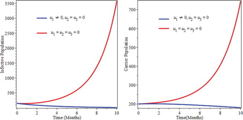
We used prevention and treatment as intervention strategy, and Figure 7 show that, the number of infective and also carriers goes down in the specified time. Therefore, this strategies is effective in eradicating the disease from the community in a specified period of time (Figure 6).

Figure 6. Simulations optimal control with prevention and treatment interventions.

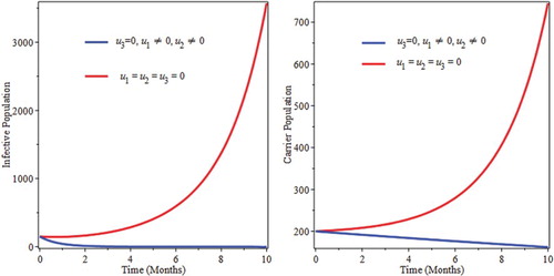
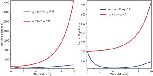
Figure 7. Simulations of optimal control with prevention and screening intervention.

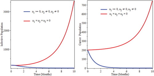
6.5. Control with prevention and screening

In this strategy we used prevention and screening. The first Figure 7 shows that the curve for optimal control is above the curve of with out control. Due to the reason that there is no treatment but individuals from carrier groups are joining infective compartment by screening and also there are a number of infected people in the compartment before prevention with out getting treatment so this situation make the curve to goes up for a time being. After some time the number of infectious goes down because due to prevention strategies, new infection is no more coming and also since there is no treatment the number of infective population start to goes down by disease causing death and natural death rates.

6.6. Control with treatment and screening

We used treatment and screening controls as intervention. From Figures 8, we observe that optimal control of the combination of treatment and screening helps to bring down the infectious as well as the carrier population which helps to eradicate the disease in the community.

Figure 8. Simulations of optimal control with treatment and screening intervention.

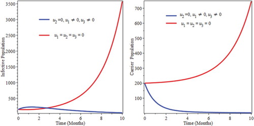
6.7. Control with prevention, treatment and screening

We implement all control the three controls interventions that helps to minimize the objective function. From Figure 9, we observe that the number of the infectious and carrier populations decrease at the specified time due to the intervention strategies. Therefore, applying this strategy helps to eradicate pneumonia disease in specified period of time (Figure 10).

Figure 9. Simulations of optimal control with Prevention, Treatment and screening interventions.

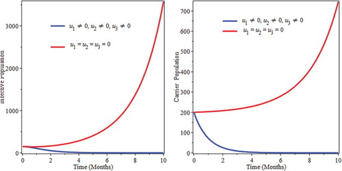
Figure 10. Backward bifurcation of the force of infection at equilibrium against the effective reproduction number $R_{\mathrm{eff}}$.

7. Cost-effectiveness analysis

Cost-effectiveness analysis used to rank the implemented strategies interims of their cost. Applying one intervention only might to be effective to eradicate the disease from the community. Therefore, we analysed strategies that used more than one intervention method. To achieve, this we used incremental cost-effectiveness ratio (ICER), stated by Baba and Makinde [1]; $``\mathsf{I}\mathsf{C}\mathsf{E}\mathsf{R}\mathsf{=}\frac{\mathsf{D}\mathsf{i}\mathsf{f}\mathsf{f}\mathsf{e}\mathsf{r}\mathsf{e}\mathsf{n}\mathsf{c}\mathsf{e}\mathsf{i}\mathsf{n}\mathsf{c}\mathsf{o}\mathsf{s}\mathsf{t}\mathsf{s}\mathsf{b}\mathsf{e}\mathsf{t}\mathsf{w}\mathsf{e}\mathsf{e}\mathsf{n}\mathsf{s}\mathsf{t}\mathsf{r}\mathsf{a}\mathsf{t}\mathsf{e}\mathsf{g}\mathsf{i}\mathsf{e}\mathsf{s}}{\mathsf{D}\mathsf{i}\mathsf{f}\mathsf{f}\mathsf{e}\mathsf{r}\mathsf{e}\mathsf{n}\mathsf{c}\mathsf{e}\mathsf{i}\mathsf{n}\mathsf{h}\mathsf{e}\mathsf{a}\mathsf{l}\mathsf{t}\mathsf{h}\mathsf{e}\mathsf{f}\mathsf{f}\mathsf{e}\mathsf{c}\mathsf{t}\mathsf{s}\mathsf{b}\mathsf{e}\mathsf{t}\mathsf{w}\mathsf{e}\mathsf{e}\mathsf{n}\mathsf{s}\mathsf{t}\mathsf{r}\mathsf{a}\mathsf{t}\mathsf{e}\mathsf{g}\mathsf{i}\mathsf{e}\mathsf{s}}\mathsf{.}{}^{″}$

In Table 3 we obtain the total number of infectious averted and total cost for the implemented strategies. The difference between the total infectious individuals without control and the total infectious individuals with control is used to obtain the total number of infectious averted. And also to find the total cost for the implemented strategies we used the cost function, which is $\frac{1}{2}{w}_1{u}_1^2,\frac{1}{2}{w}_2{u}_2^2$ and $\frac{1}{2}{w}_3{u}_3^2$ over time. We used the parameter values in Table 2 and to apply ICER technique first we ordered the intervention strategies for pairwise comparison as in Table 2 from A to D with increasing order of effectiveness.

Table 3. Number of infectious averted and total cost of each strategies.

Strategies	Description	Total infectious averted	Total cost (USD)
A	Vaccination and screening	101,417	5906.1
B	Treatment and screening	116,099	5472.7
C	Prevention and treatment	117,142	5292
D	Prevention, treatment and screening	119,465	6948.8

First, we compared the cost effectiveness of strategy A and B. $\begin{array}{rl}\mathrm{ICER}\left(\mathrm{A}\right)& =\frac{5,906.1}{101,417}=0.058,\\ \mathrm{ICER}\left(\mathrm{B}\right)& =\frac{5,472.7-5,906.1}{116,099-101,417}=-\mathrm{0.029.}\end{array}$ From ICER (A) and ICER (B), we can see that strategy B saves 0.029 than strategy A. Therefore, we exclude strategy A, because it is a bit expensive continue to compare strategy B and C. $\begin{array}{rl}\mathrm{ICER}\left(\mathrm{B}\right)& =\frac{5,472.7}{116,099}=0.047,\\ \mathrm{ICER}\left(\mathrm{C}\right)& =\frac{5,292-5,472.7}{117,142-116,099}=-\mathrm{0.0015.}\end{array}$ Similarly, from ICER (B) and ICER (C) we can see that strategy C saves 0.0015 than strategy B. Therefore, we exclude strategy B, because it is a bit expensive and finally, we compared strategy C and D. $\begin{array}{rl}\mathrm{ICER}\left(\mathrm{C}\right)& =\frac{5,292}{117,142}=0.045,\\ \mathrm{ICER}\left(\mathrm{D}\right)& =\frac{6,948.8-5,292}{119,465-117,142}=\mathrm{0.71.}\end{array}$ From ICER (C) and ICER (D) we can see that strategy C saves 0.71 than strategy D. Therefore, we exclude strategy D, because it is a bit expensive. Therefore, we conclude that strategy C the cheapest of all compared strategies, that meant it is the most cost-effective for pneumonia disease control interventions strategy's.

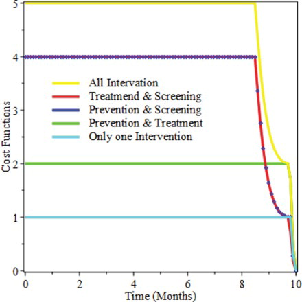
For further elaboration, Figure 11 shows that applying only one intervention costs the least interims of price but we did not consider this, due to the reason that a single intervention is not effective to eradicate the disease. And additionally we observe from the figure, applying all the three intervention at once is the most expensive of all the applied intervention strategies.

Figure 11. Cost Function of the intervention strategies for the period of 10 months.

8. Discussions and conclusions

In Section 2 we described and proposed a pneumonia model, which is deterministic in its nature and also the population is assumed to be variable in size. In Section 3 we analysed the model by obtaining the feasible region, positivity of the solution set, effective reproductive number, equilibria points and their stability. Moreover, we described the possibility of backward bifurcation in Section 3. In Section 4, sensitivity analysis and interpretation of the sensitivity index is done. In Section 5 we extended the model by applying optimal control interventions and we obtained the Hamiltonian, the adjoint variables, the characterization of the controls and the optimality system. In Section 6 we the optimality system by considering different strategies as follows:

• By applying a single control, prevention, treatment or screening.

• By applying two control, prevention and treatment.

• By applying two control, prevention and screening.

• By applying two control, treatment and screening.

• By applying all control, prevention, treatment and screening.

In Section 7 numerically we investigated cost effectiveness to determine, the least and the most expensive strategies by using ICER. From the pairwise result in this study, we conclude that, the combination of prevention and treatment is the best cost-effective strategies interims of cost as well as health benefits.

Acknowledgements

We would like to express our heartfelt appreciation to Pan African University Institute of Basic Sciences Technology and Innovation (PAUSTI) for the support and also we are grateful to the anonymous reviewers for their constructive comments, which have improved the manuscript.

Disclosure statement

No potential conflict of interest was reported by the authors.

References

- S. Baba and O.D. Makinde, Optimal control of HIV/AIDS in the workplace in the presence of careless individuals, Comput. Math. Methods Med. 2014 (2014), pp. 1--19.
- K.R. Fister, S. Lenhart, and J.S.M. Nally, Optimizing chemotherapy in an hiv model, Electron. J. Diff. Equ. 32 (1998), pp. 1–12.
- W.H. Fleming and R.W. Rishel, Deterministic and Stochastic Optimal Control, Springer, New York, 1982.
- Institute for Health Metrics and Evaluation (IHME), Pushing the pace: Progress and challenges in fighting childhood pneumonia, IHME, Seattle, WA, 2014.
- E. Joseph, Mathematical analysis of prevention and control strategies of pneumonia in adults and children, Unpublished MSc Dissertation. University of Dar es Salaam, Tanzania, 2012.
- J.P. LaSalle, The Stability of Dynamical Systems, Vol. 25, SIAM, Philadelphia, 1976.
- S. Lenhart and J.T. Workman, Optimal Control Applied to Biological Models, Mathematical and Computational Biology Series, Chapman & Hall/CRC, London, 2007.
- A. Melegaro, N.J. Gay, and G.F. Medley, Estimating the transmission parameters of pneumococcal carriage in households, Epidemiol Infect 132 (2004), pp. 433–441. doi: 10.1017/S0950268804001980
- C.A. Okaka, J.Y.T. Mugisha, A. Manyonge, and C. Ouma, Modelling the impact of misdiagnosis and treatment on the dynamics of malaria concurrent and co-infection with pneumonia, Appl. Math. Sci. (2013).
- K.O. Okosun and O.D. Makinde, Modelling the impact of drug resistance in malaria transmission and its optimal control analysis, Int. J. Phys. Sci. (2011). ISSN 19921950, doi: 10.5897/IJPS10.542.
- K.O. Okosun and O.D. Makinde, On a drug-resistant malaria model with susceptible individuals without access to basic amenities, J. Biol. Phys. 38 (2012), pp. 507–530. doi: 10.1007/s10867-012-9269-5
- K.O. Okosun and O.D. Makinde, Optimal control analysis of Malaria in the presence of nonlinear incidence rate, Appl. Comput. Math. 12(1) (2013), pp. 20–32.
- K.O. Okosun and O.D. Makinde, A co-infection model of malaria and cholera diseases with optimal control, Math. Biosci. 258 (2014), pp. 19–32. ISSN 00255564,. doi: 10.1016/j.mbs.2014.09.008
- O.P. Ongala, J. Otieno, and M. Joseph, A probabilistic estimation of the basic reproduction number: A case of control strategy of pneumonia, Sci. J. Appl. Math. Stat. 2 (2014), pp. 53–59.
- L.S. Pontryagin, V.G. Boltyanskii, R.V. Gamkrelize, and E.F. Mishchenko, The Mathematical Theory of Optimal Processes, John Wiley & Sons, New York, 1986.
- D. Ssebuliba, Mathematical modelling of the effectiveness of two training interventions on infectious diseases in Uganda, PhD thesis, Stellenbosch University, 2013.
- P. van den Driessche and J. Watmough, Reproduction numbers and sub-threshold endemic equilibria for compartmental models of disease transmission, Math. Biosci. 180 (2002), pp. 29–48. doi: 10.1016/S0025-5564(02)00108-6
- World Health Organization, Pneumonia fact sheet, November 2013. Available at http://www.who.int/mediacentre/factsheets/fs331/en/.
- World Health Organization (WHO), Pneumonia, 2015. Available at http://www.who.int/mediacentre/.