Backward bifurcation and oscillations in a nested immuno-eco-epidemiological model

ABSTRACT

This paper introduces a novel partial differential equation immuno-eco-epidemiological model of competition in which one species is affected by a disease while another can compete with it directly and by lowering the first species' immune response to the infection, a mode of competition termed stress-induced competition. When the disease is chronic, and the within-host dynamics are rapid, we reduce the partial differential equation model (PDE) to a three-dimensional ordinary differential equation (ODE) model. The ODE model exhibits backward bifurcation and sustained oscillations caused by the stress-induced competition. Furthermore, the ODE model, although not a special case of the PDE model, is useful for detecting backward bifurcation and oscillations in the PDE model. Backward bifurcation related to stress-induced competition allows the second species to persist for values of its invasion number below one. Furthermore, stress-induced competition leads to destabilization of the coexistence equilibrium and sustained oscillations in the PDE model. We suggest that complex systems such as this one may be studied by appropriately designed simple ODE models.

KEYWORDS:

• Backward bifurcation
• multi-scale models
• oscillations
• immuno-eco-epi model
• stress-induced competition
• infectious disease ecology

AMS SUBJECT CLASSIFICATION:

• 92D30

1. Introduction

Traditional epidemiology focuses on between-host transmission dynamics in single host populations [1], where hosts are categorized into discrete states (e.g. susceptible, infected, and recovered and resistant, as in classic SIR models). In recent years, epidemiological theory and practice have been enriched in several ways. One is increasing recognition that infectious disease processes occur over multiple nested scales of biological organization [4,26]. Infection of a susceptible host by a pathogen is akin to a ‘patch’ being colonized in a metapopulation [13,14], and within individual hosts there can be substantial dynamics, as the pathogen waxes and wanes in response both to its exploitation of host resources and to the host's mounting labile defences against infection. Hosts are coupled by between-host transmission, which reflects the pathogen load sustained within individual infected hosts, among many other factors. Multi-scale models that allow for closed-form computation of threshold conditions are now widespread in infectious disease research [7,25]. There is a wide variety of modelling frameworks coupling different types of dynamical models on the within-host and between-host scales [25]. We refer to these as immuno-epidemiological models. The nested framework introduced by Gilchrist and Sasaki [10] links an ODE within-host model, structured by time-since-infection, to a between-host model, structured by chronological time and time-since-infection. The linkage is achieved by expressing the between-host rates, such as transmission rate or disease-induced mortality rate as functions of the within-host dependent variables. In this respect, the linkage is unidirectional – the between-host model depends on the within-host model but not vice versa. Making the within-host model depend on the between-host variables (e.g. species abundances) has rarely been explored, and there are many challenges in making this linkage [9]. In some specific biological scenarios, linkage in this direction can be accomplished in a relatively natural way. For instance, the within-host model has been previously linked to the pathogen in the environment for some environmentally driven diseases [8,38]. When the within-host model depends on between-host variables, and vice versa, the linkage is called bidirectional. Infectious disease models with bidirectional linkage have to date been entirely ODE models; that is, both the within-host and the between-host model are ODE models with chronological time being the only independent variable.

Most frameworks that model infectious diseases in humans or in other species include only species that are infected by or transmit the pathogens [20,22]. However, most natural populations are subject to community interactions such as interspecific competition and predation [19]. Community interactions and particularly their effects on infectious diseases have been subjects of growing attention from scientists (see reviews in [12,18,27]). These community interactions can drive infectious disease processes in multiple ways [5,18]. For instance, many pathogens can be transmitted not only between individuals of a focal species, but also between these individuals and those of other species. There is now a substantial body of literature generalizing SIR and related models to multiple host species (e.g. [16,29]), and multiple parasitic agents [5,15,18,31]. Also, predators can alter infectious disease dynamics directly by changing mortality rates of infected and susceptible hosts, and indirectly by altering the recruitment rate of susceptible hosts [17]. Predation and the presence of alternative hosts can alter infectious dynamics in often complex ways (e.g. [34]). From a dynamical perspective, including ecological interactions in disease models (eco-epidemiological models) has been found to cause oscillations [37] and even chaos [21,35]. Most eco-epidemiological models are based on classical Lotka–Volterra models that include intraspecific and interspecific interference competition.

Within-host infectious disease dynamics and community interactions can themselves be intertwined in various subtle ways, because such interactions can alter internal host states. Resource availability for hosts can affect the growth potential of pathogen populations within hosts [11,32,33], as well as the ability of hosts to defend themselves against infections [30]. It is well known in the medical profession that nutrition is an important dimension of immune responses, with malnutrition magnifying the susceptibility of humans to infection [6]. This provides one causal avenue by which the community context of a host could alter within-host pathogen dynamics. A competitor that reduces the food supply of a focal host species might not only directly alter per capita growth rates, but also indirectly diminish the ability of an infected host to effectively mount an immune response to an invasive pathogen. Competitors that exert interference (e.g. via aggression or allelopathy) on a focal species can also increase stress, which is known to hamper immune responses [28]. Such competitive effects are likely to be increasing functions of the density of the competing species.

In this paper, we combine nested immuno-epidemiological models with Lotka–Volterra-type eco-epidemiological models of competition to understand the interplay between the ecological interactions and within-host pathogen dynamics. Such a union of immuno- and eco-epidemiology was first proposed in [3]. Here we go a step further and allow the within-host immune responses in a species subject to a pathogen to be affected by the population density of a competing species. We term this mode of competition ‘stress-induced’ competition. The dependence of the within-host system on a between-host variable makes the nested model bidirectionally linked, although our linking mechanism is different from the one used in environmentally driven diseases. This type of interaction and bidirectional linkage was first examined in [2]. Here we generalize the model and examine more complex properties of the model than considered in [2]. Consistent with what has been found in other bidirectionally linked models, we observe backward bifurcation occurring in the invasion number of the second species, allowing this species to persist together with susceptible and infected individuals of the first species, even when the second species' invasion number is below one. Furthermore, we find oscillations that we believe are the first example of oscillations occurring in a nested eco-epidemiological model.

This paper is structured as follows. We introduce the PDE immuno-eco-epidemiological model in the next section. In Section 3, we reduce the PDE model to a simple 3D immuno-eco-epidemiological ODE model and we investigate the system in this simple context. In Section 4, we investigate the equilibria of the full PDE model and we show that the PDE model exhibits backward bifurcation. In Section 5, we study the stability of equilibria of the PDE model and we show oscillations concurrent with coexistence of the pathogen, host, and non-host species. Section 6 summarizes our results.

2. The model

Immuno-epidemiological models link a within-host pathogen model to a between-host population-level model. These models are usually formulated for human diseases, but in the context of diseases of natural populations, where organisms experience a wide range of ecological interactions, these models are called immuno-eco-epidemiological models. In this section, we introduce an immuno-eco-epidemiological model with a new mode of competition. Typically in nested immuno-epidemiological models, the within-host model is an ODE model and does not depend on the between-host dependent variables or chronological time [25]. Here, however, we introduce a novel model with two competing species, one of which (species 1 or the host) is affected by a pathogen, while the other (species 2 or the competitor) is not. Species 2 not only directly competes with species 1, but also reduces its ability to mount an immune response to the infectious disease. This necessitates casting the within-host model in PDE form. So our model includes a mixture of distinct modalities of competitive interactions – both direct competition (as in the classic Lotka–Volterra model), and competition via suppression of immune defences in the host species.

We begin by first introducing the within-host model.

2.1. The within-host model

A model for a pathogen with density $V(\tau ,t)$ within a host that is controlled by immune cells with density $z(\tau ,t)$, where τ is the time-since-infection and t is chronological time, is given by (1) $\begin{array}{rl}{V}_t(\tau ,t)+V_{\tau }(\tau ,t)& =r_{v}V(\tau ,t)(1-qV(\tau ,t\left)\right)-aV(\tau ,t)z(\tau ,t),\\ z_t(\tau ,t)+z_{\tau }(\tau ,t)& =\frac{b_{0}V(\tau ,t)z(\tau ,t)}{\left(p{N}_2\right(t)+D)(1+b_{2}V)}-\mu z(\tau ,t).\end{array}$(1) The system has the following initial and boundary conditions: (2) $\begin{array}{rl}V(t,0)& =V_0,\\ V(0,\tau )& =\phi \left(\tau \right),\\ z(t,0)& =z_0,\\ z(0,\tau )& =\psi \left(\tau \right),\end{array}$(2) where $V_0>0$ is the pathogen density and $z_0>0$ is the immune cell density at the time of infection. Normally, $\phi \left(\tau \right)$ and $\psi \left(\tau \right)$ would be given non-negative functions; however, for this system, they are defined as follows: $\phi \left(\tau \right)=\hat{V}\left(\tau \right)$ and $\psi \left(\tau \right)=\hat{z}\left(\tau \right)$, where $\hat{V}$ and $\hat{z}$ are solutions of the following ODEs: (3) $\begin{array}{rl}{V}^{\prime }\left(\tau \right)& =r_{v}V\left(\tau \right)(1-qV(\tau \left)\right)-aV\left(\tau \right)z\left(\tau \right),\\ z^{\prime }\left(\tau \right)& =\frac{b_{0}V\left(\tau \right)z\left(\tau \right)}{\left(p{N}_2\right(0)+D)(1+b_{2}V)}-\mu z\left(\tau \right),\end{array}$(3) with $V\left(0\right)=V_0$ and $z\left(0\right)=z_0$. These equations have no effect unless there are hosts that become infected at t<0 and are still infected at t=0. If so, their internal dynamics are assumed to be those resulting from $N_2$ being fixed at its initial value (t=0) (otherwise, we would need $N_2$ for t<0).

In this system, in the absence of immune cells, the pathogen will grow logistically; $r_v$ is the intrinsic growth rate of the pathogen and q is the reciprocal of its carrying capacity, a is the attack rate of immune cells, and μ is the death rate of immune cells. The first term of the second equation in Equation (1(1) $\begin{array}{rl}{V}_t(\tau ,t)+V_{\tau }(\tau ,t)& =r_{v}V(\tau ,t)(1-qV(\tau ,t\left)\right)-aV(\tau ,t)z(\tau ,t),\\ z_t(\tau ,t)+z_{\tau }(\tau ,t)& =\frac{b_{0}V(\tau ,t)z(\tau ,t)}{\left(p{N}_2\right(t)+D)(1+b_{2}V)}-\mu z(\tau ,t).\end{array}$(1) ) is the immune cell activation rate, which saturates with increasing V, with $b_2$ being the reciprocal of the half-saturation value of V. In the population model (detailed below), there are two competing species; the pathogen affects species 1, and its maximum immune activation rate $b_0/D$ can be reduced by increasing the density of species 2, which is $N_2$. Parameter p is set to 1 to include the effect of $N_2$ on the immune response of species 1 or set to 0 to exclude this effect. The parameters and variables of the within-host model are summarized in Table 1.

Table 1. Summary of parameters and variables in model (1(1) $\begin{array}{rl}{V}_t(\tau ,t)+V_{\tau }(\tau ,t)& =r_{v}V(\tau ,t)(1-qV(\tau ,t\left)\right)-aV(\tau ,t)z(\tau ,t),\\ z_t(\tau ,t)+z_{\tau }(\tau ,t)& =\frac{b_{0}V(\tau ,t)z(\tau ,t)}{\left(p{N}_2\right(t)+D)(1+b_{2}V)}-\mu z(\tau ,t).\end{array}$(1) ).

Parameter/variable	Meaning
t	Chronological time
τ	Time-since-infection
$V(\tau ,t)$	Pathogen density
$z(\tau ,t)$	Immune cell density
$r_v$	Intrinsic growth rate of pathogen
$K_v$	Carrying capacity of the pathogen
q	$1/K_v$
a	Attack rate of immune cells
μ	Death rate of immune cells
$b_2$	Reciprocal of the half-saturation level of V
$b_0/D$	Maximum activation rate of the immune response
$N_2\left(t\right)$	Population numbers of species 2
p	Controls whether the impact of species 2 slows
	species 1's immune response

This within-host model is a PDE extension of the within-host model used in [2] if $q=1/K_v$ and $b_2=0$. To develop a simple ODE model for the within-host system, the approach in [2] was to assume that the impact of $N_2$ does not change during the entire within-host infection and it is fixed at present time. We dispose of this assumption here and use a more realistic model where the time-since-infection τ and chronological time t progress simultaneously.

We assume $r_v>0$, since if this is not true the pathogen can never increase, and $b_0>0$, as otherwise the immune cells can never increase. Also, the immune system has no effect on the pathogen if a=0, so we assume a>0. Parameter $b_2$ is non-negative; if positive, immune activation saturates at high V. The other parameters ($q,\mu$ and D) can be either 0 or positive (but D cannot be 0 if $N_2$ is 0 or if p is 0). For chronic infection, μ must be greater than 0, but this model with $\mu =0$ can be used for acute infection with permanent immunity.

2.2. The between-host model

There are many ways to splice epidemiological models with species interaction models. As a step towards greater realism, we will explore models in which the within-host model is embedded in a classic two-species Lotka–Volterra competition model with the pathogen specialized to one species [see Equations (4(4) $\begin{array}{rl}{S}^{\prime }& =r_1\left(1-\frac{N_1+{\alpha }_{12}{N}_2}{K_1}\right)N_1-S\left(t\right){\int }_0^{\mathrm{\infty }}\beta \left(\tau \right)i(\tau ,t)\mathrm{d}\tau -m_{1}S\left(t\right),\\ i_{\tau }(\tau ,t)+i_t(\tau ,t)& =-(m_1+\alpha (\tau )+\gamma (\tau \left)\right)i(\tau ,t),\\ i(0,t)& =S\left(t\right){\int }_0^{\mathrm{\infty }}\beta \left(\tau \right)i(\tau ,t)\mathrm{d}\tau ,\\ R^{\prime }& ={\int }_0^{\mathrm{\infty }}\gamma \left(\tau \right)i(\tau ,t)\mathrm{d}\tau -m_{1}R,\\ N_2^{\prime }\left(t\right)& =r_2\left(1-\frac{N_2+{\alpha }_{21}{N}_1}{K_2}\right)N_2-m_2{N}_2.\end{array}$(4) )]. We will address several questions. How does pathogen reproduction rate alter prior coexistence/dominance relationships between the species? If competition is expressed via weakening of the immune response (as above), how does this alter equilibrial prevalence, conditions for disease spread, and potentially unstable dynamics? Our goal is to study the interplay of within-host pathogen and immune dynamics and basic ecological interactions. The species that can be infected, species 1, is structured by time-since-infection and its immune status is tracked. The resulting novel immuno-eco-epidemiological model can be used to study how competition influences the interaction of the pathogen with the immune system and how this within-host dynamic interaction in turn affects the population dynamics of the two species.

To introduce the model (see Table 2 for parameters and variables), let $N_i\left(t\right)$ be the total number of individuals in species i (i=1,2) at time t. Species 1 can be infected by a pathogen and can contain susceptible hosts $S\left(t\right)$, recovered hosts $R\left(t\right)$, and infected hosts structured by time-since-infection τ; $i(\tau ,t)$ is the density of infected hosts at time t that were infected τ time units previously. The total population of species 1 is $N_1\left(t\right)=S\left(t\right)+{\int }_0^{\mathrm{\infty }}i(\tau ,t)\mathrm{d}\tau +R\left(t\right).$ Changes in these variables are described by the equations (4) $\begin{array}{rl}{S}^{\prime }& =r_1\left(1-\frac{N_1+{\alpha }_{12}{N}_2}{K_1}\right)N_1-S\left(t\right){\int }_0^{\mathrm{\infty }}\beta \left(\tau \right)i(\tau ,t)\mathrm{d}\tau -m_{1}S\left(t\right),\\ i_{\tau }(\tau ,t)+i_t(\tau ,t)& =-(m_1+\alpha (\tau )+\gamma (\tau \left)\right)i(\tau ,t),\\ i(0,t)& =S\left(t\right){\int }_0^{\mathrm{\infty }}\beta \left(\tau \right)i(\tau ,t)\mathrm{d}\tau ,\\ R^{\prime }& ={\int }_0^{\mathrm{\infty }}\gamma \left(\tau \right)i(\tau ,t)\mathrm{d}\tau -m_{1}R,\\ N_2^{\prime }\left(t\right)& =r_2\left(1-\frac{N_2+{\alpha }_{21}{N}_1}{K_2}\right)N_2-m_2{N}_2.\end{array}$(4) This model has initial conditions $S\left(0\right)=S_0$, $i(\tau ,0)=\varphi \left(\tau \right)$, $R\left(0\right)=R_0$, $N_2\left(0\right)=N_2^0$. We assume that $S_0$ and $N_2^0$ are positive and $\varphi \left(\tau \right),R_0\ge 0$. Further, we assume that all hosts reproduce and all offspring are born susceptible (i.e. no vertical transmission). The per capita growth rate of each species is described by a logistic function where $r_i$ is the intrinsic per capita growth rate and $K_i$ the density of species i at which the growth rate is 0 in the absence of the other species. There is a component of density-independent intrinsic per capita death rates, represented as a constant, $m_i$ ($r_i,K_i,m_i>0$). Each species can reduce the growth rate of the other, with ${\alpha }_{ij}$ (both non-negative) giving the reduction of the growth rate of species i due to an individual of species j relative to the reduction caused by an individual of species i (so ${\alpha }_{11}={\alpha }_{22}=1$). The rate of infection of each susceptible host (per infected host) is $\beta \left(\tau \right)$, and the disease-induced mortality rate is $\alpha \left(\tau \right)$, both of which are increasing functions of V (and could also depend on z). We use the functions in Table 3.

Table 2. Summary of parameters and variables in model (4(4) $\begin{array}{rl}{S}^{\prime }& =r_1\left(1-\frac{N_1+{\alpha }_{12}{N}_2}{K_1}\right)N_1-S\left(t\right){\int }_0^{\mathrm{\infty }}\beta \left(\tau \right)i(\tau ,t)\mathrm{d}\tau -m_{1}S\left(t\right),\\ i_{\tau }(\tau ,t)+i_t(\tau ,t)& =-(m_1+\alpha (\tau )+\gamma (\tau \left)\right)i(\tau ,t),\\ i(0,t)& =S\left(t\right){\int }_0^{\mathrm{\infty }}\beta \left(\tau \right)i(\tau ,t)\mathrm{d}\tau ,\\ R^{\prime }& ={\int }_0^{\mathrm{\infty }}\gamma \left(\tau \right)i(\tau ,t)\mathrm{d}\tau -m_{1}R,\\ N_2^{\prime }\left(t\right)& =r_2\left(1-\frac{N_2+{\alpha }_{21}{N}_1}{K_2}\right)N_2-m_2{N}_2.\end{array}$(4) ).

Parameter/variable	Meaning
S	Number of susceptibles of species 1
$i(\tau ,t)$	Density of infectives in species 1
R	Number of recovereds in species 1
$N_j\left(t\right)$	Population size of species j
$r_i$	Intrinsic growth rate of species i
$K_i$	Carrying capacity of species i
$m_i$	Intrinsic death rate of species i
$\beta \left(\tau \right)$	Transmission rate
$\alpha \left(\tau \right)$	Disease-induced death rate
$\gamma \left(\tau \right)$	Recovery rate
${\alpha }_{ij}$	Competition coefficient giving effect of species j
	on species i

Table 3. Summary of linking functions.

Version	$\beta \left(\tau \right)$	$\alpha \left(\tau \right)$	Remarks
1	$\beta \left(t\right)=c{V}^{\ast }\left(t\right)$	$\alpha \left(t\right)=\eta V^{\ast }\left(t\right)$	Used in Section 3
2	$\beta \left(\tau \right)={\displaystyle \frac{{\beta }_{0}V\left(\tau \right)}{V\left(\tau \right)+B}}$	$\alpha \left(\tau \right)=\eta V\left(\tau \right)$	Used in Figure 7
3	$\beta \left(\tau \right)={\beta }_{0}V\left(\tau \right)$	$\alpha \left(\tau \right)=\eta V\left(\tau \right)$	Used in Figure 6

For the model with recovery, $\gamma \left(\tau \right)$ is the rate at which infected hosts recover, which should be an increasing function of z and a decreasing function of V, such as assumed as in [36]: $\gamma \left(\tau \right)=\frac{\kappa z}{V+{ϵ}_0},$ where ${ϵ}_0$ is a small constant. The transmission rate $\beta \left(\tau \right)$ and the disease-induced death rate $\alpha \left(\tau \right)$ and recovery rate $\gamma \left(\tau \right)$ potentially depend implicitly on $N_2$ and on t. Although we will be suppressing this dependence below, it should always be kept in mind as they provide mechanistic pathways by which a competing species could alter infectious disease dynamics in a focal host species.

In Section 3, we assume that the within-host dynamics are fast enough that V and z follow their within-host equilibria, and β and α are functions only of t. For equilibria of the between-host system, such as those in Figure 6, there is no dependence on t so β and α are functions of τ only. For the chronic infection case (next section), $\mu >0$ and infected hosts do not recover, so $\kappa =0$ (also $R=0$). If $\mu =0$, there is recovery, so $\kappa >0$.

3. Chronic infection with fast internal dynamics

To understand better the impact of species 2 on the immune system of species 1, we consider model (1(1) $\begin{array}{rl}{V}_t(\tau ,t)+V_{\tau }(\tau ,t)& =r_{v}V(\tau ,t)(1-qV(\tau ,t\left)\right)-aV(\tau ,t)z(\tau ,t),\\ z_t(\tau ,t)+z_{\tau }(\tau ,t)& =\frac{b_{0}V(\tau ,t)z(\tau ,t)}{\left(p{N}_2\right(t)+D)(1+b_{2}V)}-\mu z(\tau ,t).\end{array}$(1) )–(4(4) $\begin{array}{rl}{S}^{\prime }& =r_1\left(1-\frac{N_1+{\alpha }_{12}{N}_2}{K_1}\right)N_1-S\left(t\right){\int }_0^{\mathrm{\infty }}\beta \left(\tau \right)i(\tau ,t)\mathrm{d}\tau -m_{1}S\left(t\right),\\ i_{\tau }(\tau ,t)+i_t(\tau ,t)& =-(m_1+\alpha (\tau )+\gamma (\tau \left)\right)i(\tau ,t),\\ i(0,t)& =S\left(t\right){\int }_0^{\mathrm{\infty }}\beta \left(\tau \right)i(\tau ,t)\mathrm{d}\tau ,\\ R^{\prime }& ={\int }_0^{\mathrm{\infty }}\gamma \left(\tau \right)i(\tau ,t)\mathrm{d}\tau -m_{1}R,\\ N_2^{\prime }\left(t\right)& =r_2\left(1-\frac{N_2+{\alpha }_{21}{N}_1}{K_2}\right)N_2-m_2{N}_2.\end{array}$(4) ) in the case for which there is no recovery and the disease is chronic (which requires $\mu >0$, in which case the within-host system goes to a stable equilibrium with the pathogen present for constant $N_2$). We assume that the dynamics of the pathogen with the immune system are sufficiently rapid so that they can be assumed to always be at their equilibrium. To simplify matters and gain more insight, we will also assume a linear dependence of the transmission rate and disease-induced mortality on pathogen density: $\beta \left(t\right)=c{V}^{\ast }\left(t\right),\alpha \left(t\right)=\eta V^{\ast }\left(t\right),$ where $V^{\ast }\left(t\right)$ is the equilibrium pathogen density if $N_2$ were fixed at $N_2\left(t\right)$. Note that this is the within-host equilibrium. The between-host model need not be at equilibrium, and $N_2\left(t\right)$ can vary with time, in which case $V^{\ast }\left(t\right)$ and therefore β and α vary with time. $V^{\ast }\left(t\right)$ approximates the solution to Equation (1(1) $\begin{array}{rl}{V}_t(\tau ,t)+V_{\tau }(\tau ,t)& =r_{v}V(\tau ,t)(1-qV(\tau ,t\left)\right)-aV(\tau ,t)z(\tau ,t),\\ z_t(\tau ,t)+z_{\tau }(\tau ,t)& =\frac{b_{0}V(\tau ,t)z(\tau ,t)}{\left(p{N}_2\right(t)+D)(1+b_{2}V)}-\mu z(\tau ,t).\end{array}$(1) ) if $N_2\left(t\right)$ changes slowly relative to the time it takes for the equations to reach the within-host equilibrium (so we can neglect the derivatives with respect to t). Furthermore, we assume $b_2=0$. In this case $V^{\ast }\left(t\right)=\mu \left(N_2\right(t)+D)/b_0$ and $\beta \left(t\right)=\beta \left(N_2\right)$, $\alpha \left(t\right)=\alpha \left(N_2\right)$ where $\beta \left(N_2\right)=\frac{c\mu (p{N}_2+D)}{b_0},\alpha \left(N_2\right)=\frac{\eta \mu (p{N}_2+D)}{b_0}.$

Then system (4(4) $\begin{array}{rl}{S}^{\prime }& =r_1\left(1-\frac{N_1+{\alpha }_{12}{N}_2}{K_1}\right)N_1-S\left(t\right){\int }_0^{\mathrm{\infty }}\beta \left(\tau \right)i(\tau ,t)\mathrm{d}\tau -m_{1}S\left(t\right),\\ i_{\tau }(\tau ,t)+i_t(\tau ,t)& =-(m_1+\alpha (\tau )+\gamma (\tau \left)\right)i(\tau ,t),\\ i(0,t)& =S\left(t\right){\int }_0^{\mathrm{\infty }}\beta \left(\tau \right)i(\tau ,t)\mathrm{d}\tau ,\\ R^{\prime }& ={\int }_0^{\mathrm{\infty }}\gamma \left(\tau \right)i(\tau ,t)\mathrm{d}\tau -m_{1}R,\\ N_2^{\prime }\left(t\right)& =r_2\left(1-\frac{N_2+{\alpha }_{21}{N}_1}{K_2}\right)N_2-m_2{N}_2.\end{array}$(4) ) becomes the following ODE model: (5) $\begin{array}{rl}{S}^{\prime }& =r_1\left(1-\frac{N_1+{\alpha }_{12}{N}_2}{K_1}\right)N_1-\beta \left(N_2\right)SI-m_{1}S,\\ I^{\prime }& =\beta \left(N_2\right)SI-(m_1+\alpha (N_2\left)\right)I,\\ N_2^{\prime }& =r_2\left(1-\frac{N_2+{\alpha }_{21}{N}_1}{K_2}\right)N_2-m_2{N}_2.\end{array}$(5)

Model (5(5) $\begin{array}{rl}{S}^{\prime }& =r_1\left(1-\frac{N_1+{\alpha }_{12}{N}_2}{K_1}\right)N_1-\beta \left(N_2\right)SI-m_{1}S,\\ I^{\prime }& =\beta \left(N_2\right)SI-(m_1+\alpha (N_2\left)\right)I,\\ N_2^{\prime }& =r_2\left(1-\frac{N_2+{\alpha }_{21}{N}_1}{K_2}\right)N_2-m_2{N}_2.\end{array}$(5) ) is a new type of eco-epidemiological model in which the competitor (species 2) affects the host (species 1) not only through competition for resources but also by affecting the disease transmission and disease-induced death rates, both of which increase with $N_2$ as shown above. Setting p=0 eliminates this effect, and makes Equation (5(5) $\begin{array}{rl}{S}^{\prime }& =r_1\left(1-\frac{N_1+{\alpha }_{12}{N}_2}{K_1}\right)N_1-\beta \left(N_2\right)SI-m_{1}S,\\ I^{\prime }& =\beta \left(N_2\right)SI-(m_1+\alpha (N_2\left)\right)I,\\ N_2^{\prime }& =r_2\left(1-\frac{N_2+{\alpha }_{21}{N}_1}{K_2}\right)N_2-m_2{N}_2.\end{array}$(5) ) a classical eco-epidemiological model. Therefore, comparing Equation (5(5) $\begin{array}{rl}{S}^{\prime }& =r_1\left(1-\frac{N_1+{\alpha }_{12}{N}_2}{K_1}\right)N_1-\beta \left(N_2\right)SI-m_{1}S,\\ I^{\prime }& =\beta \left(N_2\right)SI-(m_1+\alpha (N_2\left)\right)I,\\ N_2^{\prime }& =r_2\left(1-\frac{N_2+{\alpha }_{21}{N}_1}{K_2}\right)N_2-m_2{N}_2.\end{array}$(5) ) with p=0 and with p=1 allows us to compare this novel model to the corresponding classical model. To simplify the notation, we can define ${\beta }_0=c\mu /b_0$ and ${\alpha }_0=\eta \mu /b_0$. We note that species 2 both facilitates pathogen spread in species 1, via boosting β, and hampers it, by increasing α.

3.1. Equilibria of model (5(5) $\begin{array}{rl}{S}^{\prime }& =r_1\left(1-\frac{N_1+{\alpha }_{12}{N}_2}{K_1}\right)N_1-\beta \left(N_2\right)SI-m_{1}S,\\ I^{\prime }& =\beta \left(N_2\right)SI-(m_1+\alpha (N_2\left)\right)I,\\ N_2^{\prime }& =r_2\left(1-\frac{N_2+{\alpha }_{21}{N}_1}{K_2}\right)N_2-m_2{N}_2.\end{array}$(5) )

System (5(5) $\begin{array}{rl}{S}^{\prime }& =r_1\left(1-\frac{N_1+{\alpha }_{12}{N}_2}{K_1}\right)N_1-\beta \left(N_2\right)SI-m_{1}S,\\ I^{\prime }& =\beta \left(N_2\right)SI-(m_1+\alpha (N_2\left)\right)I,\\ N_2^{\prime }& =r_2\left(1-\frac{N_2+{\alpha }_{21}{N}_1}{K_2}\right)N_2-m_2{N}_2.\end{array}$(5) ) has the extinction equilibrium ${\mathcal{E}}_0=(0,0,0)$, which always exists. Next, we have the species-2-only equilibrium ${\mathcal{E}}_2=(0,0,{\hat{N}}_2)$, where ${\hat{N}}_2=K_2(1-m_2/r_2)$, which exists only if $r_2>m_2$. Symmetrically, system (5(5) $\begin{array}{rl}{S}^{\prime }& =r_1\left(1-\frac{N_1+{\alpha }_{12}{N}_2}{K_1}\right)N_1-\beta \left(N_2\right)SI-m_{1}S,\\ I^{\prime }& =\beta \left(N_2\right)SI-(m_1+\alpha (N_2\left)\right)I,\\ N_2^{\prime }& =r_2\left(1-\frac{N_2+{\alpha }_{21}{N}_1}{K_2}\right)N_2-m_2{N}_2.\end{array}$(5) ) has the no-disease, species-1-only equilibrium ${\mathcal{E}}_1=({\hat{N}}_1,0,0)$, where ${\hat{N}}_1=K_1(1-m_1/r_1)$. This equilibrium exists only if $r_1>m_1$. Define the reproduction numbers of species i in the absence of disease as ${\mathcal{R}}_i=\frac{r_i}{m_i}.$

Proposition 3.1

Equilibrium ${\mathcal{E}}_1$ exists if and only if ${\mathcal{R}}_1>1$. Equilibrium ${\mathcal{E}}_2$ exists if and only if ${\mathcal{R}}_2>1$.

Assume ${\mathcal{R}}_1>1$ and ${\mathcal{R}}_2>1$. Then the system has another disease-free equilibrium: the no-disease coexistence equilibrium ${\mathcal{E}}_{12}=({\overline{N}}_1,0,{\overline{N}}_2),$ where (6) $\begin{array}{rl}{\overline{N}}_1& =\frac{K_1\left(1-{\displaystyle \frac{m_1}{r_1}}\right)-{\alpha }_{12}{K}_2\left(1-{\displaystyle \frac{m_2}{r_2}}\right)}{1-{\alpha }_{12}{\alpha }_{21}},\\ {\overline{N}}_2& =\frac{K_2\left(1-{\displaystyle \frac{m_2}{r_2}}\right)-{\alpha }_{21}{K}_1\left(1-{\displaystyle \frac{m_1}{r_1}}\right)}{1-{\alpha }_{12}{\alpha }_{21}}.\end{array}$(6)

Proposition 3.2

Assume ${\mathcal{R}}_1>1$ and ${\mathcal{R}}_2>1$. Equilibrium ${\mathcal{E}}_{12}$ exists if and only if one of the following two sets of inequalities are satisfied: (7) $\begin{array}{r}{K}_1\left(1-\frac{m_1}{r_1}\right)-{\alpha }_{12}{K}_2\left(1-\frac{m_2}{r_2}\right)>0,\\ K_2\left(1-\frac{m_2}{r_2}\right)-{\alpha }_{21}{K}_1\left(1-\frac{m_1}{r_1}\right)>0\end{array}$(7) or (8) $\begin{array}{r}{K}_1\left(1-\frac{m_1}{r_1}\right)-{\alpha }_{12}{K}_2\left(1-\frac{m_2}{r_2}\right)<0,\\ K_2\left(1-\frac{m_2}{r_2}\right)-{\alpha }_{21}{K}_1\left(1-\frac{m_1}{r_1}\right)<0.\end{array}$(8)

Note that the first set of inequalities implies $1-{\alpha }_{12}{\alpha }_{21}>0$. Similarly, the second set of inequalities implies $1-{\alpha }_{12}{\alpha }_{21}<0$. In the former case, in the absence of the infectious disease, given that coexistence is feasible, the equilibrium is locally stable (the coexistence scenario of classical Lotka–Volterra competition). In the latter case, the equilibrium (if feasible) is unstable, corresponding to a priority effect in the classical Lotka–Volterra competition. Another equilibrium, ${\mathcal{E}}^{\ast }$, has species 1 with the disease but without species 2. To show the existence of equilibrium ${\mathcal{E}}^{\ast }$, we define the reproduction number of the disease in the absence of the competitor: ${\mathcal{R}}_0=\frac{\beta \left(0\right){\hat{N}}_1}{m_1+\alpha \left(0\right)}.$

Proposition 3.3

Assume ${\mathcal{R}}_1>1$ and ${\mathcal{R}}_0>1$. Then the system (5(5) $\begin{array}{rl}{S}^{\prime }& =r_1\left(1-\frac{N_1+{\alpha }_{12}{N}_2}{K_1}\right)N_1-\beta \left(N_2\right)SI-m_{1}S,\\ I^{\prime }& =\beta \left(N_2\right)SI-(m_1+\alpha (N_2\left)\right)I,\\ N_2^{\prime }& =r_2\left(1-\frac{N_2+{\alpha }_{21}{N}_1}{K_2}\right)N_2-m_2{N}_2.\end{array}$(5) ) has a unique equilibrium ${\mathcal{E}}^{\ast }=(S^{\ast },I^{\ast },0)$.

This is not hard to demonstrate. We set $N_2^{\ast }=0$ in the equilibrial equations and solve for S and I. $S^{\ast }=\frac{m_1+\alpha \left(0\right)}{\beta \left(0\right)},$ $I^{\ast }=N_1^{\ast }-S^{\ast }$ and $N_1^{\ast }$ is the unique positive solution of the equation: $r_1\left(1-\frac{N_1}{K_1}\right)N_1-m_{1}S=(m_1+\alpha (0\left)\right)(N_1-S).$ This equation rewritten as a quadratic equation in $N_1$ has a positive leading term and a negative constant term, and therefore, a unique positive solution. To see that $S^{\ast }<N_1^{\ast }$ so that $I^{\ast }>0,$ we notice that the condition ${\mathcal{R}}_0>1$ implies $S^{\ast }<{\hat{N}}_1$. Using this inequality, it is not hard to see that the solution of the above equation occurs in the interval $(S^{\ast },K_1)$. Finally, there is the coexistence equilibrium ${\mathcal{E}}^{\ast \ast }$. In principle, there are two ways in which coexistence equilibria can be reached in this model. One is that the pathogen may invade the state with coexistence of the two species without disease (if the equilibrium ${\mathcal{E}}_{12}$ exists). This process requires that ${\mathcal{R}}_{00}>1$, where ${\mathcal{R}}_{00}=\frac{\beta \left({\overline{N}}_2\right){\overline{N}}_1}{m_1+\alpha \left({\overline{N}}_2\right)}$ is the reproduction number of the disease in the presence of the competitor. The second way a coexistence equilibrium may be reached is by species 2 invading species 1 with disease equilibrium ${\mathcal{E}}^{\ast }$. This is regulated by the species 2 invasion number ${\hat{\mathcal{R}}}_2$, defined as: ${\hat{\mathcal{R}}}_2=\frac{r_2}{m_2+\frac{r_2{\alpha }_{21}{N}_1^{\ast }}{K_2}}.$ For the coexistence equilibrium, we use the explicit dependence of $\alpha \left(N_2\right)$ and $\beta \left(N_2\right)$ on $N_2$.

Proposition 3.4

Assume ${\mathcal{R}}_i>1$ for i=1,2. The coexistence equilibrium ${\mathcal{E}}^{\ast \ast }=(S^{\ast \ast },I^{\ast \ast },N_2^{\ast \ast })$ of system (5(5) $\begin{array}{rl}{S}^{\prime }& =r_1\left(1-\frac{N_1+{\alpha }_{12}{N}_2}{K_1}\right)N_1-\beta \left(N_2\right)SI-m_{1}S,\\ I^{\prime }& =\beta \left(N_2\right)SI-(m_1+\alpha (N_2\left)\right)I,\\ N_2^{\prime }& =r_2\left(1-\frac{N_2+{\alpha }_{21}{N}_1}{K_2}\right)N_2-m_2{N}_2.\end{array}$(5) ) exists if ${\mathcal{R}}_{00}>1$ or ${\hat{\mathcal{R}}}_2>1$ and it is unique if p=0 and $1-{\alpha }_{12}{\alpha }_{21}>0$.

Proof.

For system (5(5) $\begin{array}{rl}{S}^{\prime }& =r_1\left(1-\frac{N_1+{\alpha }_{12}{N}_2}{K_1}\right)N_1-\beta \left(N_2\right)SI-m_{1}S,\\ I^{\prime }& =\beta \left(N_2\right)SI-(m_1+\alpha (N_2\left)\right)I,\\ N_2^{\prime }& =r_2\left(1-\frac{N_2+{\alpha }_{21}{N}_1}{K_2}\right)N_2-m_2{N}_2.\end{array}$(5) ) at the coexistence equilibrium, we can solve the second equation for $S^{\ast \ast }$ in terms of $N_2$ (9) $S^{\ast \ast }=\frac{m_1+{\alpha }_0(p{N}_2+D)}{{\beta }_0(p{N}_2+D)}.$(9) Note that the number of susceptible hosts at equilibrium is a decreasing function of $N_2$ for p>0. If p=0 species 2 does not affect species 1's immune system, and the number of susceptibles will be unaffected by species 2.

From the last equation of (5(5) $\begin{array}{rl}{S}^{\prime }& =r_1\left(1-\frac{N_1+{\alpha }_{12}{N}_2}{K_1}\right)N_1-\beta \left(N_2\right)SI-m_{1}S,\\ I^{\prime }& =\beta \left(N_2\right)SI-(m_1+\alpha (N_2\left)\right)I,\\ N_2^{\prime }& =r_2\left(1-\frac{N_2+{\alpha }_{21}{N}_1}{K_2}\right)N_2-m_2{N}_2.\end{array}$(5) ), we express $N_1^{\ast \ast }$ in terms of $N_2$: (10) $N_1^{\ast \ast }=\frac{1}{{\alpha }_{21}}\left(K_2\left(1-\frac{m_2}{r_2}\right)-N_2\right).$(10) This gives $I^{\ast \ast }=N_1^{\ast \ast }-S^{\ast \ast }=\frac{1}{{\alpha }_{21}}\left(K_2\left(1-\frac{m_2}{r_2}\right)-N_2\right)-\frac{m_1+{\alpha }_0(p{N}_2+D)}{{\beta }_0(p{N}_2+D)}.$ $I^{\ast \ast }$ can be monotonically decreasing or have a hump-shaped form where it is increasing for small $N_2$ and decreasing for large $N_2$ if p=1. In contrast, if p=0, $I^{\ast \ast }$ is a strictly decreasing function of species 2 numbers. Thus, species 2, through its impact on species 1's immune response, can indirectly increase the prevalence of the disease in species 1. With p=0, the only species interaction is competition, so species 2 tends to decrease the numbers of species 1. If this decrease is enough, it could prevent the pathogen from persisting. But if the infectious disease can persist, the number of infected at equilibrium is reduced since the number of susceptibles is fixed by the second equation in Equation (5(5) $\begin{array}{rl}{S}^{\prime }& =r_1\left(1-\frac{N_1+{\alpha }_{12}{N}_2}{K_1}\right)N_1-\beta \left(N_2\right)SI-m_{1}S,\\ I^{\prime }& =\beta \left(N_2\right)SI-(m_1+\alpha (N_2\left)\right)I,\\ N_2^{\prime }& =r_2\left(1-\frac{N_2+{\alpha }_{21}{N}_1}{K_2}\right)N_2-m_2{N}_2.\end{array}$(5) ). If p=1, in contrast, there is the additional interaction through the effect on species 1's immune system, which causes β and α to increase. This can tend to make it easier for the infection to persist and also to increase the number of infected. So with p=1, there are contrasting effects of $N_2$, and the net effect can be in either direction. Increasing $N_2$ increases $I^{\ast \ast }$ at low $N_2$ if $m_{1}p/\left({\beta }_0{D}^2\right)>1/{\alpha }_{21}$; the left side measures the effect of $N_2$ due to the effect on the immune system while the right measures the direct competitive effect, and if the inequality is true the former effect outweighs the latter.

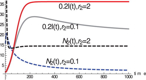
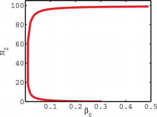
We illustrate this situation in the dynamical behaviour of the model. Figure 1 shows that increasing species 2's reproductive rate $r_2$ causes an increase in species 2 equilibrial numbers and can increase the prevalence of the disease $I\left(t\right)$ in species 1. In this case, it furthermore increases the proportion of infected of species 1 $I\left(t\right)/N_1\left(t\right)$. This effect in part is due to the impact species 2 has on the immune response of species 1. In most eco-epidemiological models, typically the negative ecological interaction decreases the prevalence in the focal species (as it does in the model above with p=0); however, there are exceptions where increase may occur [17]. To see the existence and the multiplicity of the coexistence equilibria, we add the first two equations in Equation (5(5) $\begin{array}{rl}{S}^{\prime }& =r_1\left(1-\frac{N_1+{\alpha }_{12}{N}_2}{K_1}\right)N_1-\beta \left(N_2\right)SI-m_{1}S,\\ I^{\prime }& =\beta \left(N_2\right)SI-(m_1+\alpha (N_2\left)\right)I,\\ N_2^{\prime }& =r_2\left(1-\frac{N_2+{\alpha }_{21}{N}_1}{K_2}\right)N_2-m_2{N}_2.\end{array}$(5) ) at equilibrium, and replace $N_1^{\ast \ast }$ and $I^{\ast \ast }$ with the expressions above. Thus, we arrive at the following equation for $N_2$: (11) $\begin{array}{rl}& \frac{r_1}{({\alpha }_{21}{)}^2{K}_1}\left[K_2\left(1-\frac{m_2}{r_2}\right)-N_2\right]\left[{\alpha }_{21}{K}_1\left(1-\frac{m_1}{r_1}\right)-K_2\left(1-\frac{m_2}{r_2}\right)+(1-{\alpha }_{12}{\alpha }_{21})N_2\right]\\ & ={\alpha }_0(p{N}_2+D)\left[\frac{1}{{\alpha }_{21}}\left[K_2\left(1-\frac{m_2}{r_2}\right)-N_2\right]-\frac{m_1+{\alpha }_0(p{N}_2+D)}{{\beta }_0(p{N}_2+D)}\right].\end{array}$(11) This equation is a quadratic equation in $N_2$ so it has at most two positive solutions.

Figure 1. For $r_2=2$ the equilibrial numbers of species 2 $N_2\left(t\right)$ are higher than the equilibrium number of species 2 for $r_2=0.1$. Moreover, the equilibrial prevalence $I\left(t\right)$ for species 1 is also higher. $r_1=0.5$, c=0.01, $\mu =1$, p=1, D=5, $m_1=m_2=0.01$, ${\alpha }_{12}=0.5$, ${\alpha }_{21}=0.3$, $K_1=300$, $b_0=1000$, $\eta =0.5$, $K_2=100$.

Case 1:	Equilibrium ${\mathcal{E}}_{12}$ exists, ${\alpha }_{12}{\alpha }_{21}<1$; ${\mathcal{R}}_1>1$ and ${\mathcal{R}}_2>1$. If $N_2$ is set to be ${\hat{N}}_2$, then the left-hand side is zero, while the right-hand side is negative. If $N_2$ is set to be ${\overline{N}}_2$, then the left-hand side is zero, while the right-hand side is positive if and only if ${\mathcal{R}}_{00}>1$. Thus, if ${\mathcal{R}}_{00}>1$ the equation has a unique positive root in the interval $[{\hat{N}}_2,{\overline{N}}_2]$. Because this root occurs for a positive value of the left-hand side, the right-hand side evaluated at this root is also positive. Thus $I^{\ast \ast }>0$ and this gives a coexistence equilibrium. Equation (11(11) $\begin{array}{rl}& \frac{r_1}{({\alpha }_{21}{)}^2{K}_1}\left[K_2\left(1-\frac{m_2}{r_2}\right)-N_2\right]\left[{\alpha }_{21}{K}_1\left(1-\frac{m_1}{r_1}\right)-K_2\left(1-\frac{m_2}{r_2}\right)+(1-{\alpha }_{12}{\alpha }_{21})N_2\right]\\ & ={\alpha }_0(p{N}_2+D)\left[\frac{1}{{\alpha }_{21}}\left[K_2\left(1-\frac{m_2}{r_2}\right)-N_2\right]-\frac{m_1+{\alpha }_0(p{N}_2+D)}{{\beta }_0(p{N}_2+D)}\right].\end{array}$(11) ) can have another positive root outside that interval. However, at that root the left-hand side and the right-hand side are both negative. Hence, such a root does not give a positive coexistence equilibrium. If ${\mathcal{R}}_{00}<1$ the equation may have zero or two positive roots. We show an example of two positive roots obtained through backward bifurcation in Figure 2. One can be stable, the other unstable (as in the example of Figure 2).
Case 2:	Equilibrium ${\mathcal{E}}_{12}$ exists, ${\alpha }_{12}{\alpha }_{21}>1$; ${\mathcal{R}}_1>1$ and ${\mathcal{R}}_2>1$. In this case similar arguments suggest that if ${\mathcal{R}}_{00}>1$ the equation has a unique positive root in the interval $[{\hat{N}}_2,{\overline{N}}_2]$ and a unique positive root outside of the interval. $I^{\ast \ast }>0$ for the root outside the interval and $I^{\ast \ast }<0$ for the root inside the interval. Hence again there is a unique positive root. If ${\mathcal{R}}_{00}<1$ the equation may have zero or two positive roots. We show in Figure 3 that there are parameter values for which two roots are possible so that each root gives a positive coexistence equilibrium. Simulations suggest that both positive equilibria in this case are unstable. For the example shown in Figure 3, both equilibria are unstable and starting from either, the system approaches an equilibrium with species 1 and the pathogen (so $N_2=0$ and S, I>0, in a stable equilibrium). Note that both equilibria are at values of $N_1$ and $N_2$ for which species 1 would eliminate species 2 without the disease; starting from higher $N_2$, species 1 can be eliminated. In other cases, one of the equilibria is locally stable, while the other one is unstable. An example of this situation is given by the following parameter set: $r_1=0.2$, c=0.00005, $\mu =0.5$, $p=1$, D=0.01 $m_1=0.1$, $a_{12}=1.1$, $a_{21}=1.2$, $K_1=30$, $b_1=0.001$, $\eta =0.0005$, $r_2=0.3$, $K_2=20$, $m_2=0.05$. With this parameter set, the locally stable equilibrium is $S^{\ast }=11.29516$, $I^{\ast }=0.028373$, $N_2^{\ast }=3.078433$, while the unstable equilibrium is $S^{\ast }=12.34955$, $I^{\ast }=0.128962$, $N_2^{\ast }=1.692455$. Depending on the initial conditions, the system approaches either the stable equilibrium, or the equilibrium with species 1 only (without disease).
Case 3:	Equilibrium ${\overline{N}}_2<0$, ${\alpha }_{12}{\alpha }_{21}<1$; ${\mathcal{R}}_1>1$ and ${\mathcal{R}}_2>1$. Since ${\overline{N}}_2<0$, ${\mathcal{R}}_{00}$ is irrelevant. The equilibria here bifurcate from ${\mathcal{E}}^{\ast }$ and that bifurcation is governed by ${\hat{\mathcal{R}}}_2$. If ${\hat{\mathcal{R}}}_2>1$, then there exists a unique positive solution. First notice that ${\hat{\mathcal{R}}}_2>1$ implies (12) $N_1^{\ast }<\frac{K_2}{{\alpha }_{21}}\left(1-\frac{m_2}{r_2}\right)=\frac{{\hat{N}}_2}{{\alpha }_{21}}.$(12) Notice that if $N_2={\hat{N}}_2$, then the left-hand side in Equation (11(11) $\begin{array}{rl}& \frac{r_1}{({\alpha }_{21}{)}^2{K}_1}\left[K_2\left(1-\frac{m_2}{r_2}\right)-N_2\right]\left[{\alpha }_{21}{K}_1\left(1-\frac{m_1}{r_1}\right)-K_2\left(1-\frac{m_2}{r_2}\right)+(1-{\alpha }_{12}{\alpha }_{21})N_2\right]\\ & ={\alpha }_0(p{N}_2+D)\left[\frac{1}{{\alpha }_{21}}\left[K_2\left(1-\frac{m_2}{r_2}\right)-N_2\right]-\frac{m_1+{\alpha }_0(p{N}_2+D)}{{\beta }_0(p{N}_2+D)}\right].\end{array}$(11) ) is zero and the right-hand side is negative. Thus, LHS> RHS. We will show that at $N_2=0$, the LHS<RHS and they are both positive. Thus, a unique intersection occurs in the first quadrant which gives a unique positive coexistence equilibrium. To see the inequality at zero, we start with the equation for $N_1^{\ast }$: $r_1\left(1-\frac{N_1^{\ast }}{K_1}\right)N_1^{\ast }-m_1{N}_1^{\ast }={\alpha }_{0}D\left(N_1^{\ast }-\frac{m_1+{\alpha }_{0}D}{{\beta }_{0}D}\right).$ Next, we divide by $N_1^{\ast }$: $r_1\left(1-\frac{N_1^{\ast }}{K_1}\right)-m_1={\alpha }_{0}D\left(1-\frac{m_1+{\alpha }_{0}D}{N_1^{\ast }{\beta }_{0}D}\right).$ Using inequality (12(12) $N_1^{\ast }<\frac{K_2}{{\alpha }_{21}}\left(1-\frac{m_2}{r_2}\right)=\frac{{\hat{N}}_2}{{\alpha }_{21}}.$(12) ), we have (13) $\begin{array}{r}{\alpha }_{0}D\left(1-\frac{m_1+{\alpha }_{0}D}{N_1^{\ast }{\beta }_{0}D}\right)<{\alpha }_{0}D\left(1-\frac{m_1+{\alpha }_{0}D}{\frac{{\hat{N}}_2}{{\alpha }_{21}}{\beta }_{0}D}\right),\\ r_1\left(1-\frac{N_1^{\ast }}{K_1}\right)-m_1>r_1\left(1-\frac{{\hat{N}}_2}{{\alpha }_{21}{K}_1}\right)-m_1.\end{array}$(13) Thus, we obtain the following inequality: $r_1\left(1-\frac{{\hat{N}}_2}{{\alpha }_{21}{K}_1}\right)-m_1<{\alpha }_{0}D\left(1-\frac{m_1+{\alpha }_{0}D}{\frac{{\hat{N}}_2}{{\alpha }_{21}}{\beta }_{0}D}\right).$ Multiplying both sides by ${\hat{N}}_2/{\alpha }_{21}$ and rewriting we obtain LHS<RHS at $N_2=0$. The left side of the inequality above is positive for ${\mathcal{R}}_1>1$, so the LHS and RHS of Equation (11(11) $\begin{array}{rl}& \frac{r_1}{({\alpha }_{21}{)}^2{K}_1}\left[K_2\left(1-\frac{m_2}{r_2}\right)-N_2\right]\left[{\alpha }_{21}{K}_1\left(1-\frac{m_1}{r_1}\right)-K_2\left(1-\frac{m_2}{r_2}\right)+(1-{\alpha }_{12}{\alpha }_{21})N_2\right]\\ & ={\alpha }_0(p{N}_2+D)\left[\frac{1}{{\alpha }_{21}}\left[K_2\left(1-\frac{m_2}{r_2}\right)-N_2\right]-\frac{m_1+{\alpha }_0(p{N}_2+D)}{{\beta }_0(p{N}_2+D)}\right].\end{array}$(11) ) are positive. This completes the proof in this case. In the case ${\hat{\mathcal{R}}}_2<1$, we may have zero or two solutions. The two solutions occur through backward bifurcation. We exhibit such an example in Figure 4

Figure 2. The left panel shows two intersections of the LHS and RHS of Equation (11(11) $\begin{array}{rl}& \frac{r_1}{({\alpha }_{21}{)}^2{K}_1}\left[K_2\left(1-\frac{m_2}{r_2}\right)-N_2\right]\left[{\alpha }_{21}{K}_1\left(1-\frac{m_1}{r_1}\right)-K_2\left(1-\frac{m_2}{r_2}\right)+(1-{\alpha }_{12}{\alpha }_{21})N_2\right]\\ & ={\alpha }_0(p{N}_2+D)\left[\frac{1}{{\alpha }_{21}}\left[K_2\left(1-\frac{m_2}{r_2}\right)-N_2\right]-\frac{m_1+{\alpha }_0(p{N}_2+D)}{{\beta }_0(p{N}_2+D)}\right].\end{array}$(11) ). The right panel shows backward bifurcation. Since these happen for positive values of the RHS, $I^{\ast \ast }>0$ for each. Parameter values are $r_1=0.2$, c=0.00005, $\mu =0.5$, D=0.01, $m_1=0.1$, ${\alpha }_{12}=0.1$, ${\alpha }_{21}=0.4$, $K_1=49.5$, $b_0=0.001$, $\eta =0.0005$, $r_2=0.3$, $K_2=12$, $m_2=0.05,p=1$. The equilibria are $S^{\ast \ast }=10.7204,I^{\ast \ast }=0.423355$ and $N_2^{\ast \ast }=5.442499$ (which is locally stable) and $S^{\ast \ast }=23.72301,I^{\ast \ast }=0.573284$ and $N_2^{\ast \ast }=0.281481$ (which is unstable). $m_1<r_1$ and $m_2<r_2$ so $R_1,R_2>1$, ${\overline{N}}_1=24.74$ and ${\overline{N}}_2=0.104167$ so ${\mathcal{E}}_{12}$ exists with ${\alpha }_{12}{\alpha }_{21}<1$ and $R_{00}=0.549$.

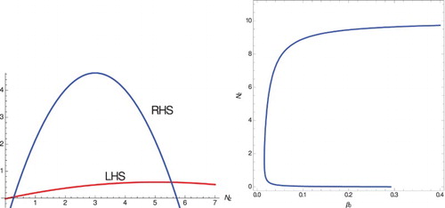
Figure 3. Two intersections of the LHS and RHS of Equation (11(11) $\begin{array}{rl}& \frac{r_1}{({\alpha }_{21}{)}^2{K}_1}\left[K_2\left(1-\frac{m_2}{r_2}\right)-N_2\right]\left[{\alpha }_{21}{K}_1\left(1-\frac{m_1}{r_1}\right)-K_2\left(1-\frac{m_2}{r_2}\right)+(1-{\alpha }_{12}{\alpha }_{21})N_2\right]\\ & ={\alpha }_0(p{N}_2+D)\left[\frac{1}{{\alpha }_{21}}\left[K_2\left(1-\frac{m_2}{r_2}\right)-N_2\right]-\frac{m_1+{\alpha }_0(p{N}_2+D)}{{\beta }_0(p{N}_2+D)}\right].\end{array}$(11) ). Since these happen for positive values of the RHS, $I^{\ast \ast }>0$ for each. Parameter values $r_1=1$, c=0.015, $\mu =1$, p=1, D=35, $m_1=m_2=0.01$, ${\alpha }_{12}=1.5$, ${\alpha }_{21}=1.5$, $K_1=200$, $b_0=40$, $\eta =0.5$, $r_2=2$, $K_2=140$. The equilibria are $S^{\ast \ast }=33.56201$, $I^{\ast \ast }=4.897679$, $N_2^{\ast \ast }=81.61046$ and $S^{\ast \ast }=33.77425$, $I^{\ast \ast }=42.10605$, $N_2^{\ast \ast }=25.47954$. Simulations suggest that these are both unstable.

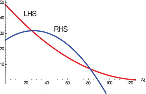
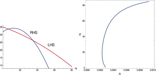
Figure 4. Two intersections of the LHS and RHS of Equation (11(11) $\begin{array}{rl}& \frac{r_1}{({\alpha }_{21}{)}^2{K}_1}\left[K_2\left(1-\frac{m_2}{r_2}\right)-N_2\right]\left[{\alpha }_{21}{K}_1\left(1-\frac{m_1}{r_1}\right)-K_2\left(1-\frac{m_2}{r_2}\right)+(1-{\alpha }_{12}{\alpha }_{21})N_2\right]\\ & ={\alpha }_0(p{N}_2+D)\left[\frac{1}{{\alpha }_{21}}\left[K_2\left(1-\frac{m_2}{r_2}\right)-N_2\right]-\frac{m_1+{\alpha }_0(p{N}_2+D)}{{\beta }_0(p{N}_2+D)}\right].\end{array}$(11) ) (left panel). Since these happen for positive values of the RHS, $I^{\ast \ast }>0$ for each. Parameter values $r_1=0.5$, c=0.01, $\mu =1$, p=1, D=35, $m_1=m_2=0.01$, ${\alpha }_{12}=0.5$, ${\alpha }_{21}=0.8$, $K_1=300$, $b_0=40$, $\eta =0.5$, $r_2=2$, $K_2=100$. The equilibria are $S^{\ast \ast }=50.57192$, $I^{\ast \ast }=30.12703$, $N_2^{\ast \ast }=34.94085$ and $S^{\ast \ast }=50.96722$, $I^{\ast \ast }=65.46346$, $N_2^{\ast \ast }=6.35545$. The two equilibria are obtained through backward bifurcation (right panel). Simulations suggest that the lower one is unstable, while the upper one is locally stable.

3.2. Stability of equilibria of model (5(5) $\begin{array}{rl}{S}^{\prime }& =r_1\left(1-\frac{N_1+{\alpha }_{12}{N}_2}{K_1}\right)N_1-\beta \left(N_2\right)SI-m_{1}S,\\ I^{\prime }& =\beta \left(N_2\right)SI-(m_1+\alpha (N_2\left)\right)I,\\ N_2^{\prime }& =r_2\left(1-\frac{N_2+{\alpha }_{21}{N}_1}{K_2}\right)N_2-m_2{N}_2.\end{array}$(5) )

Model (5(5) $\begin{array}{rl}{S}^{\prime }& =r_1\left(1-\frac{N_1+{\alpha }_{12}{N}_2}{K_1}\right)N_1-\beta \left(N_2\right)SI-m_{1}S,\\ I^{\prime }& =\beta \left(N_2\right)SI-(m_1+\alpha (N_2\left)\right)I,\\ N_2^{\prime }& =r_2\left(1-\frac{N_2+{\alpha }_{21}{N}_1}{K_2}\right)N_2-m_2{N}_2.\end{array}$(5) ) is an ODE model so the local stability of equilibria is determined by examining the eigenvalues of the Jacobian. The following proposition gives the stability of ${\mathcal{E}}_0$ and is not hard to establish.

Proposition 3.5

If ${\mathcal{R}}_1<1$ and ${\mathcal{R}}_2<1,$ then the extinction equilibrium ${\mathcal{E}}_0$ is locally asymptotically stable. If either inequality is reversed, then the extinction equilibrium is unstable.

The stability of ${\mathcal{E}}_1$ is determined by the eigenvalues of the Jacobian evaluated at ${\mathcal{E}}_1$. This Jacobian has the eigenvalues ${\lambda }_1=-\left(r_1/K_1\right){\hat{N}}_1$, ${\lambda }_2=\beta \left(0\right){\hat{N}}_1-(m_1+\alpha (0\left)\right)$ and ${\lambda }_3=r_2(1-{\alpha }_{21}{\hat{N}}_1/K_1)-m_1$. The following proposition gives the stability of ${\mathcal{E}}_1$.

Proposition 3.6

Assume ${\mathcal{R}}_1>1$. Then, equilibrium ${\mathcal{E}}_1$ is locally asymptotically stable if and only if the following two inequalities hold:

1. ${\mathcal{R}}_0<1$,

2. $K_2(1-m_2/r_2)<{\alpha }_{21}{K}_1(1-m_1/r_1)$.

Similarly, we can obtain the stability of equilibrium ${\mathcal{E}}_2$. The Jacobian evaluated at the equilibrium has the eigenvalues ${\lambda }_1=r_1(1-{\alpha }_{12}{\hat{N}}_2/K_1)-m_1$, ${\lambda }_2=-(\mu +\alpha ({\hat{N}}_2\left)\right)$ and ${\lambda }_3=-\left(r_2/K_2\right){\hat{N}}_2$. The following proposition gives the stability of ${\mathcal{E}}_2$.

Proposition 3.7

Assume ${\mathcal{R}}_2>1$. If $K_1\left(1-\frac{m_1}{r_1}\right)<{\alpha }_{12}{K}_2\left(1-\frac{m_2}{r_2}\right),$ then the species 2 equilibrium ${\mathcal{E}}_2$ is locally asymptotically stable. If the above inequality is reversed, then the species 2 equilibrium is unstable.

The stability of ${\mathcal{E}}_{12}$ resembles the stability in the classical Lotka–Volterra model (with an additional condition related to invasion of infected). The following proposition gives the stability of ${\mathcal{E}}_{12}$.

Proposition 3.8

Assume ${\mathcal{E}}_{12}$ exists. Then, ${\mathcal{E}}_{12}$ is locally asymptotically stable if and only if ${\mathcal{R}}_{00}<1$ and $1-{\alpha }_{12}{\alpha }_{21}>0$.

The stability of the species 1 disease equilibrium is given by the following proposition:

Proposition 3.9

Assume ${\mathcal{R}}_1>1$ and ${\mathcal{R}}_0>1$. Then equilibrium ${\mathcal{E}}^{\ast }$ is locally asymptotically stable if and only if ${\hat{\mathcal{R}}}_2<1$.

This result is also not hard to establish. The Jacobian has an eigenvalue ${\lambda }_1=r_2(1-{\alpha }_{21}{N}_1^{\ast }/K_2)-m_2$ which is negative only if ${\hat{\mathcal{R}}}_2<1$. The remaining two eigenvalues are eigenvalues of a 2x2 matrix that has negative trace and positive determinant (see the Proof of Theorem 3.10). Consequently, they have negative real parts. This implies that when species 1 is alone with the pathogen, and the pathogen can persist, then they settle to a stable equilibrium without persistent oscillations.

Next we turn to the stability of the coexistence equilibria. First we show that without the impact of species 2 on the immune system of species 1, the coexistence equilibrium is locally asymptotically stable.

Theorem 3.10

Assume p=0 and the coexistence equilibrium exists. If $1-{\alpha }_{12}{\alpha }_{21}>0,$ then the unique coexistence equilibrium is locally asymptotically stable. If $p=1,$ the coexistence equilibrium can become unstable and oscillations are possible.

Proof.

If p=0 system (5(5) $\begin{array}{rl}{S}^{\prime }& =r_1\left(1-\frac{N_1+{\alpha }_{12}{N}_2}{K_1}\right)N_1-\beta \left(N_2\right)SI-m_{1}S,\\ I^{\prime }& =\beta \left(N_2\right)SI-(m_1+\alpha (N_2\left)\right)I,\\ N_2^{\prime }& =r_2\left(1-\frac{N_2+{\alpha }_{21}{N}_1}{K_2}\right)N_2-m_2{N}_2.\end{array}$(5) ) becomes (14) $\begin{array}{rl}{S}^{\prime }& =r_1\left(1-\frac{N_1+{\alpha }_{12}{N}_2}{K_1}\right)N_1-{\beta }_{0}DSI-m_{1}S,\\ I^{\prime }& ={\beta }_{0}DSI-\left(m_1+{\alpha }_{0}D\right)I,\\ N_2^{\prime }& =r_2\left(1-\frac{N_2+{\alpha }_{21}{N}_1}{K_2}\right)N_2-m_2{N}_2.\end{array}$(14) Computing the Jacobian of the system, we obtain (15) $J=\left(\begin{array}{ccc}-b_{11}& -b_{12}& -\frac{r_1{\alpha }_{12}{N}_1}{K_1}\\ {\beta }_{0}DI& 0& 0\\ -\frac{r_2{\alpha }_{21}{N}_2}{K_2}& -\frac{r_2{\alpha }_{21}{N}_2}{K_2}& -\frac{r_2{N}_2}{K_2}\end{array}\right),$(15) where (16) $\begin{array}{rl}-b_{11}& =r_1\left(1-\frac{S+I+{\alpha }_{12}{N}_2}{K_1}\right)-\frac{r_1(S+I)}{K_1}-{\beta }_{0}DI-m_1\\ & =\frac{1}{S}\left[r_1\left(1-\frac{S+I+{\alpha }_{12}{N}_2}{K_1}\right)(S+I)-{\beta }_{0}DSI-m_{1}S\right.\\ & \left.-\frac{r_1(S+I)}{K_1}-r_1\left(1-\frac{S+I+{\alpha }_{12}{N}_2}{K_1}\right)I\right]\\ & =-\frac{r_1(S+I)}{K_1}-r_1\left(1-\frac{S+I+{\alpha }_{12}{N}_2}{K_1}\right)\frac{I}{S},\\ -b_{12}& =-\frac{r_1(S+I)}{K_1}-\left[r_1\left(1-\frac{S+I+{\alpha }_{12}{N}_2}{K_1}\right)-m_1\right]\frac{S}{I}.\end{array}$(16) Thus, $b_{11}>0$ and $b_{12}>0$. The two are positive since from the equilibrium equation for $N_1$ we have: $\left[r_1\left(1-\frac{S+I+{\alpha }_{12}{N}_2}{K_1}\right)-m_1\right]N_1={\alpha }_{0}DI>0.$ The characteristic equation is given by (17) $\begin{array}{rl}|\lambda I-J|& =\lambda (\lambda +b_{11})\left(\lambda +\frac{r_2{N}_2}{K_2}\right)-\beta I\frac{r_1{\alpha }_{12}{N}_1}{K_1}\frac{r_2{\alpha }_{21}{N}_2}{K_2}+b_{12}\beta I\left(\lambda +\frac{r_2{N}_2}{K_2}\right)\\ & -\frac{r_1{\alpha }_{12}{N}_1}{K_1}\frac{r_2{\alpha }_{21}{N}_2}{K_2}\lambda \\ & ={\lambda }^3+a_2{\lambda }^2+a_1\lambda +a_0,\end{array}$(17) where (18) $\begin{array}{rl}{a}_2& =b_{11}+\frac{r_2{N}_2}{K_2}>0,\\ a_1& =b_{11}\frac{r_2{N}_2}{K_2}-\frac{r_1{\alpha }_{12}{N}_1}{K_1}\frac{r_2{\alpha }_{21}{N}_2}{K_2}+b_{12}\beta I,\\ a_0& =b_{12}\beta I\frac{r_2{N}_2}{K_2}-\beta I\frac{r_1{\alpha }_{12}{N}_1}{K_1}\frac{r_2{\alpha }_{21}{N}_2}{K_2}.\end{array}$(18) Clearly $a_2>0$ and if $1-{\alpha }_{12}{\alpha }_{21}>0$, then $a_1>0$ (since $b_{11}>r_1{N}_1/K_1$). To see that $a_0>0$, we observe (19) $\begin{array}{rl}{a}_0& =\beta I\frac{r_2{N}_2}{K_2}\left(b_{12}-\frac{r_1{\alpha }_{12}{\alpha }_{21}{N}_1}{K_1}\right)\end{array}$(19) (20) $\begin{array}{rl}& =\beta I\frac{r_2{N}_2}{K_2}\left(\frac{r_1{N}_1(1-{\alpha }_{12}{\alpha }_{21})}{K_1}+\left[r_1\left(1-\frac{N_1+{\alpha }_{12}{N}_2}{K_1}\right)-m_1\right]\frac{S}{I}\right)>0.\end{array}$(20) Finally, we check the stability condition $a_2{a}_1-a_0>0$ (21) $\begin{array}{rl}{a}_2{a}_1-a_0& =\left(b_{11}+\frac{r_2{N}_2}{K_2}\right)\left(b_{11}\frac{r_2{N}_2}{K_2}-\frac{r_1{\alpha }_{12}{N}_1}{K_1}\frac{r_2{\alpha }_{21}{N}_2}{K_2}+b_{12}{\beta }_{0}DI\right)\\ & -{\beta }_{0}DI\frac{r_2{N}_2}{K_2}\left(b_{12}-\frac{r_1{\alpha }_{12}{\alpha }_{21}{N}_1}{K_1}\right)\\ & =b_{11}\left(b_{11}\frac{r_2{N}_2}{K_2}-\frac{r_1{\alpha }_{12}{N}_1}{K_1}\frac{r_2{\alpha }_{21}{N}_2}{K_2}+b_{12}{\beta }_{0}DI\right)\\ & +\frac{r_2{N}_2}{K_2}\left(b_{11}\frac{r_2{N}_2}{K_2}-\frac{r_1{\alpha }_{12}{N}_1}{K_1}\frac{r_2{\alpha }_{21}{N}_2}{K_2}+b_{12}{\beta }_{0}DI\right)\\ & -{\beta }_{0}DI\frac{r_2{N}_2}{K_2}{b}_{12}+{\beta }_{0}DI\frac{r_2{N}_2}{K_2}\frac{r_1{\alpha }_{12}{\alpha }_{21}{N}_1}{K_1}\\ & =b_{11}\frac{r_2{N}_2}{K_2}\left(b_{11}-\frac{r_1{\alpha }_{12}{\alpha }_{21}{N}_1}{K_1}\right)\\ & +b_{11}{b}_{12}{\beta }_{0}DI+{\left(\frac{r_2{N}_2}{K_2}\right)}^2\left(b_{11}-\frac{r_1{\alpha }_{12}{\alpha }_{21}{N}_1}{K_1}\right)\\ & +{\beta }_{0}DI\frac{r_2{N}_2}{K_2}\frac{r_1{\alpha }_{12}{\alpha }_{21}{N}_1}{K_1}>0.\end{array}$(21) Since $b_{11}-\frac{r_1{\alpha }_{12}{\alpha }_{21}{N}_1}{K_1}=\frac{r_1{N}_1(1-{\alpha }_{12}{\alpha }_{21})}{K_1}+r_1\left(1-\frac{N_1+{\alpha }_{12}{N}_2}{K_2}\right)\frac{S}{I}>0$ must be positive at equilibrium if $1-{\alpha }_{12}{\alpha }_{21}>0$, because this makes the first term of the last expression positive, while the second term is positive at equilibrium (this follows from the equilibrium equations). Using this condition in Equation (21(21) $\begin{array}{rl}{a}_2{a}_1-a_0& =\left(b_{11}+\frac{r_2{N}_2}{K_2}\right)\left(b_{11}\frac{r_2{N}_2}{K_2}-\frac{r_1{\alpha }_{12}{N}_1}{K_1}\frac{r_2{\alpha }_{21}{N}_2}{K_2}+b_{12}{\beta }_{0}DI\right)\\ & -{\beta }_{0}DI\frac{r_2{N}_2}{K_2}\left(b_{12}-\frac{r_1{\alpha }_{12}{\alpha }_{21}{N}_1}{K_1}\right)\\ & =b_{11}\left(b_{11}\frac{r_2{N}_2}{K_2}-\frac{r_1{\alpha }_{12}{N}_1}{K_1}\frac{r_2{\alpha }_{21}{N}_2}{K_2}+b_{12}{\beta }_{0}DI\right)\\ & +\frac{r_2{N}_2}{K_2}\left(b_{11}\frac{r_2{N}_2}{K_2}-\frac{r_1{\alpha }_{12}{N}_1}{K_1}\frac{r_2{\alpha }_{21}{N}_2}{K_2}+b_{12}{\beta }_{0}DI\right)\\ & -{\beta }_{0}DI\frac{r_2{N}_2}{K_2}{b}_{12}+{\beta }_{0}DI\frac{r_2{N}_2}{K_2}\frac{r_1{\alpha }_{12}{\alpha }_{21}{N}_1}{K_1}\\ & =b_{11}\frac{r_2{N}_2}{K_2}\left(b_{11}-\frac{r_1{\alpha }_{12}{\alpha }_{21}{N}_1}{K_1}\right)\\ & +b_{11}{b}_{12}{\beta }_{0}DI+{\left(\frac{r_2{N}_2}{K_2}\right)}^2\left(b_{11}-\frac{r_1{\alpha }_{12}{\alpha }_{21}{N}_1}{K_1}\right)\\ & +{\beta }_{0}DI\frac{r_2{N}_2}{K_2}\frac{r_1{\alpha }_{12}{\alpha }_{21}{N}_1}{K_1}>0.\end{array}$(21) ) proves that $a_2{a}_1-a_0>0$, which completes the proof in the case p=0.

For $p\ne 0$, we illustrate a case giving oscillations in Figure 5. Although this figure was initiated far from the equilibrium, the same final state is reached starting very close to the equilibrium, and it can be shown that the Jacobian (with p=1) has eigenvalues with positive real parts, so the equilibrium is locally unstable. For these parameters, in the absence of the disease, species 1 out-competes and eliminates species 2, but the presence of the disease in species 1 reduces $N_1$ to a level at which species 2 can invade. So, Figure 5 shows periods of very low I during which S increases and $N_2$ decreases due to the superior competitive ability of species 1. However, eventually S gets high enough to cause a disease outbreak, which leads to a decrease in $N_1$ to a level that allows $N_2$ to increase again. As $N_2$ increases, so does the parasite load in infected hosts, increasing the infection rate and infected death rate, decreasing S and ultimately I, which reaches a very low level again, and the cycle repeats. The effect of species 2 on species 1's immunity causes positive feedback when $N_2$ is increasing, because this increase accelerates the decline in $N_1$ due to infection (without this effect, S, I and $N_2$ reach a stable equilibrium)

Figure 5. Oscillations in system (5(5) $\begin{array}{rl}{S}^{\prime }& =r_1\left(1-\frac{N_1+{\alpha }_{12}{N}_2}{K_1}\right)N_1-\beta \left(N_2\right)SI-m_{1}S,\\ I^{\prime }& =\beta \left(N_2\right)SI-(m_1+\alpha (N_2\left)\right)I,\\ N_2^{\prime }& =r_2\left(1-\frac{N_2+{\alpha }_{21}{N}_1}{K_2}\right)N_2-m_2{N}_2.\end{array}$(5) ). Parameter values are: $r_1=0.01$, c=0.02, $\mu =0.2$, p=1, D=10, $m_1=0.001$, $m_2=0.3$, ${\alpha }_{12}=0.9$, ${\alpha }_{21}=0.9$, $K_1=100$, $b_0=30$, $\eta =0.5$, $r_2=0.4$, $K_2=180$, which makes $a_2{a}_1-a_0$ equal to $-3.5\ast {10}^{-6}$. $S\left(t\right)$ is in blue, $I\left(t\right)$ is in red and $N_2\left(t\right)$ is in dashed black.

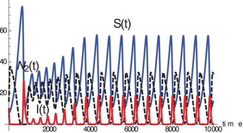
Figure 5 assumed that β and α were linear functions of $V^{\ast }$. If instead they were both assumed to be saturating functions of $V^{\ast }$, then the oscillations in Figure 5 tend to be reduced as the amount of saturation increases. This is not surprising, since if values of $V^{\ast }$ are such that both β and α are completely saturated, then β and α are constant and the system reduces to that of (5(5) $\begin{array}{rl}{S}^{\prime }& =r_1\left(1-\frac{N_1+{\alpha }_{12}{N}_2}{K_1}\right)N_1-\beta \left(N_2\right)SI-m_{1}S,\\ I^{\prime }& =\beta \left(N_2\right)SI-(m_1+\alpha (N_2\left)\right)I,\\ N_2^{\prime }& =r_2\left(1-\frac{N_2+{\alpha }_{21}{N}_1}{K_2}\right)N_2-m_2{N}_2.\end{array}$(5) ) with $p=0$, which does not oscillate. We performed simulations with the parameters of Figure 5 but with saturating functions for $\beta \left(V^{\ast }\right)$ and $\alpha \left(V^{\ast }\right)$ (each of the linear functions above was divided by $1+u{V}^{\ast }$). Oscillations were still present with modest amounts of saturation (up to u=4, at which saturation reduced the values of β and α to about half their linear values). If only α saturated, then very little saturation (u=1) stabilized the dynamics, while if only β saturated, the system still oscillated at u=8 (but saturation in this case also decreased $N_2^{\ast }$ and therefore $V^{\ast }$). Saturation with differing strengths (stronger for β) could give oscillations with greater amounts of saturation (e.g. u=8 for α and u=16 for β) than equal saturation or saturation of only one function. Likewise, the backward bifurcation of Figure 2 occurred up to moderate amounts of saturation (about u=0.003 with equal saturation, which reduced each function to 30% of its linear value at the positive stable equilibrium), but was not present for greater degrees of equal saturation. In this case, with saturation of only one function, backward bifurcation persisted for much greater saturation of α (higher than u=0.05, which reduced α to less than 5% of its linear value at the positive stable equilibrium) than of β (only up to about u=0.001). In this case, saturation of α allowed bifurcation for higher saturation of β, but not the reverse.

A summary of equilibria and their stability for system (5(5) $\begin{array}{rl}{S}^{\prime }& =r_1\left(1-\frac{N_1+{\alpha }_{12}{N}_2}{K_1}\right)N_1-\beta \left(N_2\right)SI-m_{1}S,\\ I^{\prime }& =\beta \left(N_2\right)SI-(m_1+\alpha (N_2\left)\right)I,\\ N_2^{\prime }& =r_2\left(1-\frac{N_2+{\alpha }_{21}{N}_1}{K_2}\right)N_2-m_2{N}_2.\end{array}$(5) ) is given in Table 4.

Table 4. Summary of equilibria and their stabilities for system (5(5) $\begin{array}{rl}{S}^{\prime }& =r_1\left(1-\frac{N_1+{\alpha }_{12}{N}_2}{K_1}\right)N_1-\beta \left(N_2\right)SI-m_{1}S,\\ I^{\prime }& =\beta \left(N_2\right)SI-(m_1+\alpha (N_2\left)\right)I,\\ N_2^{\prime }& =r_2\left(1-\frac{N_2+{\alpha }_{21}{N}_1}{K_2}\right)N_2-m_2{N}_2.\end{array}$(5) ).

Eq.	Exists if	Stable if	Unstable if
${\mathcal{E}}_0$	always	${\mathcal{R}}_1<1$ and ${\mathcal{R}}_2<1$	${\mathcal{R}}_1>1$ or ${\mathcal{R}}_2>1$
${\mathcal{E}}_{10}$	${\mathcal{R}}_1>1$	${\mathcal{R}}_0<1$ and	${\mathcal{R}}_0>1$ or
		${\displaystyle K_2\left(1-\frac{m_2}{r_2}\right)<{\alpha }_{21}{K}_1\left(1-\frac{m_1}{r_1}\right)}$	${\displaystyle K_2\left(1-\frac{m_2}{r_2}\right)>{\alpha }_{21}{K}_1\left(1-\frac{m_1}{r_1}\right)}$
${\mathcal{E}}_2$	${\mathcal{R}}_2>1$	$K_1\left(1-{\displaystyle \frac{m_1}{r_1}}\right)<{\alpha }_{12}{K}_2\left(1-{\displaystyle \frac{m_2}{r_2}}\right)$	$K_1\left(1-{\displaystyle \frac{m_1}{r_1}}\right)>{\alpha }_{12}{K}_2\left(1-{\displaystyle \frac{m_2}{r_2}}\right)$
${\mathcal{E}}_{12}$	$\left\{\begin{array}{l}{K}_1\left(1-{\displaystyle \frac{m_1}{r_1}}\right)>{\alpha }_{12}{K}_2\left(1-{\displaystyle \frac{m_2}{r_2}}\right)\\ K_2\left(1-{\displaystyle \frac{m_2}{r_2}}\right)>{\alpha }_{21}{K}_1\left(1-{\displaystyle \frac{m_1}{r_1}}\right)\end{array}\right.$	${\mathcal{R}}_{00}<1$	${\mathcal{R}}_{00}>1$
${\mathcal{E}}_{12}$	$\left\{\begin{array}{l}{K}_1\left(1-{\displaystyle \frac{m_1}{r_1}}\right)<{\alpha }_{12}{K}_2\left(1-{\displaystyle \frac{m_2}{r_2}}\right)\\ K_2\left(1-{\displaystyle \frac{m_2}{r_2}}\right)<{\alpha }_{21}{K}_1\left(1-{\displaystyle \frac{m_1}{r_1}}\right)\end{array}\right.$	–	always
${\mathcal{E}}^{\ast }$	${\mathcal{R}}_1>1$ and ${\mathcal{R}}_0>1$	${\hat{\mathcal{R}}}_2<1$	${\hat{\mathcal{R}}}_2>1$
${\mathcal{E}}^{\ast \ast }$	${\mathcal{R}}_i>1$, ${\hat{\mathcal{R}}}_2>1$ or ${\mathcal{R}}_{00}>1$	$\alpha \left(\tau \right)=0$ or p=0,
		and ${\alpha }_{12}{\alpha }_{21}<1$

4. Equilibria of the full model

In this section, we investigate the equilibria of the more complex model (1(1) $\begin{array}{rl}{V}_t(\tau ,t)+V_{\tau }(\tau ,t)& =r_{v}V(\tau ,t)(1-qV(\tau ,t\left)\right)-aV(\tau ,t)z(\tau ,t),\\ z_t(\tau ,t)+z_{\tau }(\tau ,t)& =\frac{b_{0}V(\tau ,t)z(\tau ,t)}{\left(p{N}_2\right(t)+D)(1+b_{2}V)}-\mu z(\tau ,t).\end{array}$(1) )–(4(4) $\begin{array}{rl}{S}^{\prime }& =r_1\left(1-\frac{N_1+{\alpha }_{12}{N}_2}{K_1}\right)N_1-S\left(t\right){\int }_0^{\mathrm{\infty }}\beta \left(\tau \right)i(\tau ,t)\mathrm{d}\tau -m_{1}S\left(t\right),\\ i_{\tau }(\tau ,t)+i_t(\tau ,t)& =-(m_1+\alpha (\tau )+\gamma (\tau \left)\right)i(\tau ,t),\\ i(0,t)& =S\left(t\right){\int }_0^{\mathrm{\infty }}\beta \left(\tau \right)i(\tau ,t)\mathrm{d}\tau ,\\ R^{\prime }& ={\int }_0^{\mathrm{\infty }}\gamma \left(\tau \right)i(\tau ,t)\mathrm{d}\tau -m_{1}R,\\ N_2^{\prime }\left(t\right)& =r_2\left(1-\frac{N_2+{\alpha }_{21}{N}_1}{K_2}\right)N_2-m_2{N}_2.\end{array}$(4) ). Equilibria are time-independent solutions. They solve the system: (22) $\begin{array}{rl}{V}_{\tau }\left(\tau \right)& =r_{v}V\left(\tau \right)(1-qV(\tau \left)\right)-aV\left(\tau \right)z\left(\tau \right),\\ z_{\tau }\left(\tau \right)& =\frac{b_{0}V\left(\tau \right)z\left(\tau \right)}{(p{N}_2+D)(1+b_{2}V)}-\mu z\left(\tau \right),\\ V\left(0\right)& =V_0,\\ z\left(0\right)& =z_0,\\ 0& =r_1\left(1-\frac{N_1+{\alpha }_{12}{N}_2}{K_1}\right)N_1-S{\int }_0^{\mathrm{\infty }}\beta \left(\tau \right)i\left(\tau \right)\mathrm{d}\tau -m_{1}S,\\ i_{\tau }\left(\tau \right)& =-(m_1+\alpha (\tau )+\gamma (\tau \left)\right)i\left(\tau \right),\\ i\left(0\right)& =S{\int }_0^{\mathrm{\infty }}\beta \left(\tau \right)i\left(\tau \right)\mathrm{d}\tau ,\\ 0& ={\int }_0^{\mathrm{\infty }}\gamma \left(\tau \right)i\left(\tau \right)\mathrm{d}\tau -m_{1}R,\\ 0& =r_2\left(1-\frac{N_2+{\alpha }_{21}{N}_1}{K_2}\right)N_2-m_2{N}_2.\end{array}$(22)

Note that this is the between-host equilibrium (in contrast to the within-host equilibrium of the previous section). At this equilibrium, the values of $N_2$, S, R and number of infected hosts are assumed constant (independent of t). However, susceptible hosts are constantly becoming infected (balanced by death and recovery of infected hosts), and the values of V and z within infected hosts are given by Equation (1(1) $\begin{array}{rl}{V}_t(\tau ,t)+V_{\tau }(\tau ,t)& =r_{v}V(\tau ,t)(1-qV(\tau ,t\left)\right)-aV(\tau ,t)z(\tau ,t),\\ z_t(\tau ,t)+z_{\tau }(\tau ,t)& =\frac{b_{0}V(\tau ,t)z(\tau ,t)}{\left(p{N}_2\right(t)+D)(1+b_{2}V)}-\mu z(\tau ,t).\end{array}$(1) ) assuming $N_2$ fixed at its equilibrium. This gives the first two equations, which are now ODEs in terms of time-since-infection τ.

In system above, we assume $V_0>0$ and $z_0>0$. This assumption is equivalent to the assumption that the within-host equations describe the dynamics, given an infection. Thus, the equilibrial values of V and z are positive, independently whether there are infected individuals in the population. In reality, $V_0$ is undefined if I=0 and $V_0>0$ if I>0 but to simplify matters we will always assume that $V_0>0$.

System (22(22) $\begin{array}{rl}{V}_{\tau }\left(\tau \right)& =r_{v}V\left(\tau \right)(1-qV(\tau \left)\right)-aV\left(\tau \right)z\left(\tau \right),\\ z_{\tau }\left(\tau \right)& =\frac{b_{0}V\left(\tau \right)z\left(\tau \right)}{(p{N}_2+D)(1+b_{2}V)}-\mu z\left(\tau \right),\\ V\left(0\right)& =V_0,\\ z\left(0\right)& =z_0,\\ 0& =r_1\left(1-\frac{N_1+{\alpha }_{12}{N}_2}{K_1}\right)N_1-S{\int }_0^{\mathrm{\infty }}\beta \left(\tau \right)i\left(\tau \right)\mathrm{d}\tau -m_{1}S,\\ i_{\tau }\left(\tau \right)& =-(m_1+\alpha (\tau )+\gamma (\tau \left)\right)i\left(\tau \right),\\ i\left(0\right)& =S{\int }_0^{\mathrm{\infty }}\beta \left(\tau \right)i\left(\tau \right)\mathrm{d}\tau ,\\ 0& ={\int }_0^{\mathrm{\infty }}\gamma \left(\tau \right)i\left(\tau \right)\mathrm{d}\tau -m_{1}R,\\ 0& =r_2\left(1-\frac{N_2+{\alpha }_{21}{N}_1}{K_2}\right)N_2-m_2{N}_2.\end{array}$(22) ) has the extinction equilibrium ${\mathcal{E}}_0=\left(V\right(\tau ),z(\tau ),0,0,0,0)$ where $V\left(\tau \right),z\left(\tau \right)$ are the solutions of the within-host equations with $N_2=0$. This equilibrium always exists. (Since there are no hosts in this case, V and z are irrelevant, but they can still be defined since they describe the within-host dynamics if there were an infected host.)

Next, we have the species 1-free equilibrium ${\mathcal{E}}_2=\left(\hat{V}\right(\tau ),\hat{z}(\tau ),0,0,0,{\hat{N}}_2)$ where $\hat{V}\left(\tau \right),\hat{z}\left(\tau \right)$ are the solutions of the within-host equations computed with $N_2={\hat{N}}_2$ and ${\hat{N}}_2=K_2(1-m_2/r_2)$, which exists only if $r_2>m_2$. Symmetrically, system (22(22) $\begin{array}{rl}{V}_{\tau }\left(\tau \right)& =r_{v}V\left(\tau \right)(1-qV(\tau \left)\right)-aV\left(\tau \right)z\left(\tau \right),\\ z_{\tau }\left(\tau \right)& =\frac{b_{0}V\left(\tau \right)z\left(\tau \right)}{(p{N}_2+D)(1+b_{2}V)}-\mu z\left(\tau \right),\\ V\left(0\right)& =V_0,\\ z\left(0\right)& =z_0,\\ 0& =r_1\left(1-\frac{N_1+{\alpha }_{12}{N}_2}{K_1}\right)N_1-S{\int }_0^{\mathrm{\infty }}\beta \left(\tau \right)i\left(\tau \right)\mathrm{d}\tau -m_{1}S,\\ i_{\tau }\left(\tau \right)& =-(m_1+\alpha (\tau )+\gamma (\tau \left)\right)i\left(\tau \right),\\ i\left(0\right)& =S{\int }_0^{\mathrm{\infty }}\beta \left(\tau \right)i\left(\tau \right)\mathrm{d}\tau ,\\ 0& ={\int }_0^{\mathrm{\infty }}\gamma \left(\tau \right)i\left(\tau \right)\mathrm{d}\tau -m_{1}R,\\ 0& =r_2\left(1-\frac{N_2+{\alpha }_{21}{N}_1}{K_2}\right)N_2-m_2{N}_2.\end{array}$(22) ) has a no-disease, no-species-2 equilibrium ${\mathcal{E}}_1=\left(V\right(\tau ),z(\tau ),{\hat{N}}_1,0,0,0)$ where ${\hat{N}}_1=K_1(1-m_1/r_1)$. This equilibrium exists only if $r_1>m_1$.

Proposition 4.1

Equilibrium ${\mathcal{E}}_1$ exists iff ${\mathcal{R}}_1>1$. Equilibrium ${\mathcal{E}}_2$ exists if and only if ${\mathcal{R}}_2>1$.

Assume ${\mathcal{R}}_1>1$ and ${\mathcal{R}}_2>1$. Then the system has another disease-free equilibrium: the no-disease coexistence equilibrium ${\mathcal{E}}_{12}=\left(\overline{V}\right(\tau ),\overline{z}(\tau ),{\overline{N}}_1,0,0,{\overline{N}}_2)$, where $\overline{V}\left(\tau \right),\overline{z}\left(\tau \right)$ are solutions of the within-host equations with $N_2={\overline{N}}_2$ and ${\overline{N}}_1$ and ${\overline{N}}_2$ are defined in Equation (6(6) $\begin{array}{rl}{\overline{N}}_1& =\frac{K_1\left(1-{\displaystyle \frac{m_1}{r_1}}\right)-{\alpha }_{12}{K}_2\left(1-{\displaystyle \frac{m_2}{r_2}}\right)}{1-{\alpha }_{12}{\alpha }_{21}},\\ {\overline{N}}_2& =\frac{K_2\left(1-{\displaystyle \frac{m_2}{r_2}}\right)-{\alpha }_{21}{K}_1\left(1-{\displaystyle \frac{m_1}{r_1}}\right)}{1-{\alpha }_{12}{\alpha }_{21}}.\end{array}$(6) ). Equilibrium ${\mathcal{E}}_{12}$ exists under the conditions specified in Proposition 3.2.

Now, we turn to the existence of the endemic equilibria (those including the disease). First, we consider the endemic equilibrium without species 2 ${\mathcal{E}}^{\ast }=\left(V^{\ast }\right(\tau ),z^{\ast }(\tau ),S^{\ast },i^{\ast }(\tau ),R^{\ast },0)$, where $V^{\ast }\left(\tau \right)$ and $z^{\ast }\left(\tau \right)$ are the solutions of the first two differential equations in Equation (22(22) $\begin{array}{rl}{V}_{\tau }\left(\tau \right)& =r_{v}V\left(\tau \right)(1-qV(\tau \left)\right)-aV\left(\tau \right)z\left(\tau \right),\\ z_{\tau }\left(\tau \right)& =\frac{b_{0}V\left(\tau \right)z\left(\tau \right)}{(p{N}_2+D)(1+b_{2}V)}-\mu z\left(\tau \right),\\ V\left(0\right)& =V_0,\\ z\left(0\right)& =z_0,\\ 0& =r_1\left(1-\frac{N_1+{\alpha }_{12}{N}_2}{K_1}\right)N_1-S{\int }_0^{\mathrm{\infty }}\beta \left(\tau \right)i\left(\tau \right)\mathrm{d}\tau -m_{1}S,\\ i_{\tau }\left(\tau \right)& =-(m_1+\alpha (\tau )+\gamma (\tau \left)\right)i\left(\tau \right),\\ i\left(0\right)& =S{\int }_0^{\mathrm{\infty }}\beta \left(\tau \right)i\left(\tau \right)\mathrm{d}\tau ,\\ 0& ={\int }_0^{\mathrm{\infty }}\gamma \left(\tau \right)i\left(\tau \right)\mathrm{d}\tau -m_{1}R,\\ 0& =r_2\left(1-\frac{N_2+{\alpha }_{21}{N}_1}{K_2}\right)N_2-m_2{N}_2.\end{array}$(22) ) for $N_2=0$ [other quantities in this section with an asterisk are evaluated at $N_2=0$, $V=V^{\ast }\left(\tau \right)$ and $z=z^{\ast }\left(\tau \right)$]. We define the probability of remaining in the infected class τ units after infection as (23) ${\pi }^{\ast }\left(\tau \right)={\mathrm{e}}^{-{\int }_0^{\tau }(m_1+{\alpha }^{\ast }(\eta )+{\gamma }^{\ast }(\eta \left)\right)\mathrm{d}\eta }.$(23) The solution of the third differential equation in system (22(22) $\begin{array}{rl}{V}_{\tau }\left(\tau \right)& =r_{v}V\left(\tau \right)(1-qV(\tau \left)\right)-aV\left(\tau \right)z\left(\tau \right),\\ z_{\tau }\left(\tau \right)& =\frac{b_{0}V\left(\tau \right)z\left(\tau \right)}{(p{N}_2+D)(1+b_{2}V)}-\mu z\left(\tau \right),\\ V\left(0\right)& =V_0,\\ z\left(0\right)& =z_0,\\ 0& =r_1\left(1-\frac{N_1+{\alpha }_{12}{N}_2}{K_1}\right)N_1-S{\int }_0^{\mathrm{\infty }}\beta \left(\tau \right)i\left(\tau \right)\mathrm{d}\tau -m_{1}S,\\ i_{\tau }\left(\tau \right)& =-(m_1+\alpha (\tau )+\gamma (\tau \left)\right)i\left(\tau \right),\\ i\left(0\right)& =S{\int }_0^{\mathrm{\infty }}\beta \left(\tau \right)i\left(\tau \right)\mathrm{d}\tau ,\\ 0& ={\int }_0^{\mathrm{\infty }}\gamma \left(\tau \right)i\left(\tau \right)\mathrm{d}\tau -m_{1}R,\\ 0& =r_2\left(1-\frac{N_2+{\alpha }_{21}{N}_1}{K_2}\right)N_2-m_2{N}_2.\end{array}$(22) ) is given by: $i^{\ast }\left(\tau \right)=i^{\ast }\left(0\right){\pi }^{\ast }\left(\tau \right)$. Substituting this form in the equation for $i\left(0\right)$, we obtain $S^{\ast }$. From the equation for the recovered individuals, we have (24) $S^{\ast }=\frac{1}{{\int }_0^{\mathrm{\infty }}{\beta }^{\ast }\left(\tau \right){\pi }^{\ast }\left(\tau \right)\mathrm{d}\tau }{R}^{\ast }=\frac{i^{\ast }\left(0\right){\int }_0^{\mathrm{\infty }}{\gamma }^{\ast }\left(\tau \right){\pi }^{\ast }\left(\tau \right)\mathrm{d}\tau }{m_1}.$(24) Denote by ${\mathrm{\Pi }}^{\ast }={\int }_0^{\mathrm{\infty }}{\pi }^{\ast }\left(\tau \right)\mathrm{d}\tau {\mathrm{\Gamma }}^{\ast }=\frac{1}{m_1}{\int }_0^{\mathrm{\infty }}{\gamma }^{\ast }\left(\tau \right){\pi }^{\ast }\left(\tau \right)\mathrm{d}\tau .$ Expressing $i^{\ast }\left(0\right)$ from the equation for the total population size of species 1 $N_1^{\ast }=S^{\ast }+{\int }_0^{\mathrm{\infty }}{i}^{\ast }\left(\tau \right)d\tau +R^{\ast }$, we have (25) $i^{\ast }\left(0\right)=\frac{N_1^{\ast }-S^{\ast }}{{\mathrm{\Pi }}^{\ast }+{\mathrm{\Gamma }}^{\ast }}.$(25) Substituting $i^{\ast }\left(0\right)$ into the fifth equation of system (22(22) $\begin{array}{rl}{V}_{\tau }\left(\tau \right)& =r_{v}V\left(\tau \right)(1-qV(\tau \left)\right)-aV\left(\tau \right)z\left(\tau \right),\\ z_{\tau }\left(\tau \right)& =\frac{b_{0}V\left(\tau \right)z\left(\tau \right)}{(p{N}_2+D)(1+b_{2}V)}-\mu z\left(\tau \right),\\ V\left(0\right)& =V_0,\\ z\left(0\right)& =z_0,\\ 0& =r_1\left(1-\frac{N_1+{\alpha }_{12}{N}_2}{K_1}\right)N_1-S{\int }_0^{\mathrm{\infty }}\beta \left(\tau \right)i\left(\tau \right)\mathrm{d}\tau -m_{1}S,\\ i_{\tau }\left(\tau \right)& =-(m_1+\alpha (\tau )+\gamma (\tau \left)\right)i\left(\tau \right),\\ i\left(0\right)& =S{\int }_0^{\mathrm{\infty }}\beta \left(\tau \right)i\left(\tau \right)\mathrm{d}\tau ,\\ 0& ={\int }_0^{\mathrm{\infty }}\gamma \left(\tau \right)i\left(\tau \right)\mathrm{d}\tau -m_{1}R,\\ 0& =r_2\left(1-\frac{N_2+{\alpha }_{21}{N}_1}{K_2}\right)N_2-m_2{N}_2.\end{array}$(22) ), we obtain the following equation for $N_1^{\ast }$: (26) $r_1\left(1-\frac{N_1^{\ast }}{K_1}\right)N_1^{\ast }=\frac{N_1^{\ast }-S^{\ast }}{{\mathrm{\Pi }}^{\ast }+{\mathrm{\Gamma }}^{\ast }}+m_1{S}^{\ast }.$(26) We define the reproduction number, under the assumption that ${\mathcal{R}}_1>1$, as follows: ${\mathcal{R}}_0=K_1\left(1-\frac{m_1}{r_1}\right){\int }_0^{\mathrm{\infty }}{\beta }^{\ast }\left(\tau \right){\pi }^{\ast }\left(\tau \right)\mathrm{d}\tau .$

Proposition 4.2

Assume ${\mathcal{R}}_1>1$. Equation (26(26) $r_1\left(1-\frac{N_1^{\ast }}{K_1}\right)N_1^{\ast }=\frac{N_1^{\ast }-S^{\ast }}{{\mathrm{\Pi }}^{\ast }+{\mathrm{\Gamma }}^{\ast }}+m_1{S}^{\ast }.$(26) ) has a unique solution $N_1^{\ast }>S^{\ast }$ if and only if ${\mathcal{R}}_0>1$.

Proof.

Rewriting Equation (26(26) $r_1\left(1-\frac{N_1^{\ast }}{K_1}\right)N_1^{\ast }=\frac{N_1^{\ast }-S^{\ast }}{{\mathrm{\Pi }}^{\ast }+{\mathrm{\Gamma }}^{\ast }}+m_1{S}^{\ast }.$(26) ) as a quadratic equation, we have $\frac{r_1}{K_1}{N}_1^{\ast }{}^2+\left(\frac{1}{{\mathrm{\Pi }}^{\ast }+{\mathrm{\Gamma }}^{\ast }}-r_1\right)N_1^{\ast }+\left(m_1-\frac{1}{{\mathrm{\Pi }}^{\ast }+{\mathrm{\Gamma }}^{\ast }}\right)S^{\ast }=0.$ Direct integration implies that $m_1({\mathrm{\Pi }}^{\ast }+{\mathrm{\Gamma }}^{\ast })<1.$

Hence, the constant term in the above quadratic equation is negative. Therefore, the quadratic equation for $N_1^{\ast }$ has exactly one positive root. Denote by $p_1\left(N_1^{\ast }\right)$ the left-hand side in Equation (26(26) $r_1\left(1-\frac{N_1^{\ast }}{K_1}\right)N_1^{\ast }=\frac{N_1^{\ast }-S^{\ast }}{{\mathrm{\Pi }}^{\ast }+{\mathrm{\Gamma }}^{\ast }}+m_1{S}^{\ast }.$(26) ) and by $p_2\left(N_1^{\ast }\right)$ the right-hand side. Assume first that ${\mathcal{R}}_0>1$. Then $S^{\ast }<K_1(1-m_1/r_1)<K_1$. Hence, $p_1\left(S^{\ast }\right)>p_2\left(S^{\ast }\right)$ and $p_1\left(K_1\right)<p_2\left(K_1\right)$. Thus, Equation (26(26) $r_1\left(1-\frac{N_1^{\ast }}{K_1}\right)N_1^{\ast }=\frac{N_1^{\ast }-S^{\ast }}{{\mathrm{\Pi }}^{\ast }+{\mathrm{\Gamma }}^{\ast }}+m_1{S}^{\ast }.$(26) ) has a unique solution in the interval $(S^{\ast },K_1)$. Thus, there exists a unique $N_1^{\ast }>S^{\ast }$. Now, assume ${\mathcal{R}}_0<1$. Then $S^{\ast }>K_1(1-m_1/r_1)$. Hence, $p_1\left(S^{\ast }\right)<p_2\left(S^{\ast }\right)$ and $p_1\left(K_1\right)<p_2\left(K_1\right)$. Thus, Equation (26(26) $r_1\left(1-\frac{N_1^{\ast }}{K_1}\right)N_1^{\ast }=\frac{N_1^{\ast }-S^{\ast }}{{\mathrm{\Pi }}^{\ast }+{\mathrm{\Gamma }}^{\ast }}+m_1{S}^{\ast }.$(26) ) does not have a root in the interval $(S^{\ast },K_1)$. We conclude that there exists a unique $N_1^{\ast }>S^{\ast }$, at which $i^{\ast }>0$.

Finally, we consider the coexistence equilibrium ${\mathcal{E}}^{\ast \ast }=\left(V^{\ast \ast }\right(\tau ),z^{\ast \ast }(\tau ),S^{\ast \ast },i^{\ast \ast }(\tau ),R^{\ast \ast },N_2^{\ast \ast })$, where $V^{\ast \ast }\left(\tau \right)$ and $z^{\ast \ast }\left(\tau \right)$ are the solutions of the first two differential equations in Equation (22(22) $\begin{array}{rl}{V}_{\tau }\left(\tau \right)& =r_{v}V\left(\tau \right)(1-qV(\tau \left)\right)-aV\left(\tau \right)z\left(\tau \right),\\ z_{\tau }\left(\tau \right)& =\frac{b_{0}V\left(\tau \right)z\left(\tau \right)}{(p{N}_2+D)(1+b_{2}V)}-\mu z\left(\tau \right),\\ V\left(0\right)& =V_0,\\ z\left(0\right)& =z_0,\\ 0& =r_1\left(1-\frac{N_1+{\alpha }_{12}{N}_2}{K_1}\right)N_1-S{\int }_0^{\mathrm{\infty }}\beta \left(\tau \right)i\left(\tau \right)\mathrm{d}\tau -m_{1}S,\\ i_{\tau }\left(\tau \right)& =-(m_1+\alpha (\tau )+\gamma (\tau \left)\right)i\left(\tau \right),\\ i\left(0\right)& =S{\int }_0^{\mathrm{\infty }}\beta \left(\tau \right)i\left(\tau \right)\mathrm{d}\tau ,\\ 0& ={\int }_0^{\mathrm{\infty }}\gamma \left(\tau \right)i\left(\tau \right)\mathrm{d}\tau -m_{1}R,\\ 0& =r_2\left(1-\frac{N_2+{\alpha }_{21}{N}_1}{K_2}\right)N_2-m_2{N}_2.\end{array}$(22) ) for $N_2=N_2^{\ast \ast }$ [other quantities in this section with two asterisks are evaluated at $N_2=N_2^{\ast \ast }$, $V=V^{\ast \ast }\left(\tau \right)$ and $z=z^{\ast \ast }\left(\tau \right)$].

We define the reproduction number of the disease, where the disease-free population consists of both competitors (27) ${\mathcal{R}}_{00}={\overline{N}}_1{\int }_0^{\mathrm{\infty }}\overline{\beta }\left(\tau \right)\overline{\pi }\left(\tau \right)\mathrm{d}\tau ,$(27) where $\overline{\beta }\left(\tau \right)=\beta (\tau ,{\overline{N}}_2)$, $\overline{\alpha }\left(\tau \right)=\alpha (\tau ,{\overline{N}}_2)$, $\overline{\gamma }\left(\tau \right)=\gamma (\tau ,{\overline{N}}_2)$. From the last equation in Equation (22(22) $\begin{array}{rl}{V}_{\tau }\left(\tau \right)& =r_{v}V\left(\tau \right)(1-qV(\tau \left)\right)-aV\left(\tau \right)z\left(\tau \right),\\ z_{\tau }\left(\tau \right)& =\frac{b_{0}V\left(\tau \right)z\left(\tau \right)}{(p{N}_2+D)(1+b_{2}V)}-\mu z\left(\tau \right),\\ V\left(0\right)& =V_0,\\ z\left(0\right)& =z_0,\\ 0& =r_1\left(1-\frac{N_1+{\alpha }_{12}{N}_2}{K_1}\right)N_1-S{\int }_0^{\mathrm{\infty }}\beta \left(\tau \right)i\left(\tau \right)\mathrm{d}\tau -m_{1}S,\\ i_{\tau }\left(\tau \right)& =-(m_1+\alpha (\tau )+\gamma (\tau \left)\right)i\left(\tau \right),\\ i\left(0\right)& =S{\int }_0^{\mathrm{\infty }}\beta \left(\tau \right)i\left(\tau \right)\mathrm{d}\tau ,\\ 0& ={\int }_0^{\mathrm{\infty }}\gamma \left(\tau \right)i\left(\tau \right)\mathrm{d}\tau -m_{1}R,\\ 0& =r_2\left(1-\frac{N_2+{\alpha }_{21}{N}_1}{K_2}\right)N_2-m_2{N}_2.\end{array}$(22) ), we express $N_2^{\ast \ast }$ in terms of $N_1^{\ast \ast }$: $N_2^{\ast \ast }=K_2\left(1-\frac{m_2}{r_2}\right)-{\alpha }_{21}{N}_1^{\ast \ast }.$ We have $S^{\ast \ast }=\frac{1}{{\int }_0^{\mathrm{\infty }}\beta \left(\tau \right)\pi \left(\tau \right)\mathrm{d}\tau }{R}^{\ast \ast }=\frac{i^{\ast \ast }\left(0\right){\int }_0^{\mathrm{\infty }}\gamma \left(\tau \right)\pi \left(\tau \right)\mathrm{d}\tau }{m_1}$ and $\pi \left(\tau \right)$, Π, Γ and $i^{\ast \ast }\left(0\right)$ are defined as in the previous section. However, we note that $S^{\ast \ast }\ne S^{\ast }$ as $S^{\ast }$ is computed at $N_2=0$, while $S^{\ast \ast }$ is computed at the yet unknown $N_2^{\ast \ast }$. The same is true for $R^{\ast \ast },\mathrm{\Pi }$, Γ and $i^{\ast \ast }\left(0\right)$. Note also that $\beta \left(\tau \right)=\beta (\tau ,N_2^{\ast \ast })$ and $\gamma \left(\tau \right)=\gamma (\tau ,N_2^{\ast \ast })$. Thus, from the first equation in Equation (22(22) $\begin{array}{rl}{V}_{\tau }\left(\tau \right)& =r_{v}V\left(\tau \right)(1-qV(\tau \left)\right)-aV\left(\tau \right)z\left(\tau \right),\\ z_{\tau }\left(\tau \right)& =\frac{b_{0}V\left(\tau \right)z\left(\tau \right)}{(p{N}_2+D)(1+b_{2}V)}-\mu z\left(\tau \right),\\ V\left(0\right)& =V_0,\\ z\left(0\right)& =z_0,\\ 0& =r_1\left(1-\frac{N_1+{\alpha }_{12}{N}_2}{K_1}\right)N_1-S{\int }_0^{\mathrm{\infty }}\beta \left(\tau \right)i\left(\tau \right)\mathrm{d}\tau -m_{1}S,\\ i_{\tau }\left(\tau \right)& =-(m_1+\alpha (\tau )+\gamma (\tau \left)\right)i\left(\tau \right),\\ i\left(0\right)& =S{\int }_0^{\mathrm{\infty }}\beta \left(\tau \right)i\left(\tau \right)\mathrm{d}\tau ,\\ 0& ={\int }_0^{\mathrm{\infty }}\gamma \left(\tau \right)i\left(\tau \right)\mathrm{d}\tau -m_{1}R,\\ 0& =r_2\left(1-\frac{N_2+{\alpha }_{21}{N}_1}{K_2}\right)N_2-m_2{N}_2.\end{array}$(22) ), we obtain the following equation for $N_1$: (28) $r_1\left(1-\frac{(1-{\alpha }_{12}{\alpha }_{21})N_1^{\ast \ast }+{\alpha }_{12}{K}_2(1-{\displaystyle \frac{m_2}{r_2})}}{K_1}\right)N_1^{\ast \ast }=\frac{N_1^{\ast \ast }-S^{\ast \ast }}{\mathrm{\Pi }+\mathrm{\Gamma }}+m_1{S}^{\ast \ast }.$(28) We subtract $m_1{N}_1^{\ast \ast }$ from both sides of that equation and obtain the equation $p_1\left(N_1^{\ast \ast }\right)=p_2\left(N_1^{\ast \ast }\right)$ where (29) $\begin{array}{rl}{p}_1\left(N_1^{\ast \ast }\right)& =\frac{r_1}{K_1}(1-{\alpha }_{12}{\alpha }_{21})({\overline{N}}_1-N_1^{\ast \ast })N_1^{\ast \ast },\\ p_2\left(N_1^{\ast \ast }\right)& =\left(\frac{1}{\mathrm{\Pi }+\mathrm{\Gamma }}-m_1\right)(N_1^{\ast \ast }-S^{\ast \ast }(N_1^{\ast \ast }\left)\right).\end{array}$(29) Since $S^{\ast \ast }$ is a function of $N_2^{\ast \ast }$, it varies with $N_1^{\ast \ast }$ as well; hence, $S^{\ast \ast }\left(N_1^{\ast \ast }\right)$ is the value of $S^{\ast \ast }$ computed for the specified value of $N_1^{\ast \ast }$ (using the equation above for $N_2^{\ast \ast }$ as a function of $N_1^{\ast \ast }$; similarly for Π and Γ). Thus, Equations (28(28) $r_1\left(1-\frac{(1-{\alpha }_{12}{\alpha }_{21})N_1^{\ast \ast }+{\alpha }_{12}{K}_2(1-{\displaystyle \frac{m_2}{r_2})}}{K_1}\right)N_1^{\ast \ast }=\frac{N_1^{\ast \ast }-S^{\ast \ast }}{\mathrm{\Pi }+\mathrm{\Gamma }}+m_1{S}^{\ast \ast }.$(28) ) and (29(29) $\begin{array}{rl}{p}_1\left(N_1^{\ast \ast }\right)& =\frac{r_1}{K_1}(1-{\alpha }_{12}{\alpha }_{21})({\overline{N}}_1-N_1^{\ast \ast })N_1^{\ast \ast },\\ p_2\left(N_1^{\ast \ast }\right)& =\left(\frac{1}{\mathrm{\Pi }+\mathrm{\Gamma }}-m_1\right)(N_1^{\ast \ast }-S^{\ast \ast }(N_1^{\ast \ast }\left)\right).\end{array}$(29) ) can be put in terms of $N_1^{\ast \ast }$ only.

The following proposition specifies conditions for the existence of equilibrium ${\mathcal{E}}^{\ast \ast }$.

Proposition 4.3

Assume ${\mathcal{R}}_1>1,$ ${\mathcal{R}}_2>1$ and $1-{\alpha }_{12}{\alpha }_{21}>0$.

• Assume equilibrium ${\mathcal{E}}_{12}$ exists. If ${\mathcal{R}}_{00}>1$, then Equation (28(28) $r_1\left(1-\frac{(1-{\alpha }_{12}{\alpha }_{21})N_1^{\ast \ast }+{\alpha }_{12}{K}_2(1-{\displaystyle \frac{m_2}{r_2})}}{K_1}\right)N_1^{\ast \ast }=\frac{N_1^{\ast \ast }-S^{\ast \ast }}{\mathrm{\Pi }+\mathrm{\Gamma }}+m_1{S}^{\ast \ast }.$(28) ) has a solution $N_1^{\ast \ast }>S^{\ast \ast }$.

• Assume equilibrium ${\mathcal{E}}_{12}$ does not exist but equilibrium ${\mathcal{E}}^{\ast }$ exists and S is a decreasing function of $N_2$. If ${\hat{\mathcal{R}}}_2>1$, then Equation (28(28) $r_1\left(1-\frac{(1-{\alpha }_{12}{\alpha }_{21})N_1^{\ast \ast }+{\alpha }_{12}{K}_2(1-{\displaystyle \frac{m_2}{r_2})}}{K_1}\right)N_1^{\ast \ast }=\frac{N_1^{\ast \ast }-S^{\ast \ast }}{\mathrm{\Pi }+\mathrm{\Gamma }}+m_1{S}^{\ast \ast }.$(28) ) has a solution $N_1^{\ast \ast }>S^{\ast \ast }$.

Proof.

We notice that $p_1\left(N_1^{\ast \ast }\right)$ is a quadratic polynomial in $N_1^{\ast \ast }$ and ${\overline{N}}_1$ is fixed (see Equation (6(6) $\begin{array}{rl}{\overline{N}}_1& =\frac{K_1\left(1-{\displaystyle \frac{m_1}{r_1}}\right)-{\alpha }_{12}{K}_2\left(1-{\displaystyle \frac{m_2}{r_2}}\right)}{1-{\alpha }_{12}{\alpha }_{21}},\\ {\overline{N}}_2& =\frac{K_2\left(1-{\displaystyle \frac{m_2}{r_2}}\right)-{\alpha }_{21}{K}_1\left(1-{\displaystyle \frac{m_1}{r_1}}\right)}{1-{\alpha }_{12}{\alpha }_{21}}.\end{array}$(6) )), while $p_2\left(N_1^{\ast \ast }\right)$ is an unknown function of $N_1^{\ast \ast }$. As in Proposition 4.2, we can show that Equation (28(28) $r_1\left(1-\frac{(1-{\alpha }_{12}{\alpha }_{21})N_1^{\ast \ast }+{\alpha }_{12}{K}_2(1-{\displaystyle \frac{m_2}{r_2})}}{K_1}\right)N_1^{\ast \ast }=\frac{N_1^{\ast \ast }-S^{\ast \ast }}{\mathrm{\Pi }+\mathrm{\Gamma }}+m_1{S}^{\ast \ast }.$(28) ) has a positive solution $N_1^{\ast \ast }$. First, we notice that $p_1\left(0\right)>p_2\left(0\right)$, which is true for both cases listed in the proposition. To obtain the other inequality, we need to consider the cases one by one. Another useful observation valid for both cases is that $\frac{1}{\mathrm{\Pi }+\mathrm{\Gamma }}>m_1.$ Hence, the coefficient of $p_2$ is positive.

Case 1: ${\mathcal{E}}_{12}$ exists. First, we notice that $p_1\left({\overline{N}}_1\right)=0$. On the other hand, if $N_1^{\ast \ast }={\overline{N}}_1$ $S^{\ast \ast }\left({\overline{N}}_1\right)=S^{\ast \ast }\left({\overline{N}}_2\right)=1/{\int }_0^{\mathrm{\infty }}\overline{\beta }\left(\tau \right)\pi \left(\tau \right)\mathrm{d}\tau =\overline{S}$. Hence, ${\overline{N}}_1-\overline{S}=\overline{S}({\overline{N}}_1/\overline{S}-1)=\overline{S}({\mathcal{R}}_{00}-1)>0.$ We conclude that $p_2\left({\overline{N}}_1\right)>0$ and therefore $p_1\left({\overline{N}}_1\right)<p_2\left({\overline{N}}_1\right)$. This shows existence of $N_1^{\ast \ast }\in (0,{\overline{N}}_1)$. It remains to show that $N_1^{\ast \ast }>S^{\ast \ast }$ where $S^{\ast \ast }=S^{\ast \ast }\left(N_1^{\ast \ast }\right)$. We observe that $p_1\left(N_1^{\ast \ast }\right)=p_2\left(N_1^{\ast \ast }\right)$. Since $1-{\alpha }_{12}{\alpha }_{21}>0$ and $N_1^{\ast \ast }\in (0,{\overline{N}}_1)$, this implies that $p_1\left(N_1^{\ast \ast }\right)>0$. Hence $p_2\left(N_1^{\ast \ast }\right)>0$ or $N_1^{\ast \ast }>S^{\ast \ast }$. This concludes the proof in that case.

Case 2: ${\mathcal{E}}_{12}$ does not exist. In this case there are two subcases ${\overline{N}}_1>0,{\overline{N}}_2<0$ or ${\overline{N}}_1<0,{\overline{N}}_2>0$. We note that ${\hat{\mathcal{R}}}_2>1$ implies that $N_1^{\ast }<\frac{{\hat{N}}_2}{{\alpha }_{21}}.$ We use the same $p_1\left(N_1\right)$ and $p_2\left(N_1\right)$ as before. We consider first the subcase ${\overline{N}}_1>0,{\overline{N}}_2<0$. (30) $\begin{array}{rl}{p}_1\left(N_1^{\ast }\right)& =\frac{r_1}{K_1}(1-{\alpha }_{12}{\alpha }_{21})({\overline{N}}_1-N_1^{\ast })N_1^{\ast }\\ & =\frac{r_1}{K_1}({\hat{N}}_1-{\alpha }_{12}{\hat{N}}_2-(1-{\alpha }_{12}{\alpha }_{21}\left)N_1^{\ast }\right)N_1^{\ast }\\ & =\frac{r_1}{K_1}({\hat{N}}_1-N_1^{\ast })N_1^{\ast }-\frac{r_1}{K_1}{\alpha }_{12}{\alpha }_{21}\left(\frac{{\hat{N}}_2}{{\alpha }_{21}}-N_1^{\ast }\right)N_1^{\ast }\\ & <\frac{r_1}{K_1}({\hat{N}}_1-N_1^{\ast })N_1^{\ast }=\left[\frac{1}{\mathrm{\Pi }+\mathrm{\Gamma }}-m_1\right](N_1^{\ast }-S^{\ast }),\end{array}$(30) where in the last equation we use the equation for the equilibrium $N_1^{\ast }$. In that equation $S^{\ast }=S\left({\hat{N}}_2/{\alpha }_{21}\right)$. We assume that $S\left(\frac{{\hat{N}}_2}{{\alpha }_{21}}\right)>S\left(N_1^{\ast }\right).$ In other words, we assume that S is a decreasing function of $N_2$ and since $N_2$ is a decreasing function of $N_1$, S is an increasing function of $N_1$. This may or may not be true, depending on the assumptions for $\alpha \left(\tau \right)$. Continuing from the above, we have $p_1\left(N_1^{\ast }\right)<p_2\left(N_1^{\ast }\right).$ Hence, there exists $N_1^{\ast \ast }\in (0,N_1^{\ast })$ which satisfies equation $p_1\left(N_1\right)=p_2\left(N_1\right)$. We still need to show that $N_1^{\ast \ast }>S^{\ast \ast }$. First, we notice that since ${\overline{N}}_2<0$ and $1-{\alpha }_{12}{\alpha }_{21}>0$ we have ${\hat{N}}_1>\left({\hat{N}}_2/{\alpha }_{21}\right)$. Furthermore, $N_1^{\ast \ast }>S^{\ast \ast }$ if and only if $({\hat{N}}_1-N_1^{\ast \ast })>{\alpha }_{12}{\alpha }_{21}\left(\frac{{\hat{N}}_2}{{\alpha }_{21}}-N_1^{\ast \ast }\right),$ which always holds because ${\hat{N}}_1>{\hat{N}}_2/{\alpha }_{21}$ and $1-{\alpha }_{12}{\alpha }_{21}>0$.

Assume now that ${\overline{N}}_1<0$ and ${\overline{N}}_2>0$. If $1-{\alpha }_{12}{\alpha }_{21}>0$, $p_1\left(N_1\right)$ is negative for all $N_1>0$, so even if a solution $N_1^{\ast \ast }$ exists, it satisfies $N_1^{\ast \ast }<S^{\ast \ast }$. Hence, there is no viable solution. If $1-{\alpha }_{12}{\alpha }_{21}<0$, $p_1\left(N_1\right)>0$ for all $N_1>0$. Similar deliberations show that $p_1\left(N_1^{\ast }\right)<p_2\left(N_1^{\ast }\right)$. Hence, there exists $N_2^{\ast \ast }$ that solves the equation. Also since $p_2\left(N_1^{\ast \ast }\right)>0$, then $p_2\left(N_1^{\ast \ast }\right)>0$ which implies that $N_1^{\ast \ast }>S^{\ast \ast }.$

Proposition 4.3 establishes conditions for the existence of coexistence equilibria but does not address their uniqueness. Indeed, the coexistence equilibrium does not have to be unique or exist only under the specified conditions. We find that there exist backward bifurcation and multiple coexistence equilibria with respect to species 2 invasion number ${\hat{\mathcal{R}}}_2$.

Building a specific example of backward bifurcation in model (1(1) $\begin{array}{rl}{V}_t(\tau ,t)+V_{\tau }(\tau ,t)& =r_{v}V(\tau ,t)(1-qV(\tau ,t\left)\right)-aV(\tau ,t)z(\tau ,t),\\ z_t(\tau ,t)+z_{\tau }(\tau ,t)& =\frac{b_{0}V(\tau ,t)z(\tau ,t)}{\left(p{N}_2\right(t)+D)(1+b_{2}V)}-\mu z(\tau ,t).\end{array}$(1) )–(4(4) $\begin{array}{rl}{S}^{\prime }& =r_1\left(1-\frac{N_1+{\alpha }_{12}{N}_2}{K_1}\right)N_1-S\left(t\right){\int }_0^{\mathrm{\infty }}\beta \left(\tau \right)i(\tau ,t)\mathrm{d}\tau -m_{1}S\left(t\right),\\ i_{\tau }(\tau ,t)+i_t(\tau ,t)& =-(m_1+\alpha (\tau )+\gamma (\tau \left)\right)i(\tau ,t),\\ i(0,t)& =S\left(t\right){\int }_0^{\mathrm{\infty }}\beta \left(\tau \right)i(\tau ,t)\mathrm{d}\tau ,\\ R^{\prime }& ={\int }_0^{\mathrm{\infty }}\gamma \left(\tau \right)i(\tau ,t)\mathrm{d}\tau -m_{1}R,\\ N_2^{\prime }\left(t\right)& =r_2\left(1-\frac{N_2+{\alpha }_{21}{N}_1}{K_2}\right)N_2-m_2{N}_2.\end{array}$(4) ) is not a trivial task as the right-hand side of equation (28(28) $r_1\left(1-\frac{(1-{\alpha }_{12}{\alpha }_{21})N_1^{\ast \ast }+{\alpha }_{12}{K}_2(1-{\displaystyle \frac{m_2}{r_2})}}{K_1}\right)N_1^{\ast \ast }=\frac{N_1^{\ast \ast }-S^{\ast \ast }}{\mathrm{\Pi }+\mathrm{\Gamma }}+m_1{S}^{\ast \ast }.$(28) ) is a very implicit function of $N_2$. Methods for finding backward bifurcations in age-structured models are scarce (but see [24]). We took a different approach here. We used an appropriately designed simple ODE model (see Section 3), found first the backward bifurcation in that model and then using the same parameters and adjusting the initial conditions of the within-host model, we obtained the backward bifurcation in Figure 6. The backward bifurcation in Figure 6 is a solution of the following modification of Equation (28(28) $r_1\left(1-\frac{(1-{\alpha }_{12}{\alpha }_{21})N_1^{\ast \ast }+{\alpha }_{12}{K}_2(1-{\displaystyle \frac{m_2}{r_2})}}{K_1}\right)N_1^{\ast \ast }=\frac{N_1^{\ast \ast }-S^{\ast \ast }}{\mathrm{\Pi }+\mathrm{\Gamma }}+m_1{S}^{\ast \ast }.$(28) ), derived from rewriting Equation (28(28) $r_1\left(1-\frac{(1-{\alpha }_{12}{\alpha }_{21})N_1^{\ast \ast }+{\alpha }_{12}{K}_2(1-{\displaystyle \frac{m_2}{r_2})}}{K_1}\right)N_1^{\ast \ast }=\frac{N_1^{\ast \ast }-S^{\ast \ast }}{\mathrm{\Pi }+\mathrm{\Gamma }}+m_1{S}^{\ast \ast }.$(28) ) in terms of $N_2$ rather than $N_1$ $\begin{array}{rl}& r_1\left(1-\frac{(1-{\alpha }_{12}{\alpha }_{21})({\hat{N}}_2-N_2)+{\alpha }_{12}{\alpha }_{21}{\hat{N}}_2}{{\alpha }_{21}{K}_1}\right)\left(\frac{{\hat{N}}_2-N_2}{{\alpha }_{21}}\right)\\ & =\frac{{\hat{N}}_2-N_2}{{\alpha }_{21}\mathrm{\Pi }}-\frac{S^{\ast \ast }}{\mathrm{\Pi }}(1-m_1\mathrm{\Pi }).\end{array}$ We note that the backward bifurcation in Figure 6 is a lot deeper that the one obtained in the ODE case, suggesting that this phenomenon is enhanced by the age structure.

Figure 6. Backward bifurcation in model (1(1) $\begin{array}{rl}{V}_t(\tau ,t)+V_{\tau }(\tau ,t)& =r_{v}V(\tau ,t)(1-qV(\tau ,t\left)\right)-aV(\tau ,t)z(\tau ,t),\\ z_t(\tau ,t)+z_{\tau }(\tau ,t)& =\frac{b_{0}V(\tau ,t)z(\tau ,t)}{\left(p{N}_2\right(t)+D)(1+b_{2}V)}-\mu z(\tau ,t).\end{array}$(1) )–(4(4) $\begin{array}{rl}{S}^{\prime }& =r_1\left(1-\frac{N_1+{\alpha }_{12}{N}_2}{K_1}\right)N_1-S\left(t\right){\int }_0^{\mathrm{\infty }}\beta \left(\tau \right)i(\tau ,t)\mathrm{d}\tau -m_{1}S\left(t\right),\\ i_{\tau }(\tau ,t)+i_t(\tau ,t)& =-(m_1+\alpha (\tau )+\gamma (\tau \left)\right)i(\tau ,t),\\ i(0,t)& =S\left(t\right){\int }_0^{\mathrm{\infty }}\beta \left(\tau \right)i(\tau ,t)\mathrm{d}\tau ,\\ R^{\prime }& ={\int }_0^{\mathrm{\infty }}\gamma \left(\tau \right)i(\tau ,t)\mathrm{d}\tau -m_{1}R,\\ N_2^{\prime }\left(t\right)& =r_2\left(1-\frac{N_2+{\alpha }_{21}{N}_1}{K_2}\right)N_2-m_2{N}_2.\end{array}$(4) ) with respect to parameter ${\beta }_0$. The linking functions are as in Table 3, case 3. Parameters are: $\mu =0.2$, $r_v=1$, q=0.0001, a=1, $r_1=0.5$, p=1, D=35, $m_1=0.01$, $m_2=0.01$, ${\alpha }_{12}=0$, ${\alpha }_{21}=0.8$, $K_1=300$, $b_0=40$, $\eta =0.5$, $r_2=2$, $K_2=100$, $b_2=0.0$.

5. Stability of equilibria of the full system

In this section, we investigate the local stability of equilibria in the above section. Stability analysis helps determine which equilibria are biologically significant (mathematically stable or unstable through Hopf bifurcation) and under what conditions on the parameters. We linearize the equations in Equations (1(1) $\begin{array}{rl}{V}_t(\tau ,t)+V_{\tau }(\tau ,t)& =r_{v}V(\tau ,t)(1-qV(\tau ,t\left)\right)-aV(\tau ,t)z(\tau ,t),\\ z_t(\tau ,t)+z_{\tau }(\tau ,t)& =\frac{b_{0}V(\tau ,t)z(\tau ,t)}{\left(p{N}_2\right(t)+D)(1+b_{2}V)}-\mu z(\tau ,t).\end{array}$(1) )–(4(4) $\begin{array}{rl}{S}^{\prime }& =r_1\left(1-\frac{N_1+{\alpha }_{12}{N}_2}{K_1}\right)N_1-S\left(t\right){\int }_0^{\mathrm{\infty }}\beta \left(\tau \right)i(\tau ,t)\mathrm{d}\tau -m_{1}S\left(t\right),\\ i_{\tau }(\tau ,t)+i_t(\tau ,t)& =-(m_1+\alpha (\tau )+\gamma (\tau \left)\right)i(\tau ,t),\\ i(0,t)& =S\left(t\right){\int }_0^{\mathrm{\infty }}\beta \left(\tau \right)i(\tau ,t)\mathrm{d}\tau ,\\ R^{\prime }& ={\int }_0^{\mathrm{\infty }}\gamma \left(\tau \right)i(\tau ,t)\mathrm{d}\tau -m_{1}R,\\ N_2^{\prime }\left(t\right)& =r_2\left(1-\frac{N_2+{\alpha }_{21}{N}_1}{K_2}\right)N_2-m_2{N}_2.\end{array}$(4) ) around a generic equilibrium $\mathcal{E}=\left(V^{\ast }\right(\tau ),z^{\ast }(\tau ),S^{\ast },i^{\ast }(\tau ),R^{\ast },N_2^{\ast })$. The corresponding perturbations are denoted, respectively, by u, w, s, y, r, and $n_2$, while $n_1$ is the total perturbation of species 1. The generic system of perturbations for the within-host model takes the form: (31) $\begin{array}{rl}{u}_t(\tau ,t)+u_{\tau }(\tau ,t)& =r_{v}u(\tau ,t)(1-q{V}^{\ast }(\tau \left)\right)-r_{v}q{V}^{\ast }\left(\tau \right)u(\tau ,t)-a{V}^{\ast }\left(\tau \right)w(\tau ,t)\\ & -au(\tau ,t)z^{\ast }\left(\tau \right),\\ w_t(\tau ,t)+w_{\tau }(\tau ,t)& =\frac{b_0\left(V^{\ast }\right(\tau \left)w\right(\tau ,t)+u(\tau ,t\left)z^{\ast }\right(\tau \left)\right)}{(p{N}_2^{\ast }+D)(1+b_2{V}^{\ast }(\tau \left)\right)}-\frac{b_0{V}^{\ast }\left(\tau \right)z^{\ast }\left(\tau \right)p{n}_2\left(t\right)}{(p{N}_2^{\ast }+D{)}^2(1+b_2{V}^{\ast }\left(\tau \right))}\\ & -\frac{b_0{V}^{\ast }\left(\tau \right)z^{\ast }\left(\tau \right)b_{2}u(\tau ,t)}{(p{N}_2^{\ast }+D)(1+b_2{V}^{\ast }(\tau ){)}^2}-\mu w(\tau ,t).\end{array}$(31)

The generic form for the perturbation for the between-host model takes the form: (32) $\begin{array}{rl}{s}^{\prime }& =r_1\left(1-\frac{N_1^{\ast }+{\alpha }_{12}{N}_2^{\ast }}{K_1}\right)n_1-\frac{r_1}{K_1}(n_1+{\alpha }_{12}{n}_2)N_1^{\ast }\\ & -S^{\ast }{\int }_0^{\mathrm{\infty }}\beta \left(\tau \right)y(\tau ,t)\mathrm{d}\tau -s\left(t\right){\int }_0^{\mathrm{\infty }}\beta \left(\tau \right)i^{\ast }\left(\tau \right)\mathrm{d}\tau -m_{1}s\left(t\right)\\ & -n_2\left(t\right)S^{\ast }{\int }_0^{\mathrm{\infty }}\frac{\mathrm{\partial }\beta \left(\tau \right)}{\mathrm{\partial }{N}_2}{i}^{\ast }\left(\tau \right)\mathrm{d}\tau ,\\ y_{\tau }(\tau ,t)+y_t(\tau ,t)& =-(m_1+\alpha (\tau )+\gamma (\tau \left)\right)y(\tau ,t)\\ & -\left(\frac{\mathrm{\partial }\alpha \left(\tau \right)}{\mathrm{\partial }{N}_2}{i}^{\ast }\left(\tau \right)+\frac{\mathrm{\partial }\gamma \left(\tau \right)}{\mathrm{\partial }{N}_2}{i}^{\ast }\left(\tau \right)\right)n_2\left(t\right)\\ & -\left(\frac{\mathrm{\partial }\alpha \left(\tau \right)}{\mathrm{\partial }V}{i}^{\ast }\left(\tau \right)+\frac{\mathrm{\partial }\gamma \left(\tau \right)}{\mathrm{\partial }V}{i}^{\ast }\left(\tau \right)\right)u(\tau ,t)\\ & -\left(\frac{\mathrm{\partial }\alpha \left(\tau \right)}{\mathrm{\partial }z}{i}^{\ast }\left(\tau \right)+\frac{\mathrm{\partial }\gamma \left(\tau \right)}{\mathrm{\partial }z}{i}^{\ast }\left(\tau \right)\right)w(\tau ,t),\\ y(0,t)& =S^{\ast }{\int }_0^{\mathrm{\infty }}\beta \left(\tau \right)y(\tau ,t)\mathrm{d}\tau +s\left(t\right){\int }_0^{\mathrm{\infty }}\beta \left(\tau \right)i^{\ast }\left(\tau \right)\mathrm{d}\tau \\ & +n_2\left(t\right)S^{\ast }{\int }_0^{\mathrm{\infty }}\frac{\mathrm{\partial }\beta \left(\tau \right)}{\mathrm{\partial }{N}_2}{i}^{\ast }\left(\tau \right)\mathrm{d}\tau ,\\ r^{\prime }& ={\int }_0^{\mathrm{\infty }}\gamma \left(\tau \right)y(\tau ,t)\mathrm{d}\tau -m_{1}r+{\int }_0^{\mathrm{\infty }}\frac{\mathrm{\partial }\gamma \left(\tau \right)}{\mathrm{\partial }{N}_2}{i}^{\ast }\left(\tau \right)\mathrm{d}\tau n_2\left(t\right),\\ n_2^{\prime }\left(t\right)& =r_2\left(1-\frac{N_2^{\ast }+{\alpha }_{21}{N}_1^{\ast }}{K_2}\right)n_2-\frac{r_2}{K_2}(n_2+{\alpha }_{21}{n}_1)N_2^{\ast }-m_2{n}_2.\end{array}$(32)

We begin by looking at the stability of the within-host equations, given that species 2 is at equilibrium. There are four potential equilibrial values for species 2: $N_2=0$, $N_2={\hat{N}}_2$, $N_2={\overline{N}}_2$ and $N_2=N_2^{\ast \ast }$. We will not consider the stability of the last equilibrium as it is very complicated. In the remaining cases $n_2=0$. The stability of the within-host system with the other three equilibrium values of $N_2$ is given by the stability of the following system (33) $\begin{array}{rl}{u}_t(\tau ,t)+u_{\tau }(\tau ,t)& =a\left(\tau \right)u(\tau ,t)+b\left(\tau \right)w(\tau ,t),\\ w_t(\tau ,t)+w_{\tau }(\tau ,t)& =c\left(\tau \right)u(\tau ,t)+d\left(\tau \right)w(\tau ,t),\\ u(0,t)& =0,\\ w(0,t)& =0,\\ u(\tau ,0)& ={\phi }^{\ast }\left(\tau \right),\\ w(\tau ,0)& ={\psi }^{\ast }\left(\tau \right),\end{array}$(33) where (34) $\begin{array}{rl}a\left(\tau \right)& =r_v(1-q{V}^{\ast }(\tau \left)\right)-r_{v}q{V}^{\ast }\left(\tau \right)-a{z}^{\ast }\left(\tau \right),\\ b\left(\tau \right)& =-a{V}^{\ast }\left(\tau \right),\\ c\left(\tau \right)& =\frac{b_0{z}^{\ast }\left(\tau \right)}{(p{N}_2^{\ast }+D)(1+b_2{V}^{\ast }(\tau ){)}^2},\\ d\left(\tau \right)& =\frac{b_0{V}^{\ast }\left(\tau \right)}{(p{N}_2^{\ast }+D)(1+b_2{V}^{\ast }(\tau \left)\right)}-\mu .\end{array}$(34)

Proposition 5.1

The within-host system (33(33) $\begin{array}{rl}{u}_t(\tau ,t)+u_{\tau }(\tau ,t)& =a\left(\tau \right)u(\tau ,t)+b\left(\tau \right)w(\tau ,t),\\ w_t(\tau ,t)+w_{\tau }(\tau ,t)& =c\left(\tau \right)u(\tau ,t)+d\left(\tau \right)w(\tau ,t),\\ u(0,t)& =0,\\ w(0,t)& =0,\\ u(\tau ,0)& ={\phi }^{\ast }\left(\tau \right),\\ w(\tau ,0)& ={\psi }^{\ast }\left(\tau \right),\end{array}$(33) ) is locally asymptotically stable in the sense that $u(\tau ,t)\to 0w(\tau ,t)\to 0t\to \mathrm{\infty }$ if the principal eigenvalue of the epidemiological system has negative real part.

We continue here with the stability of the equilibria of the full system. We start by looking at stability of the extinction equilibrium ${\mathcal{E}}_0$. We have the following proposition.

Proposition 5.2

If ${\mathcal{R}}_1<1$ and ${\mathcal{R}}_2<1,$ then the extinction equilibrium ${\mathcal{E}}_0$ is locally asymptotically stable. If either inequality is reversed, then the extinction equilibrium is unstable.

Proof.

The within-host system is given by Equation (33(33) $\begin{array}{rl}{u}_t(\tau ,t)+u_{\tau }(\tau ,t)& =a\left(\tau \right)u(\tau ,t)+b\left(\tau \right)w(\tau ,t),\\ w_t(\tau ,t)+w_{\tau }(\tau ,t)& =c\left(\tau \right)u(\tau ,t)+d\left(\tau \right)w(\tau ,t),\\ u(0,t)& =0,\\ w(0,t)& =0,\\ u(\tau ,0)& ={\phi }^{\ast }\left(\tau \right),\\ w(\tau ,0)& ={\psi }^{\ast }\left(\tau \right),\end{array}$(33) ) with $N_2^{\ast }=0$ and it is stable by Proposition  5.1. We next investigate the conditions for stability arising from the between-host model: (35) $\begin{array}{rl}\lambda s& =r_1{n}_1-m_{1}s,\\ y_{\tau }\left(\tau \right)+\lambda y\left(\tau \right)& =-(m_1+\alpha (\tau )+\gamma (\tau \left)\right)y\left(\tau \right),\\ y\left(0\right)& =0,\\ \lambda r& ={\int }_0^{\mathrm{\infty }}\gamma \left(\tau \right)y\left(\tau \right)\mathrm{d}\tau -m_{1}r,\\ \lambda n_2& =r_2{n}_2-m_2{n}_2.\end{array}$(35)

Solving the equation for $y\left(\tau \right)$, we obtain $y\left(\tau \right)=0$. The eigenvalues of system (35(35) $\begin{array}{rl}\lambda s& =r_1{n}_1-m_{1}s,\\ y_{\tau }\left(\tau \right)+\lambda y\left(\tau \right)& =-(m_1+\alpha (\tau )+\gamma (\tau \left)\right)y\left(\tau \right),\\ y\left(0\right)& =0,\\ \lambda r& ={\int }_0^{\mathrm{\infty }}\gamma \left(\tau \right)y\left(\tau \right)\mathrm{d}\tau -m_{1}r,\\ \lambda n_2& =r_2{n}_2-m_2{n}_2.\end{array}$(35) ) are ${\lambda }_1=r_1-m_1$, ${\lambda }_2=-m_1$, ${\lambda }_3=r_2-m_2$, which are negative if $R_1$ and $R_2<1$.

Next, we look at global extinction results.

Proposition 5.3

If ${\mathcal{R}}_1<1,$ then $N_1\left(t\right)\to 0$ as $t\to \mathrm{\infty }$. If ${\mathcal{R}}_2<1,$ then $N_2\left(t\right)\to 0$ as $t\to \mathrm{\infty }$.

Proof.

The rate of change of species 1 satisfies the following differential inequality: $N_1^{\prime }\le r_1\left(1-\frac{N_1+{\alpha }_{12}{N}_2}{K_1}\right)-m_1{N}_1\le (r_1-m_1)N_1.$ If $R_1<1$, $r_1<m_1$ so if both signs are equal signs, $N_1$ exponentially drops to 0; inequalities make the drop faster. Similarly, one can show the same for species 2.

Remark 5.4

From the above proposition, it follows that if ${\mathcal{R}}_1<1$ and ${\mathcal{R}}_2<1$, then the extinction equilibrium is globally stable.

Next, we investigate the stability of the equilibrium ${\mathcal{E}}_2$.

Proposition 5.5

Assume ${\mathcal{R}}_2>1$. If $K_1\left(1-\frac{m_1}{r_1}\right)<{\alpha }_{12}{K}_1\left(1-\frac{m_2}{r_2}\right),$ then the species 2 equilibrium ${\mathcal{E}}_2$ is locally asymptotically stable. If the above inequality is reversed, then the species 2 equilibrium is unstable.

Proof.

The linearization of the between-host system is given by (36) $\begin{array}{rl}\lambda s& =r_1\left(1-\frac{{\alpha }_{12}{\hat{N}}_2}{K_1}\right)n_1-m_{1}s\left(t\right),\\ y_{\tau }\left(\tau \right)+\lambda y\left(\tau \right)& =-(m_1+\alpha (\tau )+\gamma (\tau \left)\right)y\left(\tau \right),\\ y\left(0\right)& =0,\\ \lambda r& ={\int }_0^{\mathrm{\infty }}\gamma \left(\tau \right)y(\tau ,t)\mathrm{d}\tau -m_{1}r,\\ n_2^{\prime }\left(t\right)& =r_2\left(1-\frac{{\hat{N}}_2}{K_2}\right)n_2-\frac{r_2}{K_2}(n_2+{\alpha }_{21}{n}_1){\hat{N}}_2-m_2{n}_2.\end{array}$(36) As before $y\left(\tau \right)=0$. Hence, the eigenvalues are ${\lambda }_1=-m_1$, ${\lambda }_2=r_1(1-{\alpha }_{12}{\hat{N}}_2/K_1)-m_1$ and ${\lambda }_3=-\left(r_2/K_2\right){\hat{N}}_2$. ${\lambda }_1<0$ and ${\lambda }_3<0$. ${\lambda }_2<0$ if the inequality in the statement of the proposition holds. As before, the within-host system is locally asymptotically stable.

Next, we investigate the equilibrium of species 1 alone with no disease, ${\mathcal{E}}_1$.

Proposition 5.6

Assume ${\mathcal{R}}_1>1$. Then, equilibrium ${\mathcal{E}}_1$ is locally asymptotically stable if and only if the following two inequalities hold:

1. ${\mathcal{R}}_0<1.$

2. $K_2(1-m_2/r_2)<{\alpha }_{21}{K}_1(1-m_1/r_1)$.

Proof.

System (32(32) $\begin{array}{rl}{s}^{\prime }& =r_1\left(1-\frac{N_1^{\ast }+{\alpha }_{12}{N}_2^{\ast }}{K_1}\right)n_1-\frac{r_1}{K_1}(n_1+{\alpha }_{12}{n}_2)N_1^{\ast }\\ & -S^{\ast }{\int }_0^{\mathrm{\infty }}\beta \left(\tau \right)y(\tau ,t)\mathrm{d}\tau -s\left(t\right){\int }_0^{\mathrm{\infty }}\beta \left(\tau \right)i^{\ast }\left(\tau \right)\mathrm{d}\tau -m_{1}s\left(t\right)\\ & -n_2\left(t\right)S^{\ast }{\int }_0^{\mathrm{\infty }}\frac{\mathrm{\partial }\beta \left(\tau \right)}{\mathrm{\partial }{N}_2}{i}^{\ast }\left(\tau \right)\mathrm{d}\tau ,\\ y_{\tau }(\tau ,t)+y_t(\tau ,t)& =-(m_1+\alpha (\tau )+\gamma (\tau \left)\right)y(\tau ,t)\\ & -\left(\frac{\mathrm{\partial }\alpha \left(\tau \right)}{\mathrm{\partial }{N}_2}{i}^{\ast }\left(\tau \right)+\frac{\mathrm{\partial }\gamma \left(\tau \right)}{\mathrm{\partial }{N}_2}{i}^{\ast }\left(\tau \right)\right)n_2\left(t\right)\\ & -\left(\frac{\mathrm{\partial }\alpha \left(\tau \right)}{\mathrm{\partial }V}{i}^{\ast }\left(\tau \right)+\frac{\mathrm{\partial }\gamma \left(\tau \right)}{\mathrm{\partial }V}{i}^{\ast }\left(\tau \right)\right)u(\tau ,t)\\ & -\left(\frac{\mathrm{\partial }\alpha \left(\tau \right)}{\mathrm{\partial }z}{i}^{\ast }\left(\tau \right)+\frac{\mathrm{\partial }\gamma \left(\tau \right)}{\mathrm{\partial }z}{i}^{\ast }\left(\tau \right)\right)w(\tau ,t),\\ y(0,t)& =S^{\ast }{\int }_0^{\mathrm{\infty }}\beta \left(\tau \right)y(\tau ,t)\mathrm{d}\tau +s\left(t\right){\int }_0^{\mathrm{\infty }}\beta \left(\tau \right)i^{\ast }\left(\tau \right)\mathrm{d}\tau \\ & +n_2\left(t\right)S^{\ast }{\int }_0^{\mathrm{\infty }}\frac{\mathrm{\partial }\beta \left(\tau \right)}{\mathrm{\partial }{N}_2}{i}^{\ast }\left(\tau \right)\mathrm{d}\tau ,\\ r^{\prime }& ={\int }_0^{\mathrm{\infty }}\gamma \left(\tau \right)y(\tau ,t)\mathrm{d}\tau -m_{1}r+{\int }_0^{\mathrm{\infty }}\frac{\mathrm{\partial }\gamma \left(\tau \right)}{\mathrm{\partial }{N}_2}{i}^{\ast }\left(\tau \right)\mathrm{d}\tau n_2\left(t\right),\\ n_2^{\prime }\left(t\right)& =r_2\left(1-\frac{N_2^{\ast }+{\alpha }_{21}{N}_1^{\ast }}{K_2}\right)n_2-\frac{r_2}{K_2}(n_2+{\alpha }_{21}{n}_1)N_2^{\ast }-m_2{n}_2.\end{array}$(32) ) takes the form: (37) $\begin{array}{rl}\lambda s& =r_1\left(1-\frac{{\hat{N}}_1}{K_1}\right)n_1-\frac{r_1}{K_1}(n_1+{\alpha }_{12}{n}_2){\hat{N}}_1-{\hat{N}}_1{\int }_0^{\mathrm{\infty }}\beta \left(\tau \right)y\left(\tau \right)\mathrm{d}\tau -m_{1}s,\\ y_{\tau }\left(\tau \right)+\lambda y\left(\tau \right)& =-(m_1+\alpha (\tau )+\gamma (\tau \left)\right)y\left(\tau \right),\\ y\left(0\right)& ={\hat{N}}_1{\int }_0^{\mathrm{\infty }}\beta \left(\tau \right)y\left(\tau \right)\mathrm{d}\tau ,\\ \lambda r& ={\int }_0^{\mathrm{\infty }}\gamma \left(\tau \right)y\left(\tau \right)\mathrm{d}\tau -m_{1}r,\\ \lambda n_2& =r_2\left(1-\frac{{\alpha }_{21}{\hat{N}}_1}{K_2}\right)n_2-m_2{n}_2.\end{array}$(37) Solving the differential equation, we have $y\left(\tau \right)=y\left(0\right)\pi \left(\tau \right){\mathrm{e}}^{-\lambda \tau }.$ Substituting this into the expression for $y\left(0\right),$ we obtain the following characteristic equation: $1={\hat{N}}_1{\int }_0^{\mathrm{\infty }}\beta \left(\tau \right)\pi \left(\tau \right){\mathrm{e}}^{-\lambda \tau }\mathrm{d}\tau .$ Let $\mathcal{G}\left(\lambda \right)$ denote the right-hand side of the above equation. If ${\mathcal{R}}_0>1$, then since $\mathcal{G}\left(0\right)={\mathcal{R}}_0$ we have that $\mathcal{G}\left(0\right)>1$. Furthermore, for real λ $\mathcal{G}\left(\lambda \right)$ monotonically decreases and $\to 0$ as $\lambda \to \mathrm{\infty }$. Hence, the equation $\mathcal{G}\left(\lambda \right)=1$ has a unique real positive root ${\lambda }^{\ast }>0$ and the equilibrium ${\mathcal{E}}_1$ is unstable (infected increase when rare).

If ${\mathcal{R}}_0<1$, then $\mathcal{G}\left(0\right)<1$, so the equation above has no real non-negative solution. To satisfy the equation, $\mathcal{G}\left(\lambda \right)$ must be real, so if $\lambda ={\xi }_1+i{\xi }_2$ and ${\xi }_1\ge 0$, ${\mathrm{e}}^{-\lambda \tau }$ in the equation can be replaced by ${\mathrm{e}}^{-{\xi }_1\tau }\cos \left({\xi }_2\tau \right)$, in which case $|\mathcal{G}\left(\lambda \right)|<\mathcal{G}\left({\xi }_1\right)<\mathcal{G}\left(0\right)={\mathcal{R}}_0<1.$ Hence, the equality $\mathcal{G}\left(\lambda \right)=1$ does not have any roots with non-negative real parts. The stability of ${\mathcal{E}}_1$ in this case depends on the remaining eigenvalues. The remaining eigenvalues are: ${\lambda }_1=-m_1$, ${\lambda }_2=r_2(1-{\alpha }_{21}{\hat{N}}_1/K_2)-m_2$ and ${\lambda }_3=-r_1\left({\hat{N}}_1/K_1\right)$. The second inequality in the statement of the theorem gives ${\lambda }_2<0$. This completes the proof.

Next, we consider the stability of the coexistence equilibrium ${\mathcal{E}}_{12}$. The following proposition gives this result.

Proposition 5.7

Assume ${\mathcal{E}}_{12}$ exists. Then, ${\mathcal{E}}_{12}$ is locally asymptotically stable if and only if ${\mathcal{R}}_{00}<1$ and (38) $\begin{array}{r}{K}_1\left(1-\frac{m_1}{r_1}\right)-{\alpha }_{12}{K}_2\left(1-\frac{m_2}{r_2}\right)>0,\\ K_2\left(1-\frac{m_2}{r_2}\right)-{\alpha }_{21}{K}_1\left(1-\frac{m_1}{r_1}\right)>0.\end{array}$(38)

Proof.

The system for the perturbations of the ${\mathcal{E}}_{12}$ equilibrium becomes (39) $\begin{array}{rl}\lambda s& =r_1\left(1-\frac{{\overline{N}}_1+{\alpha }_{12}{\overline{N}}_2}{K_1}\right)n_1-\frac{r_1}{K_1}(n_1+{\alpha }_{12}{n}_2){\overline{N}}_1\\ & -{\overline{N}}_1{\int }_0^{\mathrm{\infty }}\beta \left(\tau \right)y\left(\tau \right)\mathrm{d}\tau -m_{1}s,\\ y_{\tau }\left(\tau \right)+\lambda y\left(\tau \right)& =-(m_1+\alpha (\tau )+\gamma (\tau \left)\right)y\left(\tau \right),\\ y\left(0\right)& ={\overline{N}}_1{\int }_0^{\mathrm{\infty }}\beta \left(\tau \right)y\left(\tau \right)\mathrm{d}\tau ,\\ \lambda r& ={\int }_0^{\mathrm{\infty }}\gamma \left(\tau \right)y\left(\tau \right)\mathrm{d}\tau -m_{1}r,\\ \lambda n_2& =r_2\left(1-\frac{{\overline{N}}_2+{\alpha }_{21}{\overline{N}}_1}{K_2}\right)n_2-\frac{r_2}{K_2}(n_2+{\alpha }_{21}{n}_1){\overline{N}}_2-m_2{n}_2.\end{array}$(39) Using the equilibrium equations (40) $\begin{array}{rl}0& =r_1\left(1-\frac{{\overline{N}}_1+{\alpha }_{12}{\overline{N}}_2}{K_1}\right){\overline{N}}_1-m_1{\overline{N}}_1,\\ 0& =r_2\left(1-\frac{{\overline{N}}_2+{\alpha }_{21}{\overline{N}}_1}{K_2}\right){\overline{N}}_2-m_2{\overline{N}}_2,\end{array}$(40) this simplifies to: (41) $\begin{array}{rl}\lambda s& =r_1\left(1-\frac{{\overline{N}}_1+{\alpha }_{12}{\overline{N}}_2}{K_1}\right)n_1-\frac{r_1}{K_1}(n_1+{\alpha }_{12}{n}_2){\overline{N}}_1\\ & -{\overline{N}}_1{\int }_0^{\mathrm{\infty }}\beta \left(\tau \right)y\left(\tau \right)\mathrm{d}\tau -m_{1}s,\\ y_{\tau }\left(\tau \right)+\lambda y\left(\tau \right)& =-(m_1+\alpha (\tau )+\gamma (\tau \left)\right)y\left(\tau \right),\\ y\left(0\right)& ={\overline{N}}_1{\int }_0^{\mathrm{\infty }}\beta \left(\tau \right)y\left(\tau \right)\mathrm{d}\tau ,\\ \lambda r& ={\int }_0^{\mathrm{\infty }}\gamma \left(\tau \right)y\left(\tau \right)\mathrm{d}\tau -m_{1}r,\\ \lambda n_2& =-\frac{r_2}{K_2}(n_2+{\alpha }_{21}{n}_1){\overline{N}}_2.\end{array}$(41) To find the eigenvalues, we first solve the differential equation giving $y\left(\tau \right)=y\left(0\right)\pi \left(\tau \right){\mathrm{e}}^{-\lambda \tau }$ and substitute that into the initial condition. Canceling $y\left(0\right)$, this leads to the characteristic equation. $1={\overline{N}}_1{\int }_0^{\mathrm{\infty }}\beta \left(\tau \right)\pi \left(\tau \right){\mathrm{e}}^{-\lambda \tau }\mathrm{d}\tau .$ The right side with $\lambda =0$ is ${\mathcal{R}}_{00}$. Using the same steps as in the previous proposition, we obtain that if ${\mathcal{R}}_{00}>1$ equilibrium ${\mathcal{E}}_{10}$ is unstable, while if ${\mathcal{R}}_{00}<1$, the stability of ${\mathcal{E}}_{12}$ depends on the remaining eigenvalues. These are ${\lambda }_1=-m_1$, and the eigenvalues of the matrix $J=\left(\begin{array}{cc}-\frac{r_1}{K_1}{\overline{N}}_1& -{\alpha }_{12}\frac{r_1}{K_1}{\overline{N}}_1\\ -{\alpha }_{21}\frac{r_2}{K_2}{\overline{N}}_2& -\frac{r_2}{K_2}{\overline{N}}_2\end{array}\right).$ Since $\mathrm{Tr}\left(J\right)<0$ and $\mathrm{Det}J=(1-{\alpha }_{12}{\alpha }_{21})\left(r_1/K_1\right){\overline{N}}_1\left(r_2/K_2\right){\overline{N}}_2$, the equilibrium is locally asymptotically stable if $1-{\alpha }_{12}{\alpha }_{21}>0$ which is satisfied under the conditions of the proposition. The other ${\mathcal{E}}_{12}$ equilibrium for which this inequality is not satisfied is unstable. This completes the proof.

Now, we turn to the stability of the endemic equilibria. We first begin with ${\mathcal{E}}^{\ast }$. The stability of ${\mathcal{E}}^{\ast }$ depends on the species 2 invasion number at the equilibrium of species 1: (42) ${\hat{\mathcal{R}}}_2=\frac{r_2}{m_2+\frac{r_2{\alpha }_{21}{N}_1^{\ast }}{K_2}},$(42) where $N_1^{\ast }$ is the unique solution of Equation (26(26) $r_1\left(1-\frac{N_1^{\ast }}{K_1}\right)N_1^{\ast }=\frac{N_1^{\ast }-S^{\ast }}{{\mathrm{\Pi }}^{\ast }+{\mathrm{\Gamma }}^{\ast }}+m_1{S}^{\ast }.$(26) ). The conditions for stability of ${\mathcal{E}}^{\ast }$ are given by the following proposition, where $\sigma =r_1(1-2N_1^{\ast }/K_1)$.

Proposition 5.8

Assume ${\mathcal{R}}_1>1$ and ${\mathcal{R}}_0>1$. The species 1 endemic equilibrium ${\mathcal{E}}^{\ast }$ is unstable if ${\hat{\mathcal{R}}}_2>1$. If ${\hat{\mathcal{R}}}_2<1$, the species 1 endemic equilibrium ${\mathcal{E}}^{\ast }$ satisfies:

• if $\gamma \left(\tau \right)=0$ and $m_1>\sigma >0,$ then ${\mathcal{E}}^{\ast }$ is locally asymptotically stable;

• if $\alpha \left(\tau \right)=0$ and $\sigma <m_1$, then ${\mathcal{E}}^{\ast }$ is locally asymptotically stable.

Proof.

The proof is relegated to Appendix 1.

Stability in some cases for the coexistence equilibrium ${\mathcal{E}}^{\ast \ast }$ is given by the following proposition, where ${\sigma }_1=r_1(1-(2N_1^{\ast \ast }+{\alpha }_{12}{N}_2^{\ast \ast }\left)/K_1\right)$.

Proposition 5.9

Assume ${\mathcal{E}}^{\ast \ast }$ exists. Assume ${\sigma }_1<m_1$. The coexistence equilibrium ${\mathcal{E}}^{\ast \ast }$ is locally asymptotically stable in the following two cases:

• If $\gamma \left(\tau \right)=0,{\alpha }_{12}{\alpha }_{21}=0,p=0$ and $0<{\sigma }_1$.

• If $\alpha \left(\tau \right)=0$.

Proof.

The proof is relegated to Appendix 2.

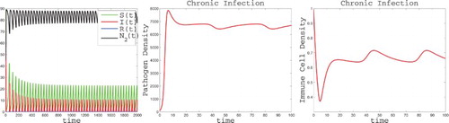
Motivated by the oscillations of the simple ODE immuno-eco-epidemiological model in Section 3, we searched for oscillations in model (1(1) $\begin{array}{rl}{V}_t(\tau ,t)+V_{\tau }(\tau ,t)& =r_{v}V(\tau ,t)(1-qV(\tau ,t\left)\right)-aV(\tau ,t)z(\tau ,t),\\ z_t(\tau ,t)+z_{\tau }(\tau ,t)& =\frac{b_{0}V(\tau ,t)z(\tau ,t)}{\left(p{N}_2\right(t)+D)(1+b_{2}V)}-\mu z(\tau ,t).\end{array}$(1) )–(4(4) $\begin{array}{rl}{S}^{\prime }& =r_1\left(1-\frac{N_1+{\alpha }_{12}{N}_2}{K_1}\right)N_1-S\left(t\right){\int }_0^{\mathrm{\infty }}\beta \left(\tau \right)i(\tau ,t)\mathrm{d}\tau -m_{1}S\left(t\right),\\ i_{\tau }(\tau ,t)+i_t(\tau ,t)& =-(m_1+\alpha (\tau )+\gamma (\tau \left)\right)i(\tau ,t),\\ i(0,t)& =S\left(t\right){\int }_0^{\mathrm{\infty }}\beta \left(\tau \right)i(\tau ,t)\mathrm{d}\tau ,\\ R^{\prime }& ={\int }_0^{\mathrm{\infty }}\gamma \left(\tau \right)i(\tau ,t)\mathrm{d}\tau -m_{1}R,\\ N_2^{\prime }\left(t\right)& =r_2\left(1-\frac{N_2+{\alpha }_{21}{N}_1}{K_2}\right)N_2-m_2{N}_2.\end{array}$(4) ). The presence of oscillations in the ODE model does not imply oscillations in the PDE model as the ODE model is not a special case of the PDE model. In single-scale time-since-infection structured models, the endemic equilibrium is usually destabilized by choosing a simple step function as the transmission rate. This cannot be done with multi-scale models where the transmission rate comes from the solution of the within-host model and is not arbitrary. Hence, in multi-scale models, a stabilization of the population-level equilibrium may occur [23]. If stabilization does not occur, showing loss of stability and oscillations is not a trivial task. The complexity of the characteristic equation and the implicit dependence on within-host parameters obstruct analysis for finding parameter values that give roots with positive real parts. We approached the problem numerically, and obtained oscillations for some parameter combinations such as those in Figure 7, although there is no guarantee that these are indeed sustained oscillations. To obtain the oscillations, we use α (or η) as a bifurcation parameter. Increasing α leads to oscillations. We were also able to produce oscillations in the case in which $\gamma \left(\tau \right)=0$ and ${\alpha }_{12}=0$ but $p\ne 0$, suggesting that the effect of species 2 on species 1's immunity plays the main role in the destabilization. The parameters that produce the oscillations in Figure 7 also give instability in the corresponding ODE model considered in Section 3. However, if $m_1$ is increased to 0.035, the ODE model is stable while the full model is unstable. The full model introduces a delay in the increase in V (and therefore β and α) relative to the ODE model, which tends to destabilize the system.

Figure 7. Oscillations in system (1(1) $\begin{array}{rl}{V}_t(\tau ,t)+V_{\tau }(\tau ,t)& =r_{v}V(\tau ,t)(1-qV(\tau ,t\left)\right)-aV(\tau ,t)z(\tau ,t),\\ z_t(\tau ,t)+z_{\tau }(\tau ,t)& =\frac{b_{0}V(\tau ,t)z(\tau ,t)}{\left(p{N}_2\right(t)+D)(1+b_{2}V)}-\mu z(\tau ,t).\end{array}$(1) )–(4(4) $\begin{array}{rl}{S}^{\prime }& =r_1\left(1-\frac{N_1+{\alpha }_{12}{N}_2}{K_1}\right)N_1-S\left(t\right){\int }_0^{\mathrm{\infty }}\beta \left(\tau \right)i(\tau ,t)\mathrm{d}\tau -m_{1}S\left(t\right),\\ i_{\tau }(\tau ,t)+i_t(\tau ,t)& =-(m_1+\alpha (\tau )+\gamma (\tau \left)\right)i(\tau ,t),\\ i(0,t)& =S\left(t\right){\int }_0^{\mathrm{\infty }}\beta \left(\tau \right)i(\tau ,t)\mathrm{d}\tau ,\\ R^{\prime }& ={\int }_0^{\mathrm{\infty }}\gamma \left(\tau \right)i(\tau ,t)\mathrm{d}\tau -m_{1}R,\\ N_2^{\prime }\left(t\right)& =r_2\left(1-\frac{N_2+{\alpha }_{21}{N}_1}{K_2}\right)N_2-m_2{N}_2.\end{array}$(4) ). Linking parameters are as version 2 in Table 3. Parameter values are: $r_1=0.1$, $\mu =0.25$, p=1, D=5, $m_1=0.01$, $m_2=0.1$, ${\alpha }_{12}=0$, ${\alpha }_{21}=0.5$, $K_1=100$, $b_0=0.005$, $\eta =0.001$, $r_2=1$, $K_2=100$, $\gamma \left(\tau \right)=0$, $r_v=2$, q=0.0001, a=1, $b_0=0.1$, $b_2=0.0002$, $V_0=100$, $z_0=1$, ${\beta }_0=0.2$, ${ϵ}_0=0.5$, B=1000.

6. Discussion

Understanding infectious disease ecology increasingly involves on one hand linking processes at different scales (in particular, within-host pathogen dynamics, and between-host transmission), and on the other embedding infectious disease processes in a broader community context, where species compete and are embedded in a wide range of food web interactions. In this article, we introduce a novel nested time-since-infection eco-epidemiological model of competition with a within-host model including an immune response in disease-affected species 1. Species 2 competes not only directly for resources with species 1 but also by affecting negatively species 1's immune response to the infection. We term this mode of competition stress-induced competition. The model involves bidirectional linkage of the within-host and between-host systems. This necessitates casting the within-host model in PDE form. We also present a related ODE model.

We find that stress-induced competition is capable of producing backward bifurcation with respect to the species 2 invasion number. Backward bifurcation of competitor invasion allows the competitor to persist alongside species 1 for values of its invasion number below one. In the age-structured case (the PDE model), we find that the backward bifurcation is very pronounced, allowing species 2 to persist alongside species 1 for values of its invasion number very close to zero. In the case of this backward bifurcation, two coexistence equilibria of species 1 and species 2 exist, and one equilibrium in which species 2 is not present. If species 2's invasion number is below one, species 2 may persist only in the case in which its initial numbers are sufficiently large.

Furthermore, we find that in the PDE case, the coexistence equilibrium of species 1 and species 2 may become destabilized and we sometimes observed numerically sustained oscillations. We show that the coexistence equilibrium is locally stable in the absence of disease-induced mortality or in the absence of recovery and competition (both interspecific and stress-induced) of species 2 with species 1. This destabilization occurs as a result of the disease-induced mortality and stress-induced competition of species 2 with species 1. Hence, the interplay of competition and pathogen dynamics can generate large-magnitude oscillations, when neither process on its own leads to instability (see Figure 5 and 7 for examples).

The age-structured immuno-eco-epidemiological model exhibits significant mathematical complexity. There can be alternative equilibria, with all species present at each equilibrium, for instance. In producing examples of the backward bifurcations and oscillations in the PDE model, we were guided by an appropriately designed three-dimensional ODE immuno-eco-epidemiological model, obtained under the assumption that the disease is chronic and within-host dynamics are fast. This simple ODE model is not a special case of the PDE model but exhibits both the backward bifurcation in the invasion number of species 2 and the oscillations we found in the PDE model. We surmise that specially designed simple ODE models may be used to study these types of complex systems and derive conclusions about their behavior.

Using the ODE model, we further observe that stress-induced competition leads to a lower number of susceptible individuals at equilibrium when the population of species 2 increases. In contrast, in the absence of stress-induced competition, species 2 numbers do not affect the number of susceptibles in the population of species 1. A more surprising result is that although single-scale eco-epidemiological models generally suggest that competition (and predation) lead to lower disease prevalence in the focal species, we find that stress-induced competition may increase the prevalence in species 1 when the population of species 2 is small. This occurs in a chronic disease without recovery. So stress-induced competition can enhance disease prevalence in a focal host species.

The interplay between within-host immune dynamics and ecological interactions is just beginning to be studied. There are many interesting questions yet to be addressed. Our observation that the dynamics of complex nested immuno-eco-epidemiological models can sometimes be obtained by a simple, related ODE model opens the door for further investigations and analysis. Our PDE and respective ODE models could be extended, for instance, so that the pathogen infects both hosts. This can add an immune dimension to apparent competition interactions and could lead to complex feedbacks. For instance, if species 2 weakens the immune response in species 1, and boosts disease prevalence in the latter, this could ‘spill back’ to boost disease levels in species 2. Another interesting avenue is to examine how the within-host immune dynamics affect predator–prey interactions. Two types of scenarios may be considered here: one with disease in the prey and the other with disease in the predator. Predation can alter immune responses, directly and negatively because prey experience stress or spend less time feeding, or indirectly because lower prey numbers boost resources available per prey, increasing resource acquisition rates and permitting stronger immune responses to infection. Coupling such responses with predator–prey and host–pathogen dynamics could potentially lead to complex dynamics. Likewise, also, immune responses in predators to their own pathogens may depend on how rapidly they can feed and garner resources to use in mounting such responses. We suggest that examining such effects of interspecific interactions on within-host pathogen dynamics, with consequent impacts on among-host disease transmission, provides a rich avenue for future theoretical and empirical investigations.

Acknowledgements

The authors thank Horst R. Thieme for valuable suggestions.

Disclosure statement

No potential conflict of interest was reported by the authors.

ORCID

Maia Martcheva http://orcid.org/0000-0001-8968-1663

Necibe Tuncer http://orcid.org/0000-0002-6388-2499

Robert D. Holt http://orcid.org/0000-0002-6685-547X

Additional information

Funding

This work was supported by the National Science Foundation [grant numbers DMS 1515661/1515442] and the University of Florida Foundation.

Appendix 1: Stability of ${\mathcal{E}}^{\ast }$

Proof.

The system for the perturbations in this case becomes: (A1) $\begin{array}{rl}\lambda s& =r_1\left(1-\frac{N_1^{\ast }}{K_1}\right)n_1-\frac{r_1}{K_1}(n_1+{\alpha }_{12}{n}_2)N_1^{\ast }-S^{\ast }{\int }_0^{\mathrm{\infty }}\beta \left(\tau \right)y\left(\tau \right)\mathrm{d}\tau \\ & -s{\int }_0^{\mathrm{\infty }}\beta \left(\tau \right)i^{\ast }\left(\tau \right)\mathrm{d}\tau -m_{1}s-n_2{S}^{\ast }{\int }_0^{\mathrm{\infty }}\frac{\mathrm{\partial }\beta \left(\tau \right)}{\mathrm{\partial }{N}_2}{i}^{\ast }\left(\tau \right)\mathrm{d}\tau ,\\ y_{\tau }\left(\tau \right)+\lambda y\left(\tau \right)& =-(m_1+\alpha (\tau )+\gamma (\tau \left)\right)y\left(\tau \right)-\left(\frac{\mathrm{\partial }\alpha \left(\tau \right)}{\mathrm{\partial }{N}_2}+\frac{\mathrm{\partial }\gamma \left(\tau \right)}{\mathrm{\partial }{N}_2}\right)i^{\ast }\left(\tau \right)n_2,\\ y\left(0\right)& =S^{\ast }{\int }_0^{\mathrm{\infty }}\beta \left(\tau \right)y\left(\tau \right)\mathrm{d}\tau +s{\int }_0^{\mathrm{\infty }}\beta \left(\tau \right)i^{\ast }\left(\tau \right)\mathrm{d}\tau +n_2{S}^{\ast }{\int }_0^{\mathrm{\infty }}\frac{\mathrm{\partial }\beta \left(\tau \right)}{\mathrm{\partial }{N}_2}{i}^{\ast }\left(\tau \right)\mathrm{d}\tau ,\\ \lambda r& ={\int }_0^{\mathrm{\infty }}\gamma \left(\tau \right)y\left(\tau \right)\mathrm{d}\tau -m_{1}r+n_2{\int }_0^{\mathrm{\infty }}\frac{\mathrm{\partial }\gamma \left(\tau \right)}{\mathrm{\partial }{N}_2}{i}^{\ast }\left(\tau \right)\mathrm{d}\tau ,\\ \lambda n_2& =r_2\left(1-\frac{{\alpha }_{21}{N}_1^{\ast }}{K_2}\right)n_2-m_2{n}_2.\end{array}$(A1) The first eigenvalue is ${\lambda }_1=r_2(1-{\alpha }_{21}{N}_1^{\ast }/K_2)-m_2<0$ if and only if ${\hat{\mathcal{R}}}_2<1$. Hence if ${\hat{\mathcal{R}}}_2>1$, equilibrium ${\mathcal{E}}^{\ast }$ is unstable. If ${\hat{\mathcal{R}}}_2<1$ the stability of ${\mathcal{E}}^{\ast }$ depends on the eigenvalues of the remaining system: (A2) $\begin{array}{rl}\lambda s& =\sigma n_1-S^{\ast }{\int }_0^{\mathrm{\infty }}\beta \left(\tau \right)y\left(\tau \right)\mathrm{d}\tau -Bs-m_{1}s\\ y_{\tau }\left(\tau \right)+\lambda y\left(\tau \right)& =-(m_1+\alpha (\tau )+\gamma (\tau \left)\right)y\left(\tau \right),\\ y\left(0\right)& =S^{\ast }{\int }_0^{\mathrm{\infty }}\beta \left(\tau \right)y\left(\tau \right)\mathrm{d}\tau +Bs,\\ \lambda r& ={\int }_0^{\mathrm{\infty }}\gamma \left(\tau \right)y\left(\tau \right)\mathrm{d}\tau -m_{1}r.\end{array}$(A2)

where $\sigma =r_1(1-2N_1^{\ast }/K_1)$ and $B={\int }_0^{\mathrm{\infty }}\beta \left(\tau \right)i^{\ast }\left(\tau \right)\mathrm{d}\tau .$

Case 1: First, we assume that the disease leads to no recovery, that is $\gamma \left(\tau \right)=0$. Assume also $0<\sigma <m_1$.

Solving the differential equation and substituting in the other equations, we have (A3) $\begin{array}{rl}\lambda s& =\sigma n_1-m_{1}s-y\left(0\right),\\ y\left(0\right)& =S^{\ast }y\left(0\right){\int }_0^{\mathrm{\infty }}\beta \left(\theta \right)\pi \left(\theta \right){\mathrm{e}}^{-\lambda \theta }\mathrm{d}\theta +Bs,\\ n_1& =s+y\left(0\right)\rho \left(\lambda \right)+r,\\ r& =y\left(0\right)\mathrm{\Gamma }\left(\lambda \right),\end{array}$(A3) where (A4) $\mathrm{\Gamma }\left(\lambda \right)=\frac{{\int }_0^{\mathrm{\infty }}\gamma \left(\tau \right)\pi \left(\tau \right){\mathrm{e}}^{-\lambda \tau }\mathrm{d}\tau }{\lambda +m_1}\rho \left(\lambda \right)={\int }_0^{\mathrm{\infty }}\pi \left(\tau \right){\mathrm{e}}^{-\lambda \tau }\mathrm{d}\tau .$(A4) Replacing r in the third equation, we obtain (A5) $\begin{array}{rl}\lambda s& =\sigma n_1-m_{1}s-y\left(0\right),\\ y\left(0\right)& =S^{\ast }y\left(0\right){\int }_0^{\mathrm{\infty }}\beta \left(\theta \right)\pi \left(\theta \right){\mathrm{e}}^{-\lambda \theta }\mathrm{d}\theta +Bs,\\ n_1& =s+y\left(0\right)\left(\rho \right(\lambda )+\mathrm{\Gamma }(\lambda \left)\right).\end{array}$(A5) Replacing $n_1$ from the last equation into the first equation and solving for s, we obtain (A6) $s=\frac{-y\left(0\right)(1-\sigma \rho (\lambda )-\sigma \mathrm{\Gamma }(\lambda \left)\right)}{\lambda +m_1-\sigma }.$(A6) Substituting s into the initial condition and canceling $y\left(0\right),$ we obtain the following characteristic equation for λ: (A7) $1+B\frac{(1-\sigma \rho (\lambda )-\sigma \mathrm{\Gamma }(\lambda \left)\right)}{\lambda +m_1-\sigma }=S^{\ast }{\int }_0^{\mathrm{\infty }}\beta \left(\theta \right)\pi \left(\theta \right){\mathrm{e}}^{-\lambda \theta }\mathrm{d}\theta .$(A7) Denote by $\mathcal{L}\left(\lambda \right)$ the left-hand side of the equation above and by $\mathcal{H}\left(\lambda \right)$, the right-hand side. Next, we show that if $\sigma <m_1$ the characteristic equation (A7(A7) $1+B\frac{(1-\sigma \rho (\lambda )-\sigma \mathrm{\Gamma }(\lambda \left)\right)}{\lambda +m_1-\sigma }=S^{\ast }{\int }_0^{\mathrm{\infty }}\beta \left(\theta \right)\pi \left(\theta \right){\mathrm{e}}^{-\lambda \theta }\mathrm{d}\theta .$(A7) ) does not have a real positive root. In this case, both sides of Equation (A7(A7) $1+B\frac{(1-\sigma \rho (\lambda )-\sigma \mathrm{\Gamma }(\lambda \left)\right)}{\lambda +m_1-\sigma }=S^{\ast }{\int }_0^{\mathrm{\infty }}\beta \left(\theta \right)\pi \left(\theta \right){\mathrm{e}}^{-\lambda \theta }\mathrm{d}\theta .$(A7) ) are defined for all real and positive λ, and, (A8) $1+B\frac{(1-\sigma \rho (\lambda )-\sigma \mathrm{\Gamma }(\lambda \left)\right)}{\lambda +m_1-\sigma }>1+B\frac{(1-\sigma \rho (0)-\sigma \mathrm{\Gamma }(0\left)\right)}{\lambda +m_1-\sigma }>1.$(A8) This last inequality follows from the fact that $1-\sigma \rho \left(0\right)-\sigma \mathrm{\Gamma }\left(0\right)>0.$ On the other hand, $S^{\ast }{\int }_0^{\mathrm{\infty }}\beta \left(\theta \right)\pi \left(\theta \right){\mathrm{e}}^{-\lambda \theta }\mathrm{d}\theta <S^{\ast }{\int }_0^{\mathrm{\infty }}\beta \left(\theta \right)\pi \left(\theta \right)\mathrm{d}\theta =1.$ Now, we show that if $\gamma \left(\tau \right)=0$ and $0<\sigma <m_1$, then ${\mathcal{E}}^{\ast }$ is locally asymptotically stable. This result is analogous to the result in [2]. Since the characteristic equation cannot have real non-negative roots, we then show that the characteristic equation (A7(A7) $1+B\frac{(1-\sigma \rho (\lambda )-\sigma \mathrm{\Gamma }(\lambda \left)\right)}{\lambda +m_1-\sigma }=S^{\ast }{\int }_0^{\mathrm{\infty }}\beta \left(\theta \right)\pi \left(\theta \right){\mathrm{e}}^{-\lambda \theta }\mathrm{d}\theta .$(A7) ) cannot have purely imaginary roots. To see that, we take $\lambda =\eta i$. Then (A9) $\begin{array}{rl}{S}^{\ast }{\int }_0^{\mathrm{\infty }}\beta \left(\tau \right)\pi \left(\tau \right){\mathrm{e}}^{-i\eta \tau }\mathrm{d}\tau & =S^{\ast }{\int }_0^{\mathrm{\infty }}\beta \left(\tau \right)\pi \left(\tau \right)\cos \left(\eta \tau \right)\mathrm{d}\tau -i{S}^{\ast }{\int }_0^{\mathrm{\infty }}\beta \left(\tau \right)\pi \left(\tau \right)\sin \left(\eta \tau \right)\mathrm{d}\tau \\ & =1+B\frac{(1-\sigma \mathrm{\Re }\rho -\sigma \mathrm{\Re \Gamma }+i\sigma \mathrm{\Im }\rho +i\sigma \mathrm{\Im \Gamma })(m_1-\sigma -i\eta )}{(m_1-\sigma {)}^2+{\eta }^2}\end{array}$(A9) Equating the real and the imaginary parts, we have the following system: (A10) $\begin{array}{rl}& 1+B\frac{(1-\sigma \mathrm{\Re }\rho -\sigma \mathrm{\Re \Gamma })(m_1-\sigma )-\eta (\sigma \mathrm{\Im }\rho +\sigma \mathrm{\Im \Gamma })}{(m_1-\sigma {)}^2+{\eta }^2}\\ & =S^{\ast }{\int }_0^{\mathrm{\infty }}\beta \left(\tau \right)\pi \left(\tau \right)\cos \left(\eta \tau \right)\mathrm{d}\tau ,\\ & B\frac{(1-\sigma \mathrm{\Re }\rho -\sigma \mathrm{\Re \Gamma })y+(m_1-\sigma )(\sigma \mathrm{\Im }\rho +\sigma \mathrm{\Im \Gamma })}{(m_1-\sigma {)}^2+{\eta }^2}\\ & =S^{\ast }{\int }_0^{\mathrm{\infty }}\beta \left(\tau \right)\pi \left(\tau \right)\sin \left(\eta \tau \right)\mathrm{d}\tau ,\end{array}$(A10) where (A11) $\begin{array}{rl}\mathrm{\Re \Gamma }& =\frac{{\int }_0^{\mathrm{\infty }}\gamma \left(\tau \right)\pi \left(\tau \right)\cos \left(y\tau \right)\mathrm{d}\tau \left(m_1\right)-y{\int }_0^{\mathrm{\infty }}\gamma \left(\tau \right)\pi \left(\tau \right)\sin \left(y\tau \right)\mathrm{d}\tau }{(m_1{)}^2+y^2},\\ \mathrm{\Im \Gamma }& =-\frac{{\int }_0^{\mathrm{\infty }}\gamma \left(\tau \right)\pi \left(\tau \right)\sin \left(y\tau \right)\mathrm{d}\tau \left(m_1\right)+y{\int }_0^{\mathrm{\infty }}\gamma \left(\tau \right)\pi \left(\tau \right)\cos \left(y\tau \right)\mathrm{d}\tau }{(m_1{)}^2+{\eta }^2},\\ \mathrm{\Re }\rho & ={\int }_0^{\mathrm{\infty }}\pi \left(\tau \right)\cos \left(\eta \tau \right)\mathrm{d}\tau ,\\ \mathrm{\Im }\rho & =-{\int }_0^{\mathrm{\infty }}\pi \left(\tau \right)\sin \left(\eta \tau \right)\mathrm{d}\tau .\end{array}$(A11)

First, we notice that $1-\sigma \mathrm{\Re }\rho -\sigma \mathrm{\Re \Gamma }>1-\sigma \mathrm{\Pi }>0$. Then, we notice that $-\mathrm{\Im }\rho >0$. Hence with $\gamma \left(\tau \right)=0$ and $\sigma >0$, we have that $B\frac{(1-\sigma \mathrm{\Re }\rho -\sigma \mathrm{\Re \Gamma }+i\sigma \mathrm{\Im }\rho +i\sigma \mathrm{\Im \Gamma })(m_1-\sigma -i\eta )}{(m_1-\sigma {)}^2+{\eta }^2}>0$ and the left-hand side in the first equation in Equation (A10(A10) $\begin{array}{rl}& 1+B\frac{(1-\sigma \mathrm{\Re }\rho -\sigma \mathrm{\Re \Gamma })(m_1-\sigma )-\eta (\sigma \mathrm{\Im }\rho +\sigma \mathrm{\Im \Gamma })}{(m_1-\sigma {)}^2+{\eta }^2}\\ & =S^{\ast }{\int }_0^{\mathrm{\infty }}\beta \left(\tau \right)\pi \left(\tau \right)\cos \left(\eta \tau \right)\mathrm{d}\tau ,\\ & B\frac{(1-\sigma \mathrm{\Re }\rho -\sigma \mathrm{\Re \Gamma })y+(m_1-\sigma )(\sigma \mathrm{\Im }\rho +\sigma \mathrm{\Im \Gamma })}{(m_1-\sigma {)}^2+{\eta }^2}\\ & =S^{\ast }{\int }_0^{\mathrm{\infty }}\beta \left(\tau \right)\pi \left(\tau \right)\sin \left(\eta \tau \right)\mathrm{d}\tau ,\end{array}$(A10) ) is bigger than one. On the other hand, the right-hand side is smaller or equal to one. Hence, there is no y>0 that satisfies that equation. Hence in this case, the characteristic equation has roots with only negative real parts, and ${\mathcal{E}}^{\ast }$ is locally asymptotically stable.

Case 2: Assume the disease is non-fatal, $\alpha \left(\tau \right)=0$.

Integrating the second equation in system (A2(A2) $\begin{array}{rl}\lambda s& =\sigma n_1-S^{\ast }{\int }_0^{\mathrm{\infty }}\beta \left(\tau \right)y\left(\tau \right)\mathrm{d}\tau -Bs-m_{1}s\\ y_{\tau }\left(\tau \right)+\lambda y\left(\tau \right)& =-(m_1+\alpha (\tau )+\gamma (\tau \left)\right)y\left(\tau \right),\\ y\left(0\right)& =S^{\ast }{\int }_0^{\mathrm{\infty }}\beta \left(\tau \right)y\left(\tau \right)\mathrm{d}\tau +Bs,\\ \lambda r& ={\int }_0^{\mathrm{\infty }}\gamma \left(\tau \right)y\left(\tau \right)\mathrm{d}\tau -m_{1}r.\end{array}$(A2) ) and adding the equations in Equation (A2(A2) $\begin{array}{rl}\lambda s& =\sigma n_1-S^{\ast }{\int }_0^{\mathrm{\infty }}\beta \left(\tau \right)y\left(\tau \right)\mathrm{d}\tau -Bs-m_{1}s\\ y_{\tau }\left(\tau \right)+\lambda y\left(\tau \right)& =-(m_1+\alpha (\tau )+\gamma (\tau \left)\right)y\left(\tau \right),\\ y\left(0\right)& =S^{\ast }{\int }_0^{\mathrm{\infty }}\beta \left(\tau \right)y\left(\tau \right)\mathrm{d}\tau +Bs,\\ \lambda r& ={\int }_0^{\mathrm{\infty }}\gamma \left(\tau \right)y\left(\tau \right)\mathrm{d}\tau -m_{1}r.\end{array}$(A2) ), we obtain the equation of the total population size: $(\lambda +m_1-\sigma )n_1=0.$ From here it follows that ${\lambda }_1=\sigma -m_1$. Thus if $\sigma -m_1<0$ the stability of the system depends on the remaining eigenvalues. If $\sigma >m_1$ the equilibrium is unstable. Assume $\sigma -m_1<0$, then the stability of ${\mathcal{E}}^{\ast }$ depends on the eigenvalues of the system (A12) $\begin{array}{rl}\lambda s& =-m_{1}s-y\left(0\right),\\ y\left(0\right)& =S^{\ast }y\left(0\right){\int }_0^{\mathrm{\infty }}\beta \left(\theta \right)\pi \left(\theta \right){\mathrm{e}}^{-\lambda \theta }\mathrm{d}\theta +Bs,\\ \lambda r& =y\left(0\right)\hat{\mathrm{\Gamma }}\left(\lambda \right)-m_{1}r,\end{array}$(A12) where $\hat{\mathrm{\Gamma }}\left(\lambda \right)={\int }_0^{\mathrm{\infty }}\gamma \left(\tau \right)\pi \left(\tau \right){\mathrm{e}}^{-\lambda \tau }\mathrm{d}\tau$. Adding the equations for s and r, we have $s+r=\frac{-y\left(0\right)[1-\hat{\mathrm{\Gamma }}(\lambda \left)\right]}{\lambda +m_1}.$ Since $r=\frac{y\left(0\right)\hat{\mathrm{\Gamma }}\left(\lambda \right)}{\lambda +m_1}$ and s=s+r−r, we have that $s=\frac{-y\left(0\right)}{(\lambda +m_1)}.$

The characteristic equation becomes: (A13) $(\lambda +m_1+B)/(\lambda +m_1)=S^{\ast }{\int }_0^{\mathrm{\infty }}\beta \left(\tau \right)\pi \left(\tau \right){\mathrm{e}}^{-\lambda \tau }\mathrm{d}\tau .$(A13) The left-hand side of this equation is $(\lambda +m_1+B)/(\lambda +m_1)$. The absolute value of this expression for λ with non-negative real part is greater than one. On the other hand, the absolute value of the right-hand side satisfies: $\left|S^{\ast }{\int }_0^{\mathrm{\infty }}\beta \left(\tau \right)\pi \left(\tau \right){\mathrm{e}}^{-\lambda \tau }\mathrm{d}\tau \right|\le S^{\ast }{\int }_0^{\mathrm{\infty }}\beta \left(\tau \right)\pi \left(\tau \right)\mathrm{d}\tau =1.$ Hence, there are no solutions with non-negative real part and ${\mathcal{E}}^{\ast }$ is locally asymptotically stable. This completes the proof.

Appendix 2. Proof of stability of coexistence equilibrium

Proof.

When p=0 all derivatives of β, α and γ with respect to $N_2$ are zero. When $\alpha \left(\tau \right)=0$, the equation for $n_1$ becomes $(\lambda -{\sigma }_1+m_1)n_1=0$. Hence, if $\lambda \ne {\sigma }_1-m_1$, $n_1=0$. From the last equation of Equation (32(32) $\begin{array}{rl}{s}^{\prime }& =r_1\left(1-\frac{N_1^{\ast }+{\alpha }_{12}{N}_2^{\ast }}{K_1}\right)n_1-\frac{r_1}{K_1}(n_1+{\alpha }_{12}{n}_2)N_1^{\ast }\\ & -S^{\ast }{\int }_0^{\mathrm{\infty }}\beta \left(\tau \right)y(\tau ,t)\mathrm{d}\tau -s\left(t\right){\int }_0^{\mathrm{\infty }}\beta \left(\tau \right)i^{\ast }\left(\tau \right)\mathrm{d}\tau -m_{1}s\left(t\right)\\ & -n_2\left(t\right)S^{\ast }{\int }_0^{\mathrm{\infty }}\frac{\mathrm{\partial }\beta \left(\tau \right)}{\mathrm{\partial }{N}_2}{i}^{\ast }\left(\tau \right)\mathrm{d}\tau ,\\ y_{\tau }(\tau ,t)+y_t(\tau ,t)& =-(m_1+\alpha (\tau )+\gamma (\tau \left)\right)y(\tau ,t)\\ & -\left(\frac{\mathrm{\partial }\alpha \left(\tau \right)}{\mathrm{\partial }{N}_2}{i}^{\ast }\left(\tau \right)+\frac{\mathrm{\partial }\gamma \left(\tau \right)}{\mathrm{\partial }{N}_2}{i}^{\ast }\left(\tau \right)\right)n_2\left(t\right)\\ & -\left(\frac{\mathrm{\partial }\alpha \left(\tau \right)}{\mathrm{\partial }V}{i}^{\ast }\left(\tau \right)+\frac{\mathrm{\partial }\gamma \left(\tau \right)}{\mathrm{\partial }V}{i}^{\ast }\left(\tau \right)\right)u(\tau ,t)\\ & -\left(\frac{\mathrm{\partial }\alpha \left(\tau \right)}{\mathrm{\partial }z}{i}^{\ast }\left(\tau \right)+\frac{\mathrm{\partial }\gamma \left(\tau \right)}{\mathrm{\partial }z}{i}^{\ast }\left(\tau \right)\right)w(\tau ,t),\\ y(0,t)& =S^{\ast }{\int }_0^{\mathrm{\infty }}\beta \left(\tau \right)y(\tau ,t)\mathrm{d}\tau +s\left(t\right){\int }_0^{\mathrm{\infty }}\beta \left(\tau \right)i^{\ast }\left(\tau \right)\mathrm{d}\tau \\ & +n_2\left(t\right)S^{\ast }{\int }_0^{\mathrm{\infty }}\frac{\mathrm{\partial }\beta \left(\tau \right)}{\mathrm{\partial }{N}_2}{i}^{\ast }\left(\tau \right)\mathrm{d}\tau ,\\ r^{\prime }& ={\int }_0^{\mathrm{\infty }}\gamma \left(\tau \right)y(\tau ,t)\mathrm{d}\tau -m_{1}r+{\int }_0^{\mathrm{\infty }}\frac{\mathrm{\partial }\gamma \left(\tau \right)}{\mathrm{\partial }{N}_2}{i}^{\ast }\left(\tau \right)\mathrm{d}\tau n_2\left(t\right),\\ n_2^{\prime }\left(t\right)& =r_2\left(1-\frac{N_2^{\ast }+{\alpha }_{21}{N}_1^{\ast }}{K_2}\right)n_2-\frac{r_2}{K_2}(n_2+{\alpha }_{21}{n}_1)N_2^{\ast }-m_2{n}_2.\end{array}$(32) ), we have another eigenvalue $\lambda =-r_2{N}_2^{\ast \ast }/K_2$ or $n_2=0$. Thus again, all terms with the derivatives of β, α and γ with respect to $N_2$ are zero. This simplifies the system for the perturbations significantly. Using the equations for the coexistence equilibrium, the system for the perturbations takes the form: (A14) $\begin{array}{rl}\lambda s& =r_1\left(1-\frac{N_1^{\ast \ast }+{\alpha }_{12}{N}_2^{\ast \ast }}{K_1}\right)n_1-\frac{r_1}{K_1}(n_1+{\alpha }_{12}{n}_2)N_1^{\ast \ast }\\ & -S^{\ast }{\int }_0^{\mathrm{\infty }}\beta \left(\tau \right)y\left(\tau \right)\mathrm{d}\tau -Bs-m_{1}s,\\ y_{\tau }\left(\tau \right)+\lambda y\left(\tau \right)& =-(m_1+\alpha (\tau )+\gamma (\tau \left)\right)y\left(\tau \right),\\ y\left(0\right)& =S^{\ast }{\int }_0^{\mathrm{\infty }}\beta \left(\tau \right)y\left(\tau \right)\mathrm{d}\tau +Bs,\\ \lambda r& ={\int }_0^{\mathrm{\infty }}\gamma \left(\tau \right)y\left(\tau \right)\mathrm{d}\tau -m_{1}r,\\ \lambda n_2& =-\frac{r_2}{K_2}(n_2+{\alpha }_{21}{n}_1)N_2^{\ast \ast },\end{array}$(A14) where $B={\int }_0^{\mathrm{\infty }}\beta \left(\tau \right)i^{\ast }\left(\tau \right)\mathrm{d}\tau$. From the last equation, we express $n_2$ in terms of $n_1$: (A15) $n_2=-D\left(\lambda \right)n_1,$(A15) where $D\left(\lambda \right)=\frac{{\alpha }_{21}\frac{r_2}{K_2}{N}_2^{\ast \ast }}{\lambda +\frac{r_2}{K_2}{N}_2^{\ast \ast }}.$ Furthermore, as before, $r=y\left(0\right)\mathrm{\Gamma }\left(\lambda \right).$ Substituting $n_2$ and r in the first three equations, we obtain (A16) $\begin{array}{rl}\lambda s& =({\sigma }_1+D_1(\lambda \left)\right)n_1-S^{\ast }{\int }_0^{\mathrm{\infty }}\beta \left(\tau \right)y\left(\tau \right)\mathrm{d}\tau -Bs-m_{1}s,\\ y_{\tau }\left(\tau \right)+\lambda y\left(\tau \right)& =-(m_1+\alpha (\tau )+\gamma (\tau \left)\right)y\left(\tau \right),\\ y\left(0\right)& =S^{\ast }{\int }_0^{\mathrm{\infty }}\beta \left(\tau \right)y\left(\tau \right)\mathrm{d}\tau +Bs,\end{array}$(A16) where $D_1\left(\lambda \right)=\left(r_1{N}_1^{\ast \ast }/K_1\right){\alpha }_{12}D\left(\lambda \right)$. Solving the differential equation and substituting $y\left(\tau \right)$, and using the boundary condition, we can express s in terms of $y\left(0\right)$: (A17) $s=-\frac{1-({\sigma }_1+D_1(\lambda \left)\right)\rho \left(\lambda \right)-({\sigma }_1+D_1(\lambda \left)\right)\mathrm{\Gamma }\left(\lambda \right)}{\lambda +m_1-{\sigma }_1-D_1\left(\lambda \right)}y\left(0\right).$(A17) Substituting this into the equation for the initial condition and canceling $y\left(0\right)$, we obtain the characteristic equation of the coexistence equilibrium (A18) $1+B\frac{1-({\sigma }_1+D_1(\lambda \left)\right)\rho \left(\lambda \right)-({\sigma }_1+D_1(\lambda \left)\right)\mathrm{\Gamma }\left(\lambda \right)}{\lambda +m_1-{\sigma }_1-D_1\left(\lambda \right)}=S^{\ast }{\int }_0^{\mathrm{\infty }}\beta \left(\tau \right)\pi \left(\tau \right){\mathrm{e}}^{-\lambda \tau }\mathrm{d}\tau .$(A18)

First we show that if ${\sigma }_1+D_1\left(0\right)<m_1$, then the characteristic equation of the coexistence equilibrium does not have real non-negative roots. Denote by $\mathcal{L}\left(\lambda \right)$ the left-hand side of Equation (A18(A18) $1+B\frac{1-({\sigma }_1+D_1(\lambda \left)\right)\rho \left(\lambda \right)-({\sigma }_1+D_1(\lambda \left)\right)\mathrm{\Gamma }\left(\lambda \right)}{\lambda +m_1-{\sigma }_1-D_1\left(\lambda \right)}=S^{\ast }{\int }_0^{\mathrm{\infty }}\beta \left(\tau \right)\pi \left(\tau \right){\mathrm{e}}^{-\lambda \tau }\mathrm{d}\tau .$(A18) ) and by $\mathcal{H}\left(\lambda \right)$ – the right-hand side. For λ real and non-negative $\mathcal{H}\left(0\right)=1$ and $\underset{\lambda \to \mathrm{\infty }}{lim}\mathcal{H}\left(\lambda \right)=0$. Next, we show that $\mathcal{L}\left(0\right)>1$. To show that, we first notice that differentiating equation (28(28) $r_1\left(1-\frac{(1-{\alpha }_{12}{\alpha }_{21})N_1^{\ast \ast }+{\alpha }_{12}{K}_2(1-{\displaystyle \frac{m_2}{r_2})}}{K_1}\right)N_1^{\ast \ast }=\frac{N_1^{\ast \ast }-S^{\ast \ast }}{\mathrm{\Pi }+\mathrm{\Gamma }}+m_1{S}^{\ast \ast }.$(28) ) with respect to $N_1$ we have ${\sigma }_1+D_1\left(0\right)<\frac{1}{\mathrm{\Pi }+\gamma }.$ Hence, $\mathcal{L}\left(0\right)>1$. Furthermore, the numerator and the denominator in $\mathcal{L}\left(\lambda \right)$ remain positive for all real positive λ. Hence, $\mathcal{L}\left(\lambda \right)>1$ for all non-negative λ. On the other hand, $\mathcal{H}\left(\lambda \right)\le 1$ for all non-negative λ. So, the characteristic equation does not have real non-negative roots.

The local asymptotic stability of the coexistence equilibrium in the two cases can be established as the local stability of ${\mathcal{E}}^{\ast }$.

References

- R.M. Anderson and R.M. May, Infectious Diseases of Humans: Dynamics and Control, Oxford University Press, Oxford, 1991.
- S. Bhattacharya and M. Martcheva, An immuno-eco-epidemiological model of competition, J. Biol. Dyn. 10 (2016), pp. 314–341. doi: 10.1080/17513758.2016.1186291
- S. Bhattacharya, M. Martcheva, and X.Z. Li, A predator prey disease model with immune response in infected prey, J. Math. Anal. Appl. 411(1) (2014), pp. 297–313. doi: 10.1016/j.jmaa.2013.09.031
- E.T. Borer, A.L. Laine, and E.W. Seabloom, A multiscale approach to plant disease using the metacommunity concept, Annu. Rev. Phytopathol. 54 (2016), pp. 397–418. doi: 10.1146/annurev-phyto-080615-095959
- M.G. Buhnerkempe, M.G. Roberts, A.P. Dobson, H. Heesterbeek, P.J. Hudson, and J.O. LloydSmith, Eight challenges in modelling disease ecology in multihost, multiagent systems, Epidemics 10 (2015), pp. 26–30. doi: 10.1016/j.epidem.2014.10.001
- R.K. Chandra, Nutrition and the immune system: an introduction, Am. J. Clin. Nutr. 66 (1997), pp. 460–463.
- T. Day, S. Alizon, and N. Mideo, Bridging scales in the evolution of infectious disease life histories: theory, Evolution 65 (2011), pp. 3448–3461. doi: 10.1111/j.1558-5646.2011.01394.x
- Z. Feng, J. Velasco-Hernandez, and B. Tapia-Santos, A mathematical model for coupling within-host and between-host dynamics in an environmentally-driven infectious disease, Math. Biosci. 241(1) (2013), pp. 49–55. doi: 10.1016/j.mbs.2012.09.004
- Z. Feng, J. Velasco-Hernandez, B. Tapia-Santos, and M. Leite, A model for coupling within-host and between-host dynamics in an infectious disease, Nonlinear Dyn. 68 (2012), pp. 401–411. doi: 10.1007/s11071-011-0291-0
- M.A. Gilchrist and A. Sasaki, Modeling host-parasite coevolution: a nested approach based on mechanistic models, J. Theor. Biol. 218 (2002), pp. 289–308. doi: 10.1006/jtbi.2002.3076
- S.R. Hall, C.J. Knight, C.R. Becker, M.A. Duffy, A.J. Tessier, and C.E. Caceres, Quality matters: resource quality for hosts and the timing of epidemics, Ecol. Lett. 12 (2009), pp. 118–128. doi: 10.1111/j.1461-0248.2008.01264.x
- M.J. Hatcher and A.M. Dunn, Parasites in Ecological Communities: From Interactions to Ecosystems, Cambridge University Press, Cambridge, 2011.
- R.D. Holt, A biogeographical and landscape perspective on within-host infection dynamics, in Proceedings of the 8th International Symposium of Microbial Ecology, C.R. Bell, M. Brylinsky, and P. Johnson-Green, eds., Atlantic Canada Society for Microbial Ecology, Halifax, 2000, pp. 583–588.
- R.D. Holt and M. Barfield, Within-host pathogen dynamics: some ecological and evolutionary consequences of transients, dispersal mode, and within-host spatial heterogeneity, in Disease Evolution: Models, Concepts, and Data Analyses, Z. Feng, U. Dieckmann, and S. Levin, eds., American Mathematical Society, Providence, RI, 2006, pp. 45–66.
- R.D. Holt and A.P. Dobson, Extending the principles of community ecology to address the epidemiology of host-pathogen communities, in Disease Ecology: Community Structure and Invasion Pathogen Dynamics, S.K. Collinge and C. Ray, eds., Oxford University Press, Oxford, pp. 6–27, 2006.
- R.D. Holt, A.P. Dobson, M. Begon, R.G. Bowers, and E.M. Schauber, Parasite establishment in host communities, Ecol. Lett. 6 (2003), pp. 837–842. doi: 10.1046/j.1461-0248.2003.00501.x
- R.D. Holt and M. Roy, Predation can increase the prevalence of infectious disease, Am. Nat. 169 (2007), pp. 690–699. doi: 10.1086/513188
- M.J. Keeling and P. Rohani, Modelling Infectious Diseases in Humans and Animals, Princeton University Press, Princeton, NJ, 2008.
- M. Martcheva, Evolutionary consequences of predation for pathogens in prey, Bull. Math. Biol. 71(4) (2009), pp. 819–844. doi: 10.1007/s11538-008-9383-5
- M. Martcheva, An Immuno-epidemiological model of paratuberculosis, AIP Conf. Proc. 1404 (2011), pp. 176–183. doi: 10.1063/1.3659918
- M. Martcheva, An Introduction to Mathematical Epidemiology, Springer, New York, 2015.
- M. Martcheva, S. Lenhart, S. Eda, D. Klinkenberg, E. Momotani, and J. Stable, An immuno-epidemiological model for Johne's disease in cattle, Vet. Res. 46 (2015), article 69. doi: 10.1186/s13567-015-0190-3
- M. Martcheva and X.Z. Li, Linking immunological and epidemiological dynamics of HIV: the case of super-infection, J. Biol. Dyn. 7(1) (2013), pp. 161–182. doi: 10.1080/17513758.2013.820358
- M. Martcheva and H.R. Thieme, Progression age enhanced backward bifurcation in an epidemic model with super-infection, J. Math. Biol. 46(5) (2003), pp. 385–424. doi: 10.1007/s00285-002-0181-7
- M. Martcheva, N. Tuncer, and C.St. Mary, Coupling the within-host and between-host infectious disease modeling, Biomath 4(2) (2015), p. 201510091. doi: 10.11145/j.biomath.2015.10.091
- N. Mideo, S. Alizon, and T. Day, Linking within and between host dynamics in the evolutionary epidemiology of infectious diseases, Trends Ecol. Evol. 23 (2008), pp. 511–517. doi: 10.1016/j.tree.2008.05.009
- R.S. Ostfeld, F. Keesing, and V.T. Eviner, The ecology of infectious diseases: progress, challenges, and frontiers, in Infectious Disease Ecology: Effects of Ecosystems on Disease and of Disease on Ecosystems, R.S. Ostfeld, F. Keesing, and V. Eviner, eds., Princeton University Press, Princeton, NJ, 2008, pp. 469–482.
- D.A. Padgett and R. Glaser, How stress influences the immune response, Trends Immunol. 24 (2003), pp. 444–448. doi: 10.1016/S1471-4906(03)00173-X
- B. Roche, A.P. Dobson, J.F. Guegan, and P. Rohani, Linking community and disease ecology: the impact of biodiversity on pathogen transmission, Phil. Trans. Roy. Soc. 367 (2012), pp. 2807–2813. doi: 10.1098/rstb.2011.0364
- P. Schmid-Hempel, Evolutionary Parasitology: The Integrated Study of Infections, Immunology, Ecology and Genetics, Oxford University Press, Oxford, UK, 2011.
- E.W. Seabloom, E.T. Borer, K. Gross, A.E. Kendig, C. Lacroix, C.E. Mitchell, E.A. Mordecai, and A.G. Power, The community ecology of pathogens: coinfection, coexistence and community composition, Ecol. Lett. 18 (2015), pp. 410–415. doi: 10.1111/ele.12418
- V.H. Smith, Host resource supplies influence the dynamics and outcome of infectious disease: an ecological view, Integr. Comp. Biol. 47 (2007), pp. 310–316. doi: 10.1093/icb/icm006
- V.H. Smith, R.D. Holt, M.S. Smith, Y. Niu, and M. Barfield, Resources, mortality, and disease ecology: importance of positive feedbacks between host growth rate and pathogen dynamics, Israel J. Ecol. Evol. 61 (2015), pp. 37–49. doi: 10.1080/15659801.2015.1035508
- A.T. Strauss, M.S. Shocket, D.J. Civitello, J.L. Hite, R.M. Pencyzkowki, M.A. Duffy, C.E. Caceres, and S.R. Hall, Habitat, predators, and hosts regulate disease in Daphnia through direct and indirect pathways, Ecol. Monogr. 86 (2016), pp. 393–411. doi: 10.1002/ecm.1222
- D. Stiefs, E. Venturino, and U. Feudel, Evidence of chaos in eco-epidemic models, Math. Biosci. Eng. 6 (2009), pp. 855–871. doi: 10.3934/mbe.2009.6.855
- N. Tuncer, H. Gulbudak, V.L. Cannataro, and M. Martcheva, Structural and practical identifiability issues of immuno-epidemiological vector-host models with application to Rift Valley Fever, Bull. Math. Biol. 78 (2016), pp. 1796–1827. doi: 10.1007/s11538-016-0200-2
- P. van den Driessche and M.L. Zeeman, Disease induced oscillations between two competing species, SIAM J. Appl. Dyn. Syst. 3 (2004), pp. 601–619. doi: 10.1137/030600394
- X. Wang and J. Wang, Disease dynamics in a coupled cholera model linking within-host and between-host interactions, J. Biol. Dyn. 11(Suppl 1) (2017), pp. 238–262. doi: 10.1080/17513758.2016.1231850
Appendix 1: Stability of