A comparative study of integrated pest management strategies based on impulsive control

ABSTRACT

The paper presents a comprehensive numerical study of mathematical models used to describe complex biological systems in the framework of integrated pest management. Our study considers two specific ecosystems that describe the application of control mechanisms based on pesticides and natural enemies, implemented in an impulsive and periodic manner, due to which the considered models belong to the class of impulsive differential equations. The present work proposes a numerical approach to study such type of models in detail, via the application of path-following (continuation) techniques for nonsmooth dynamical systems, via the novel continuation platform COCO (Dankowicz and Schilder). In this way, a detailed study focusing on the influence of selected system parameters on the effectiveness of the pest control scheme is carried out for both ecological scenarios. Furthermore, a comparative study is presented, with special emphasis on the mechanisms upon which a pest outbreak can occur in the considered ecosystems. Our study reveals that such outbreaks are determined by the presence of a branching point found during the continuation analysis. The numerical investigation concludes with an in-depth study of the state-dependent pesticide mortality considered in one of the ecological scenarios.

KEYWORDS:

• Integrated pest management
• biological control
• impulsive control
• numerical continuation
• hybrid dynamical system
• bifurcation

1. Introduction

Controlling crop losses due to pests and plant diseases has become an issue of major concern worldwide, in view of the challenges posed by the current demographic trends [28] and climate change [19]. For this reason, food producers and policy-makers dedicate yearly a significant amount of effort and resources to preventing and minimizing pest outbreaks in the underlying agroecosystems, taking into account a suitable balance between pest reduction, financial costs, hazards to human health and environmental damage. Hence, pest control strategies have to be designed and implemented in an integrated manner, which has given rise to several integrated pest control paradigms, such as Integrated Pest Management (IPM) [17, 19]. The core idea behind IPM-based pest control methods is the judicious and coordinated use of multiple pest control strategies (e.g. biological control, cultural practices, selected chemical methods, etc.) in ways that complement one another, maintaining pest damage below acceptable economic levels, while minimizing hazards to humans, animals, plants, and the environment. The literature on IPM is abundant, and Section 2 will present a brief description of the main principles and concepts.

Success in the implementation of IPM-based pest control programmes depends to a large extent on the understanding of the interplay between the different elements of the underlying agricultural ecosystems, such as crops, pests, natural enemies, and environmental conditions. Therefore, one of the main challenges lies in the development of mathematical models that provide reliable predictions and insight into field observations in real ecosystems, in such a way that the models can be used as effective decision support tools. Since the origins of the IPM concept in the late 1950s [13], a rich set of mathematical models has emerged in the literature focusing on different aspects of IPM-based applications. Jana and Kar [12] studied an agricultural scenario where the pest population is divided into two categories: susceptible and infective. The infective population is used to spread a virus created in a laboratory, with the purpose of reducing the pest population. A similar scenario was considered by Bhattacharyya and Bhattacharya [3], where the dynamics of the virus is incorporated into the model. A low-dimensional model considering cultural practices (roguing and replanting) was proposed by van den Bosch et al. [30], where only the healthy and infected crops are considered in the model.

A common feature across the models described above is that they are formulated in the context of smooth differential equations, where the pest control mechanisms are described as continuous-time processes. A more realistic description of a pest control scenario can be given by models considering the control actions as impulsive perturbations, in the framework of impulsive differential equations. Tang et al. [25] proposed an impulsive system using planting and roguing as pest control measure. The control actions are assumed to be carried out in a periodic and impulsive manner, in such a way that for equally spaced periods of time a sudden change of the plant populations takes place, leading to a discontinuous behaviour of the solutions. A similar agricultural ecosystem is considered in [24, 26], where the control measures are applied only when certain thresholds are reached, defined in terms of economic injury levels (see Section 2).

In the present work, we will carry out a detailed investigation of the dynamics of two particular models that have been proposed in the past by Zhang et al. [31] and Qin et al. [21], respectively. Both agricultural scenarios are formulated in the framework of IPM, where a combination of chemical (pesticide spraying) and biological (predation by natural enemies) control measures is considered, applied in a periodic and impulsive manner. The models will be analysed in detail via specialized numerical techniques, implemented via the novel continuation (path-following) platform COCO [6], which encompasses a set of toolboxes for the numerical solution of continuation problems. Specifically, the models will be studied in the framework of hybrid dynamical systems [9], in such a way that path-following algorithms tailored at such type of systems can be applied, thus allowing an in-depth parametric study of the system behaviour. The numerical investigation will focus on studying the influence of selected system parameters on the effectiveness of the pest control scheme, for both ecological scenarios. Despite the noticeable differences between the considered models, our analysis will reveal that the mechanism upon which a pest outbreak can occur is the same in both cases, produced by the presence of a simple branching point [15]. Our numerical investigation will conclude with an in-depth study of the state-dependent pesticide mortality considered in one of the ecological scenarios [21] , where the pest individuals are assumed to have the ability to protect themselves from the pesticide, and this feature will be analysed in detail.

The paper is organized as follows. Section 2 will present a brief overview of the development and main concepts of IPM, in the context of pest control in agricultural ecosystems. The model proposed by Zhang et al. [31] will be introduced and explained in detail in Section 3. A key step in our analysis will be the formulation of the impulsive model as a hybrid dynamical system, which is carried out in Section 3.3. Section 3.4 will present a detailed numerical analysis of the model via path-following (continuation) methods implemented through the software COCO. Next, the second model [21] will be analysed in detail in Section 4. The main focus will be to carry out a comparative study with respect to the dynamical behaviour observed for the first model. Particular attention will be given to discussing similarities and differences in both ecological scenarios, as well as finding out possible reasons for the observed discrepancies. The paper finishes with a summary of the main findings and outlook for future work, given in Section 5.

2. A brief overview of IPM

The indiscriminate use of synthetic pesticides was identified as an unsustainable approach to tackle pests and plant diseases already by the end of the 1950s. Just a few years after the first use of DDT (1940s), resistance to the chemical was observed in a variety of insect pests [19], which meant more frequent applications and higher dosages of pesticides in order to keep acceptable pest population levels. Another negative effect was the reduction of beneficial species (such as natural enemies), which intensified the problem of pest resurgence and allowed non-pest species to increase in number and become pests themselves. In addition to these on-site crop problems produced by the overuse of pesticides, their negative impact extended beyond the agricultural framework, causing damage to water sources and further ecosystems, as well as posing serious human health hazards due to e.g. pesticide residuals in food and pesticide exposition [5, 10].

Due to the evident unsustainability of pest control programmes based on excessive application of synthetic pesticides, alternative pest control paradigms have been developed during the past decades, such as the concept of IPM [13, 19]. IPM is an interdisciplinary pest control approach that relies heavily upon natural mortality factors, such as natural predators and environmental conditions, combined with further control mechanisms, an approach first introduced in the seminal work by Stern et al. [23]. The main principle relies on the judicious and coordinated use of multiple tactics (e.g. biological control, selected chemical methods and cultural practices) in ways that complement one another, maintaining pest damage below acceptable levels, while minimizing hazards to humans, animals, plants, and the environment, in contrast to the usual approach of employing a single control method. One of the key concepts of the IPM paradigm is that of economic injury level, first introduced by Stern et al. [23] (see also [17]). It means the lowest pest population density that will cause economic damage, which in turn indicates the amount of injury that justifies the application of control measures. The basic decision rules rely on a predefined economic injury level and an economic threshold, which gives the pest population density above which control actions must be taken so as to prevent the pest population from reaching the economic injury level. An IPM-based control scheme, in its simplest form, will then require that whenever the amount of pests is less than the economic threshold only ecologically benign control measures are applied, i.e. those that enhance natural control. If natural control is not capable of preventing the pest population from reaching the economic injury level, then synthetic pesticides come into play, nevertheless, in adequate combination with environmentally friendly control measures so as to minimize the amount of pesticides released into the underlying ecosystem.

An effective implementation of IPM-based control strategies requires a fundamental understanding of the interplay between the different elements of the underlying agricultural ecosystem, such as crops, pests, natural enemies, environmental conditions, and so on [13, 19]. Such understanding can often be achieved by an adequate formulation of mathematical models tailored for a specific application, so as to produce reliable predictions that are consistent with field observations, with the ultimate goal of developing decision support tools for the implementation of effective pest control schemes [4]. In the next sections, we will discuss and analyse in detail two mathematical models that have been developed in the past, in the framework of IPM. They consider periodic control actions based on chemical (pesticides) and biological methods (natural enemy predation), which belong to the most common pest reduction mechanisms used in IPM-based control programmes [17].

3. An impulsive mathematical model of an IPM control scheme

As explained in the previous section, pest control strategies based on an IPM approach involve a suitable combination of diverse pest control techniques, including pesticide spraying, pest harvesting or trapping, plant roguing and acceleration of the pest mortality through the introduction of natural enemies or pest diseases. In practice, such control actions are implemented in a periodic manner, and usually involve rapid changes of the pest or natural enemy population (e.g. due to pesticide spraying) in a short period of time, which can be mathematically described in terms of impulsive perturbations.

The models to be analysed in the present work consider sudden changes in the underlying ecosystem as described above, due to which they are formulated in the framework of impulsive differential equations [16]. This class of models is particularly suited for the representation of dynamical phenomena subject to short-term perturbations whose duration is negligible in comparison to the duration of the system evolution. Therefore, these perturbations can be assumed to act instantaneously in the form of impulses, which generally leads to jumps in the state space (discontinuous evolution). Processes of this nature can be found in numerous applications, for instance in mechanics, biology, and economy, among others [18].

3.1. Model description

The first model to be studied in this work describes an IPM-based control scheme considering two pest reduction mechanisms: chemical (pesticide spraying) and biological (natural enemy release). The main feature of the model is that the control actions are carried out at different times within the period of control. This is particularly convenient when the chemicals used to reduce the pest population also have the collateral effect of killing the natural enemies. In order to compensate for the undesired natural enemy mortality, a suitable amount of predators are regularly introduced into the ecosystem. The model, introduced by Zhang et al. [31], is given as follows: (1) $\left\{\begin{array}{l}\left.\begin{array}{rl}{x}^{\prime }\left(t\right)& =rx\left(t\right)\left(1-\frac{x\left(t\right)}{K}\right)-\frac{\beta x\left(t\right)y\left(t\right)}{a+k_{x}x\left(t\right)+k_{y}y\left(t\right)},\\ y^{\prime }\left(t\right)& =\frac{C\beta x\left(t\right)y\left(t\right)}{a+k_{x}x\left(t\right)+k_{y}y\left(t\right)}-\mu y\left(t\right),\end{array}\right\}t\ne (n+l-1)T,t\ne nT,\\ \left.\begin{array}{rl}x\left(t^{+}\right)& =(1-{\sigma }_x)x\left(t^{-}\right),\\ y\left(t^{+}\right)& =(1-{\sigma }_y)y\left(t^{-}\right),\end{array}\right\}t=(n+l-1)T\left(\mathrm{pesticide}\mathrm{spraying}\right),\\ \left.\begin{array}{rl}x\left(t^{+}\right)& =x\left(t^{-}\right),\\ y\left(t^{+}\right)& =y\left(t^{-}\right)+d,\end{array}\right\}t=nT,n\in \mathbb{N}\left(\mathrm{natural}\mathrm{enemy}\mathrm{release}\right),\end{array}\right.$(1) where x and y stand for the densities of the pest (prey) and natural enemy (predator) population, respectively. The pest reproduces itself according to a logistic law with intrinsic growth rate r and environmental carrying capacity K. The interaction between the pest and the natural enemy is described in the model as a prey–predator relation, characterized by a Beddington–DeAngelis functional [2, 7] (see the second term in the first equation of model (1(1) $\left\{\begin{array}{l}\left.\begin{array}{rl}{x}^{\prime }\left(t\right)& =rx\left(t\right)\left(1-\frac{x\left(t\right)}{K}\right)-\frac{\beta x\left(t\right)y\left(t\right)}{a+k_{x}x\left(t\right)+k_{y}y\left(t\right)},\\ y^{\prime }\left(t\right)& =\frac{C\beta x\left(t\right)y\left(t\right)}{a+k_{x}x\left(t\right)+k_{y}y\left(t\right)}-\mu y\left(t\right),\end{array}\right\}t\ne (n+l-1)T,t\ne nT,\\ \left.\begin{array}{rl}x\left(t^{+}\right)& =(1-{\sigma }_x)x\left(t^{-}\right),\\ y\left(t^{+}\right)& =(1-{\sigma }_y)y\left(t^{-}\right),\end{array}\right\}t=(n+l-1)T\left(\mathrm{pesticide}\mathrm{spraying}\right),\\ \left.\begin{array}{rl}x\left(t^{+}\right)& =x\left(t^{-}\right),\\ y\left(t^{+}\right)& =y\left(t^{-}\right)+d,\end{array}\right\}t=nT,n\in \mathbb{N}\left(\mathrm{natural}\mathrm{enemy}\mathrm{release}\right),\end{array}\right.$(1) )). Here, the coefficient $k_x$ is a weighting factor that determines how fast the predator's capturing rate approaches its saturation value as the pest population increases. In addition, the Beddington–DeAngelis functional considers mutual interference between the natural enemies, and the intensity of this effect is regulated by the parameter $k_y$. Furthermore, the constant a gives a measure of the abundance of pests and natural enemies relative to the ecosystem in which they interact, and it can be interpreted as a protection provided to the pest by the environment [29].

The natural enemy can feed on the pest only, hence its growth term is given by the Beddington–DeAngelis functional (multiplied by the conversion factor C), while the coefficient μ represents the corresponding death rate. As outlined above, the model considers two control actions applied at different times in a periodic manner, with period T>0. The first one consists in spraying pesticides into the ecosystem, which has not only the effect of killing pest individuals but also of reducing the natural enemy population, by proportions $0\le {\sigma }_x\le 1$ and $0\le {\sigma }_y\le 1$, respectively. The instant at which the pesticide spraying takes place is determined by the coefficient 0<l<1. In order to compensate for the loss of natural enemies due to the pesticide, a fixed amount of d natural enemies is periodically introduced into the ecosystem, which corresponds to the second control action in model (1(1) $\left\{\begin{array}{l}\left.\begin{array}{rl}{x}^{\prime }\left(t\right)& =rx\left(t\right)\left(1-\frac{x\left(t\right)}{K}\right)-\frac{\beta x\left(t\right)y\left(t\right)}{a+k_{x}x\left(t\right)+k_{y}y\left(t\right)},\\ y^{\prime }\left(t\right)& =\frac{C\beta x\left(t\right)y\left(t\right)}{a+k_{x}x\left(t\right)+k_{y}y\left(t\right)}-\mu y\left(t\right),\end{array}\right\}t\ne (n+l-1)T,t\ne nT,\\ \left.\begin{array}{rl}x\left(t^{+}\right)& =(1-{\sigma }_x)x\left(t^{-}\right),\\ y\left(t^{+}\right)& =(1-{\sigma }_y)y\left(t^{-}\right),\end{array}\right\}t=(n+l-1)T\left(\mathrm{pesticide}\mathrm{spraying}\right),\\ \left.\begin{array}{rl}x\left(t^{+}\right)& =x\left(t^{-}\right),\\ y\left(t^{+}\right)& =y\left(t^{-}\right)+d,\end{array}\right\}t=nT,n\in \mathbb{N}\left(\mathrm{natural}\mathrm{enemy}\mathrm{release}\right),\end{array}\right.$(1) ).

Zhang et al. [31] studied in detail system (1(1) $\left\{\begin{array}{l}\left.\begin{array}{rl}{x}^{\prime }\left(t\right)& =rx\left(t\right)\left(1-\frac{x\left(t\right)}{K}\right)-\frac{\beta x\left(t\right)y\left(t\right)}{a+k_{x}x\left(t\right)+k_{y}y\left(t\right)},\\ y^{\prime }\left(t\right)& =\frac{C\beta x\left(t\right)y\left(t\right)}{a+k_{x}x\left(t\right)+k_{y}y\left(t\right)}-\mu y\left(t\right),\end{array}\right\}t\ne (n+l-1)T,t\ne nT,\\ \left.\begin{array}{rl}x\left(t^{+}\right)& =(1-{\sigma }_x)x\left(t^{-}\right),\\ y\left(t^{+}\right)& =(1-{\sigma }_y)y\left(t^{-}\right),\end{array}\right\}t=(n+l-1)T\left(\mathrm{pesticide}\mathrm{spraying}\right),\\ \left.\begin{array}{rl}x\left(t^{+}\right)& =x\left(t^{-}\right),\\ y\left(t^{+}\right)& =y\left(t^{-}\right)+d,\end{array}\right\}t=nT,n\in \mathbb{N}\left(\mathrm{natural}\mathrm{enemy}\mathrm{release}\right),\end{array}\right.$(1) ) and established conditions on the impulse period T so as to eradicate the pest population. To this end, the authors give an explicit construction of the fundamental solution matrix of the linear variational equation around a pest-free periodic orbit of the form $(0,y(t\left)\right)$, t>0. Based on the resulting explicit forms, an integral condition is derived in order to guarantee that the Floquet multipliers of the periodic orbit lie within the unit circle, thus ensuring the local stability of the pest-free solution. Apart from these considerations, there is little information as to how the remaining system parameters affect the behaviour of model (1(1) $\left\{\begin{array}{l}\left.\begin{array}{rl}{x}^{\prime }\left(t\right)& =rx\left(t\right)\left(1-\frac{x\left(t\right)}{K}\right)-\frac{\beta x\left(t\right)y\left(t\right)}{a+k_{x}x\left(t\right)+k_{y}y\left(t\right)},\\ y^{\prime }\left(t\right)& =\frac{C\beta x\left(t\right)y\left(t\right)}{a+k_{x}x\left(t\right)+k_{y}y\left(t\right)}-\mu y\left(t\right),\end{array}\right\}t\ne (n+l-1)T,t\ne nT,\\ \left.\begin{array}{rl}x\left(t^{+}\right)& =(1-{\sigma }_x)x\left(t^{-}\right),\\ y\left(t^{+}\right)& =(1-{\sigma }_y)y\left(t^{-}\right),\end{array}\right\}t=(n+l-1)T\left(\mathrm{pesticide}\mathrm{spraying}\right),\\ \left.\begin{array}{rl}x\left(t^{+}\right)& =x\left(t^{-}\right),\\ y\left(t^{+}\right)& =y\left(t^{-}\right)+d,\end{array}\right\}t=nT,n\in \mathbb{N}\left(\mathrm{natural}\mathrm{enemy}\mathrm{release}\right),\end{array}\right.$(1) ), and therefore one of the main goals of this section will be to study numerically the dynamical response of the system as the parameters are perturbed.

3.2. Numerical approach

In order to investigate the dynamics of the impulsive system (1(1) $\left\{\begin{array}{l}\left.\begin{array}{rl}{x}^{\prime }\left(t\right)& =rx\left(t\right)\left(1-\frac{x\left(t\right)}{K}\right)-\frac{\beta x\left(t\right)y\left(t\right)}{a+k_{x}x\left(t\right)+k_{y}y\left(t\right)},\\ y^{\prime }\left(t\right)& =\frac{C\beta x\left(t\right)y\left(t\right)}{a+k_{x}x\left(t\right)+k_{y}y\left(t\right)}-\mu y\left(t\right),\end{array}\right\}t\ne (n+l-1)T,t\ne nT,\\ \left.\begin{array}{rl}x\left(t^{+}\right)& =(1-{\sigma }_x)x\left(t^{-}\right),\\ y\left(t^{+}\right)& =(1-{\sigma }_y)y\left(t^{-}\right),\end{array}\right\}t=(n+l-1)T\left(\mathrm{pesticide}\mathrm{spraying}\right),\\ \left.\begin{array}{rl}x\left(t^{+}\right)& =x\left(t^{-}\right),\\ y\left(t^{+}\right)& =y\left(t^{-}\right)+d,\end{array}\right\}t=nT,n\in \mathbb{N}\left(\mathrm{natural}\mathrm{enemy}\mathrm{release}\right),\end{array}\right.$(1) ), we will employ two different kinds of numerical techniques, namely, direct numerical integration and path-following (continuation) methods. As is well known [9], impulsive models of the type of Equation (1(1) $\left\{\begin{array}{l}\left.\begin{array}{rl}{x}^{\prime }\left(t\right)& =rx\left(t\right)\left(1-\frac{x\left(t\right)}{K}\right)-\frac{\beta x\left(t\right)y\left(t\right)}{a+k_{x}x\left(t\right)+k_{y}y\left(t\right)},\\ y^{\prime }\left(t\right)& =\frac{C\beta x\left(t\right)y\left(t\right)}{a+k_{x}x\left(t\right)+k_{y}y\left(t\right)}-\mu y\left(t\right),\end{array}\right\}t\ne (n+l-1)T,t\ne nT,\\ \left.\begin{array}{rl}x\left(t^{+}\right)& =(1-{\sigma }_x)x\left(t^{-}\right),\\ y\left(t^{+}\right)& =(1-{\sigma }_y)y\left(t^{-}\right),\end{array}\right\}t=(n+l-1)T\left(\mathrm{pesticide}\mathrm{spraying}\right),\\ \left.\begin{array}{rl}x\left(t^{+}\right)& =x\left(t^{-}\right),\\ y\left(t^{+}\right)& =y\left(t^{-}\right)+d,\end{array}\right\}t=nT,n\in \mathbb{N}\left(\mathrm{natural}\mathrm{enemy}\mathrm{release}\right),\end{array}\right.$(1) ) can be formulated in the framework of hybrid dynamical systems, which are characterized by a continuous-time behaviour interrupted by discrete-time events [27]. In our case, these interruptions are defined by the impulse times at which the pest control actions are carried out. In order to get reliable numerical simulations of the model behaviour, the impulse times need to be accurately detected, which can be achieved, e.g. by means of the standard MATLAB ODE solvers together with their built-in event location routines [22], as suggested in [20]. In this way, direct numerical integration will be implemented in the present work.

As will be seen later, our investigation will primarily focus on the periodic behaviour of system (1(1) $\left\{\begin{array}{l}\left.\begin{array}{rl}{x}^{\prime }\left(t\right)& =rx\left(t\right)\left(1-\frac{x\left(t\right)}{K}\right)-\frac{\beta x\left(t\right)y\left(t\right)}{a+k_{x}x\left(t\right)+k_{y}y\left(t\right)},\\ y^{\prime }\left(t\right)& =\frac{C\beta x\left(t\right)y\left(t\right)}{a+k_{x}x\left(t\right)+k_{y}y\left(t\right)}-\mu y\left(t\right),\end{array}\right\}t\ne (n+l-1)T,t\ne nT,\\ \left.\begin{array}{rl}x\left(t^{+}\right)& =(1-{\sigma }_x)x\left(t^{-}\right),\\ y\left(t^{+}\right)& =(1-{\sigma }_y)y\left(t^{-}\right),\end{array}\right\}t=(n+l-1)T\left(\mathrm{pesticide}\mathrm{spraying}\right),\\ \left.\begin{array}{rl}x\left(t^{+}\right)& =x\left(t^{-}\right),\\ y\left(t^{+}\right)& =y\left(t^{-}\right)+d,\end{array}\right\}t=nT,n\in \mathbb{N}\left(\mathrm{natural}\mathrm{enemy}\mathrm{release}\right),\end{array}\right.$(1) ), with special attention given to the pest population and its response to the control actions. Since the impulsive model is parameter dependent, a family of periodic solutions can generically be tracked by varying one (control) parameter, which can be numerically realized in an efficient manner via path-following (continuation) methods. These are well-established techniques in applied mathematics [14] that enable a systematic study of system solutions subject to parameter variations. For the analysis of periodic solutions of hybrid dynamical systems, various specialized computational tools are available, such as SlideCont [8], TC-HAT [27] and COCO [6], and the latter will be employed in the current work for the numerical study of the impulsive model. In the next section we will formulate system (1(1) $\left\{\begin{array}{l}\left.\begin{array}{rl}{x}^{\prime }\left(t\right)& =rx\left(t\right)\left(1-\frac{x\left(t\right)}{K}\right)-\frac{\beta x\left(t\right)y\left(t\right)}{a+k_{x}x\left(t\right)+k_{y}y\left(t\right)},\\ y^{\prime }\left(t\right)& =\frac{C\beta x\left(t\right)y\left(t\right)}{a+k_{x}x\left(t\right)+k_{y}y\left(t\right)}-\mu y\left(t\right),\end{array}\right\}t\ne (n+l-1)T,t\ne nT,\\ \left.\begin{array}{rl}x\left(t^{+}\right)& =(1-{\sigma }_x)x\left(t^{-}\right),\\ y\left(t^{+}\right)& =(1-{\sigma }_y)y\left(t^{-}\right),\end{array}\right\}t=(n+l-1)T\left(\mathrm{pesticide}\mathrm{spraying}\right),\\ \left.\begin{array}{rl}x\left(t^{+}\right)& =x\left(t^{-}\right),\\ y\left(t^{+}\right)& =y\left(t^{-}\right)+d,\end{array}\right\}t=nT,n\in \mathbb{N}\left(\mathrm{natural}\mathrm{enemy}\mathrm{release}\right),\end{array}\right.$(1) ) as a hybrid dynamical system, which will then allow the analysis of the model in COCO. But before doing so, it is convenient, from a numerical perspective, to introduce a re-scaling of the system as shown below: (2) $\begin{array}{rl}\tilde{x}& =\frac{x}{K},\tilde{y}=\frac{y}{K},\tilde{\beta }=\frac{\beta K}{a},\\ {\tilde{k}}_x& =\frac{k_{x}K}{a},{\tilde{k}}_y=\frac{k_{y}K}{a},\tilde{d}=\frac{d}{K}.\end{array}$(2) According to these transformations, we obtain the following scaled version of the impulsive system (1(1) $\left\{\begin{array}{l}\left.\begin{array}{rl}{x}^{\prime }\left(t\right)& =rx\left(t\right)\left(1-\frac{x\left(t\right)}{K}\right)-\frac{\beta x\left(t\right)y\left(t\right)}{a+k_{x}x\left(t\right)+k_{y}y\left(t\right)},\\ y^{\prime }\left(t\right)& =\frac{C\beta x\left(t\right)y\left(t\right)}{a+k_{x}x\left(t\right)+k_{y}y\left(t\right)}-\mu y\left(t\right),\end{array}\right\}t\ne (n+l-1)T,t\ne nT,\\ \left.\begin{array}{rl}x\left(t^{+}\right)& =(1-{\sigma }_x)x\left(t^{-}\right),\\ y\left(t^{+}\right)& =(1-{\sigma }_y)y\left(t^{-}\right),\end{array}\right\}t=(n+l-1)T\left(\mathrm{pesticide}\mathrm{spraying}\right),\\ \left.\begin{array}{rl}x\left(t^{+}\right)& =x\left(t^{-}\right),\\ y\left(t^{+}\right)& =y\left(t^{-}\right)+d,\end{array}\right\}t=nT,n\in \mathbb{N}\left(\mathrm{natural}\mathrm{enemy}\mathrm{release}\right),\end{array}\right.$(1) ): (3) $\left\{\begin{array}{l}\left.\begin{array}{rl}{x}^{\prime }\left(t\right)& =rx\left(t\right)\left(1-x\left(t\right)\right)-\frac{\beta x\left(t\right)y\left(t\right)}{1+k_{x}x\left(t\right)+k_{y}y\left(t\right)},\\ y^{\prime }\left(t\right)& =\frac{C\beta x\left(t\right)y\left(t\right)}{1+k_{x}x\left(t\right)+k_{y}y\left(t\right)}-\mu y\left(t\right),\end{array}\right\}t\ne (n+l-1)T,t\ne nT,\\ \left.\begin{array}{rl}x\left(t^{+}\right)& =(1-{\sigma }_x)x\left(t^{-}\right),\\ y\left(t^{+}\right)& =(1-{\sigma }_y)y\left(t^{-}\right),\end{array}\right\}t=(n+l-1)T\left(\mathrm{pesticide}\mathrm{spraying}\right),\\ \left.\begin{array}{rl}x\left(t^{+}\right)& =x\left(t^{-}\right),\\ y\left(t^{+}\right)& =y\left(t^{-}\right)+d,\end{array}\right\}t=nT,n\in \mathbb{N}\left(\mathrm{natural}\mathrm{enemy}\mathrm{release}\right),\end{array}\right.$(3) where the tildes have been dropped for the sake of simplicity.

3.3. Mathematical formulation as a hybrid dynamical system

As mentioned earlier, the impulsive model (3(3) $\left\{\begin{array}{l}\left.\begin{array}{rl}{x}^{\prime }\left(t\right)& =rx\left(t\right)\left(1-x\left(t\right)\right)-\frac{\beta x\left(t\right)y\left(t\right)}{1+k_{x}x\left(t\right)+k_{y}y\left(t\right)},\\ y^{\prime }\left(t\right)& =\frac{C\beta x\left(t\right)y\left(t\right)}{1+k_{x}x\left(t\right)+k_{y}y\left(t\right)}-\mu y\left(t\right),\end{array}\right\}t\ne (n+l-1)T,t\ne nT,\\ \left.\begin{array}{rl}x\left(t^{+}\right)& =(1-{\sigma }_x)x\left(t^{-}\right),\\ y\left(t^{+}\right)& =(1-{\sigma }_y)y\left(t^{-}\right),\end{array}\right\}t=(n+l-1)T\left(\mathrm{pesticide}\mathrm{spraying}\right),\\ \left.\begin{array}{rl}x\left(t^{+}\right)& =x\left(t^{-}\right),\\ y\left(t^{+}\right)& =y\left(t^{-}\right)+d,\end{array}\right\}t=nT,n\in \mathbb{N}\left(\mathrm{natural}\mathrm{enemy}\mathrm{release}\right),\end{array}\right.$(3) ) can be studied in the framework of hybrid dynamical systems. For this purpose, the trajectories are divided into smooth segments consisting of the following components: a smooth vector field that governs the system behaviour during the segment; a smooth event function whose zeroes define the terminal point of the segment; and a smooth jump function, which maps the terminal point of the current segment to the initial point of the next one. Each segment is labelled with an index $I_i$, $1\le i\le N$, where $N\in \mathbb{N}$ represents the number of available segments. In this way, any solution of the hybrid dynamical system is fully characterized by its solution signature $\{I_{{\xi }_i}{\}}_{i=1}^M$, where $M\in \mathbb{N}$ defines the length of the signature and $1\le {\xi }_i\le N$, for all $1\le i\le M$. This mathematical framework enables the application of path-following algorithms by means of the software package COCO [6], which allows the numerical continuation and bifurcation detection of periodic solutions of hybrid dynamical systems.

Denote by $\alpha :=(r,\beta ,k_x,k_y,C,\mu ,d,T,{\sigma }_x,{\sigma }_y,l)\in ({\mathbb{R}}^{+}{)}^8\times [0,1]\times [0,1]\times (0,1)$ and $u:=(x,y,s{)}^{\ast }\in ({\mathbb{R}}_0^{+}{)}^3$ the parameters and state variables of the system, respectively, where ${\mathbb{R}}_0^{+}$ represents the set of nonnegative numbers and the symbol ${}^{\ast }$ stands for the usual transpose operation. The auxiliary variable s will be used to embed the time into the state space, in such a way that each impulsive period $\left[\right(n-1)T,nT]$, $n\in \mathbb{N}$, will be mapped to the interval $[0,T]$. In this setting, a solution of the impulsive model (3(3) $\left\{\begin{array}{l}\left.\begin{array}{rl}{x}^{\prime }\left(t\right)& =rx\left(t\right)\left(1-x\left(t\right)\right)-\frac{\beta x\left(t\right)y\left(t\right)}{1+k_{x}x\left(t\right)+k_{y}y\left(t\right)},\\ y^{\prime }\left(t\right)& =\frac{C\beta x\left(t\right)y\left(t\right)}{1+k_{x}x\left(t\right)+k_{y}y\left(t\right)}-\mu y\left(t\right),\end{array}\right\}t\ne (n+l-1)T,t\ne nT,\\ \left.\begin{array}{rl}x\left(t^{+}\right)& =(1-{\sigma }_x)x\left(t^{-}\right),\\ y\left(t^{+}\right)& =(1-{\sigma }_y)y\left(t^{-}\right),\end{array}\right\}t=(n+l-1)T\left(\mathrm{pesticide}\mathrm{spraying}\right),\\ \left.\begin{array}{rl}x\left(t^{+}\right)& =x\left(t^{-}\right),\\ y\left(t^{+}\right)& =y\left(t^{-}\right)+d,\end{array}\right\}t=nT,n\in \mathbb{N}\left(\mathrm{natural}\mathrm{enemy}\mathrm{release}\right),\end{array}\right.$(3) ) will be divided into smooth segments, as defined below:

Pesticide spraying ($I_1$, P-Spr). This segment occurs for $0\le s\le lT$, and the dynamics of the system during this regime is governed by the equation (cf. Equation (3(3) $\left\{\begin{array}{l}\left.\begin{array}{rl}{x}^{\prime }\left(t\right)& =rx\left(t\right)\left(1-x\left(t\right)\right)-\frac{\beta x\left(t\right)y\left(t\right)}{1+k_{x}x\left(t\right)+k_{y}y\left(t\right)},\\ y^{\prime }\left(t\right)& =\frac{C\beta x\left(t\right)y\left(t\right)}{1+k_{x}x\left(t\right)+k_{y}y\left(t\right)}-\mu y\left(t\right),\end{array}\right\}t\ne (n+l-1)T,t\ne nT,\\ \left.\begin{array}{rl}x\left(t^{+}\right)& =(1-{\sigma }_x)x\left(t^{-}\right),\\ y\left(t^{+}\right)& =(1-{\sigma }_y)y\left(t^{-}\right),\end{array}\right\}t=(n+l-1)T\left(\mathrm{pesticide}\mathrm{spraying}\right),\\ \left.\begin{array}{rl}x\left(t^{+}\right)& =x\left(t^{-}\right),\\ y\left(t^{+}\right)& =y\left(t^{-}\right)+d,\end{array}\right\}t=nT,n\in \mathbb{N}\left(\mathrm{natural}\mathrm{enemy}\mathrm{release}\right),\end{array}\right.$(3) )) (4) $u^{\prime }\left(t\right)=f_1\left(u\right(t),\alpha ):=\left(\begin{array}{c}rx\left(t\right)\left(1-x\left(t\right)\right)-\frac{\beta x\left(t\right)y\left(t\right)}{1+k_{x}x\left(t\right)+k_{y}y\left(t\right)}\\ \frac{C\beta x\left(t\right)y\left(t\right)}{1+k_{x}x\left(t\right)+k_{y}y\left(t\right)}-\mu y\left(t\right)\\ 1\end{array}\right).$(4) This segment terminates when a crossing with the discontinuity boundary ${\mathrm{\Sigma }}_{\mathrm{P}-\mathrm{Spr}}:=\left\{(x,y,s)\in {\left({\mathbb{R}}_0^{+}\right)}^3:h_{\mathrm{P}-\mathrm{Spr}}(u,\alpha ):=s-lT=0\right\}$ is detected. According to the pest control scheme, pesticide is sprayed at this terminal point, and this is implemented in the hybrid dynamical system via the jump function (5) $g_{\mathrm{P}-\mathrm{Spr}}(u,\alpha ):=\left(\begin{array}{c}(1-{\sigma }_x)x\\ (1-{\sigma }_y)y\\ s\end{array}\right),$(5) which gives the initial point for the next segment.

Predator release ($I_2$, Pr-Re). In this segment, we have that $lT<s\le T$, and the system behaviour is determined by the ODE (4(4) $u^{\prime }\left(t\right)=f_1\left(u\right(t),\alpha ):=\left(\begin{array}{c}rx\left(t\right)\left(1-x\left(t\right)\right)-\frac{\beta x\left(t\right)y\left(t\right)}{1+k_{x}x\left(t\right)+k_{y}y\left(t\right)}\\ \frac{C\beta x\left(t\right)y\left(t\right)}{1+k_{x}x\left(t\right)+k_{y}y\left(t\right)}-\mu y\left(t\right)\\ 1\end{array}\right).$(4) ). The segment ends when the solution hits the discontinuity boundary ${\mathrm{\Sigma }}_{\mathrm{Pr}-\mathrm{Re}}:=\left\{(x,y,s)\in {\left({\mathbb{R}}_0^{+}\right)}^3:h_{\mathrm{Pr}-\mathrm{Re}}(u,\alpha ):=s-T=0\right\},$ with the initial point for the next segment given by the jump function (6) $g_{\mathrm{Pr}-\mathrm{Re}}(u,\alpha ):=\left(\begin{array}{c}x\\ y+d\\ s-T\end{array}\right).$(6) The second component of this function represents the control action of introducing natural enemies into the ecosystem (cf. (3(3) $\left\{\begin{array}{l}\left.\begin{array}{rl}{x}^{\prime }\left(t\right)& =rx\left(t\right)\left(1-x\left(t\right)\right)-\frac{\beta x\left(t\right)y\left(t\right)}{1+k_{x}x\left(t\right)+k_{y}y\left(t\right)},\\ y^{\prime }\left(t\right)& =\frac{C\beta x\left(t\right)y\left(t\right)}{1+k_{x}x\left(t\right)+k_{y}y\left(t\right)}-\mu y\left(t\right),\end{array}\right\}t\ne (n+l-1)T,t\ne nT,\\ \left.\begin{array}{rl}x\left(t^{+}\right)& =(1-{\sigma }_x)x\left(t^{-}\right),\\ y\left(t^{+}\right)& =(1-{\sigma }_y)y\left(t^{-}\right),\end{array}\right\}t=(n+l-1)T\left(\mathrm{pesticide}\mathrm{spraying}\right),\\ \left.\begin{array}{rl}x\left(t^{+}\right)& =x\left(t^{-}\right),\\ y\left(t^{+}\right)& =y\left(t^{-}\right)+d,\end{array}\right\}t=nT,n\in \mathbb{N}\left(\mathrm{natural}\mathrm{enemy}\mathrm{release}\right),\end{array}\right.$(3) )), while the third one has the purpose of resetting the variable s, so that it is always kept within the interval $[0,T]$.

Moreover, throughout our numerical investigation, the following solution measures will be used: (7) $M_P:=\underset{0\le t\le T}{max}x\left(t\right),M_E:=\underset{0\le t\le T}{max}y\left(t\right),$(7) where $\left(x\right(t),y(t\left)\right)$, $t\ge 0$, is assumed to be a T-periodic solution of the impulsive model (3(3) $\left\{\begin{array}{l}\left.\begin{array}{rl}{x}^{\prime }\left(t\right)& =rx\left(t\right)\left(1-x\left(t\right)\right)-\frac{\beta x\left(t\right)y\left(t\right)}{1+k_{x}x\left(t\right)+k_{y}y\left(t\right)},\\ y^{\prime }\left(t\right)& =\frac{C\beta x\left(t\right)y\left(t\right)}{1+k_{x}x\left(t\right)+k_{y}y\left(t\right)}-\mu y\left(t\right),\end{array}\right\}t\ne (n+l-1)T,t\ne nT,\\ \left.\begin{array}{rl}x\left(t^{+}\right)& =(1-{\sigma }_x)x\left(t^{-}\right),\\ y\left(t^{+}\right)& =(1-{\sigma }_y)y\left(t^{-}\right),\end{array}\right\}t=(n+l-1)T\left(\mathrm{pesticide}\mathrm{spraying}\right),\\ \left.\begin{array}{rl}x\left(t^{+}\right)& =x\left(t^{-}\right),\\ y\left(t^{+}\right)& =y\left(t^{-}\right)+d,\end{array}\right\}t=nT,n\in \mathbb{N}\left(\mathrm{natural}\mathrm{enemy}\mathrm{release}\right),\end{array}\right.$(3) ). The quantities $M_P$ and $M_E$ give the maximum size of the pest and natural enemy populations attained in a period, respectively, and can be used to investigate the impact of the system parameters on the pest control scheme from a practical point of view. For instance, if we consider the auxiliary condition (8) $M_P-x_{\mathrm{ET}}=0,$(8) it is possible to trace a curve in a two-parameter space for which the pest population achieves a maximum, fixed critical value $x_{\mathrm{ET}}>0$, corresponding to e.g. a predefined economic threshold.

According to the mathematical framework presented above, the pest control model (3(3) $\left\{\begin{array}{l}\left.\begin{array}{rl}{x}^{\prime }\left(t\right)& =rx\left(t\right)\left(1-x\left(t\right)\right)-\frac{\beta x\left(t\right)y\left(t\right)}{1+k_{x}x\left(t\right)+k_{y}y\left(t\right)},\\ y^{\prime }\left(t\right)& =\frac{C\beta x\left(t\right)y\left(t\right)}{1+k_{x}x\left(t\right)+k_{y}y\left(t\right)}-\mu y\left(t\right),\end{array}\right\}t\ne (n+l-1)T,t\ne nT,\\ \left.\begin{array}{rl}x\left(t^{+}\right)& =(1-{\sigma }_x)x\left(t^{-}\right),\\ y\left(t^{+}\right)& =(1-{\sigma }_y)y\left(t^{-}\right),\end{array}\right\}t=(n+l-1)T\left(\mathrm{pesticide}\mathrm{spraying}\right),\\ \left.\begin{array}{rl}x\left(t^{+}\right)& =x\left(t^{-}\right),\\ y\left(t^{+}\right)& =y\left(t^{-}\right)+d,\end{array}\right\}t=nT,n\in \mathbb{N}\left(\mathrm{natural}\mathrm{enemy}\mathrm{release}\right),\end{array}\right.$(3) ) can be written in compact form as follows: (9) $\begin{array}{rl}{u}^{\prime }\left(t\right)& =f_1\left(u\right(t),\alpha ),s\ne lT,s\ne T,\\ u\left(t^{+}\right)& =g_{\mathrm{P}-\mathrm{Spr}}\left(u\right(t^{-}),\alpha ),s=lT\left(\mathrm{pesticide}\mathrm{spraying}\right),\\ u\left(t^{+}\right)& =g_{\mathrm{Pr}-\mathrm{Re}}\left(u\right(t^{-}),\alpha ),s=T\left(\mathrm{natural}\mathrm{enemy}\mathrm{release}\right).\end{array}$(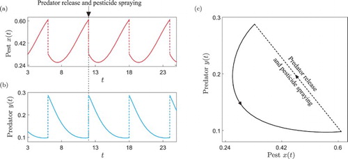9) In Figure 1 we present a periodic orbit of this system illustrating the solution segmentation introduced above. With this mathematical framework, we are now ready to carry out a detailed numerical investigation of this type of periodic response, via the continuation platform COCO.

Figure 1. Periodic solution of the impulsive system (9(9) $\begin{array}{rl}{u}^{\prime }\left(t\right)& =f_1\left(u\right(t),\alpha ),s\ne lT,s\ne T,\\ u\left(t^{+}\right)& =g_{\mathrm{P}-\mathrm{Spr}}\left(u\right(t^{-}),\alpha ),s=lT\left(\mathrm{pesticide}\mathrm{spraying}\right),\\ u\left(t^{+}\right)& =g_{\mathrm{Pr}-\mathrm{Re}}\left(u\right(t^{-}),\alpha ),s=T\left(\mathrm{natural}\mathrm{enemy}\mathrm{release}\right).\end{array}$(9) ) computed for the parameter values given in Table 1. Panels (a) and (b) show the time series of the pest (prey, red colour) and natural enemy (predator, blue colour) populations, respectively. The upper arrows indicate the pest control actions considered in the system. Panel (c) presents the phase plot of the periodic trajectory, showing the solution segments $I_1$ (pesticide spraying) and $I_2$ (predator release) defined in Section 3.3. In this case, the displayed periodic orbit has a cyclic solution signature $\{I_1,I_2\}$.

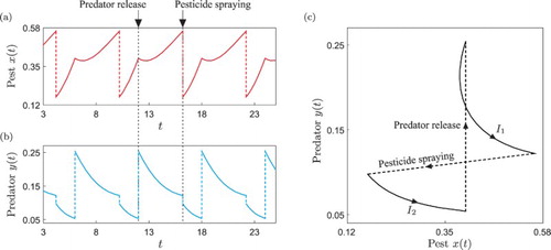
Table 1. Parameter values used for the numerical investigation.

Parameter	Symbol	Value
Pest's growth rate	r	1
Intrinsic predator's capturing rate	β	5.25
Weighting factor for saturation of predator's capturing rate	$k_x$	1.5
Weighting factor for interference among predators	$k_y$	1.125
Pest-to-predator conversion coefficient	C	0.5
Predator's mortality rate	μ	0.8
Impulse period	T	6
Tuning coefficient for pesticide spraying time	l	0.7
Amount of predators introduced per impulse period	d	0.2
Proportion of pest population killed by pesticides	${\sigma }_x$	0.7
Proportion of predator population killed by pesticides	${\sigma }_y$	0.2

3.4. Numerical analysis of the impulsive model via path-following methods

This section will present a detailed numerical study of the impulsive pest control scheme modelled by system (9(9) $\begin{array}{rl}{u}^{\prime }\left(t\right)& =f_1\left(u\right(t),\alpha ),s\ne lT,s\ne T,\\ u\left(t^{+}\right)& =g_{\mathrm{P}-\mathrm{Spr}}\left(u\right(t^{-}),\alpha ),s=lT\left(\mathrm{pesticide}\mathrm{spraying}\right),\\ u\left(t^{+}\right)& =g_{\mathrm{Pr}-\mathrm{Re}}\left(u\right(t^{-}),\alpha ),s=T\left(\mathrm{natural}\mathrm{enemy}\mathrm{release}\right).\end{array}$(9) ). Special attention will be given to the effect of the system parameters on $M_P$ (see Equation (7(7) $M_P:=\underset{0\le t\le T}{max}x\left(t\right),M_E:=\underset{0\le t\le T}{max}y\left(t\right),$(7) )), which can be used to monitor the amount of pest population in the ecosystem. The parameter values used in the numerical investigation are given in Table 1, which are taken from the previous publication by Zhang et al. [31], after the parameter transformation given in Equation (2(2) $\begin{array}{rl}\tilde{x}& =\frac{x}{K},\tilde{y}=\frac{y}{K},\tilde{\beta }=\frac{\beta K}{a},\\ {\tilde{k}}_x& =\frac{k_{x}K}{a},{\tilde{k}}_y=\frac{k_{y}K}{a},\tilde{d}=\frac{d}{K}.\end{array}$(2) ).

As already mentioned in Section 3.1, Zhang et al. [31] studied the stability of pest-free (also referred to as pest-eradication) periodic solutions of system (9(9) $\begin{array}{rl}{u}^{\prime }\left(t\right)& =f_1\left(u\right(t),\alpha ),s\ne lT,s\ne T,\\ u\left(t^{+}\right)& =g_{\mathrm{P}-\mathrm{Spr}}\left(u\right(t^{-}),\alpha ),s=lT\left(\mathrm{pesticide}\mathrm{spraying}\right),\\ u\left(t^{+}\right)& =g_{\mathrm{Pr}-\mathrm{Re}}\left(u\right(t^{-}),\alpha ),s=T\left(\mathrm{natural}\mathrm{enemy}\mathrm{release}\right).\end{array}$(9) ), as the impulse period T is varied. They determined a threshold $T_0$, depending on some of the remaining system parameters, so that for $T<T_0$ the pest-free solution is asymptotically stable, while for $T>T_0$ the system response is dominated by periodic solutions for which the pest and its natural enemies coexist. Specifically, Zhang et al. showed that the pest-free solution undergoes a change of stability (bifurcation) at $T=T_0$. However, they did not determine the actual type of bifurcation that produces this qualitative change, and this will be studied in more detail below via path-following (continuation) techniques.

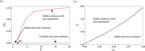
Let us then begin our study with the numerical continuation of the periodic solution shown in Figure 1 with respect to the impulse period T, as shown in Figure 2(a). As predicted by the analysis of Zhang et al., for low values of T the system presents stable pest-free solutions, as displayed in panel (d). If the impulse period is increased, a critical value $T_0\approx 2.2736$ is found, where the pest-free response loses stability. As was confirmed numerically, this bifurcation corresponds to a branching point [15] (labelled BP in the figure), and is the mechanism upon which an outbreak of the pest population can occur in the ecosystem. From the BP point, two branches of periodic solutions emanate, depicted as dashed and solid lines in the figure. The dashed curve represents unstable pest-free trajectories (as shown in Figure 2(e)), while the solid one corresponds to stable periodic solutions with pests and predators coexisting in the ecosystem, i.e. when an outbreak of the pest has occurred.

Figure 2. (a) One-parameter continuation of the periodic solution shown in Figure 1 of system (9(9) $\begin{array}{rl}{u}^{\prime }\left(t\right)& =f_1\left(u\right(t),\alpha ),s\ne lT,s\ne T,\\ u\left(t^{+}\right)& =g_{\mathrm{P}-\mathrm{Spr}}\left(u\right(t^{-}),\alpha ),s=lT\left(\mathrm{pesticide}\mathrm{spraying}\right),\\ u\left(t^{+}\right)& =g_{\mathrm{Pr}-\mathrm{Re}}\left(u\right(t^{-}),\alpha ),s=T\left(\mathrm{natural}\mathrm{enemy}\mathrm{release}\right).\end{array}$(9) ), with respect to the impulse period T. The solid and dashed lines stand for stable and unstable solutions, respectively, while the point labelled BP denotes a branching point. Panels (b)–(e) present time series for different values of the impulse period. Here, the pest and natural enemy populations are displayed with red and blue colours, respectively.

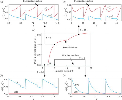
The solid branch shown in Figure 2(a) has a critical point $T_c\approx 10.4465$, where the curve loses smoothness. This singularity is produced by a change in the position of the peak value of the pest population. For $T<T_c$, the maximum amount of pest is attained exactly at the end of the segment $I_1$ (as in Figure 2(b)), while for $T>T_c$ the maximum value occurs at the end of the segment $I_2$ (see Figure 2(c)). Another feature of this curve is that the amount of pest population, measured by $M_P$, increases as T grows. From a practical point of view, this means that in order to keep low levels of pest population in the ecosystem, the impulse period should be chosen as small as possible, ideally below $T_0$. Nevertheless, having small impulse periods may imply high operation costs, since the control actions are carried out more frequently if T is reduced. In addition, smaller values of T also means an increasing use of pesticides in the ecosystem, and therefore a compromise should be made.

The next step in our numerical investigation is to study the model response when further system parameters are varied, see Figure 3. Panel (a) shows the numerical continuation of the periodic solution given in Figure 1 with respect to the intrinsic predator's capturing rate β. In this diagram, it can be observed that the peak predator population ($M_E$) is not significantly affected by this parameter and remains almost constant during the continuation. This is because a fixed amount of predators is periodically introduced into the ecosystem, and this impulsive perturbation has a stronger influence on the peak value of predators (see, e.g. Figure 2, panels (b)–(e)). On the other hand, the pest population shows a clear decreasing tendency when β is increased, which is consistent with the biological meaning of this parameter. A larger β means that the natural enemy enhances its ability to capture pest individuals, and that is the reason why the peak pest population ($M_P$) decreases significantly when β grows. Although this observation indicates that the parameter β can be effectively used to reduce the pest population, this may be in practice difficult or too expensive to implement, as it would require a certain mechanism to modify biological attributes of the natural enemy (via e.g. genetic engineering or selective breeding).

Figure 3. One-parameter continuation of the periodic solution shown in Figure 1 of system (9(9) $\begin{array}{rl}{u}^{\prime }\left(t\right)& =f_1\left(u\right(t),\alpha ),s\ne lT,s\ne T,\\ u\left(t^{+}\right)& =g_{\mathrm{P}-\mathrm{Spr}}\left(u\right(t^{-}),\alpha ),s=lT\left(\mathrm{pesticide}\mathrm{spraying}\right),\\ u\left(t^{+}\right)& =g_{\mathrm{Pr}-\mathrm{Re}}\left(u\right(t^{-}),\alpha ),s=T\left(\mathrm{natural}\mathrm{enemy}\mathrm{release}\right).\end{array}$(9) ), with respect to (a) β, (b) d and (c) l, showing the behaviour of the peak pest ($M_P$, red colour) and natural enemy ($M_E$, blue colour) populations, as defined in (7(7) $M_P:=\underset{0\le t\le T}{max}x\left(t\right),M_E:=\underset{0\le t\le T}{max}y\left(t\right),$(7) ). Panels (d) and (e) show time series of the pest population for l=0.3 and $l\approx 0.5464$ (where $M_P$ attains a minimum), respectively.

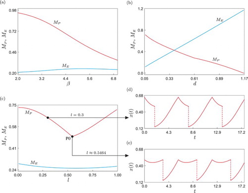
From a practical point of view, variations in the control parameters d and l may be more accessible for the users. As explained before, they represent the amount of predators periodically introduced into the ecosystem and the instant at which pesticides are applied, respectively. The behaviour of the peak pest and predator populations as d varies is shown in Figure 3(b). The result is biologically consistent in that the larger d, the higher the amount of predators in the ecosystem and the smaller the size of the pest population. This provides us with another effective way to control the pest, however, an increment in d may imply higher operation costs or negative consequences for other species present in the ecosystem, and therefore this parameter must also be chosen with certain precaution. On the other hand, the parameter l is the one that can be varied without causing significant ecological damage, as it controls just the instant at which pesticide is sprayed in each impulsive period. The effect of this parameter on the pest and predator populations is shown in Figure 3(c). The picture reveals an optimal point $l\approx 0.5464$ (labelled P0) where the peak size of pest population in the ecosystem achieves a minimum value $M_P\approx 0.5021$. The behaviour of the pest population at this optimal point is depicted in Figure 3(e), while panel (d) shows the system response at the test point l=0.3, for which the peak pest population is larger, although the impulsive period and the amount of introduced predators are exactly the same. These observations indicate that the performance of the pest control method can be improved by just changing the time at which pesticide is sprayed, without significantly increasing the ecological damage.

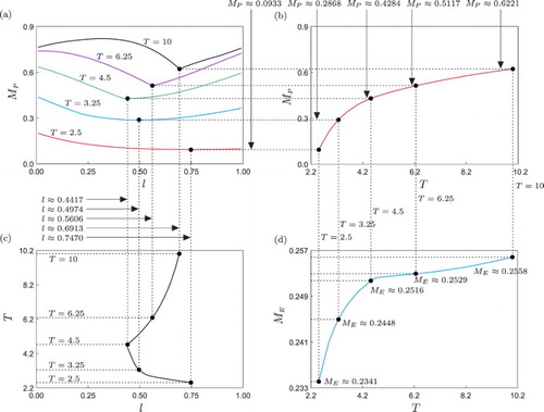
Let us now take a closer look into the optimal point obtained by varying the tuning coefficient for pesticide spraying l. Specifically, we will now investigate how the optimal value of l varies when a second parameter is changed, for instance, the impulse period T, which is a parameter that is usually modified in practical applications. The result of this analysis is presented in Figure 4, which depicts a series of curves computed via the continuation platform COCO. Panel (a) shows a family of curves obtained by recomputing the red curve displayed in Figure 3(c) for different values of T (between 2.5 and 10). These curves show how the peak pest population ($M_P$) behaves with respect to l, for the considered T's. As can be seen in this panel, the optimal value of l will indeed vary when T is changed, and the precise relationship between these parameters is computed in Figure 4(c), showing a nonlinear behaviour. During the computation of the optimal values of l as T varies, the resulting peak pest ($M_P$) and natural enemy ($M_E$) populations are monitored. As observed in panel (b), the minimal value of $M_P$ shows an increasing behaviour with respect to T, owing to the fact that a larger T means less frequent applications of the control measures. A similar relationship is observed for the peak natural enemy population $M_E$, which can be explained in terms of the larger time available to feed on the pest, when T increases, and the less frequent negative effect of the pesticide. The variation of $M_E$ with respect to T, however, is rather marginal (between 0.2341 and 0.2558), because the amount of natural enemies is mainly determined by the periodic introduction of these individuals, given by the parameter d=0.2.

Figure 4. Variation of the optimal point P0 shown in Figure 3(c), with respect to the impulse period T. Panel (a) shows a series of curves monitoring the peak pest population $M_P$ as a function of the tuning coefficient for pesticide spraying l, for different fixed values of T. Panel (b) depicts a curve representing the minimal values of $M_P$, obtained when T is varied. Analogously, panel (d) shows the corresponding levels of peak natural enemy population $M_E$. Panel (c) presents a curve showing the optimal values of l as the impulse period T is changed.

3.5. Further dynamical analysis of the pest control scheme

To conclude our numerical study of the impulsive model (9(9) $\begin{array}{rl}{u}^{\prime }\left(t\right)& =f_1\left(u\right(t),\alpha ),s\ne lT,s\ne T,\\ u\left(t^{+}\right)& =g_{\mathrm{P}-\mathrm{Spr}}\left(u\right(t^{-}),\alpha ),s=lT\left(\mathrm{pesticide}\mathrm{spraying}\right),\\ u\left(t^{+}\right)& =g_{\mathrm{Pr}-\mathrm{Re}}\left(u\right(t^{-}),\alpha ),s=T\left(\mathrm{natural}\mathrm{enemy}\mathrm{release}\right).\end{array}$(9) ), we will now employ both path-following methods and direct numerical integration in order to gain a deeper understanding of the dynamics of the impulsive pest control scheme considered in this section. The theoretical foundations for a numerical study of the impulsive system (9(9) $\begin{array}{rl}{u}^{\prime }\left(t\right)& =f_1\left(u\right(t),\alpha ),s\ne lT,s\ne T,\\ u\left(t^{+}\right)& =g_{\mathrm{P}-\mathrm{Spr}}\left(u\right(t^{-}),\alpha ),s=lT\left(\mathrm{pesticide}\mathrm{spraying}\right),\\ u\left(t^{+}\right)& =g_{\mathrm{Pr}-\mathrm{Re}}\left(u\right(t^{-}),\alpha ),s=T\left(\mathrm{natural}\mathrm{enemy}\mathrm{release}\right).\end{array}$(9) ) have been established by Zhang et al. [31]. They addressed the question of existence and uniqueness of nontrivial periodic solutions in terms of a fixed-point problem of a suitably defined operator. Following this approach, they also determined a threshold for the impulse period after which pest-free solutions lose stability (see previous section). Furthermore, in the conclusion part of Zhang et al. [31], the authors raised the question whether chaotic behaviour may be present in the system, and this will be precisely one of the main motivations for the numerical study presented in this section.

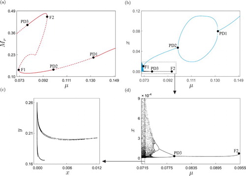
We begin our numerical study with the continuation of the periodic solution shown in Figure 1 with respect to the predator's mortality rate μ, see Figure 5(a). As the parameter is varied from larger to lower values, a first qualitative change is observed at $\mu \approx 0.1323$ (PD1). Here, one real Floquet multiplier of the periodic orbit crosses the complex unit circle from inside passing through $-1$. This phenomenon is referred to as a period-doubling (flip) bifurcation of limit cycles [15], and is characterized, in the supercritical case, by the birth of a stable periodic solution with twice the period of the original limit cycle, which in turn loses stability (schematically represented by the dashed line in Figure 5(a)). This unstable solution regains stability via another flip bifurcation at $\mu \approx 0.1001$ (PD2), where the critical Floquet multiplier comes back inside the unit circle and the stable periodic solution with double period disappears. If μ is further decreased, a turning point (also known as fold bifurcation) is found at $\mu \approx 0.0722$ (F1), in which case a pair of stable and unstable periodic orbits collide and then disappear for lower parameter values. From this point a branch (dashed segment) of unstable solutions is born, which finishes at F2 ($\mu \approx 0.0951$), where the system undergoes another fold bifurcation of limit cycles, and the periodic solution becomes stable. The last stability change is found at $\mu \approx 0.0792$ (PD3), corresponding to a supercritical flip bifurcation, from which a branch of unstable periodic solutions emerges. Another feature of the bifurcation diagram shown in Figure 5(a) is the presence of a parameter window $0.0792<\mu <0.0951$ for which the impulsive system possesses two stable periodic solutions that coexist (coexisting attractors [1]). This is produced by the interplay between the fold bifurcations F1 and F2, typically giving rise to hysteretic effects, as will be discussed below.

Figure 5. (a) Numerical continuation of the periodic solution shown in Figure 1 with respect to the predator's mortality rate μ. The points labelled PDi and Fi denote period-doubling and fold bifurcations of periodic orbits, respectively. Dashed and solid lines represent unstable and stable solutions of the system, respectively. (b) Bifurcation diagram computed via direct numerical integration of system (9(9) $\begin{array}{rl}{u}^{\prime }\left(t\right)& =f_1\left(u\right(t),\alpha ),s\ne lT,s\ne T,\\ u\left(t^{+}\right)& =g_{\mathrm{P}-\mathrm{Spr}}\left(u\right(t^{-}),\alpha ),s=lT\left(\mathrm{pesticide}\mathrm{spraying}\right),\\ u\left(t^{+}\right)& =g_{\mathrm{Pr}-\mathrm{Re}}\left(u\right(t^{-}),\alpha ),s=T\left(\mathrm{natural}\mathrm{enemy}\mathrm{release}\right).\end{array}$(9) ), for the parameter values given in Table 1. The black and blue colours mark the parameter sweeps in the increasing and decreasing directions, respectively. (c) Poincaré map associated with a chaotic attractor computed for $\mu =0.07206$. (d) Blow-up of the boxed region shown in panel (b).

In order to gain further insight into the dynamical behaviour of the pest control model, we will carry out a parametric study of the impulsive system (9(9) $\begin{array}{rl}{u}^{\prime }\left(t\right)& =f_1\left(u\right(t),\alpha ),s\ne lT,s\ne T,\\ u\left(t^{+}\right)& =g_{\mathrm{P}-\mathrm{Spr}}\left(u\right(t^{-}),\alpha ),s=lT\left(\mathrm{pesticide}\mathrm{spraying}\right),\\ u\left(t^{+}\right)& =g_{\mathrm{Pr}-\mathrm{Re}}\left(u\right(t^{-}),\alpha ),s=T\left(\mathrm{natural}\mathrm{enemy}\mathrm{release}\right).\end{array}$(9) ) via direct numerical integration, when the predator's mortality rate μ is varied. For this purpose, we fix a starting value for μ and then integrate the system over 300 impulse periods to allow for the decay of transients. After this, we extend the numerical integration for another interval of 100 periods and store samples of the extended solution at the times $t=(i+ϵ-1)T$, $i=1,2,\dots ,100$, with $0<ϵ<l$ being a fixed shift coefficient. This parameter is introduced so as to avoid sampling the solution at the impulse times $t=(n+l-1)T$ and t=nT, $n\in \mathbb{N}$. Next, μ is increased (or decreased, depending on the sweep direction) by a small amount and then the same procedure is repeated, now using the last sample of the previous step as initial value. This process terminates when a predefined final value for μ is reached.

The result of the numerical procedure described above is shown in Figure 5(b). The picture confirms the qualitative changes (bifurcations) predicted in panel (a), labelled PDi and Fi. In particular, the bifurcation diagram shown in panel (b) allows us to visualize the creation and disappearance of orbits with double period, observed at the flip bifurcations $\mu \approx 0.1001$ and $\mu \approx 0.1323$ detected before. The increasing (black) and decreasing (blue) parameter sweeps reveal the presence of parameter hysteresis in the system, produced by the coexistence of periodic attractors, as predicted above. The blow-up of the boxed part of the bifurcation diagram, shown in panel (d), contains the bifurcation points PD3 and F2 found in Figure 5(a). These two points define a parameter window in which a stable orbit of period T survives. When μ decreases through PD3, the period-T solution becomes unstable and a stable periodic orbit of twice the period appears. If μ is further reduced, the period-$2T$ trajectory loses stability via another flip bifurcation ($\mu \approx 0.0755$), giving rise to a stable periodic solution of period $4T$. This phenomenon repeats again and again as the parameter continues to decrease, until a critical value is reached where the flip bifurcations accumulate, leading to chaotic behaviour. This infinite sequence of period-doubling bifurcations caused by the variation of a parameter over a finite interval is referred to as a period-doubling cascade, and is one of the classical routes to chaos in Dynamical Systems [1]. Figure 5(c) depicts the intersection of a chaotic attractor of the impulsive system (9(9) $\begin{array}{rl}{u}^{\prime }\left(t\right)& =f_1\left(u\right(t),\alpha ),s\ne lT,s\ne T,\\ u\left(t^{+}\right)& =g_{\mathrm{P}-\mathrm{Spr}}\left(u\right(t^{-}),\alpha ),s=lT\left(\mathrm{pesticide}\mathrm{spraying}\right),\\ u\left(t^{+}\right)& =g_{\mathrm{Pr}-\mathrm{Re}}\left(u\right(t^{-}),\alpha ),s=T\left(\mathrm{natural}\mathrm{enemy}\mathrm{release}\right).\end{array}$(9) ) with a Poincaré section for $\mu =0.07206$, showing a well-known fingered structure [9, 32]. This numerical study gives a positive answer to one of the open questions outlined by Zhang et al. [31] related to the existence of chaotic behaviour in the system, since we have identified a parameter set and a mechanism upon which chaos can appear in the pest control model.

4. A numerical comparison with an impulsive pest control model with state-dependent pesticide mortality

The previous section was devoted to the application of specialized numerical techniques in order to study the dynamical behaviour of model (3(3) $\left\{\begin{array}{l}\left.\begin{array}{rl}{x}^{\prime }\left(t\right)& =rx\left(t\right)\left(1-x\left(t\right)\right)-\frac{\beta x\left(t\right)y\left(t\right)}{1+k_{x}x\left(t\right)+k_{y}y\left(t\right)},\\ y^{\prime }\left(t\right)& =\frac{C\beta x\left(t\right)y\left(t\right)}{1+k_{x}x\left(t\right)+k_{y}y\left(t\right)}-\mu y\left(t\right),\end{array}\right\}t\ne (n+l-1)T,t\ne nT,\\ \left.\begin{array}{rl}x\left(t^{+}\right)& =(1-{\sigma }_x)x\left(t^{-}\right),\\ y\left(t^{+}\right)& =(1-{\sigma }_y)y\left(t^{-}\right),\end{array}\right\}t=(n+l-1)T\left(\mathrm{pesticide}\mathrm{spraying}\right),\\ \left.\begin{array}{rl}x\left(t^{+}\right)& =x\left(t^{-}\right),\\ y\left(t^{+}\right)& =y\left(t^{-}\right)+d,\end{array}\right\}t=nT,n\in \mathbb{N}\left(\mathrm{natural}\mathrm{enemy}\mathrm{release}\right),\end{array}\right.$(3) ), which describes a pest control scheme in the framework of IPM. The numerical investigation was mainly focused on determining the influence of selected model parameters on the pest and natural enemy populations. Here, the main motivation was to identify general strategies so as to reduce the presence of the pest, while taking into account possible negative ecological effects. Now our next goal will be to investigate the extent to which such strategies remain valid when the assumed ecosystem changes. For this purpose, we will carry out a comparative numerical study based on an impulsive pest control model that shares some common features with the scenario considered in the previous section. The main difference, however, will lie on how the pest control actions are executed and the way the employed pesticides affect the populations, as will be described in detail below.

4.1. Model description

As in the previous case, the model to be analysed in this section considers a combination of two pest control techniques. The first one is the periodic introduction of natural enemies into the ecosystem, which falls into the category of biological control and is assumed to be ecologically benign. On the contrary, the second control method is based on the application of pesticides, which is regarded as environmentally harmful. The ecological scenario, proposed by Qin et al. [21], is mathematically described as follows: (10) $\left\{\begin{array}{ll}\left.\begin{array}{rl}{x}^{\prime }\left(t\right)& =rx\left(t\right)\left(1-\frac{x\left(t\right)}{K}\right)-\frac{\beta x\left(t\right)y\left(t\right)}{a+x\left(t\right)},\\ y^{\prime }\left(t\right)& =\frac{C\beta x\left(t\right)y\left(t\right)}{a+x\left(t\right)}-\mu y\left(t\right),\end{array}\right\}& t\ne nT,\\ \left.\begin{array}{rl}x\left(t^{+}\right)& =\left(1-p_x\left(x\left(t^{-}\right)\right)\right)x\left(t^{-}\right),\\ y\left(t^{+}\right)& =\left(1-p_y\left(y\left(t^{-}\right)\right)\right)y\left(t^{-}\right)+d,\end{array}\right\}& t=nT(\mathrm{pesticide}\mathrm{spraying}\mathrm{and}\\ & \mathrm{natural}\mathrm{enemy}\mathrm{release}),\end{array}\right.$(10) where (11) $p_x\left(u\right):=\frac{{\sigma }_x}{1+\gamma {\mathrm{e}}^{-\lambda u}},p_y\left(u\right):=\frac{{\sigma }_y}{1+\gamma {\mathrm{e}}^{-\lambda u}},$(11) with $u\ge 0$, $0\le {\sigma }_{x,y}\le 1$, $\lambda >0$, $\gamma >0$, $n\in \mathbb{N}$. As before, x and y represent the pest (prey) and natural enemy (predator) population, respectively, and the parameters have a similar meaning as in model (1(1) $\left\{\begin{array}{l}\left.\begin{array}{rl}{x}^{\prime }\left(t\right)& =rx\left(t\right)\left(1-\frac{x\left(t\right)}{K}\right)-\frac{\beta x\left(t\right)y\left(t\right)}{a+k_{x}x\left(t\right)+k_{y}y\left(t\right)},\\ y^{\prime }\left(t\right)& =\frac{C\beta x\left(t\right)y\left(t\right)}{a+k_{x}x\left(t\right)+k_{y}y\left(t\right)}-\mu y\left(t\right),\end{array}\right\}t\ne (n+l-1)T,t\ne nT,\\ \left.\begin{array}{rl}x\left(t^{+}\right)& =(1-{\sigma }_x)x\left(t^{-}\right),\\ y\left(t^{+}\right)& =(1-{\sigma }_y)y\left(t^{-}\right),\end{array}\right\}t=(n+l-1)T\left(\mathrm{pesticide}\mathrm{spraying}\right),\\ \left.\begin{array}{rl}x\left(t^{+}\right)& =x\left(t^{-}\right),\\ y\left(t^{+}\right)& =y\left(t^{-}\right)+d,\end{array}\right\}t=nT,n\in \mathbb{N}\left(\mathrm{natural}\mathrm{enemy}\mathrm{release}\right),\end{array}\right.$(1) ). In the present case, the predator population feeds on the pest according to a Holling type-II trophic function [11], where β is the maximum predator's capturing rate and a stands for the pest population density at which the capturing rate is half the saturation value. The main difference with the ecological scenario considered in the previous section is that now the control actions, pesticide spraying and predator release, are carried out simultaneously, at every t=nT. In addition, the proportion of pest and predator population killed by the pesticide is now assumed to be state dependent, given by the functions $p_{x,y}$ defined in Equation (11(11) $p_x\left(u\right):=\frac{{\sigma }_x}{1+\gamma {\mathrm{e}}^{-\lambda u}},p_y\left(u\right):=\frac{{\sigma }_y}{1+\gamma {\mathrm{e}}^{-\lambda u}},$(11) ), which can be interpreted as follows. The parameters ${\sigma }_{x,y}$ represent a maximum pesticide mortality that is achieved for large population sizes (i.e. $u\to \mathrm{\infty }$), in which case the population is assumed to be more vulnerable to the pesticide. On the contrary, when only few individuals are present (i.e. $u\approx 0$), the pesticide mortality is low (reduced by the factor $1/(1+\gamma )$), because, for instance, the low number of individuals is not properly reached by the pesticide or they can hide during the spraying. The effectiveness of this protection ability is measured by the parameter γ, while λ determines the population size from which this ability becomes meaningful.

4.2. Basic mathematical set-up

The numerical study of the impulsive system (10(10) $\left\{\begin{array}{ll}\left.\begin{array}{rl}{x}^{\prime }\left(t\right)& =rx\left(t\right)\left(1-\frac{x\left(t\right)}{K}\right)-\frac{\beta x\left(t\right)y\left(t\right)}{a+x\left(t\right)},\\ y^{\prime }\left(t\right)& =\frac{C\beta x\left(t\right)y\left(t\right)}{a+x\left(t\right)}-\mu y\left(t\right),\end{array}\right\}& t\ne nT,\\ \left.\begin{array}{rl}x\left(t^{+}\right)& =\left(1-p_x\left(x\left(t^{-}\right)\right)\right)x\left(t^{-}\right),\\ y\left(t^{+}\right)& =\left(1-p_y\left(y\left(t^{-}\right)\right)\right)y\left(t^{-}\right)+d,\end{array}\right\}& t=nT(\mathrm{pesticide}\mathrm{spraying}\mathrm{and}\\ & \mathrm{natural}\mathrm{enemy}\mathrm{release}),\end{array}\right.$(10) ) will be carried out following the approach employed in Section 3. As before, it is convenient to introduce a scaling of the variables and parameters according to the formulae (12) $\begin{array}{rl}\tilde{x}& =\frac{x}{K},\tilde{y}=\frac{y}{K},\tilde{\beta }=\frac{\beta K}{a},\\ {\tilde{k}}_x& =\frac{K}{a},\tilde{\lambda }=\lambda K,\tilde{d}=\frac{d}{K}.\end{array}$(12) After applying these transformations, the continuous dynamics of the impulsive model (10(10) $\left\{\begin{array}{ll}\left.\begin{array}{rl}{x}^{\prime }\left(t\right)& =rx\left(t\right)\left(1-\frac{x\left(t\right)}{K}\right)-\frac{\beta x\left(t\right)y\left(t\right)}{a+x\left(t\right)},\\ y^{\prime }\left(t\right)& =\frac{C\beta x\left(t\right)y\left(t\right)}{a+x\left(t\right)}-\mu y\left(t\right),\end{array}\right\}& t\ne nT,\\ \left.\begin{array}{rl}x\left(t^{+}\right)& =\left(1-p_x\left(x\left(t^{-}\right)\right)\right)x\left(t^{-}\right),\\ y\left(t^{+}\right)& =\left(1-p_y\left(y\left(t^{-}\right)\right)\right)y\left(t^{-}\right)+d,\end{array}\right\}& t=nT(\mathrm{pesticide}\mathrm{spraying}\mathrm{and}\\ & \mathrm{natural}\mathrm{enemy}\mathrm{release}),\end{array}\right.$(10) ) can be characterized by the equation (cf. Equation (4(4) $u^{\prime }\left(t\right)=f_1\left(u\right(t),\alpha ):=\left(\begin{array}{c}rx\left(t\right)\left(1-x\left(t\right)\right)-\frac{\beta x\left(t\right)y\left(t\right)}{1+k_{x}x\left(t\right)+k_{y}y\left(t\right)}\\ \frac{C\beta x\left(t\right)y\left(t\right)}{1+k_{x}x\left(t\right)+k_{y}y\left(t\right)}-\mu y\left(t\right)\\ 1\end{array}\right).$(4) )) (13) $u^{\prime }\left(t\right)=f_2\left(u\right(t),\omega ):=\left(\begin{array}{c}rx\left(t\right)\left(1-x\left(t\right)\right)-\frac{\beta x\left(t\right)y\left(t\right)}{1+k_{x}x\left(t\right)}\\ \frac{C\beta x\left(t\right)y\left(t\right)}{1+k_{x}x\left(t\right)}-\mu y\left(t\right)\\ 1\end{array}\right),$(13) where the tildes have been dropped and $\omega :=(r,\beta ,k_x,C,\mu ,\gamma ,\lambda ,d,T,{\sigma }_x,{\sigma }_y)\in ({\mathbb{R}}^{+}{)}^9\times [0,1]\times [0,1]$ denotes the vector of parameters, while u is the same state variable defined previously. The impulsive control actions of pesticide spraying and natural enemy release can be represented by the jump function (cf. Equations (5(5) $g_{\mathrm{P}-\mathrm{Spr}}(u,\alpha ):=\left(\begin{array}{c}(1-{\sigma }_x)x\\ (1-{\sigma }_y)y\\ s\end{array}\right),$(5) ), (6(6) $g_{\mathrm{Pr}-\mathrm{Re}}(u,\alpha ):=\left(\begin{array}{c}x\\ y+d\\ s-T\end{array}\right).$(6) ) and (10(10) $\left\{\begin{array}{ll}\left.\begin{array}{rl}{x}^{\prime }\left(t\right)& =rx\left(t\right)\left(1-\frac{x\left(t\right)}{K}\right)-\frac{\beta x\left(t\right)y\left(t\right)}{a+x\left(t\right)},\\ y^{\prime }\left(t\right)& =\frac{C\beta x\left(t\right)y\left(t\right)}{a+x\left(t\right)}-\mu y\left(t\right),\end{array}\right\}& t\ne nT,\\ \left.\begin{array}{rl}x\left(t^{+}\right)& =\left(1-p_x\left(x\left(t^{-}\right)\right)\right)x\left(t^{-}\right),\\ y\left(t^{+}\right)& =\left(1-p_y\left(y\left(t^{-}\right)\right)\right)y\left(t^{-}\right)+d,\end{array}\right\}& t=nT(\mathrm{pesticide}\mathrm{spraying}\mathrm{and}\\ & \mathrm{natural}\mathrm{enemy}\mathrm{release}),\end{array}\right.$(10) )) (14) $g_{\mathrm{Cont}}(u,\omega ):=\left(\begin{array}{c}\left(1-p_x\left(x\right)\right)x\\ \left(1-p_y\left(y\right)\right)y+d\\ s-T\end{array}\right),$(14) In this setting, the impulsive pest control model can be expressed as a hybrid dynamical system as follows (cf. Equations (9(9) $\begin{array}{rl}{u}^{\prime }\left(t\right)& =f_1\left(u\right(t),\alpha ),s\ne lT,s\ne T,\\ u\left(t^{+}\right)& =g_{\mathrm{P}-\mathrm{Spr}}\left(u\right(t^{-}),\alpha ),s=lT\left(\mathrm{pesticide}\mathrm{spraying}\right),\\ u\left(t^{+}\right)& =g_{\mathrm{Pr}-\mathrm{Re}}\left(u\right(t^{-}),\alpha ),s=T\left(\mathrm{natural}\mathrm{enemy}\mathrm{release}\right).\end{array}$(9) ) and (10(10) $\left\{\begin{array}{ll}\left.\begin{array}{rl}{x}^{\prime }\left(t\right)& =rx\left(t\right)\left(1-\frac{x\left(t\right)}{K}\right)-\frac{\beta x\left(t\right)y\left(t\right)}{a+x\left(t\right)},\\ y^{\prime }\left(t\right)& =\frac{C\beta x\left(t\right)y\left(t\right)}{a+x\left(t\right)}-\mu y\left(t\right),\end{array}\right\}& t\ne nT,\\ \left.\begin{array}{rl}x\left(t^{+}\right)& =\left(1-p_x\left(x\left(t^{-}\right)\right)\right)x\left(t^{-}\right),\\ y\left(t^{+}\right)& =\left(1-p_y\left(y\left(t^{-}\right)\right)\right)y\left(t^{-}\right)+d,\end{array}\right\}& t=nT(\mathrm{pesticide}\mathrm{spraying}\mathrm{and}\\ & \mathrm{natural}\mathrm{enemy}\mathrm{release}),\end{array}\right.$(10) )) (15) $\begin{array}{rl}{u}^{\prime }\left(t\right)& =f_2\left(u\right(t),\omega ),s\ne T,\\ u\left(t^{+}\right)& =g_{\mathrm{Cont}}\left(u\right(t^{-}),\omega ),s=T\left(\mathrm{pesticide}\mathrm{spraying}\mathrm{and}\mathrm{natural}\mathrm{enemy}\mathrm{release}\right),\end{array}$(15) where s represents again an auxiliary variable used to monitor the impulse times and is kept within the interval $[0,T]$ during operation.

4.3. Numerical analysis of the impulsive model and comparison with the previous results

Our main concern in the present section will be to investigate the effect of parameter variations on the periodic response of the pest control model described by the impulsive system (15(15) $\begin{array}{rl}{u}^{\prime }\left(t\right)& =f_2\left(u\right(t),\omega ),s\ne T,\\ u\left(t^{+}\right)& =g_{\mathrm{Cont}}\left(u\right(t^{-}),\omega ),s=T\left(\mathrm{pesticide}\mathrm{spraying}\mathrm{and}\mathrm{natural}\mathrm{enemy}\mathrm{release}\right),\end{array}$(15) ). For this purpose, we will employ path-following algorithms specialized for hybrid dynamical systems, implemented via the continuation platform COCO, as described before. The starting point of our numerical study is the periodic response shown in Figure 6, obtained for the parameter set given in Table 1, so as to be able to compare the dynamical response of the impulsive control schemes described by the models (9(9) $\begin{array}{rl}{u}^{\prime }\left(t\right)& =f_1\left(u\right(t),\alpha ),s\ne lT,s\ne T,\\ u\left(t^{+}\right)& =g_{\mathrm{P}-\mathrm{Spr}}\left(u\right(t^{-}),\alpha ),s=lT\left(\mathrm{pesticide}\mathrm{spraying}\right),\\ u\left(t^{+}\right)& =g_{\mathrm{Pr}-\mathrm{Re}}\left(u\right(t^{-}),\alpha ),s=T\left(\mathrm{natural}\mathrm{enemy}\mathrm{release}\right).\end{array}$(9) ) and (15(15) $\begin{array}{rl}{u}^{\prime }\left(t\right)& =f_2\left(u\right(t),\omega ),s\ne T,\\ u\left(t^{+}\right)& =g_{\mathrm{Cont}}\left(u\right(t^{-}),\omega ),s=T\left(\mathrm{pesticide}\mathrm{spraying}\mathrm{and}\mathrm{natural}\mathrm{enemy}\mathrm{release}\right),\end{array}$(15) ). On the other hand, the parameters describing the protection ability from the pesticide are taken from the study by Qin et al. [21] ($\lambda =\gamma =1$).

Figure 6. Periodic solution of the impulsive system (15(15) $\begin{array}{rl}{u}^{\prime }\left(t\right)& =f_2\left(u\right(t),\omega ),s\ne T,\\ u\left(t^{+}\right)& =g_{\mathrm{Cont}}\left(u\right(t^{-}),\omega ),s=T\left(\mathrm{pesticide}\mathrm{spraying}\mathrm{and}\mathrm{natural}\mathrm{enemy}\mathrm{release}\right),\end{array}$(15) ) computed for the parameter values given in Table 1, and for $\gamma =\lambda =1$. Panels (a) and (b) show the time series of the pest (prey, red colour) and natural enemy (predator, blue colour) populations, respectively. The upper arrow indicates the pest control actions considered in the system. Panel (c) presents the phase plot of the periodic trajectory.

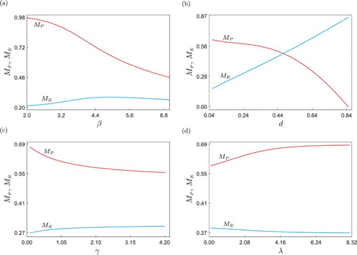
Let us investigate first the effect of the impulse period T on the system response. The result can be seen in Figure 7, showing the numerical continuation of the periodic orbit displayed in Figure 6. Similarly to case studied in Figure 2, the dynamics of the system is influenced by the presence of a branching point (BP). For low values of T, there exists a branch of stable periodic solutions for which the ecosystem remains pest-free. As the parameter increases, a critical value $T_0\approx 1.6980$ is found, where the pest-free solution loses stability due to the branching point. Again, this point defines the impulse period above which a pest outbreak can take place, as can be seen from the sharp increase of $M_P$ (peak pest population) right after the BP point. Therefore, the BP point can be interpreted as a limit point that divide the system response into two scenarios: a first one where the pest is effectively eradicated from the ecosystem by the control actions ($T<T_0$), and the second one, corresponding to the case when the pest and the natural enemy coexist ($T>T_0$). As before, we observe that $M_P$ shows an increasing behaviour when T grows, owing to the fact that a larger T means less frequent applications of the control measures.

Figure 7. (a) One-parameter continuation of the periodic solution shown in Figure 6 of system (15(15) $\begin{array}{rl}{u}^{\prime }\left(t\right)& =f_2\left(u\right(t),\omega ),s\ne T,\\ u\left(t^{+}\right)& =g_{\mathrm{Cont}}\left(u\right(t^{-}),\omega ),s=T\left(\mathrm{pesticide}\mathrm{spraying}\mathrm{and}\mathrm{natural}\mathrm{enemy}\mathrm{release}\right),\end{array}$(15) ), with respect to the impulse period T. The solid and dashed lines stand for stable and unstable solutions, respectively, while the point labelled BP denotes a branching point. (b) Two-parameter continuation of the BP point found in panel (a), with respect to T and ${\sigma }_x$.

Despite the similarities between the bifurcation scenarios shown in Figures 2 and 7, we observe a clear difference between the values at which the branching point occurs ($T_0\approx 2.2736$ and $T_0\approx 1.6980$, respectively). This means that for the current ecological scenario (model (15(15) $\begin{array}{rl}{u}^{\prime }\left(t\right)& =f_2\left(u\right(t),\omega ),s\ne T,\\ u\left(t^{+}\right)& =g_{\mathrm{Cont}}\left(u\right(t^{-}),\omega ),s=T\left(\mathrm{pesticide}\mathrm{spraying}\mathrm{and}\mathrm{natural}\mathrm{enemy}\mathrm{release}\right),\end{array}$(15) )), the pest control actions have to be applied more frequently than for case described by model (9(9) $\begin{array}{rl}{u}^{\prime }\left(t\right)& =f_1\left(u\right(t),\alpha ),s\ne lT,s\ne T,\\ u\left(t^{+}\right)& =g_{\mathrm{P}-\mathrm{Spr}}\left(u\right(t^{-}),\alpha ),s=lT\left(\mathrm{pesticide}\mathrm{spraying}\right),\\ u\left(t^{+}\right)& =g_{\mathrm{Pr}-\mathrm{Re}}\left(u\right(t^{-}),\alpha ),s=T\left(\mathrm{natural}\mathrm{enemy}\mathrm{release}\right).\end{array}$(9) ), in order to eradicate the pest completely. This difference can be explained in terms of how the pesticide affects the pest. In contrast to the previous model (9(9) $\begin{array}{rl}{u}^{\prime }\left(t\right)& =f_1\left(u\right(t),\alpha ),s\ne lT,s\ne T,\\ u\left(t^{+}\right)& =g_{\mathrm{P}-\mathrm{Spr}}\left(u\right(t^{-}),\alpha ),s=lT\left(\mathrm{pesticide}\mathrm{spraying}\right),\\ u\left(t^{+}\right)& =g_{\mathrm{Pr}-\mathrm{Re}}\left(u\right(t^{-}),\alpha ),s=T\left(\mathrm{natural}\mathrm{enemy}\mathrm{release}\right).\end{array}$(9) ), model (15(15) $\begin{array}{rl}{u}^{\prime }\left(t\right)& =f_2\left(u\right(t),\omega ),s\ne T,\\ u\left(t^{+}\right)& =g_{\mathrm{Cont}}\left(u\right(t^{-}),\omega ),s=T\left(\mathrm{pesticide}\mathrm{spraying}\mathrm{and}\mathrm{natural}\mathrm{enemy}\mathrm{release}\right),\end{array}$(15) ) assumes that the pesticide mortality depends on the amount of individuals at the moment of application. This means that, for the same value of the parameter ${\sigma }_x$, the effective pesticide mortality is smaller for the model (15(15) $\begin{array}{rl}{u}^{\prime }\left(t\right)& =f_2\left(u\right(t),\omega ),s\ne T,\\ u\left(t^{+}\right)& =g_{\mathrm{Cont}}\left(u\right(t^{-}),\omega ),s=T\left(\mathrm{pesticide}\mathrm{spraying}\mathrm{and}\mathrm{natural}\mathrm{enemy}\mathrm{release}\right),\end{array}$(15) ), as can be seen from Equation (11(11) $p_x\left(u\right):=\frac{{\sigma }_x}{1+\gamma {\mathrm{e}}^{-\lambda u}},p_y\left(u\right):=\frac{{\sigma }_y}{1+\gamma {\mathrm{e}}^{-\lambda u}},$(11) ). In order to investigate this matter further, we carried out a two-parameter continuation of the branching point BP detected in system (15(15) $\begin{array}{rl}{u}^{\prime }\left(t\right)& =f_2\left(u\right(t),\omega ),s\ne T,\\ u\left(t^{+}\right)& =g_{\mathrm{Cont}}\left(u\right(t^{-}),\omega ),s=T\left(\mathrm{pesticide}\mathrm{spraying}\mathrm{and}\mathrm{natural}\mathrm{enemy}\mathrm{release}\right),\end{array}$(15) ), with respect to T and ${\sigma }_x$. The result is shown in Figure 7(b). The picture displays a curve representing the combinations of T and ${\sigma }_x$ for which a branching point occurs. Hence, the curve divides locally the parameter space into two regions: one for which the pest is completely eradicated from the ecosystem (below the curve), and one where the pest and its natural enemy coexist (above the curve). According to the observed result, we can conclude that the larger the pesticide mortality (given by a larger ${\sigma }_x$), the higher the critical impulse period ($T_0$) after which a pest outbreak occurs. On the other hand, a weaker pesticide (i.e. with a smaller ${\sigma }_x$) will require more frequent applications in order to eradicate the pest, which is mathematically explained by the earlier occurrence of the branching point, as seen in Figure 7(b).

Next, we will investigate the response of model (15(15) $\begin{array}{rl}{u}^{\prime }\left(t\right)& =f_2\left(u\right(t),\omega ),s\ne T,\\ u\left(t^{+}\right)& =g_{\mathrm{Cont}}\left(u\right(t^{-}),\omega ),s=T\left(\mathrm{pesticide}\mathrm{spraying}\mathrm{and}\mathrm{natural}\mathrm{enemy}\mathrm{release}\right),\end{array}$(15) ) under further parameter variations, as shown in Figure 8. The picture presents the behaviour of the peak pest ($M_P$) and natural enemy ($M_E$) populations when β, d, γ and λ are varied, similarly to the numerical study presented in Figure 3. As before, the effect of the parameter β on the pest population is as expected, since a larger β means a higher ability of the predators to capture pest individuals, due to which $M_P$ shows a decreasing behaviour. Likewise, the behaviour of $M_P$ and $M_E$ follows closely the one observed for the previous model (9(9) $\begin{array}{rl}{u}^{\prime }\left(t\right)& =f_1\left(u\right(t),\alpha ),s\ne lT,s\ne T,\\ u\left(t^{+}\right)& =g_{\mathrm{P}-\mathrm{Spr}}\left(u\right(t^{-}),\alpha ),s=lT\left(\mathrm{pesticide}\mathrm{spraying}\right),\\ u\left(t^{+}\right)& =g_{\mathrm{Pr}-\mathrm{Re}}\left(u\right(t^{-}),\alpha ),s=T\left(\mathrm{natural}\mathrm{enemy}\mathrm{release}\right).\end{array}$(9) ), when the amount of natural enemies introduced in the system (d) is varied, see Figures 3(b) and 8(b). A noticeable difference, however, is observed at the value of d for which $M_P$ becomes zero, i.e. when the pest is eradicated. For model (9(9) $\begin{array}{rl}{u}^{\prime }\left(t\right)& =f_1\left(u\right(t),\alpha ),s\ne lT,s\ne T,\\ u\left(t^{+}\right)& =g_{\mathrm{P}-\mathrm{Spr}}\left(u\right(t^{-}),\alpha ),s=lT\left(\mathrm{pesticide}\mathrm{spraying}\right),\\ u\left(t^{+}\right)& =g_{\mathrm{Pr}-\mathrm{Re}}\left(u\right(t^{-}),\alpha ),s=T\left(\mathrm{natural}\mathrm{enemy}\mathrm{release}\right).\end{array}$(9) ) this occurs for $d\approx 1.1615$, whereas for the current system (15(15) $\begin{array}{rl}{u}^{\prime }\left(t\right)& =f_2\left(u\right(t),\omega ),s\ne T,\\ u\left(t^{+}\right)& =g_{\mathrm{Cont}}\left(u\right(t^{-}),\omega ),s=T\left(\mathrm{pesticide}\mathrm{spraying}\mathrm{and}\mathrm{natural}\mathrm{enemy}\mathrm{release}\right),\end{array}$(15) ), the critical value is smaller ($d\approx 0.8493$). These values indicate that in order to eradicate the pest from the ecosystem, a larger amount of predators is required for the control scheme considered in model (9(9) $\begin{array}{rl}{u}^{\prime }\left(t\right)& =f_1\left(u\right(t),\alpha ),s\ne lT,s\ne T,\\ u\left(t^{+}\right)& =g_{\mathrm{P}-\mathrm{Spr}}\left(u\right(t^{-}),\alpha ),s=lT\left(\mathrm{pesticide}\mathrm{spraying}\right),\\ u\left(t^{+}\right)& =g_{\mathrm{Pr}-\mathrm{Re}}\left(u\right(t^{-}),\alpha ),s=T\left(\mathrm{natural}\mathrm{enemy}\mathrm{release}\right).\end{array}$(9) ). This can be explained in terms of the trophic interaction between the pest and its natural enemy, which is described by the Beddington–DeAngelis functional in system (9(9) $\begin{array}{rl}{u}^{\prime }\left(t\right)& =f_1\left(u\right(t),\alpha ),s\ne lT,s\ne T,\\ u\left(t^{+}\right)& =g_{\mathrm{P}-\mathrm{Spr}}\left(u\right(t^{-}),\alpha ),s=lT\left(\mathrm{pesticide}\mathrm{spraying}\right),\\ u\left(t^{+}\right)& =g_{\mathrm{Pr}-\mathrm{Re}}\left(u\right(t^{-}),\alpha ),s=T\left(\mathrm{natural}\mathrm{enemy}\mathrm{release}\right).\end{array}$(9) ). As explained before, this functional considers competition among the natural enemies, a feature that is rather absent in the ecosystem considered in model (15(15) $\begin{array}{rl}{u}^{\prime }\left(t\right)& =f_2\left(u\right(t),\omega ),s\ne T,\\ u\left(t^{+}\right)& =g_{\mathrm{Cont}}\left(u\right(t^{-}),\omega ),s=T\left(\mathrm{pesticide}\mathrm{spraying}\mathrm{and}\mathrm{natural}\mathrm{enemy}\mathrm{release}\right),\end{array}$(15) ), where the predator–prey interaction is determined by a Holling type-II trophic function, which makes the natural enemies more effective in controlling the pest.

Figure 8. One-parameter continuation of the periodic solution shown in Figure 6 of system (15(15) $\begin{array}{rl}{u}^{\prime }\left(t\right)& =f_2\left(u\right(t),\omega ),s\ne T,\\ u\left(t^{+}\right)& =g_{\mathrm{Cont}}\left(u\right(t^{-}),\omega ),s=T\left(\mathrm{pesticide}\mathrm{spraying}\mathrm{and}\mathrm{natural}\mathrm{enemy}\mathrm{release}\right),\end{array}$(15) ), with respect to (a) β, (b) d, (c) γ and (d) λ, showing the behaviour of the peak pest ($M_P$, red colour) and natural enemy ($M_E$, blue colour) populations.

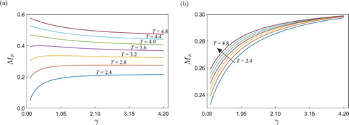
We will now discuss the influence of the parameters γ and λ on the system behaviour, which describe the ability of both pest and natural enemy populations to protect themselves from the pesticides. Let us first consider the effect of the parameters on the natural enemy population only, given by the blue curves shown in Figure 8(c, d). In panel (c) we observe a growing behaviour of the natural enemy population when γ increases, although this effect is only marginally noticeable due to the periodic introduction of natural enemies into the ecosystem. Furthermore, a decreasing behaviour of the natural enemy population is observed in Figure 8(d), for increasing λ. Both results are perfectly consistent with the pesticide mortality assumed for model (15(15) $\begin{array}{rl}{u}^{\prime }\left(t\right)& =f_2\left(u\right(t),\omega ),s\ne T,\\ u\left(t^{+}\right)& =g_{\mathrm{Cont}}\left(u\right(t^{-}),\omega ),s=T\left(\mathrm{pesticide}\mathrm{spraying}\mathrm{and}\mathrm{natural}\mathrm{enemy}\mathrm{release}\right),\end{array}$(15) ), since larger values of γ and smaller values of λ mean a reduced effectiveness of the pesticide (see Equation (11(11) $p_x\left(u\right):=\frac{{\sigma }_x}{1+\gamma {\mathrm{e}}^{-\lambda u}},p_y\left(u\right):=\frac{{\sigma }_y}{1+\gamma {\mathrm{e}}^{-\lambda u}},$(11) )). Surprisingly, this pattern is not observed for the pest population. The behaviour of $M_P$ is exactly the opposite of what is expected, which may appear to be inconsistent from a biological point of view. Additional numerical tests revealed, however, that this apparent inconsistency is due to the duration of the control intervals, determined by the parameter T. In order to gain a deeper insight into this matter, we repeated the computations shown in Figure 8(c) for different values of impulse period, resulting in the family of curves depicted in Figure 9. As can be seen from panel (b), the behaviour of the natural enemy population follows the pattern described before, which is consistent with the assumed pest mortality functions given in Equation (11(11) $p_x\left(u\right):=\frac{{\sigma }_x}{1+\gamma {\mathrm{e}}^{-\lambda u}},p_y\left(u\right):=\frac{{\sigma }_y}{1+\gamma {\mathrm{e}}^{-\lambda u}},$(11) ). On the other hand, panel (a) shows the behaviour of the pest population as γ varies. For small values of impulse period (up to $T\approx 3$), the response is as expected: the higher γ, the larger the pest population due to the increasing protection ability. For larger values of T, this pattern is not observed anymore, which means that the protection ability of the pest is only effective for low values of T. In other words, only for small values of T the ability of the pest to protect itself from the pesticide has a noticeable effect on its population size, whereas for higher impulse periods T, the predation effect prevails over this protection ability. This is because a larger T allows enough time for the natural enemy to feed on the pest, while for shorter impulse periods the predation effect is weaker, due to which the ability of the pest to avoid the pesticide becomes meaningful.

5. Concluding remarks

Our main concern in the present work has been the numerical study of mathematical models describing pest control strategies in the framework of IPM. IPM-based control programmes involve an environmentally oriented combination of a variety of pest control techniques, such as chemical (pesticide spraying), pest harvesting, cultural practices (e.g. roguing), predation via natural enemies, among others. In our investigation, we considered two ecological scenarios, previously introduced by Zhang et al. [31] (model (1(1) $\left\{\begin{array}{l}\left.\begin{array}{rl}{x}^{\prime }\left(t\right)& =rx\left(t\right)\left(1-\frac{x\left(t\right)}{K}\right)-\frac{\beta x\left(t\right)y\left(t\right)}{a+k_{x}x\left(t\right)+k_{y}y\left(t\right)},\\ y^{\prime }\left(t\right)& =\frac{C\beta x\left(t\right)y\left(t\right)}{a+k_{x}x\left(t\right)+k_{y}y\left(t\right)}-\mu y\left(t\right),\end{array}\right\}t\ne (n+l-1)T,t\ne nT,\\ \left.\begin{array}{rl}x\left(t^{+}\right)& =(1-{\sigma }_x)x\left(t^{-}\right),\\ y\left(t^{+}\right)& =(1-{\sigma }_y)y\left(t^{-}\right),\end{array}\right\}t=(n+l-1)T\left(\mathrm{pesticide}\mathrm{spraying}\right),\\ \left.\begin{array}{rl}x\left(t^{+}\right)& =x\left(t^{-}\right),\\ y\left(t^{+}\right)& =y\left(t^{-}\right)+d,\end{array}\right\}t=nT,n\in \mathbb{N}\left(\mathrm{natural}\mathrm{enemy}\mathrm{release}\right),\end{array}\right.$(1) )) and Qin et al. [21] (model (10(10) $\left\{\begin{array}{ll}\left.\begin{array}{rl}{x}^{\prime }\left(t\right)& =rx\left(t\right)\left(1-\frac{x\left(t\right)}{K}\right)-\frac{\beta x\left(t\right)y\left(t\right)}{a+x\left(t\right)},\\ y^{\prime }\left(t\right)& =\frac{C\beta x\left(t\right)y\left(t\right)}{a+x\left(t\right)}-\mu y\left(t\right),\end{array}\right\}& t\ne nT,\\ \left.\begin{array}{rl}x\left(t^{+}\right)& =\left(1-p_x\left(x\left(t^{-}\right)\right)\right)x\left(t^{-}\right),\\ y\left(t^{+}\right)& =\left(1-p_y\left(y\left(t^{-}\right)\right)\right)y\left(t^{-}\right)+d,\end{array}\right\}& t=nT(\mathrm{pesticide}\mathrm{spraying}\mathrm{and}\\ & \mathrm{natural}\mathrm{enemy}\mathrm{release}),\end{array}\right.$(10) )), that combine the use of pesticides and the introduction of natural enemies into the ecosystem in order to control the pest population. Those control actions are assumed to be implemented in a periodic and impulsive manner, due to which the considered models belong to the class of impulsive differential equations. The proposed numerical approach to analyse the systems is based on the formulation of the models in the framework of hybrid dynamical systems, explained in detail in Section 3.3. In this way, we were able to employ specialized numerical algorithms via the software COCO [6], a MATLAB-based analysis and development platform for the numerical solution of continuation problems.

Figure 9. One-parameter continuation of the periodic solution shown in Figure 6 of system (15(15) $\begin{array}{rl}{u}^{\prime }\left(t\right)& =f_2\left(u\right(t),\omega ),s\ne T,\\ u\left(t^{+}\right)& =g_{\mathrm{Cont}}\left(u\right(t^{-}),\omega ),s=T\left(\mathrm{pesticide}\mathrm{spraying}\mathrm{and}\mathrm{natural}\mathrm{enemy}\mathrm{release}\right),\end{array}$(15) ) with respect to γ, showing the behaviour of (a) peak pest population ($M_P$) and (b) peak natural enemy population ($M_E$), for different fixed values of impulse period T. In panel (b), the arrow indicates the direction of increasing T.

The main results are presented in Sections 3.4 and 4.3, corresponding to the numerical study of models (1(1) $\left\{\begin{array}{l}\left.\begin{array}{rl}{x}^{\prime }\left(t\right)& =rx\left(t\right)\left(1-\frac{x\left(t\right)}{K}\right)-\frac{\beta x\left(t\right)y\left(t\right)}{a+k_{x}x\left(t\right)+k_{y}y\left(t\right)},\\ y^{\prime }\left(t\right)& =\frac{C\beta x\left(t\right)y\left(t\right)}{a+k_{x}x\left(t\right)+k_{y}y\left(t\right)}-\mu y\left(t\right),\end{array}\right\}t\ne (n+l-1)T,t\ne nT,\\ \left.\begin{array}{rl}x\left(t^{+}\right)& =(1-{\sigma }_x)x\left(t^{-}\right),\\ y\left(t^{+}\right)& =(1-{\sigma }_y)y\left(t^{-}\right),\end{array}\right\}t=(n+l-1)T\left(\mathrm{pesticide}\mathrm{spraying}\right),\\ \left.\begin{array}{rl}x\left(t^{+}\right)& =x\left(t^{-}\right),\\ y\left(t^{+}\right)& =y\left(t^{-}\right)+d,\end{array}\right\}t=nT,n\in \mathbb{N}\left(\mathrm{natural}\mathrm{enemy}\mathrm{release}\right),\end{array}\right.$(1) ) and (10(10) $\left\{\begin{array}{ll}\left.\begin{array}{rl}{x}^{\prime }\left(t\right)& =rx\left(t\right)\left(1-\frac{x\left(t\right)}{K}\right)-\frac{\beta x\left(t\right)y\left(t\right)}{a+x\left(t\right)},\\ y^{\prime }\left(t\right)& =\frac{C\beta x\left(t\right)y\left(t\right)}{a+x\left(t\right)}-\mu y\left(t\right),\end{array}\right\}& t\ne nT,\\ \left.\begin{array}{rl}x\left(t^{+}\right)& =\left(1-p_x\left(x\left(t^{-}\right)\right)\right)x\left(t^{-}\right),\\ y\left(t^{+}\right)& =\left(1-p_y\left(y\left(t^{-}\right)\right)\right)y\left(t^{-}\right)+d,\end{array}\right\}& t=nT(\mathrm{pesticide}\mathrm{spraying}\mathrm{and}\\ & \mathrm{natural}\mathrm{enemy}\mathrm{release}),\end{array}\right.$(10) ), respectively. The analysis focused on the effect of selected system parameters on the behaviour of the pest and natural enemy populations, which was numerically measured via the quantities $M_P$ (peak pest population) and $M_E$ (peak natural enemy population), introduced in Section 3.3. The study revealed certain similarities between the ecological scenarios described by systems (1(1) $\left\{\begin{array}{l}\left.\begin{array}{rl}{x}^{\prime }\left(t\right)& =rx\left(t\right)\left(1-\frac{x\left(t\right)}{K}\right)-\frac{\beta x\left(t\right)y\left(t\right)}{a+k_{x}x\left(t\right)+k_{y}y\left(t\right)},\\ y^{\prime }\left(t\right)& =\frac{C\beta x\left(t\right)y\left(t\right)}{a+k_{x}x\left(t\right)+k_{y}y\left(t\right)}-\mu y\left(t\right),\end{array}\right\}t\ne (n+l-1)T,t\ne nT,\\ \left.\begin{array}{rl}x\left(t^{+}\right)& =(1-{\sigma }_x)x\left(t^{-}\right),\\ y\left(t^{+}\right)& =(1-{\sigma }_y)y\left(t^{-}\right),\end{array}\right\}t=(n+l-1)T\left(\mathrm{pesticide}\mathrm{spraying}\right),\\ \left.\begin{array}{rl}x\left(t^{+}\right)& =x\left(t^{-}\right),\\ y\left(t^{+}\right)& =y\left(t^{-}\right)+d,\end{array}\right\}t=nT,n\in \mathbb{N}\left(\mathrm{natural}\mathrm{enemy}\mathrm{release}\right),\end{array}\right.$(1) ) and (10(10) $\left\{\begin{array}{ll}\left.\begin{array}{rl}{x}^{\prime }\left(t\right)& =rx\left(t\right)\left(1-\frac{x\left(t\right)}{K}\right)-\frac{\beta x\left(t\right)y\left(t\right)}{a+x\left(t\right)},\\ y^{\prime }\left(t\right)& =\frac{C\beta x\left(t\right)y\left(t\right)}{a+x\left(t\right)}-\mu y\left(t\right),\end{array}\right\}& t\ne nT,\\ \left.\begin{array}{rl}x\left(t^{+}\right)& =\left(1-p_x\left(x\left(t^{-}\right)\right)\right)x\left(t^{-}\right),\\ y\left(t^{+}\right)& =\left(1-p_y\left(y\left(t^{-}\right)\right)\right)y\left(t^{-}\right)+d,\end{array}\right\}& t=nT(\mathrm{pesticide}\mathrm{spraying}\mathrm{and}\\ & \mathrm{natural}\mathrm{enemy}\mathrm{release}),\end{array}\right.$(10) ). For instance, the influence of the intrinsic predation rate (β) on the pest population was as expected, as higher predation rates reduce the size of the pest population in both cases. Also, the amount of natural enemies (d) introduced into the ecosystem follows a biologically consistent pattern. A closer look into the numerical observations, however, revealed that the natural enemies are more effective in the second ecosystem to control the pest population. This difference was due to the assumed trophic interaction between the pest and its natural enemy. In the second case, this interaction was modelled via a well-known Holling type-II function, whereas the first ecological scenario was characterized by a Beddington–DeAngelis functional, which considers competition among the predators, hence making them less effective in controlling the pest, in comparison to the first case.

Special attention was given to studying the effect of the impulse period (T) on the considered ecosystems. In both cases, the system dynamics is deeply influenced by the presence of a branching point (BP). This point occurs at a certain critical value of the impulse period (denoted by $T_0$), which divides the system response into two cases: one where the pest is eradicated from the ecosystem by the control actions ($T<T_0$), and one in which the pest and its natural enemy coexist in the ecosystem ($T>T_0$). Therefore, our numerical investigation revealed that the presence of the BP point defines a critical value after which a pest outbreak can occur. Although this qualitative feature is common to both ecosystems (described by models (1(1) $\left\{\begin{array}{l}\left.\begin{array}{rl}{x}^{\prime }\left(t\right)& =rx\left(t\right)\left(1-\frac{x\left(t\right)}{K}\right)-\frac{\beta x\left(t\right)y\left(t\right)}{a+k_{x}x\left(t\right)+k_{y}y\left(t\right)},\\ y^{\prime }\left(t\right)& =\frac{C\beta x\left(t\right)y\left(t\right)}{a+k_{x}x\left(t\right)+k_{y}y\left(t\right)}-\mu y\left(t\right),\end{array}\right\}t\ne (n+l-1)T,t\ne nT,\\ \left.\begin{array}{rl}x\left(t^{+}\right)& =(1-{\sigma }_x)x\left(t^{-}\right),\\ y\left(t^{+}\right)& =(1-{\sigma }_y)y\left(t^{-}\right),\end{array}\right\}t=(n+l-1)T\left(\mathrm{pesticide}\mathrm{spraying}\right),\\ \left.\begin{array}{rl}x\left(t^{+}\right)& =x\left(t^{-}\right),\\ y\left(t^{+}\right)& =y\left(t^{-}\right)+d,\end{array}\right\}t=nT,n\in \mathbb{N}\left(\mathrm{natural}\mathrm{enemy}\mathrm{release}\right),\end{array}\right.$(1) ) and (10(10) $\left\{\begin{array}{ll}\left.\begin{array}{rl}{x}^{\prime }\left(t\right)& =rx\left(t\right)\left(1-\frac{x\left(t\right)}{K}\right)-\frac{\beta x\left(t\right)y\left(t\right)}{a+x\left(t\right)},\\ y^{\prime }\left(t\right)& =\frac{C\beta x\left(t\right)y\left(t\right)}{a+x\left(t\right)}-\mu y\left(t\right),\end{array}\right\}& t\ne nT,\\ \left.\begin{array}{rl}x\left(t^{+}\right)& =\left(1-p_x\left(x\left(t^{-}\right)\right)\right)x\left(t^{-}\right),\\ y\left(t^{+}\right)& =\left(1-p_y\left(y\left(t^{-}\right)\right)\right)y\left(t^{-}\right)+d,\end{array}\right\}& t=nT(\mathrm{pesticide}\mathrm{spraying}\mathrm{and}\\ & \mathrm{natural}\mathrm{enemy}\mathrm{release}),\end{array}\right.$(10) )), the corresponding values of $T_0$ show a noticeable difference. Further numerical investigations revealed that the difference is due to the state-dependent effectiveness of the pesticide assumed in model (10(10) $\left\{\begin{array}{ll}\left.\begin{array}{rl}{x}^{\prime }\left(t\right)& =rx\left(t\right)\left(1-\frac{x\left(t\right)}{K}\right)-\frac{\beta x\left(t\right)y\left(t\right)}{a+x\left(t\right)},\\ y^{\prime }\left(t\right)& =\frac{C\beta x\left(t\right)y\left(t\right)}{a+x\left(t\right)}-\mu y\left(t\right),\end{array}\right\}& t\ne nT,\\ \left.\begin{array}{rl}x\left(t^{+}\right)& =\left(1-p_x\left(x\left(t^{-}\right)\right)\right)x\left(t^{-}\right),\\ y\left(t^{+}\right)& =\left(1-p_y\left(y\left(t^{-}\right)\right)\right)y\left(t^{-}\right)+d,\end{array}\right\}& t=nT(\mathrm{pesticide}\mathrm{spraying}\mathrm{and}\\ & \mathrm{natural}\mathrm{enemy}\mathrm{release}),\end{array}\right.$(10) ), which accounts for the ability of the populations (both pest and natural enemy) to protect themselves from the pesticide.

Additional numerical investigations were conducted in Section 3.5, focused on gaining a deeper understanding of the dynamical features of model (1(1) $\left\{\begin{array}{l}\left.\begin{array}{rl}{x}^{\prime }\left(t\right)& =rx\left(t\right)\left(1-\frac{x\left(t\right)}{K}\right)-\frac{\beta x\left(t\right)y\left(t\right)}{a+k_{x}x\left(t\right)+k_{y}y\left(t\right)},\\ y^{\prime }\left(t\right)& =\frac{C\beta x\left(t\right)y\left(t\right)}{a+k_{x}x\left(t\right)+k_{y}y\left(t\right)}-\mu y\left(t\right),\end{array}\right\}t\ne (n+l-1)T,t\ne nT,\\ \left.\begin{array}{rl}x\left(t^{+}\right)& =(1-{\sigma }_x)x\left(t^{-}\right),\\ y\left(t^{+}\right)& =(1-{\sigma }_y)y\left(t^{-}\right),\end{array}\right\}t=(n+l-1)T\left(\mathrm{pesticide}\mathrm{spraying}\right),\\ \left.\begin{array}{rl}x\left(t^{+}\right)& =x\left(t^{-}\right),\\ y\left(t^{+}\right)& =y\left(t^{-}\right)+d,\end{array}\right\}t=nT,n\in \mathbb{N}\left(\mathrm{natural}\mathrm{enemy}\mathrm{release}\right),\end{array}\right.$(1) ). This study was motivated by a question raised by Zhang et al. [31], regarding the possible existence of chaotic behaviour in the system. Our numerical study revealed the presence of a cascade of period-doubling bifurcations, which is one of the classical routes to chaos in dynamical systems [1]. These numerical observations hence provide further insight into the question posed by Zhang et al., since our study identified a parameter set and a well-known mechanism upon which chaos can appear in the system. Moreover, further numerical tests were also conducted for model (10(10) $\left\{\begin{array}{ll}\left.\begin{array}{rl}{x}^{\prime }\left(t\right)& =rx\left(t\right)\left(1-\frac{x\left(t\right)}{K}\right)-\frac{\beta x\left(t\right)y\left(t\right)}{a+x\left(t\right)},\\ y^{\prime }\left(t\right)& =\frac{C\beta x\left(t\right)y\left(t\right)}{a+x\left(t\right)}-\mu y\left(t\right),\end{array}\right\}& t\ne nT,\\ \left.\begin{array}{rl}x\left(t^{+}\right)& =\left(1-p_x\left(x\left(t^{-}\right)\right)\right)x\left(t^{-}\right),\\ y\left(t^{+}\right)& =\left(1-p_y\left(y\left(t^{-}\right)\right)\right)y\left(t^{-}\right)+d,\end{array}\right\}& t=nT(\mathrm{pesticide}\mathrm{spraying}\mathrm{and}\\ & \mathrm{natural}\mathrm{enemy}\mathrm{release}),\end{array}\right.$(10) ), in order to investigate the effects of the state-dependent pesticide mortality on the pest control scheme. It was concluded that the ability of the pest to protect itself from the pesticide becomes noticeable for low impulse periods T. On the contrary, for larger T the predation by the natural enemy prevails over this protection ability.

Mathematical models are essential for understanding the ecological interactions taking place in pest control scenarios. Much of the challenge lies in the sheer complexity of the underlying biological phenomena, which often makes the development of suitable mathematical representations a difficult task. The models studied in the present work have been constructed under a number of simplifying assumptions, hence leaving space for further improvements. For instance, it is not clear whether the way the pest control is implemented in the ecological scenarios considered in the present work is the optimal one. Given a number of natural enemies, one can introduce them all at once (as in the studied models) or divide them into smaller and more frequent releases per pesticide application. In general, further improvements of the models can be achieved by the inclusion of: seasonal oscillations, delay effects, different life stages of pest or natural enemy populations, further pest control mechanisms, etc. This would allow gaining a deeper understanding of field observations of real ecosystems, in order to support the development and assessment of pest control strategies in real applications.

Acknowledgements

The authors would like to thank Dr Philipp Getto for stimulating discussions and comments on this work.

Disclosure statement

No potential conflict of interest was reported by the authors.

ORCID

Joseph Páez Chávez http://orcid.org/0000-0002-7322-9856

Additional information

Funding

The first author has been supported by a Georg Forster Research Fellowship granted by the Alexander von Humboldt-Stiftung, Germany.

References

- K.T. Alligood, T.D. Sauer, and J.A. Yorke, Chaos: An Introduction to Dynamical Systems, Springer-Verlag, New York, 1996.
- J.R. Beddington, Mutual interference between parasites or predators and its effect on searching efficiency, J. Anim. Ecol. 44(1) (1975), pp. 331–340. doi: 10.2307/3866
- S. Bhattacharyya and D.K. Bhattacharya, Pest control through viral disease: Mathematical modeling and analysis, J. Theoret. Biol. 238(1) (2006), pp. 177–197. doi: 10.1016/j.jtbi.2005.05.019
- E. Böckmann and R. Meyhöfer, AEP - Eine automatische Entscheidungshilfe-Software für den integrierten Pflanzenschutz, Gesunde Pflanzen 67(1) (2015), pp. 1–10. doi: 10.1007/s10343-014-0332-y
- J.F. Brown and H.F. Ogle (eds.), Plant Pathogens and Plant Diseases, Rockvale Publications, Australia, 1997.
- H. Dankowicz and F. Schilder, Recipes for continuation, in Computational Science and Engineering, SIAM, Philadelphia, 2013. Available at https://sourceforge.net/projects/cocotools/.
- D.L. DeAngelis, R.A. Goldstein, and R.V. O'Neill, A model for tropic interaction, Ecology 56(4) (1975), pp. 881–892. doi: 10.2307/1936298
- F. Dercole and Y.A. Kuznetsov, SlideCont: An Auto97 driver for bifurcation analysis of Filippov systems, ACM Trans. Math. Softw. 31(1) (2005), pp. 95–119. Available at http://www.staff.science.uu.nl/kouzn101/cm/. doi: 10.1145/1055531.1055536
- M. di Bernardo, C.J. Budd, A.R. Champneys, and P. Kowalczyk, Piecewise-Smooth Dynamical Systems. Theory and Applications, Applied Mathematical Sciences, Vol. 163, Springer-Verlag, New York, 2004.
- F. González-Andrade, R. López-Pulles, and E. Estévez, Acute pesticide poisoning in Ecuador: A short epidemiological report, J. Public Health 18(5) (2010), pp. 437–442. doi: 10.1007/s10389-010-0333-y
- C.S. Holling, The functional response of predators to prey density and its role in mimicry and population regulation, Mem. Entomol. Soc. Can. 97 (1965), pp. 5–60. doi: 10.4039/entm9745fv
- S. Jana and T.K. Kar, A mathematical study of a prey–predator model in relevance to pest control, Nonlinear Dyn. 74(3) (2013), pp. 667–683. doi: 10.1007/s11071-013-0996-3
- M. Kogan, Integrated pest management: Historical perspectives and contemporary developments, Annu. Rev. Entomol. 43 (1998), pp. 243–270. doi: 10.1146/annurev.ento.43.1.243
- B. Krauskopf, H. Osinga, and J. Galán-Vioque (eds.), Numerical Continuation Methods for Dynamical Systems, Understanding Complex Systems, Springer-Verlag, Dordrecht, The Netherlands, 2007.
- Y.A. Kuznetsov, Elements of Applied Bifurcation Theory, 3rd ed., Applied Mathematical Sciences, Vol. 112, Springer-Verlag, New York, 2004.
- V. Lakshmikantham, D.D. Baĭnov, and P.S. Simeonov, Theory of Impulsive Differential Equations, Series in Modern Applied Mathematics, Vol. 6, World Scientific Publishing, Singapore, 1989.
- S.E. Naranjo and P.C. Ellsworth, Fifty years of the integrated control concept: Moving the model and implementation forward in Arizona, Pest Manag. Sci. 65(12) (2009), pp. 1267–1286. doi: 10.1002/ps.1861
- N.A. Perestyuk, V.A. Plotnikov, A.M. Samoĭlenko, and N.V. Skripnik, Differential Equations with Impulse Effects. Multivalued Right-Hand Sides with Discontinuities, De Gruyter Studies in Mathematics, Vol. 40, de Gruyter, Berlin, 2011.
- R. Peshin and A.K. Dhawan (eds.), Integrated Pest Management: Innovation-Development Process, Springer-Verlag, New York, 2009.
- P.T. Piiroinen and Y.A. Kuznetsov, An event-driven method to simulate Filippov systems with accurate computing of sliding motions, ACM Trans. Math. Softw. 34(3) (2008), p. 24. doi: 10.1145/1356052.1356054
- W. Qin, G. Tang, and S. Tang, Generalized predator-prey model with nonlinear impulsive control strategy, J. Appl. Math. 2014 (2014), p. 919242. (11 pages).
- L.F. Shampine and S. Thompson, Event location for ordinary differential equations, Comput. Math. Appl. 39(5–6) (2000), pp. 43–54. doi: 10.1016/S0898-1221(00)00045-6
- V.M. Stern, R.F. Smith, R. van den Bosch, and K.S. Hagen, The integrated control concept, Hilgardia 29(2) (1959), pp. 81–101. doi: 10.3733/hilg.v29n02p081
- S. Tang and L. Chen, Modelling and analysis of integrated pest management strategy, Discrete Contin. Dyn. Syst. Ser. B 4(3) (2004), pp. 759–768. doi: 10.3934/dcdsb.2004.4.759
- S. Tang, Y. Xiao, and R.A. Cheke, Dynamical analysis of plant disease models with cultural control strategies and economic thresholds, Math. Comput. Simul. 80(5) (2010), pp. 894–921. doi: 10.1016/j.matcom.2009.10.004
- S. Tang, J. Liang, Y. Tan, and R.A. Cheke, Threshold conditions for integrated pest management models with pesticides that have residual effects, J. Math. Biol. 66(1–2) (2013), pp. 1–35. doi: 10.1007/s00285-011-0501-x
- P. Thota and H. Dankowicz, TC-HAT: A novel toolbox for the continuation of periodic trajectories in hybrid dynamical systems, SIAM J. Appl. Dyn. Syst. 7(4) (2008), pp. 1283–1322. doi: 10.1137/070703028
- United Nations, World population prospects. The 2015 revision. Key findings and advance tables, New York, 2015.
- R.K. Upadhyay, Observability of chaos and cycles in ecological systems: Lessons from predator-prey models, Internat. J. Bifur. Chaos 19(10) (2009), pp. 3169–3234. doi: 10.1142/S0218127409024748
- F. van den Bosch, M.J. Jeger, and C.A. Gilligan, Disease control and its selection for damaging plant virus strains in vegetatively propagated staple food crops; A theoretical assessment, Proc. R. Soc. B 274(1606) (2007), pp. 11–18. doi: 10.1098/rspb.2006.3715
- H. Zhang, P. Georgescu, and L. Chen, On the impulsive controllability and bifurcation of a predator-pest model of IPM, Biosystems 93(3) (2008), pp. 151–171. doi: 10.1016/j.biosystems.2008.03.008
- Z.T. Zhusubaliyev and E. Mosekilde, Bifurcations and Chaos in Piecewise-Smooth Dynamical Systems, Series A: Monographs and Treatises, Vol. 44, World Scientific Publishing, Singapore, 2003.