Analytical and computational study of an individual-based network model for the spread of heavy drinking

ABSTRACT

Two simple models for the spread of heavy drinking among a network of individuals are re-introduced and analysed. We provide theorems on the spread of alcohol abuse for these models in cases involving simple connection schemes. Indicators for this spread that resemble the $R_0$ used in disease assessment are suggested and studied. We further provide computations with our models on general application networks and begin to study the reliability of the spread indicators.

KEYWORDS:

• Networks
• differential equations
• spread of heavy drinking

AMS SUBJECT CLASSIFICATIONS:

• 34C99
• 92D25

1. Introduction

Over 22 million Americans suffer from substance abuse disorders, approximately 80% involve alcohol use disorder [22]. Alcohol consumption and substance abuse are often closely tied to social behaviours. Particularly among teens and young adults, drinking is typically due to social motivations and peer influences have been shown to be predictive of substance abuse [11–13]. The complexity and dynamic nature of social interactions highlight the potential usefulness of modelling and network- based approaches to understanding the interactions between behaviour patterns and alcohol use.

In the last decade there have been significant advances, mainly through the availability of vast amounts of data and fast computers, in our understanding of the structure of social networks (see [2,3,8,20,25]). The first author developed an integro-differential equation model for the spread of alcohol abuse [6] based on the network studies in [5,26]. In this report, we extend the research in these papers.

A wide range of mathematical modelling approaches have been used to examine social behaviour and alcohol use, including Markov models, differential equations, and individual-based networks [1,4,7,10,16,18,19,23,24]. Several of these efforts have examined the spread of alcohol abuse between social contacts including the SIR/SIS models presented in [4,17,21] as well as the data analysis in [23] and the agent-based model in [10].

In this paper we introduce two models based entirely on those in [6] and originally [5]. They each start from a network with N nodes which represent individuals. The first uses a cubic function to model the evolution of the drinking level index $v_i^m$ of individual i on step m: (1) $v_i^{m+1}=v_i^m+\lambda v_i^m(1-v_i^m)(n_i^m-r_i)\text{where}{n}_i^m=\sum _{j\in {\mathcal{N}}_i}{\sigma }_{ij}{v}_j^m\text{and}i=1,\dots ,N.$(1) ${\mathcal{N}}_i$ is the list of nodes connected to i, its friends, and $|{\mathcal{N}}_i|$ is the number of indices listed in ${\mathcal{N}}_i$. $r_i\in [0,1]$ is the resilience and measures the ith individual's resistance, with respect to drinking, from peer pressure. We think of the $v_i^m=0$ as being a healthy individual with respect to drinking; they could be light drinkers or sober. While $v_i^m=1$ is an individual who is generally considered unhealthy as far as his/her drinking. The connection weights are $0\le {\sigma }_{ij}\le 1$ for $j\in {\mathcal{N}}_i$ indicating the strength of influence of person j on person i with (2) $\sum _{j\in {\mathcal{N}}_i}{\sigma }_{ij}=1,i=1,2,\dots ,N$(2) so that $n_i^m$ forms a σ-weighted average over the states $j\in {\mathcal{N}}_i$. Note that the weights ${\sigma }_{ij}$ are not necessarily symmetric. We also have a step or iteration with ending time M so $m=0,1,2,\dots ,M$. The parameter λ might be called a step size if we view (1(1) $v_i^{m+1}=v_i^m+\lambda v_i^m(1-v_i^m)(n_i^m-r_i)\text{where}{n}_i^m=\sum _{j\in {\mathcal{N}}_i}{\sigma }_{ij}{v}_j^m\text{and}i=1,\dots ,N.$(1) ) as a discretization of a differential equation (DE). We often think of $\lambda \sim 1/M$ but always insist on $0<\lambda <1$.

The inspiration for the cubic model comes primarily from viewing it as an approximation to a DE where 0 and 1 are stable steady states and the $r_i$ is unstable. Thus, when individual i's friends are heavy drinkers ($n_i^m>r_i$) this individual tends toward unhealthy alcohol consumption ($v_i^m\to 1$) and when the friends are healthier ($n_i^m<r_i$) individual i tends toward sobriety ($v_i^m\to 0$).

The second model we consider, referred to as the switch model, is (3) $v_i^{m+1}=\frac{1}{1+\lambda }\left[v_i^m+\lambda H(n_i^m-r_i)\right]\text{where}i=1,\dots ,N$(3) where $H=H\left(s\right)$ is the Heaviside function, $H\left(s\right)=\left\{\begin{array}{ll}1,& s\ge 0,\\ 0,& s<0.\end{array}\right.$ To see that (3(3) $v_i^{m+1}=\frac{1}{1+\lambda }\left[v_i^m+\lambda H(n_i^m-r_i)\right]\text{where}i=1,\dots ,N$(3) ) provides a reasonable model, note that on the step from m to m+1, we have $v_i^{m+1}=\left\{\begin{array}{ll}{v}_i^m+\frac{\lambda }{\lambda +1}(1-v_i^m),& n_i^m\ge r_i\\ \frac{1}{\lambda +1}{v}_i^m,& n_i^m<r_i.\end{array}\right.$ Thus, if $n_i^m\ge r_i$, then $v_i^{m+1}$ will be bigger than $v_i^m$ and the opposite will occur if $n_i^m<r_i$, This approach was introduced in [6] and, due to its similarity to certain neuronal network models, was especially easy to analyse.

Initial configurations at m=0 are provided for each of the schemes; (4) $v_i^0\in [0,1]\text{is given for}i=1,\dots ,N.$(4) We will prove in the next section that the $v_i^m\in [0,1]$. The update formulas are set so the weighted influence of friends $n_i^m$ when compared to the individual i 's resilience $r_i$ will give an appropriate adjustment to their drinking level $v_i^m$. That is, $n_i^m>r_i\Rightarrow v_i^{m+1}>v_i^m\text{or}{n}_i^m<r_i\Rightarrow v_i^{m+1}<v_i^m.$ A common theme when examining transmission (whether behaviours, information or disease) is the evaluation of a bifurcation parameter, such as the basic reproduction number, which predicts whether the disease/information will spread or die out. Individual-based models often follow a natural threshold which suggests that it may be possible to find similarly predictable quantities in our case as well.

A focus of this paper is on the accuracy of the following quantities: (5) ${\chi }_0=\frac{{\overline{v}}^0}{\overline{r}},{\chi }_0^{SF}=\frac{\sum _{i=1}^N{\mathrm{deg}}_i\cdot v_i^0}{\sum _{i=1}^N{\mathrm{deg}}_i\cdot r_i}\text{where}{\mathrm{deg}}_i=|{\mathcal{N}}_i|\text{and}{\overline{v}}^0=\sum _{i=1}^N{v}_i^0.$(5) SF stands for scale free. More precisely, does ${\chi }_0>1$ or ${\chi }_0^{SF}>1$ provide a good predictor on the spread of unhealthy drinking? Here, ${\chi }_0$ is a ratio of average of the individual's initial drinking levels with the average of the individual's resiliences. The number ${\chi }_0^{SF}$ takes into account the connection scheme and thus each individual's influence.

The outline of this paper is as follows. In Section 2 we show for each model that the $v_i^m\in [0,1]$ for all i and m. We also prove theorems about the limiting behaviours in m for each model in the cases of all-to-all, star and leader-clique networks. In Section 3 we display our results on a variety of simulations where we look at generalizations of the simple networks studied in Section 2. We are focussed on the accuracy of ${\chi }_0$ and ${\chi }_0^{SF}$ in this section. In Section 4 we experiment with our prediction scheme on two application networks. We will add some conclusions in Section 5.

2. Model properties and threshold criteria

In this section we establish some basic properties of the methods as well as theorems on the thresholds for the spread of heavy drinking on simple networks.

Theorem 2.1

For models (1(1) $v_i^{m+1}=v_i^m+\lambda v_i^m(1-v_i^m)(n_i^m-r_i)\text{where}{n}_i^m=\sum _{j\in {\mathcal{N}}_i}{\sigma }_{ij}{v}_j^m\text{and}i=1,\dots ,N.$(1) ) and (3(3) $v_i^{m+1}=\frac{1}{1+\lambda }\left[v_i^m+\lambda H(n_i^m-r_i)\right]\text{where}i=1,\dots ,N$(3) ) with initial condition (4(4) $v_i^0\in [0,1]\text{is given for}i=1,\dots ,N.$(4) ), the drinking levels $v_i^m\in [0,1]$ for $i=1,2,\dots ,N$ and $m=1,2,\dots ,M$.

Proof.

For the Cubic Model (1(1) $v_i^{m+1}=v_i^m+\lambda v_i^m(1-v_i^m)(n_i^m-r_i)\text{where}{n}_i^m=\sum _{j\in {\mathcal{N}}_i}{\sigma }_{ij}{v}_j^m\text{and}i=1,\dots ,N.$(1) ) we can rewrite the defining equation as $v_i^{m+1}=v_i^m+T_i^m(1-v_i^m)\text{where}{T}_i^m=\lambda v_i^m(n_i^m-r_i).$ The proof is by induction, we assume that $v_i^m\in [0,1]$ for all i but m is fixed. From this we have, $n_i^m\in [0,1]$. Recalling that $\lambda \le 1$ and that all the $r_i\in [0,1]$ give $|T_i^m|\le 1\Rightarrow |v_i^{m+1}|\le v_i^m+(1-v_i^m)=1$ and so, $v_i^{m+1}\le 1$ (as well as being greater than or equal to $-1$). Now, letting $u_i^m=1-v_i^m$ we can show, using (2(2) $\sum _{j\in {\mathcal{N}}_i}{\sigma }_{ij}=1,i=1,2,\dots ,N$(2) ), $u_i^{m+1}=u_i^m+\lambda (1-u_i^m)u_i^m\left(\sum _{j\in {\mathcal{N}}_i}{\sigma }_{ij}{u}_j^m-(1-r_i)\right)$ and then use the same proof to conclude that $|u_i^{m+1}|\le 1$ and thus $|1-v_i^{m+1}|\le 1$. This verifies that $v_i^{m+1}\ge 0$ and finishes the analysis for the cubic model case (1(1) $v_i^{m+1}=v_i^m+\lambda v_i^m(1-v_i^m)(n_i^m-r_i)\text{where}{n}_i^m=\sum _{j\in {\mathcal{N}}_i}{\sigma }_{ij}{v}_j^m\text{and}i=1,\dots ,N.$(1) ).

For the switch model (3(3) $v_i^{m+1}=\frac{1}{1+\lambda }\left[v_i^m+\lambda H(n_i^m-r_i)\right]\text{where}i=1,\dots ,N$(3) ); we again use induction and iterate from the mth time level with the assumption that $v_i^m\in [0,1]$ for all i but fixed m. Again, we will show this in the m+1 case. Since $v_i^m\ge 0$ and $H(\cdot )\ge 0$ it follows that, since all the terms on the right side of (3(3) $v_i^{m+1}=\frac{1}{1+\lambda }\left[v_i^m+\lambda H(n_i^m-r_i)\right]\text{where}i=1,\dots ,N$(3) ) are nonnegative, $v_i^{m+1}\ge 0$. Now, since $H(\cdot )\le 1$ and on the mth level $v_i^m\le 1$, $v_i^{m+1}=\frac{1}{1+\lambda }\left[v_i^m+\lambda H(n_i^m-r_i)\right]\le \frac{1}{1+\lambda }(1+\lambda )\le 1.$ This shows that $0\le v_i^{m+1}\le 1$ for the switch model (3(3) $v_i^{m+1}=\frac{1}{1+\lambda }\left[v_i^m+\lambda H(n_i^m-r_i)\right]\text{where}i=1,\dots ,N$(3) ).

Analysis of simple networks: We now introduce a set of simple networks (Figure 1) that we see as possible prototypes for more complex ones. We study theoretically an all-to-all network (Figure 1(A)) that we see as a place-holder for random networks. The star network (Figure 1(B)) provides some clues on the behaviour of scale-free systems and the leader-clique a further generalization of both the all-to-all and the star network. The idea of examining small networks is inspired by Golubitsky and Stewart [9].

Figure 1. Simple networks. (A) All-to-All. (B) Star. (C) Leader Clique.

In the star network (Figure 1(B)) there is one leader or hub that is connected to each of the followers and thus has a significant influence. We see this as similar to a scale-free network where there tends to be a few nodes with high degrees of connectivity. We will see that it is important to take into account the numbers of connections in order to predict the spread of behaviour for both the star and eventually the scale-free networks.

In the leader clique network (Figure 1(C)), by varying the weight of the leader's connections to the follower clique members, we will be able to transition from an all-to-all situation to the star network.

All-to-all network: We now prove a theorem about the spread of heavy drinking in the simple case where the network is all-to-all as in Figure 1(A) with self-connections, uniform connection weights and uniform resiliences.

Theorem 2.2

Assume we have an all-to-all network and $n_i^m={\overline{v}}^m=\frac{1}{N}\sum _{j=1}^N{v}_j^m,r_i=r\text{and}0<v_i^0<1\text{for}i=1,\dots ,N.$ Then, for the models (1(1) $v_i^{m+1}=v_i^m+\lambda v_i^m(1-v_i^m)(n_i^m-r_i)\text{where}{n}_i^m=\sum _{j\in {\mathcal{N}}_i}{\sigma }_{ij}{v}_j^m\text{and}i=1,\dots ,N.$(1) ) and (3(3) $v_i^{m+1}=\frac{1}{1+\lambda }\left[v_i^m+\lambda H(n_i^m-r_i)\right]\text{where}i=1,\dots ,N$(3) ) with initial condition (4(4) $v_i^0\in [0,1]\text{is given for}i=1,\dots ,N.$(4) ), ${\overline{v}}^m\to \left\{\begin{array}{ll}1,& {\chi }_0>1\\ 0,& {\chi }_0<1\end{array}\right.\text{as}m\to \mathrm{\infty }.$

Proof.

For the cubic model, we have from (1(1) $v_i^{m+1}=v_i^m+\lambda v_i^m(1-v_i^m)(n_i^m-r_i)\text{where}{n}_i^m=\sum _{j\in {\mathcal{N}}_i}{\sigma }_{ij}{v}_j^m\text{and}i=1,\dots ,N.$(1) ) $v_i^{m+1}=\left(1+\lambda (1-v_i^m)({\overline{v}}^m-r)\right)v_i^m.$ Note that since $r_i=r$ for all i, ${\chi }_0={\overline{v}}^0/r$. When ${\chi }_0>1$ we have ${\overline{v}}^0-r>0$ and thus the sequence $v_i^m$ will be increasing in m for $i=1,\dots ,N$. Since the sequence is bounded above by 1 it will converge to some limit between $v_i^0$ and 1. But, since this sequence would increase beyond any limit in the open interval $(v_i^0,1)$, we have $v_i^m\to 1$ for $i=1,\dots ,N$. As in Theorem 2.1, letting $u_i^m=1-v_i^m$ we can prove that $v_i^m\to 0$ in the case when ${\chi }_0<1$.

For the switch model, we sum equation (3(3) $v_i^{m+1}=\frac{1}{1+\lambda }\left[v_i^m+\lambda H(n_i^m-r_i)\right]\text{where}i=1,\dots ,N$(3) ) over all i, subtract r from each side and divide by N to find that ${\overline{v}}^{m+1}-r=\frac{1}{\lambda +1}\left(({\overline{v}}^m-r)-\lambda r+\lambda H({\overline{v}}^m-r)\right).$ Thus, if ${\overline{v}}^0-r>0$ then ${\overline{v}}^1-r>0$ and, by induction, ${\overline{v}}^m-r>0$ for $m=1,2,\dots$. Knowing this guarantees that $H({\overline{v}}^m-r)=1$ for all m. So, letting $k_{\lambda }=(1+\lambda {)}^{-1}$ in (3(3) $v_i^{m+1}=\frac{1}{1+\lambda }\left[v_i^m+\lambda H(n_i^m-r_i)\right]\text{where}i=1,\dots ,N$(3) ) we have $\begin{array}{rl}{v}_i^m& =k_{\lambda }{v}_i^{m-1}+\lambda k_{\lambda }\Rightarrow v_i^m=(k_{\lambda }{)}^m{v}_i^0+\lambda k_{\lambda }\sum _{\ell =0}^{m-1}(k_{\lambda }{)}^{\ell }\\ & \Rightarrow v_i^m=(k_{\lambda }{)}^m{v}_i^0+\lambda k_{\lambda }\frac{1-k_{\lambda }^m}{1-k_{\lambda }}\end{array}$ where we computed the geometric series sum on the last step. So then, since $\lambda k_{\lambda }(1-k_{\lambda }{)}^{-1}=1$ we have $v_i^m=(k_{\lambda }{)}^m{v}_i^0+[1-\left(k_{\lambda }{)}^m\right]\to 1\text{as}m\to \mathrm{\infty }.$ In the case when ${\chi }_0<1\Rightarrow {\overline{v}}^0<r$ we can argue that ${\overline{v}}^{m+1}\le {\overline{v}}^m$ and thus $H({\overline{v}}^m-r)=0$ for $m=1,2,\dots$. Then, we have $v_i^m=(k_{\lambda }{)}^m{v}_i^0\to 0\text{as}m\to \mathrm{\infty }\text{since}(k_{\lambda }{)}^m\to 0.$ finishing the proof for the switch model case.

Remark

Theorem 2.2 shows ${\chi }_0$'s relation to 1 is an exact predictor of the spread of unhealthy drinking in the all-to-all network with self-connections, uniform connection weights and constant resilience.

Star network: We now analyse the situation in Figure 1(B) which provides a highly reduced example of a network with a connection scheme that, like a scale free network, has a small number of nodes which have significantly higher degrees than the other.

The star network in the case of the cubic model would be (6) $v_H^{m+1}=v_H^m+\lambda v_H^m(1-v_H^m)({\overline{v}}_F^m-r_H),\left(HubNode\right)$(6) (7) $\begin{array}{rl}{v}_i^{m+1}& =v_i^m+\lambda v_i^m(1-v_i^m)(v_H^m-r_F),{\overline{v}}_F^m=\frac{1}{N_F}\sum _{i=1}^{N_F}{v}_i^m\text{and}\\ i& =1,\dots ,N_F\left(FollowerNodes\right)\end{array}$(7) where the first equation is for a hub or super-connector with index H and the second is for each of the $N_F$ follower nodes numbered 1 through $N_F$ with constant resilience $r_F$.

The definition of the switch model on the star network is (8) $v_H^{m+1}=\frac{1}{1+\lambda }\left(v_H^m+\lambda H({\overline{v}}_F^m-r_H)\right),\left(HubNode\right)$(8) (9) $v_i^{m+1}=\frac{1}{1+\lambda }\left(v_i^m+\lambda H(v_H^m-r_F)\right)\text{and}i=1,\dots ,N_F\left(FollowerNodes\right)$(9) where, as with the cubic model, the first equation is for a hub or super-connector with index H and the second set of equations is for each of the $N_F$ follower nodes numbered 1 through $N_F$. We are now in a position to prove a theorem about this reduced model. This result will show that if the hub is a heavy drinker with low resilience and the followers are, on average, moderate drinkers, then as time goes on, all the members of the network will become alcohol abusers.

Theorem 2.3

If drinking behaviour is governed by either the cubic or switch models above on the star network, $v_H^0>r_F$ and ${\overline{v}}_F^0>r_H$ then $v_H^m\to 1\text{and}{v}_i^m\to 1\text{for}i=1,\dots ,N_F\text{as}m\to \mathrm{\infty }.$

Proof.

First, we show this for the cubic method. Averaging the second equation (7(7) $\begin{array}{rl}{v}_i^{m+1}& =v_i^m+\lambda v_i^m(1-v_i^m)(v_H^m-r_F),{\overline{v}}_F^m=\frac{1}{N_F}\sum _{i=1}^{N_F}{v}_i^m\text{and}\\ i& =1,\dots ,N_F\left(FollowerNodes\right)\end{array}$(7) ) over i, ${\overline{v}}_F^{m+1}={\overline{v}}_F^m+\left(\frac{\lambda }{N_F}\sum _{i=1}^{N_F}{v}_i^m(1-v_i^m)\right)(v_H^m-r_F).$ Since $v_H^0>r_F$, ${\overline{v}}_F^1\ge {\overline{v}}_F^0$ which leads in turn, via Equation (6(6) $v_H^{m+1}=v_H^m+\lambda v_H^m(1-v_H^m)({\overline{v}}_F^m-r_H),\left(HubNode\right)$(6) ) and our assumption $v_F^0>r_H$, to $v_H^1\ge v_H^0$. By induction we can conclude that the sequences $\left\{{\overline{v}}_F^m\right\}$ and $\left\{v_H^m\right\}$ are monotone increasing in m. Since $\left\{{\overline{v}}_F^m\right\}$ and $\left\{v_H^m\right\}$ are each bounded above by 1, we conclude ${\overline{v}}_F^m\to 1$ and $v_H^m\to 1$ as $m\to \mathrm{\infty }$ ( again, the conclusion that either ${\overline{v}}_F^m$ or $v_H^m$ reaches any limit (in m) other than 1 leads to a contradiction). We can carry out the same analysis on each of the $v_i^m$'s with $i=1,\dots ,N_F$ and finish the proof.

We now show this for the switch network; averaging over the follower nodes we have ${\overline{v}}_F^{m+1}=\frac{1}{1+\lambda }\left({\overline{v}}_F^m+\frac{\lambda }{N_F}\sum _{i=1}^{N_F}H(v_H^m-r_F)\right).$ Using an induction argument beginning with our assumptions at m=0, we have $v_H^m>r_F$ so $H(v_H^m-r_F)=1$ $\mathrm{\forall }m$ and ${\overline{v}}_F^m>r_H$ so $H({\overline{v}}_F^m-r_H)=1$ $\mathrm{\forall }m$. So, we now have ${\overline{v}}_F^{m+1}=\frac{1}{1+\lambda }({\overline{v}}_F^m+\lambda )\ge \frac{1}{1+\lambda }({\overline{v}}_F^m+\lambda {\overline{v}}_F^m)={\overline{v}}_F^m.$ As in the previous proofs we have that $\left\{{\overline{v}}_F^m\right\}$ is an increasing sequence bounded by 1. Again, we can argue that its limit must be 1 by showing that any other limit between ${\overline{v}}_F^0$ and 1 would lead to a contradiction.

In the same way, we can prove $v_H^{m+1}=\frac{1}{1+\lambda }(v_H^m+\lambda )\ge \frac{1}{1+\lambda }(v_H^m+\lambda v_H^m)=v_H^m.$ and then, since $\left\{v_H^m\right\}$ is increasing we must have $v_H^m\to 1$ as $m\to \mathrm{\infty }$.

Remark

Of course, the network structure is crucial here. Suppose $r_F>{\overline{v}}_F^0>r_H$ and $v_0^H>r_F$. (So all v's $\to 1$.) Further, add that $v_i^0=v_F\mathrm{\forall }i\Rightarrow {\overline{v}}_F^0=v_F<r_F$. Notations for averages for the entire star network are as follows: ${\overline{v}}^0=\frac{v_H^0+N_F{\overline{v}}_F^0}{N_F+1}\text{and}\overline{r}=\frac{r_H+N_F{r}_F}{N_F+1}.$ So, we have ${\chi }_0=\frac{{\overline{v}}^0}{\overline{r}}=\frac{v_H^0+N_F{v}_F}{r_H+N_F{r}_F}=\frac{v_F+v_H^0/N_F}{r_F+r_H/N_F}.$ So, for large $N_F$ we have ${\chi }_0\cong v_F/r_F<1$. But all v's $\to 1$. These results show that ${\chi }_0$ is not a good predictor of the emergence of heavy drinking in this (star) network.

At the same time, for this star network, we have ${\chi }_0^{SF}=\frac{{\mathrm{deg}}_H\cdot v_H^0+\sum _{i=1}^{N_F}{\mathrm{deg}}_i\cdot v_i^0}{{\mathrm{deg}}_H\cdot r_H+\sum _{i=1}^{N_F}{\mathrm{deg}}_i\cdot r_F}=\frac{N_F{v}_H^0+\sum _{i=1}^{N_F}{v}_i^0}{N_F(r_H+r_F)}=\frac{v_H^0+{\overline{v}}_F^0}{r_H+r_F}.$ If we continue to suppose $r_H<{\overline{v}}_F^0<r_F$, $v_H^0>r_F$ and $N_F$ large (So all v's $\to 1$ and ${\chi }_0<1$.), then ${\chi }_0^{SF}=\frac{v_H^0+{\overline{v}}_F^0}{r_H+r_F}>1.$ So ${\chi }_0^{SF}>1$ is consistent with the spread of heavy drinking in this situation.

Leader and clique network: We now consider a leader and clique model with the connection scheme as in Figure 1(C). Here, the network equations for the cubic model would look like the following: $\begin{array}{rl}{v}_L^{m+1}& =v_L^m+\lambda v_L^m(1-v_L^m)(n_{LC}^m-r_L)\text{and}{v}_i^{m+1}=v_i^m+\lambda v_i^m(1-v_i^m)(n_{LC}^m-r_C)\\ \text{for}i& =1,2,\dots ,N_C.\end{array}$ The influence function $n_{LC}^m$ involves a weighted sum with parameter ${\beta }_L>0$; $n_{LC}^m=\frac{{\beta }_L{v}_L^m+N_C{\overline{v}}_C^m}{{\beta }_L+N_C}\text{where}{\overline{v}}_C^m=\frac{1}{N_C}\sum _{i=1}^{N_C}{v}_i^m.$ For the switch model we have $\begin{array}{rl}{v}_L^{m+1}& =\frac{1}{1+\lambda }\left(v_L^m+\lambda H(n_{LC}^m-r_L)\right)\text{and}{v}_i^{m+1}=\frac{1}{1+\lambda }\left(v_i^m+\lambda H(n_{LC}^m-r_C)\right)\\ \text{for}i& =1,2,\dots ,N_C.\end{array}$ Note that the connection weights are (10) ${\sigma }_L=\frac{{\beta }_L}{N_C+{\beta }_L}\text{and}{\sigma }_i=\frac{1}{N_C+{\beta }_L}\text{for}i=1,2,\dots ,N_C.$(10) In this case we adjust the influence of the leader through the parameter ${\beta }_L$. If ${\beta }_L\ge 1$ is large, the leader has a strong influence and the network becomes somewhat similar to the star network except the leader is influenced only by himself. While if ${\beta }_L=1$ then the leader's influence is the same as the other members of the clique and $n_{LC}^m$ is just the average over all the nodes including the leader $n_{LC}^m=\frac{1}{N_C+1}\left(v_L^m+\sum _{i=1}^{N_C}{v}_i^m\right)={\overline{v}}^m.$ If, further, $r_L=r_C$ then this is just the all-to-all network studied earlier.

Note that here our quantities ${\chi }_0$ and ${\chi }_0^{SF}$ may not good indicators of behaviour since we have manipulated the weights with this ${\beta }_L$ parameter.

An interesting situation is where the leader is a heavy drinker with low resilience and either the clique has moderate drinkers or the leader has a significant influence (${\beta }_L$ large). The theorem below shows that all members will become alcohol abusers in these situations.

Theorem 2.4

If $0<r_L<r_C<v_L^0<1$ and (11) ${\beta }_L>max\left\{0,\frac{N_C(r_C-{\overline{v}}_C^0)}{v_L^0-r_C}\right\}$(11) then for either the cubic or switch models we have $v_L^m\to 1\text{and}{v}_i^m\to 1\text{for}i=1,\dots ,N_{C}asm\to \mathrm{\infty }.$

Proof.

As in the other proofs, the key is to show that all members have an increasing drinking index. From the monotonicity and the fact that the limits must end up at a fixed point (in this case value 1) we can complete the proof. If ${\overline{v}}_C^0>r_C$ then, with our assumption $v_L^0>r_C$, $n_{LC}^0=\frac{{\beta }_L{v}_L^0+N_C{\overline{v}}_C^0}{{\beta }_L+N_C}>\frac{{\beta }_L{r}_C+N_C{r}_C}{{\beta }_L+N_C}=r_C.$ So, we have $n_{LC}^0>r_C>r_L$. Thus $\left\{v_L^m\right\}$ and each of the $\left\{v_i^m\right\}$ will be increasing sequences and they all must tend to 1.

If, instead, the clique members are healthy at the start so ${\overline{v}}_C^0<r_C$; we need to consider $n_{LC}^0$ more carefully. Since $r_C-{\overline{v}}_C^0$ is positive, we use the right value in the ‘Max’ in Equation (11(11) ${\beta }_L>max\left\{0,\frac{N_C(r_C-{\overline{v}}_C^0)}{v_L^0-r_C}\right\}$(11) ). So, we have $\begin{array}{rl}{\beta }_L(v_L^0-r_C)& >N_C(r_C-{\overline{v}}_C^0)\Rightarrow {\beta }_L{v}_L^0+N_C{\overline{v}}_C^0>({\beta }_L+N_C)r_C\\ \Rightarrow n_{LC}^0& >r_C>r_L.\end{array}$ This statement shows the sequences will again be increasing and finishes the proof.

To investigate the leader clique network further, we carried out a simple computation with the cubic algorithm on the network in Figure 1(C) (with $N_C=9$ nodes instead of the 6 nodes displayed in Figure 1(C)) and the weighting scheme (10(10) ${\sigma }_L=\frac{{\beta }_L}{N_C+{\beta }_L}\text{and}{\sigma }_i=\frac{1}{N_C+{\beta }_L}\text{for}i=1,2,\dots ,N_C.$(10) ). For ${\beta }_L$ values ranging from 5 to 50 we ran the cubic algorithm for M=150 steps with $r_C=0.65$, $r_L=0.25$, $\lambda =0.20$, $v_L^0=0.75$ and the $v_i^0$ were chosen randomly on $[0,1/2]$ and their mean was ${\overline{v}}_C^0=0.323$. We examine the longer time behaviour of the average drinking level of the whole network (including the leader) ${\overline{v}}^M$.

Figure 2(A) shows the final outcomes, ${\overline{v}}^M$ as the leader's influence is increased in the case when the leader is already a heavy drinker ($0.75=v_L^0>r_L=0.25$) while all members of the clique are healthy ($v_i^0\le 1/2<r_C=0.65$). Of course, heavy drinking ensues as the leader's influence is increased.

Figure 2. Mean ${\overline{v}}^M$ (A) and ${\chi }_0^{LC}$ (B) versus ${\beta }_L$ from 5 to 50 across all simulations of the leader clique network with the cubic model. (The critical influence value given in (11(11) ${\beta }_L>max\left\{0,\frac{N_C(r_C-{\overline{v}}_C^0)}{v_L^0-r_C}\right\}$(11) ) is $N_C(r_C-{\overline{v}}_C^0)/(v_L^0-r_C)=29.42$.)

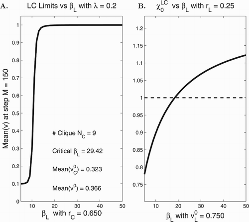
If we knew the connections in our network (the knowledge we assume for ${\chi }_0$ and ${\chi }_0^{SF}$) as well as the influence which includes the weights of the connections, we could compute the following parameter: ${\chi }_0^{LC}=\frac{({\beta }_L{v}_L^0+N_C{\overline{v}}_C^0)/({\beta }_L+N_C)}{(r_L+N_C{r}_C)/(N_C+1)}$ whose values, as they depend on ${\beta }_L$, are plotted in Figure 2(B). Observe that the point (in ${\beta }_L$) where ${\chi }_0^{LC}=1$ (where ${\beta }_L\cong 18$) is an accurate predictor of the emergence of heavy drinking (Figure 2(B) – members $v_i$-index getting close to 1).

3. Simulations

In this section we extend the ${\chi }_0$ analysis developed in Theorems 2.2–2.3 to general graphs using computer experimentation. We have developed MATLAB codes that create either random or scale-free networks with N nodes and then implement either the cubic or switch network models for M steps.

For these simulations a symmetric adjacency matrix W was generated where each entry $w_{ij}$ is 0 or 1 depending on whether there is a connection between nodes (individuals) i and j. Thus, ${\mathcal{N}}_i$ is just the nonzeroes in row i, $|{\mathcal{N}}_i|$ is the number of nonzeroes in that row and the ${\sigma }_{ij}=1/|{\mathcal{N}}_i|$ if $w_{ij}=1$.

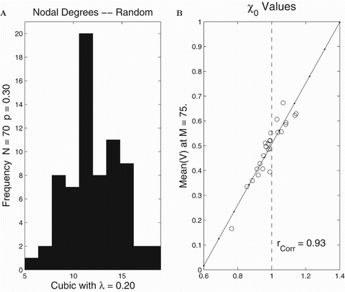
Figure 3 has our results for many runs on a fixed random network with the cubic model in order to assess how well the ${\chi }_0$-criterion derived in Theorem 2.2 predicts actual behaviour. The initial conditions and resiliences are randomly chosen for each run and uniformly distributed on $[0,1]$. We find that ${\chi }_0={\overline{v}}^0/\overline{r}$ is well correlated with the final averages for the index $\overline{v}$ at end step M in the case of this random network (correlation $r_{Corr}\cong 0.93$).

Figure 3. Computational assessment of ${\chi }_0$ in the case of random networks with the cubic model. There were 25 runs on a fixed random network with N=70 nodes assembled with connection probability p=0.3 and the degree distribution in (A). The set of final means $\overline{v}$ at $M=75$ steps versus ${\chi }_0$ values on the horizontal axis are shown in (B). The $r_i$ and $v_i^0$'s were uniformly distributed. The least squares line ${\overline{v}}^M$ vs ${\chi }_0$ is provided in (B) with correlation value r.

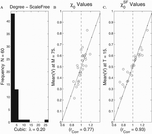
In Figure 4 we display results from computer runs on a scale-free network with the cubic model. Here, we find that ${\chi }_0={\overline{v}}^0/\overline{r}$ is not a good predictor of spread (correlation $r_{Corr}\cong 0.77$). However, if we use ${\chi }_0^{SF}$ then we typically find a better correlation ($r_{Corr}=0.93$).

Figure 4. Computational assessment of ${\chi }_0$ and ${\chi }_0^{SF}$ in the case of scale-free networks with the cubic model. There were 25 runs on a scale-free network with the nodal connection distribution in (A) and N=70 nodes. The set of final means $\overline{v}$ at M=75 steps versus ${\chi }_0$ are shown in (B) and versus ${\chi }_0^{SF}$ in (C). The $r_i$ and $v_i^0$'s were uniformly distributed. The least squares lines are provided in (B) and (C).

In Figure 5 we continue the investigations whose results we showed in Figures 3 and 4. In Figure 5(A), we show how the correlation between ${\chi }_0$ and spread is enhanced as more and more connections are added to the random network.

Figure 5. More on computations to assess ${\chi }_0$ and ${\chi }_0^{SF}$. (A) Correlations of ${\chi }_0$ and ${\overline{v}}^M$ for random networks with varying connection fractions P. (B) Histogram of outcomes for 15 correlation computations with ${\chi }_0$. (C) Histogram of outcomes for 15 correlation computations with ${\chi }_0^{SF}$.

In Figures 5(B) and (C) we look at histograms of ${\chi }_0$ and ${\chi }_0^{SF}$ for scale-free networks that enhance the results observed in Figure 4. In each of these cases we did 15 experiments where each consisted of 25 runs on a particular fixed scale-free network. The results reinforced the predictability of ${\chi }_0^{SF}$ for such scale-free networks. Figure 4(B) has the correlation of ${\chi }_0$ and ${\overline{v}}^M$ as 0.737, while Figure 4(C) has the correlation of ${\chi }_0^{SF}$ and ${\overline{v}}^M$ as 0.908.

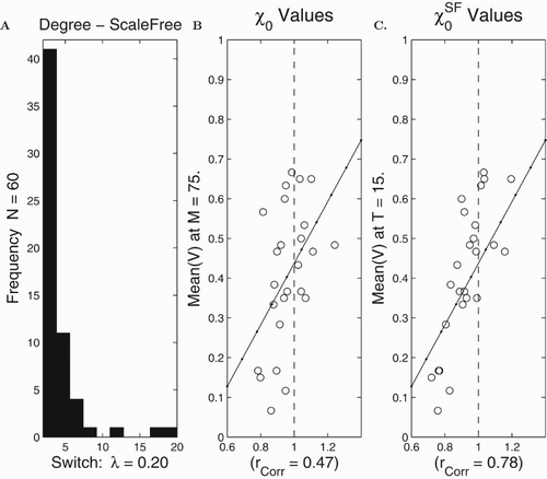
In Figure 6 we display results from computer runs on a scale-free network with the switch model. Here, we find that ${\chi }_0$ is again not a good predictor of spread (correlation $r_{Corr}\cong 0.47$). However, if we use ${\chi }_0^{SF}$ then we typically find a better correlation $r_{Corr}=0.78$. Unfortunately, the correlation between ${\chi }_0^{SF}$ is not as solid with the switch model as it was with the cubic.

Figure 6. Computational assessment of ${\chi }_0$ and ${\chi }_0^{SF}$ in the case of scale-free networks with the switch model. There were 25 runs on a scale-free network with the nodal connection distribution in (A) and N=70 nodes. The set of final means $\overline{v}$ at time T=15 are shown in (B) and (C). The $r_i$ and $v_i^0$'s were uniformly distributed. The least squares lines are provided in (B) and (C).

4. Applications – karate club and multiple clique networks

In this section we investigate the accuracy of ${\chi }_0$ and ${\chi }_0^{SF}$ for our cubic model on the spread of heavy drinking for two example networks.

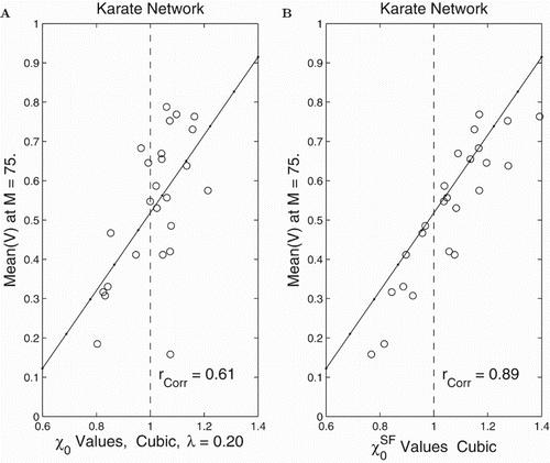
In the karate club [27] there are two leaders who are not on friendly terms. In Figure 7 we display the network and its degree distribution. In Figure 8 we provide our results from applying our cubic model on this application network. The results in Figure 8 where the correlation to ${\chi }_0^{SF}$ is much better than to ${\chi }_0$ was typical of our computations. The karate network has two hubs which suggest it is closer to a scale-free network than a random network. The computations show ${\chi }_0^{SF}$ is a better predictor of spread than ${\chi }_0$ which is consistent with our new ideas. The correlation between predicted ${\chi }_0^{SF}$ values and outcomes was 0.89 while it was only 0.61 for ${\chi }_0$.

Figure 7. The karate club network. (A) Visualization of the nodes and connections. (B) The degree distribution – number of connections for each node.

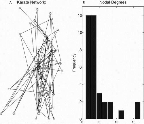
Figure 8. Computational assessment of ${\chi }_0$ and ${\chi }_0^{SF}$ (see (5(5) ${\chi }_0=\frac{{\overline{v}}^0}{\overline{r}},{\chi }_0^{SF}=\frac{\sum _{i=1}^N{\mathrm{deg}}_i\cdot v_i^0}{\sum _{i=1}^N{\mathrm{deg}}_i\cdot r_i}\text{where}{\mathrm{deg}}_i=|{\mathcal{N}}_i|\text{and}{\overline{v}}^0=\sum _{i=1}^N{v}_i^0.$(5) )) for the Cubic Model on the karate network. There were 25 simulations with sets of $r_i$'s chosen randomly for each. Circles correspond to mean values $\overline{v}$ after 75 steps. Also shown are the least squares fit lines with horizontal coordinate ${\chi }_0$ for (A) and ${\chi }_0^{SF}$ for (B).

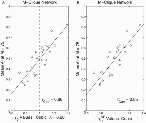
We also considered a multiple clique network as displayed in Figure 9(A). In this case there are several individuals who know members outside their own clique as well as others who only have friends (connections) within their clique. In our computations we found that both the ${\chi }_0$ and ${\chi }_0^{SF}$ quantities are good predictors for the multiple clique network (see Figures 9 and 10). Here, the correlation between final outcomes for drinking $\overline{v}$ and ${\chi }_0$ was 0.86 and was 0.81 for ${\chi }_0^{SF}$.

Figure 9. The multiple clique network. (A) Visualization of the nodes and connections. (B) The degree distribution – number of connections for each node.

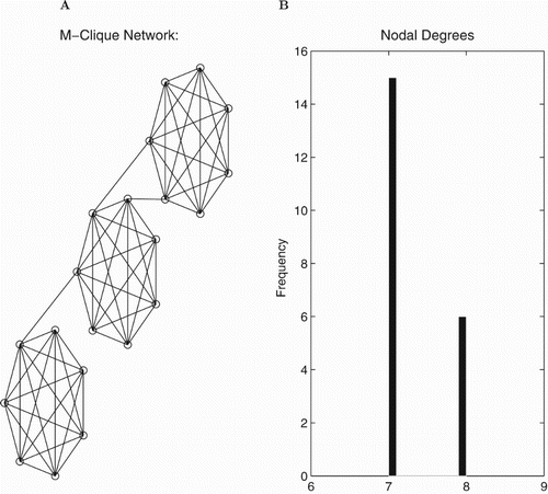
Figure 10. Computational assessment of ${\chi }_0$ and ${\chi }_0^{SF}$ (see (5(5) ${\chi }_0=\frac{{\overline{v}}^0}{\overline{r}},{\chi }_0^{SF}=\frac{\sum _{i=1}^N{\mathrm{deg}}_i\cdot v_i^0}{\sum _{i=1}^N{\mathrm{deg}}_i\cdot r_i}\text{where}{\mathrm{deg}}_i=|{\mathcal{N}}_i|\text{and}{\overline{v}}^0=\sum _{i=1}^N{v}_i^0.$(5) )) for the Cubic Model on the Multiple Clique Network. There were 25 simulations with $r_i$'s chosen randomly for each. Circles correspond to mean values $\overline{v}$ after 75 steps. Also shown are the least squares fit lines with horizontal coordinate ${\chi }_0$ for (A) and ${\chi }_0^{SF}$ for (B).

5. Discussion

In this paper we have examined two related simple difference models (cubic and switch) for the spread of alcohol abuse on networks. Each node or individual i in the network is identified by their drinking index $v_i^m\in [0,1]$ at each time step m.

Inspired by the idea of reproduction number or $R_0$ in disease spread, we investigated three parameters ${\chi }_0$, ${\chi }_0^{SF}$ and ${\chi }_0^{LC}$ that depended on initial members drinking levels, resiliences and, for the latter two, connections and influence. We found that ${\chi }_0$ was a good predictor of behaviour for the all-to-all and random networks. The ${\chi }_0^{SF}$ and ${\chi }_0^{LC}$ were better predictors for the behaviour of networks where the influence of individual nodes can be vastly different either through connections or weights.

In the future we intend to investigate treatment programmes such as alcoholics anonymous with our models. We find the question of finding optimum interventions for given networks and initial connection schemes very appealing and would look to [14,15] for inspiration.

Acknowledgments

The basic idea for this paper and specifically the cubic model was introduced in a Mathematical Problems in Industry workshop [26]. The first author is grateful to Richard Braun for introducing him to their work. In this paper we have added scale-free networks, the switch model and analysis of specialized small networks (all-to-all, star and leader clique).

Disclosure statement

No potential conflict of interest was reported by the authors.

Additional information

Funding

The first author is grateful to the Mathematical Biosciences Institute for their hospitality and the introduction to his other collaborators. In that regard, this research has been supported in part by the Mathematical Biosciences Institute, Ohio State University and is funded by National Science Foundation under grants DMS 0931642 and DMS 1440386.

References

- R. Bani, R. Hameed, S. Szymanowski, P. Greenwood, C. Kribs-Zaleta, and A. Mubayi, Influence of environmental factors on college alcohol drinking patterns, Math. Biosci. Eng. 10 (2013), pp. 1281–1300.
- A.-L. Barabasi, Linked, Perseus, 2002.
- A. Barrat, M. Barthelemy, and A. Vespignani, Dynamical Processes on Complex Networks, Cambridge University Press, Canmbridge, 2008.
- B. Benedict, Modeling alcoholism as a contagious disease: How ‘infected’ drinking buddies spread problem drinking, SIAM News 40 (2007), 3 pages.
- R.J. Braun, R.A. Wilson, J.A. Pelesko, J.R. Buchanan, and J.P. Gleeson, Applications of small world network theory in alcohol epidemiology, J. Alcohol Stud. 67 (2006), pp. 591–599.
- R. Braun, D.A French, Z. Teymuorglu, and T. Lewis, Continuum models of the spread of alcoholism, J. Integral Equations Appl. 22 (2010), pp. 441–462.
- A. Cintron-Arias, F. Sanchez, X. Wang, C. Castillo-Chavez, D.M. Gorman, and P.J. Gruenewald, The role of nonlinear relapse on contagion amongst drinking communities, in Mathematical and Statistical Estimation Approaches in Epidemiology, G. Chowel, J.M. Hayman, L.M.A. Bettencourt, and P.C. Castillo-Chavez, eds., 2009, Springer, New York, pp. 343–360.
- D. Easley and J. Kleinberg, Networks, Crowds and Markets, University Press, Cambridge, 2010.
- M. Golubitsky and I. Stewart, Nonlinear dynamics of networks: The groupoid formalism, Bull. Am. Math. Soc. 43 (2006), pp. 305–365.
- D.M. Gorman, J. Mezic, I. Mezic, and P.J. Gruenwald, Agent-based modeling of drinking behavior: A preliminary model and potential applications to theory and practice, Am. J. Public Health 96 (2006), pp. 2055–2060.
- D.B. Kandel, Drug and drinking behavior among youth, Ann. Rev. Sociol. 6 (1980), pp. 235–285.
- D.B. Kandel, On processes of peer influences in adolescent drug use: A developmental perspective, Adv. Alcohol Substance Abuse 3–4 (1985), pp. 139–162.
- E. Kuntsche, R. Knibbe, G. Gmel, and R. Engels, Why do young people drink? A review of drinking motives, Clin. Psychol. Rev. 25 (2005), pp. 841–861.
- R. Leander, S. Lenhardt, and V. Protopopescu, Using optimal control theory to identify network structures that foster synchrony, Phys. D 241 (2012), pp. 574–582.
- S. Lenhart and J.T. Workman, Optimal Control Applied to Biological Models, Chapman and Hall/CRC Press, Boca Raton, 2007.
- J.L. Manthey, A.Y. Aidoo, and K.Y. Ward, Campus drinking: An epidemiological model, J. Biol. Dyn. 2 (2008), pp. 346–356.
- A. Mubayi, P. Greenwood, C. Castillo-Chavez, P. Grunewald, and D.M. Gorman, The impact of relative residence times on the distribution of heavy drinkers in highly distinct environments, Socio-Econ. Plan. Sci. XX (2008), pp. 1–12.
- A. Mubayi, P. Greenwood, X. Wang, C. Castillo-Chavez, D.M. Gorman, P. Gruenewald, and R.F. Salt, Types of drinkers and drinking settings: An application of a mathematical model, Addiction 106 (2010), pp. 749–758.
- G. Mulone and B. Straughan, Modeling binge drinking, Int. J. Biomath. 5 (2012), pp. 57–70.
- M.E.J. Newman, The structure and function of complex networks, SIAM Rev. 45 (2003), pp. 167–256.
- J.S. Rasul, R.G. Rommel, G.M. Jacquez, B.G. Fitzpatrick, A.S. Ackleh, N. Simonsen, and R.A. Scribner, Heavy episodic drinking on college campuses: Does changing the drinking age make a difference?, J. Stud. Alcohol Drugs 72 (2011), pp. 15–23.
- Results from the 2012 National Survey on Drug Use and Health: Summary of National Findings, 2013.
- J.N. Rosenquist, J. Murabito, J.H. Fowler, and N. Christakis, The spread of alcohol consumption behavior in a large social network, Ann. Internal Med. 152 (2010), pp. 426–433.
- F. Sanchez, X. Wang, C. Castillo-Chavez, D.M. Gorman, and P.G. Gruenewald, Drinking as an epidemic: A simple mathematical model with recovery and relapse, in Guide to Evidence Based Relapse Prevention, K. Witkiewitz, G.A. Marlatt, eds., Academic Press, New York, 2007, pp. 353–368.
- S.H. Strogatz, Exploring complex networks, Nature 410 (2001), pp. 268–276.
- R.A. Wilson, J.R. Buchanon, J. Gleeson, and R. Braun, A network model of alcoholism and alcohol policy, Mathematical Problems in Industry Report (November 5, 2004).
- W.W. Zachary, An information flow model for conflict and fission in small groups, J. Anthropol. Res. 33 (1977), pp. 452–473.