Effects of pesticide dose on Holling II predator–prey model with feedback control

ABSTRACT

We establish a Holling II predator–prey system with pesticide dose response non-linear pulses and then study the global dynamics of the model. First, we construct the Poincaré map in the phase set and discuss its main properties. Second, threshold conditions for the existence and stability of boundary periodic solution and order-$k(k\ge 1)$ periodic solutions have been provided. The results show that the pesticide dose increases when the period of control increases, while it will decrease as threshold increases. Sensitivity analyses reveal that critical condition for the stability of boundary periodic solution is very sensitive to control parameters and pesticide doses. The bifurcation analysis reveals that the proposed model exists complex dynamics. Compared to the model with fixed moments, it demonstrates that the density of pest population not only can be controlled below the threshold but also can avoid some negative effects due to pesticide application, confirming the importance of biological control.

KEYWORDS:

• Dose response
• chemical control
• Poincaré map
• sensitivity analyses

1. Introduction

Chemical control is viewed as a classical method to control pests, which is usually realized by spraying insecticides. However, many pest populations have developed resistance to insecticide when chemical control is applied repeatedly [31]. Thereafter, insecticide will no longer be effective even if we increase the doses [8]. To overcome the problem of pest resistance and further control pest with resistance, integrated pest management (IPM) is proposed, which suggests that chemical control is implemented together with biological control [33]. Biological control is another important control strategy with aim of reducing number of pest populations by means of releasing natural enemies [24].

In order to determine the critical times or thresholds for IPM applications, we first need to know the interactions between predator and prey populations. It has been pointed out that Holling type II predator–prey system plays a significant role in describing the relations between the pest population and natural enemy population, which can be formulated by the following ordinary differential equations: (1) $\begin{array}{rl}\frac{\mathrm{d}x\left(t\right)}{\mathrm{d}t}& =rx\left(t\right)\left(1-\frac{x\left(t\right)}{K}\right)-\frac{ax\left(t\right)y\left(t\right)}{1+wx\left(t\right)},\\ \frac{\mathrm{d}y\left(t\right)}{\mathrm{d}t}& =\frac{cx\left(t\right)y\left(t\right)}{1+wx\left(t\right)}-\mathrm{d}y\left(t\right),\end{array}$(1) where $x\left(t\right)$ and $y\left(t\right)$ denote densities of the prey (pest) and predator (natural enemy) populations at time t. r is the intrinsic growth rate of the prey, K represents carrying capacity, $ax\left(t\right)/(1+wx(t\left)\right)$ indicates the Holling type II functional response, d is the death rate of the predator and c is the ratio of biomass conversion and satisfies 0<c<a. Kuang and Freedman pointed out that system (1(1) $\begin{array}{rl}\frac{\mathrm{d}x\left(t\right)}{\mathrm{d}t}& =rx\left(t\right)\left(1-\frac{x\left(t\right)}{K}\right)-\frac{ax\left(t\right)y\left(t\right)}{1+wx\left(t\right)},\\ \frac{\mathrm{d}y\left(t\right)}{\mathrm{d}t}& =\frac{cx\left(t\right)y\left(t\right)}{1+wx\left(t\right)}-\mathrm{d}y\left(t\right),\end{array}$(1) ) either exists a stable limit cycle or exists a stable positive equilibrium under certain conditions [10].

Based on system (1(1) $\begin{array}{rl}\frac{\mathrm{d}x\left(t\right)}{\mathrm{d}t}& =rx\left(t\right)\left(1-\frac{x\left(t\right)}{K}\right)-\frac{ax\left(t\right)y\left(t\right)}{1+wx\left(t\right)},\\ \frac{\mathrm{d}y\left(t\right)}{\mathrm{d}t}& =\frac{cx\left(t\right)y\left(t\right)}{1+wx\left(t\right)}-\mathrm{d}y\left(t\right),\end{array}$(1) ), many pulsed mathematical models with IPM have been proposed and analysed. Liu and coauthors constructed a pulsed model (1(1) $\begin{array}{rl}\frac{\mathrm{d}x\left(t\right)}{\mathrm{d}t}& =rx\left(t\right)\left(1-\frac{x\left(t\right)}{K}\right)-\frac{ax\left(t\right)y\left(t\right)}{1+wx\left(t\right)},\\ \frac{\mathrm{d}y\left(t\right)}{\mathrm{d}t}& =\frac{cx\left(t\right)y\left(t\right)}{1+wx\left(t\right)}-\mathrm{d}y\left(t\right),\end{array}$(1) ) with IPM applied at fixed moments, they investigated the existence and stability of pest-free periodic solution and proved that the proposed model is permanent, then bifurcation analysis with respect to the killing rate, releasing period and releasing amount was addressed [13,14]. In reality, IPM is often applied when pest number or density reaches the economic threshold (ET) rather than at fixed moments [7,25–27]. Thus the state-dependent feedback control, which provides a more reasonable description for IPM applications, is described by the impulsive semi-dynamical systems [4]. Thereafter, Liu and coauthors proposed model (1(1) $\begin{array}{rl}\frac{\mathrm{d}x\left(t\right)}{\mathrm{d}t}& =rx\left(t\right)\left(1-\frac{x\left(t\right)}{K}\right)-\frac{ax\left(t\right)y\left(t\right)}{1+wx\left(t\right)},\\ \frac{\mathrm{d}y\left(t\right)}{\mathrm{d}t}& =\frac{cx\left(t\right)y\left(t\right)}{1+wx\left(t\right)}-\mathrm{d}y\left(t\right),\end{array}$(1) ) with state-dependent feedback control. They studied the existence and stability of order-1 and order-2 periodic solutions, the results showed that the pests and enemies could stabilize along periodic solutions when the killing rate and releasing amount satisfied certain conditions. These studies were based on the assumptions that the killing rates of chemical control are constants.

Recently, Yang and Qin extended the impulsive model by considering the effect of resource limitation as non-linear pulse [21,35]. They not only showed that system (1(1) $\begin{array}{rl}\frac{\mathrm{d}x\left(t\right)}{\mathrm{d}t}& =rx\left(t\right)\left(1-\frac{x\left(t\right)}{K}\right)-\frac{ax\left(t\right)y\left(t\right)}{1+wx\left(t\right)},\\ \frac{\mathrm{d}y\left(t\right)}{\mathrm{d}t}& =\frac{cx\left(t\right)y\left(t\right)}{1+wx\left(t\right)}-\mathrm{d}y\left(t\right),\end{array}$(1) ) with pulsed control has periodic solutions with any period but also indicated that resource limitation has great influence on successful pest control. In addition, Liang and coauthors proposed and investigated impulsive pest-natural enemy models with evolution of pesticide resistance as non-linear pulses [12]. In these studies, non-linear pulses were introduced to assess how killing rates caused by insecticide affect the outbreaks of pest population. However, none of the models incorporate the effects of pesticide doses (i.e. dose response) into the classical model (1(1) $\begin{array}{rl}\frac{\mathrm{d}x\left(t\right)}{\mathrm{d}t}& =rx\left(t\right)\left(1-\frac{x\left(t\right)}{K}\right)-\frac{ax\left(t\right)y\left(t\right)}{1+wx\left(t\right)},\\ \frac{\mathrm{d}y\left(t\right)}{\mathrm{d}t}& =\frac{cx\left(t\right)y\left(t\right)}{1+wx\left(t\right)}-\mathrm{d}y\left(t\right),\end{array}$(1) ) with pulse control, and this raises several questions: (1) What is the relationship among doses, the releasing period and threshold ET? (2) How do control parameters including doses, releasing period and ET affect the successful pest control? (3) How do insecticide doses affect the dynamics of the proposed impulsive predator–prey system? To conquer these questions, we develop novel impulsive model (1(1) $\begin{array}{rl}\frac{\mathrm{d}x\left(t\right)}{\mathrm{d}t}& =rx\left(t\right)\left(1-\frac{x\left(t\right)}{K}\right)-\frac{ax\left(t\right)y\left(t\right)}{1+wx\left(t\right)},\\ \frac{\mathrm{d}y\left(t\right)}{\mathrm{d}t}& =\frac{cx\left(t\right)y\left(t\right)}{1+wx\left(t\right)}-\mathrm{d}y\left(t\right),\end{array}$(1) ) concerning the effects of doses of chemical control by introducing state-dependent feedback control, which are formulated by the following system: (2) $\left\{\begin{array}{l}\left.\begin{array}{l}\frac{\mathrm{d}x\left(t\right)}{\mathrm{d}t}=rx\left(t\right)\left(1-\frac{x\left(t\right)}{K}\right)-\frac{ax\left(t\right)y\left(t\right)}{1+wx\left(t\right)}\\ \frac{\mathrm{d}y\left(t\right)}{\mathrm{d}t}=\frac{cx\left(t\right)y\left(t\right)}{1+wx\left(t\right)}-\mathrm{d}y\left(t\right)\end{array}\right\}x\left(t\right)<ET,\\ \left.\begin{array}{l}x\left(t^{+}\right)=S_1\left(D\right)x\left(t\right)\\ y\left(t^{+}\right)=S_2\left(D\right)y\left(t\right)+\tau \end{array}\right\}x\left(t\right)=ET,\end{array}\right.$(2) where $S_1\left(D\right)$ and $S_2\left(D\right)$ represent survival fractions of prey and predator populations when a given dose D of insecticides is applied, and $0\le S_1\left(D\right),S_2\left(D\right)\le 1$. We assume that insecticide kills both of prey and predator populations, but that the killing rates differ for both populations, with the response curves in all cases given by the exponential functions $S_1\left(D\right)={\mathrm{e}}^{-k_{1}D}$, and $S_2\left(D\right)={\mathrm{e}}^{-k_{2}D}$ [20], and $0\le k_i\le 1(i=1,2)$ denote the pharmacokinetics of insecticide. $\tau >0$ is the release amount of the predator when a dose D of insecticide was sprayed. We denote $x\left(0^{+}\right)$ and $y\left(0^{+}\right)$ as the initial densities of prey and predator populations. From biological significance, the initial density of prey is assumed to be less than the given threshold ET. As the density of prey grows, the threshold ET will finally be reached at time t. Thereby, a given dose D of pesticide will be sprayed and a certain amount τ of predators will then be released in order to control the prey, and consequently the amounts of prey and predator are updated to ${\mathrm{e}}^{-k_{1}D}ET$ and ${\mathrm{e}}^{-k_{2}D}y\left(t\right)+\tau$, respectively.

The rest of paper is arranged as follows: the useful definitions and important lemmas about the impulsive semi-dynamical systems can be found in Section 2. In Section 3, we will first deduce the expression of the Poincaré map and then give its main properties. In Section 4, we mainly prove the existence of boundary periodic solution and order-$k(k\ge 1)$ periodic solutions. In Section 5, numerical results including sensitivity analyses and bifurcation analyses are carried out, and biological implications about the pest control are addressed. At last, a conclusion is presented.

2. Preliminaries

The generalized planar impulsive semi-dynamical systems can be defined by the following system [1,22]: (3) $\left\{\begin{array}{l}\left.\begin{array}{l}\frac{\mathrm{d}x\left(t\right)}{\mathrm{d}t}=P(x,y)\\ \frac{\mathrm{d}y\left(t\right)}{\mathrm{d}t}=Q(x,y)\end{array}\right\}(x,y)\notin \mathcal{I},\\ \left.\begin{array}{l}{x}^{+}=x+\alpha (x,y)\\ y^{+}=y+\beta (x,y)\end{array}\right\}(x,y)\in \mathcal{I},\end{array}\right.$(3) where $(x,y)\in R^2$, let $x^{+}=x\left(t^{+}\right)$ and $y^{+}=y\left(t^{+}\right)$, and $P,Q,\alpha ,\beta$ are continuous functions from $R^2$ to R. Let $\mathcal{I}\subset R^2$ be impulsive set. For any $z(x,y)\in \mathcal{I}$, the map $I:R^2⟶R^2$ is defined as $z^{+}=I\left(z\right)=(x+\alpha (x,y),y+\beta (x,y\left)\right)=(x^{+},y^{+})\in R^2,$ and $z^{+}$ is denoted as impulsive point of z.

We denote $\mathcal{P}=I\left(\mathcal{I}\right)$ as phase set (i.e. for any $z\in \mathcal{I},I\left(z\right)=z^{+}\in \mathcal{P}$), and $\mathcal{P}\cap \mathcal{I}=\text{Ø}$. Let X be a metric space and $R_{+}$ be set of all non-negative reals, then we call $(X,\mathrm{\Pi },R)$ or $(X,\mathrm{\Pi })$ as a semi-dynamical system. For any $z\in X$, the function ${\mathrm{\Pi }}_z:R⟶X$ defined by ${\mathrm{\Pi }}_z\left(t\right)=\mathrm{\Pi }(z,t)$ is clearly continuous such that $\mathrm{\Pi }(z,0)=z$ for all $z\in X$, and $\mathrm{\Pi }\left(\mathrm{\Pi }\right(z,t),s)=\mathrm{\Pi }(z,t+s)$ for all $z\in X$ and $t,s\in R_{+}$. $G(z,t)=\{w\in X|\mathrm{\Pi }(w,t)=z\}$ is the attainable set of z at $t\in R_{+}$ and let $\mathcal{I}\left(z\right)={\mathcal{I}}^{+}\left(z\right)\cup {\mathcal{I}}^{-}\left(z\right)$. Based on these notations, we introduce some Definitions and Lemmas [3,9].

Definition 2.1

An impulsive semi-dynamical system $(X,\mathrm{\Pi };\mathcal{I},I)$ consists of a continuous semi-dynamical system $(X,\mathrm{\Pi })$ together with a non-empty closed subset $\mathcal{I}$ (or impulsive set) of X and a continuous function $I:\mathcal{I}⟶X$ such that the following property holds. No point $z\in X$ is a limit point of $\mathcal{I}\left(z\right)$; $\left\{t|G\right(z,t)\cap \mathcal{I}\ne \text{Ø}\}$ is a closed subset of R.

Definition 2.2

A trajectory ${\mathrm{\Pi }}_z$ in $(X,\mathrm{\Pi },\mathcal{I},I)$ is said to be periodic of period $T_k$ and order k if there exist non-negative integers $m\ge 0$ and $k\ge 1$ such that k is the smallest integer for which $z_m^{+}=z_{m+k}^{+}$ and $T_k=\sum _{i=m}^{m+k-1}\mathrm{\Phi }\left(z_i\right)=\sum _{i=m}^{m+k-1}{s}_i$.

Lemma 2.3

[1,22] The T-periodic solution $(x,y)=\left(\xi \right(t),\eta (t\left)\right)$ of system (4) $\begin{array}{rl}\frac{\mathrm{d}x}{\mathrm{d}t}& =P(x,y),\frac{\mathrm{d}y}{\mathrm{d}t}=Q(x,y),\mathrm{if}\phi (x,y)\ne 0,\\ x^{+}& =x+\alpha (x,y),y^{+}=y+\beta (x,y),\mathrm{if}\phi (x,y)=0,\end{array}$(4) is orbitally asymptotically stable and enjoys the property of asymptotic phase if the Floquet multiplier ${\mu }_2$ satisfies the condition $|{\mu }_2|<1,$ where ${\mu }_2=\prod _{k=1}^q{\mathrm{\Delta }}_k\exp \left({\int }_0^T\left[\frac{\mathrm{\partial }P}{\mathrm{\partial }x}\left(\xi \right(t),\eta (t\left)\right)+\frac{\mathrm{\partial }Q}{\mathrm{\partial }y}\left(\xi \right(t),\eta (t\left)\right)\right]\mathrm{d}t\right)$ with ${\mathrm{\Delta }}_k=\frac{P_{+}\left(\frac{\mathrm{\partial }\beta }{\mathrm{\partial }y}\frac{\mathrm{\partial }\phi }{\mathrm{\partial }x}-\frac{\mathrm{\partial }\beta }{\mathrm{\partial }x}\frac{\mathrm{\partial }\phi }{\mathrm{\partial }y}+\frac{\mathrm{\partial }\phi }{\mathrm{\partial }x}\right)+Q_{+}\left(\frac{\mathrm{\partial }\alpha }{\mathrm{\partial }x}\frac{\mathrm{\partial }\phi }{\mathrm{\partial }y}-\frac{\mathrm{\partial }\alpha }{\mathrm{\partial }y}\frac{\mathrm{\partial }\phi }{\mathrm{\partial }x}+\frac{\mathrm{\partial }\phi }{\mathrm{\partial }y}\right)}{P\frac{\mathrm{\partial }\phi }{\mathrm{\partial }x}+Q\frac{\mathrm{\partial }\phi }{\mathrm{\partial }y}},$ and φ is continuously differentiable with respect to x,y. $(x,y)\notin \mathcal{I}$ can also be denoted by $\phi (x,y)\ne 0$. $P,Q,\mathrm{\partial }\alpha /\mathrm{\partial }x,\mathrm{\partial }\alpha /\mathrm{\partial }y,\mathrm{\partial }\beta /\mathrm{\partial }x,\mathrm{\partial }\beta /\mathrm{\partial }y,\mathrm{\partial }\phi /\mathrm{\partial }x$ and $\mathrm{\partial }\phi /\mathrm{\partial }y$ are calculated at the point $\left(\xi \right(t_k),\eta (t_k\left)\right),$ $P_{+}=P\left(\xi \right(t_k^{+}),\eta (t_k^{+}\left)\right)$ and $Q_{+}=Q\left(\xi \right(t_k^{+}),\eta (t_k^{+}\left)\right).$ $t_k$ ($k,q\in N$, N is non-negative integers) is the time of the kth jump.

System (1(1) $\begin{array}{rl}\frac{\mathrm{d}x\left(t\right)}{\mathrm{d}t}& =rx\left(t\right)\left(1-\frac{x\left(t\right)}{K}\right)-\frac{ax\left(t\right)y\left(t\right)}{1+wx\left(t\right)},\\ \frac{\mathrm{d}y\left(t\right)}{\mathrm{d}t}& =\frac{cx\left(t\right)y\left(t\right)}{1+wx\left(t\right)}-\mathrm{d}y\left(t\right),\end{array}$(1) ) is the classical Holling II predator–prey system [10]. There are two isoclines denoted as $L_1$ and $L_2$, $L_1:x=\frac{d}{c-dw},L_2:y=\frac{r}{aK}(K-x)(1+wx).$ There are three equilibria for system (1(1) $\begin{array}{rl}\frac{\mathrm{d}x\left(t\right)}{\mathrm{d}t}& =rx\left(t\right)\left(1-\frac{x\left(t\right)}{K}\right)-\frac{ax\left(t\right)y\left(t\right)}{1+wx\left(t\right)},\\ \frac{\mathrm{d}y\left(t\right)}{\mathrm{d}t}& =\frac{cx\left(t\right)y\left(t\right)}{1+wx\left(t\right)}-\mathrm{d}y\left(t\right),\end{array}$(1) ), two boundary equilibria are $(0,0)$ and $E_0(K,0)$, the unique interior equilibrium $E^{\ast }(x^{\ast },y^{\ast })$ is positive provided $K(c-wd)-d>0$ with $x^{\ast }=d/(c-dw),y^{\ast }=\left(rc\right(K(c-wd)-d\left)\right)/\left(aK\right(c-wd{)}^2)$.

Lemma 2.4

1. If $K(c-wd)-d<0,$ then $E_0$ is globally stable.

2. If $x^{\ast }>(wK-1)/2w,$ then $E^{\ast }$ is a stable focus or node.

3. If $x^{\ast }\le (wK-1)/2w,$ then $E^{\ast }$ is unstable and system (1(1) $\begin{array}{rl}\frac{\mathrm{d}x\left(t\right)}{\mathrm{d}t}& =rx\left(t\right)\left(1-\frac{x\left(t\right)}{K}\right)-\frac{ax\left(t\right)y\left(t\right)}{1+wx\left(t\right)},\\ \frac{\mathrm{d}y\left(t\right)}{\mathrm{d}t}& =\frac{cx\left(t\right)y\left(t\right)}{1+wx\left(t\right)}-\mathrm{d}y\left(t\right),\end{array}$(1) ) exists a unique stable limit cycle.

The above Definitions and Lemmas play key roles in the rest of the paper. In reality, the pest population may reach the carrying capacity K if human actions are not applied. So we focus on the case (i) of Lemma 2.4 where $(0,0)$ is a saddle, $E_0$ is globally stable and all solution will finally tend to $E_0$. Thereby, ET<K holds naturally throughout the paper. The main objective of this paper is to investigate how the strength of control affects the outcomes of the pest control.

3. Poincaré map

3.1. The domains of the Poincaré map

The global dynamics of system (2(2) $\left\{\begin{array}{l}\left.\begin{array}{l}\frac{\mathrm{d}x\left(t\right)}{\mathrm{d}t}=rx\left(t\right)\left(1-\frac{x\left(t\right)}{K}\right)-\frac{ax\left(t\right)y\left(t\right)}{1+wx\left(t\right)}\\ \frac{\mathrm{d}y\left(t\right)}{\mathrm{d}t}=\frac{cx\left(t\right)y\left(t\right)}{1+wx\left(t\right)}-\mathrm{d}y\left(t\right)\end{array}\right\}x\left(t\right)<ET,\\ \left.\begin{array}{l}x\left(t^{+}\right)=S_1\left(D\right)x\left(t\right)\\ y\left(t^{+}\right)=S_2\left(D\right)y\left(t\right)+\tau \end{array}\right\}x\left(t\right)=ET,\end{array}\right.$(2) ) are not only influenced by the threshold ET but also determined by the survival fractions of prey and predator populations, because these two factors affect the domains of the impulsive and phase sets, in addition to the domains of the Poincaré map. While the existence of periodic solutions can be realized by discussing the fixed points of the Poincaré map. Therefore, the exact domains of the Poincaré map together with its main properties are needed to be investigated first.

The lines related to the impulsive and phase sets are defined by $L_3:x={\mathrm{e}}^{-k_{1}D}ET,L_4:x=ET.$

In view of 0<ET<K, the lines $L_3$ and $L_4$ always have intersect points with the line $L_2$. The unique intersect point of $L_2$ and $L_4$ is denoted as $Q(ET,y_Q)$, while the unique intersect point of $L_2$ and $L_3$ is denoted as $P({\mathrm{e}}^{-k_{1}D}ET,y_P)$, where $y_Q=\frac{r(K-ET)(1+wET)}{aK},y_P=\frac{r(K-{\mathrm{e}}^{-k_{1}D}ET)(1+w{\mathrm{e}}^{-k_{1}D}ET)}{aK}.$

Based on the definitions, system (2(2) $\left\{\begin{array}{l}\left.\begin{array}{l}\frac{\mathrm{d}x\left(t\right)}{\mathrm{d}t}=rx\left(t\right)\left(1-\frac{x\left(t\right)}{K}\right)-\frac{ax\left(t\right)y\left(t\right)}{1+wx\left(t\right)}\\ \frac{\mathrm{d}y\left(t\right)}{\mathrm{d}t}=\frac{cx\left(t\right)y\left(t\right)}{1+wx\left(t\right)}-\mathrm{d}y\left(t\right)\end{array}\right\}x\left(t\right)<ET,\\ \left.\begin{array}{l}x\left(t^{+}\right)=S_1\left(D\right)x\left(t\right)\\ y\left(t^{+}\right)=S_2\left(D\right)y\left(t\right)+\tau \end{array}\right\}x\left(t\right)=ET,\end{array}\right.$(2) ) defines an impulsive semi-dynamical system with $\alpha (x,y)=x({\mathrm{e}}^{-k_{1}D}-1),\beta (x,y)=y({\mathrm{e}}^{-k_{2}D}-1)+\tau ,$ the impulsive set is part of the line $L_4$, and $\mathcal{I}=\left\{(x,y)\in R^2\mid x=ET,0\le y\le \frac{r(K-ET)(1+wET)}{aK}\right\},$ while the continuous function takes the following expression: $I:(ET,y)\in \mathcal{I}⟶(x^{+},y^{+})=\left({\mathrm{e}}^{-k_{1}D}ET,{\mathrm{e}}^{-k_{2}D}y+\tau \right)\in R^2.$ Thus the phase set is $\mathcal{P}=I\left(\mathcal{I}\right)=\left\{(x^{+},y^{+})\in R^2\mid x^{+}={\mathrm{e}}^{-k_{1}D}ET,y^{+}\in D\right\}$ with $D=[\tau ,r{\mathrm{e}}^{-k_{2}D}(K-ET\left)\right(1+wET)/aK+\tau ]$. Without loss of generality, unless otherwise specified we assume that the initial point $(x_0^{+},y_0^{+})$ belongs to $\mathcal{P}$.

3.2. Poincaré map and its main properties

In the first quadrant, $L_3$ is chosen to define the Poincaré map. Since $E_0$ is globally stable, any trajectory initiating from point $H_k^{+}({\mathrm{e}}^{-k_{1}D}ET,y_k^{+})\in L_3$ must meet $L_4$ at a unique point $H_{k+1}(ET,y_{k+1})$. Owing to the Cauchy–Lipschitz Theorem, $y_{k+1}$ is only determined by $y_k^{+}$ and can be expressed by $y_{k+1}=g\left(y_k^{+}\right)$. Because $L_4$ contains part of the domain of impulsive set $\mathcal{I}$, point $H_{k+1}$ experiences one time pulse and then maps to $L_3$ at point $H_{k+1}^{+}({\mathrm{e}}^{-k_{1}D}ET,y_{k+1}^{+})$ with $y_{k+1}^{+}={\mathrm{e}}^{-k_{2}D}{y}_{k+1}+\tau$. Thus the Poincaré map can be defined by (5) $y_{i+1}^{+}={\mathrm{e}}^{-k_{2}D}g\left(y_i^{+}\right)+\tau \triangleq \varphi \left(y_i^{+}\right).$(5)

Now, we deduce the expression of the Poincaré map ϕ and then discuss its main properties. To do these, let $\begin{array}{rl}P\left(x\right(t),y(t\left)\right)& =rx\left(t\right)\left(1-\frac{x\left(t\right)}{K}\right)-\frac{ax\left(t\right)y\left(t\right)}{1+wx\left(t\right)},\\ Q\left(x\right(t),y(t\left)\right)& =\frac{cx\left(t\right)y\left(t\right)}{1+wx\left(t\right)}-\mathrm{d}y\left(t\right),\end{array}$ then model (2(2) $\left\{\begin{array}{l}\left.\begin{array}{l}\frac{\mathrm{d}x\left(t\right)}{\mathrm{d}t}=rx\left(t\right)\left(1-\frac{x\left(t\right)}{K}\right)-\frac{ax\left(t\right)y\left(t\right)}{1+wx\left(t\right)}\\ \frac{\mathrm{d}y\left(t\right)}{\mathrm{d}t}=\frac{cx\left(t\right)y\left(t\right)}{1+wx\left(t\right)}-\mathrm{d}y\left(t\right)\end{array}\right\}x\left(t\right)<ET,\\ \left.\begin{array}{l}x\left(t^{+}\right)=S_1\left(D\right)x\left(t\right)\\ y\left(t^{+}\right)=S_2\left(D\right)y\left(t\right)+\tau \end{array}\right\}x\left(t\right)=ET,\end{array}\right.$(2) ) can be rewritten as the following scalar differential equation: (6) $\begin{array}{rl}\frac{\mathrm{d}y}{\mathrm{d}x}& =\frac{\frac{cx\left(t\right)y\left(t\right)}{1+wx\left(t\right)}-\mathrm{d}y\left(t\right)}{rx\left(t\right)\left(1-\frac{x\left(t\right)}{K}\right)-\frac{ax\left(t\right)y\left(t\right)}{1+wx\left(t\right)}}\omega (x,y),\\ y\left({\mathrm{e}}^{-k_{1}D}ET\right)& =y_0^{+}.\end{array}$(6) Denote (7) $\mathrm{\Omega }=\left\{(x,y)\mid x>0,y>0,y<\frac{r(K-x)(1+wx)}{aK}\right\},$(7) it is clear that function $\omega (x,y)$ is continuously differentiable in Ω. Let $x_0^{+}={\mathrm{e}}^{-k_{1}D}ET$, $y_0^{+}S,S\in \mathcal{P}$ with $S<y_P$ which guarantees the initial point $(x_0^{+},y_0^{+})\in \mathrm{\Omega }$. Define $y\left(x\right)=y(x;{\mathrm{e}}^{-k_{1}D}ET,S)=y(x,S),{\mathrm{e}}^{-k_{1}D}ET\le x\le ET,$ and then model (6(6) $\begin{array}{rl}\frac{\mathrm{d}y}{\mathrm{d}x}& =\frac{\frac{cx\left(t\right)y\left(t\right)}{1+wx\left(t\right)}-\mathrm{d}y\left(t\right)}{rx\left(t\right)\left(1-\frac{x\left(t\right)}{K}\right)-\frac{ax\left(t\right)y\left(t\right)}{1+wx\left(t\right)}}\omega (x,y),\\ y\left({\mathrm{e}}^{-k_{1}D}ET\right)& =y_0^{+}.\end{array}$(6) ) gives (8) $y(x,S)=S+{\int }_{{\mathrm{e}}^{-k_{1}D}ET}^x\omega (s,y(s,S\left)\right)\mathrm{d}s.$(8) Concerning (5(5) $y_{i+1}^{+}={\mathrm{e}}^{-k_{2}D}g\left(y_i^{+}\right)+\tau \triangleq \varphi \left(y_i^{+}\right).$(5) ) and (8(8) $y(x,S)=S+{\int }_{{\mathrm{e}}^{-k_{1}D}ET}^x\omega (s,y(s,S\left)\right)\mathrm{d}s.$(8) ), the expression of the Poincaré map ϕ is (9) $\varphi \left(S\right)={\mathrm{e}}^{-k_{2}D}ETy(ET,S)+\tau .$(9)

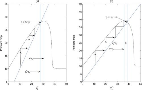
Theorem 3.1

The main properties of the Poincaré map ϕ are listed as follows (Figure 1):

1. The domain and range of ϕ are $[0,+\mathrm{\infty })$ and $[\tau ,\varphi (y_P\left)\right)=[\tau ,{\mathrm{e}}^{-k_{2}D}y({\mathrm{e}}^{-k_{1}D}ET,y_P)+\tau ],$ and further ϕ is increasing on $[0,y_P]$ and decreasing on $[y_P,+\mathrm{\infty })$.

2. ϕ is continuously differentiable in Ω.

3. ϕ is concave on $[0,y_P)$.

4. There always exists a unique fixed point for ϕ.

5. As $y_k^{+}\to +\mathrm{\infty },$ ϕ is bounded and exists a horizontal asymptote $\varphi =\tau$.

Figure 1. The Poincar$\acute{e}$ map ϕ related to the impulsive point series $y_k^{+}$ with parameters fixed as r=1.5, K=100, a=0.3, w=0.3, c=0.225, d=0.8, $k_1=0.5$, $k_2=0.3$, ET=35 and $\tau =10$. (a) D=0.8; (b) D=0.2.

Proof.

1. Since $E_0$ is globally stable, all solutions will finally arrive at $E_0$. So any solution starting from the phase set experiences pulses, and ϕ is defined on $[0,\mathrm{\infty })$. Choosing any two points with $y_i^{+},y_j^{+}\in [0,y_P]\subseteq L_3$, without loss of generality we assume that $y_i^{+}<y_j^{+}$, the Cauchy–Lipschitz Theorem implies that $y_{i+1}<y_{j+1}$ holds. After one single pulse, we obtain $\varphi \left(y_i^{+}\right)={\mathrm{e}}^{-k_{2}D}{y}_{i+1}+\tau <{\mathrm{e}}^{-k_{2}D}{y}_{j+1}+\tau =\varphi \left(y_j^{+}\right)$. Thus ϕ is increasing on $[0,y_P]$. By using the same methods, choosing two points $y_i^{+},y_j^{+}\in [y_P,+\mathrm{\infty })\subseteq L_3$ with $y_i^{+}<y_j^{+}$, the curves starting from these two points will first across the isocline $L_2$ and then arrive $L_3$ at points $({\mathrm{e}}^{-k_{1}D}ET,y_i^{\mathrm{\prime }})$ and $({\mathrm{e}}^{-k_{1}D}ET,y_j^{\mathrm{\prime }})$. In this case, the sign of the vector field has changed, it indicates that $y_i^{\mathrm{\prime }}>y_j^{\mathrm{\prime }}$. Soon afterwards these two curves meet $L_4$ at two points $(ET,y_{i+1})$ and $(ET,y_{j+1})$ with $y_{i+1}>y_{j+1}$. After one time pulse, one obtains $\varphi \left(y_i^{+}\right)={\mathrm{e}}^{-k_{2}D}{y}_{i+1}+\tau >{\mathrm{e}}^{-k_{2}D}{y}_{j+1}+\tau =\varphi \left(y_j^{+}\right).$ Therefore, on $[0,y_P]$ the map ϕ increases and on $[y_P,+\mathrm{\infty })$ the map ϕ decreases, and the range of ϕ is $[\tau ,{\mathrm{e}}^{-k_{2}D}y({\mathrm{e}}^{-k_{1}D}ET,y_P)+\tau ]$.

2. It is clear that $P(x,y)$ and $Q(x,y)$ are both continuous and differentiable in the first quadrant. In the light of the Cauchy–Lipschitz Theorem with parameters, ϕ is also continuously differentiable in Ω.

3. From (6(6) $\begin{array}{rl}\frac{\mathrm{d}y}{\mathrm{d}x}& =\frac{\frac{cx\left(t\right)y\left(t\right)}{1+wx\left(t\right)}-\mathrm{d}y\left(t\right)}{rx\left(t\right)\left(1-\frac{x\left(t\right)}{K}\right)-\frac{ax\left(t\right)y\left(t\right)}{1+wx\left(t\right)}}\omega (x,y),\\ y\left({\mathrm{e}}^{-k_{1}D}ET\right)& =y_0^{+}.\end{array}$(6) ), we have $\frac{\mathrm{\partial }\omega }{\mathrm{\partial }y}=\frac{rx\left(1-\frac{x}{K}\right)\left(\frac{cx}{1+wx}-d\right)}{{\left[rx\left(1-\frac{x}{K}\right)-\frac{axy}{1+wx}\right]}^2},\frac{{\mathrm{\partial }}^2\omega }{\mathrm{\partial }{y}^2}=\frac{2rx\left(1-\frac{x}{K}\right)\left(\frac{cx}{1+wx}-d\right)\frac{ax}{1+wx}}{{\left[rx\left(1-\frac{x}{K}\right)-\frac{axy}{1+wx}\right]}^3}.$ In the light of $x\le ET$, we have $rx\left(1-\frac{x}{K}\right)-\frac{axy}{1+wx}>0\text{and}\frac{cx}{1+wx}-d<0$ provided $0\le y<y_P$. It means that $\mathrm{\partial }\omega /\mathrm{\partial }y<0$ and ${\mathrm{\partial }}^2\omega /\mathrm{\partial }{y}^2<0$.

   For the scalar differential equation, it follows from Cauchy–Lipschitz Theorem with parameters that $\frac{\mathrm{\partial }y(x,S)}{\mathrm{\partial }S}=\exp \left[{\int }_{{\mathrm{e}}^{-k_{1}D}ET}^x\frac{\mathrm{\partial }}{\mathrm{\partial }y}\left(\frac{Q(z,y(z,S\left)\right)}{P(z,y(z,S\left)\right)}\right)\mathrm{d}z\right]>0$ and $\frac{{\mathrm{\partial }}^{2}y(x,S)}{\mathrm{\partial }{S}^2}=\frac{\mathrm{\partial }y(x,S)}{\mathrm{\partial }S}{\int }_{{\mathrm{e}}^{-k_{1}D}ET}^x\frac{{\mathrm{\partial }}^2}{\mathrm{\partial }{y}^2}\left(\frac{Q(z,y(z,S\left)\right)}{P(z,y(z,S\left)\right)}\right)\frac{\mathrm{\partial }y(x,S)}{\mathrm{\partial }S}\mathrm{d}z<0,$ which suggests that ϕ is concave on $[0,y_P)$ (Figure 1).

4. Since $\varphi \left(y\right)$ is increasing on $[0,y_P)$ and decreasing on $[y_P,+\mathrm{\infty })$, there are $y^1\in [0,y_P)$ and $y^2\in [y_P,+\mathrm{\infty })$ such that $\varphi \left(y^1\right)>y^1$ and $\varphi \left(y^2\right)<y^2$. If $\varphi \left(y_P\right)<y_P$, then the Poincaré map ϕ has at least a fixed point $y_f$ provided $\varphi \left(0\right)=\tau >0$, and $0<y_f<y_P$ (Figure 1a). Since ϕ is decreasing on $(y_P,+\mathrm{\infty })$, no other fixed point exists for all $y>y_P$. If $\varphi \left(y_P\right)\ge y_P$, then the Poincaré map ϕ has at least a fixed point $y_f$ provided $\varphi \left(y^2\right)<y^2$, and $y_P\le y_f<+\mathrm{\infty }$ (Figure 1b). Because ϕ is concave, so the fixed point $y_f$ of ϕ is unique.

5. Denote the closure of Ω by $\overline{\mathrm{\Omega }}=\left\{(x,y);x>0,y>0,y\le \frac{r(K-x)(1+wx)}{aK}\right\}.$ Under case (i), the $\overline{\mathrm{\Omega }}$ is an invariant set of system (2(2) $\left\{\begin{array}{l}\left.\begin{array}{l}\frac{\mathrm{d}x\left(t\right)}{\mathrm{d}t}=rx\left(t\right)\left(1-\frac{x\left(t\right)}{K}\right)-\frac{ax\left(t\right)y\left(t\right)}{1+wx\left(t\right)}\\ \frac{\mathrm{d}y\left(t\right)}{\mathrm{d}t}=\frac{cx\left(t\right)y\left(t\right)}{1+wx\left(t\right)}-\mathrm{d}y\left(t\right)\end{array}\right\}x\left(t\right)<ET,\\ \left.\begin{array}{l}x\left(t^{+}\right)=S_1\left(D\right)x\left(t\right)\\ y\left(t^{+}\right)=S_2\left(D\right)y\left(t\right)+\tau \end{array}\right\}x\left(t\right)=ET,\end{array}\right.$(2) ). In fact, let $L=y-\frac{r(K-x)(1+wx)}{aK}.$ If (10) ${\left[\left(P\right(x,y),Q(x,y\left)\right)\cdot \left(\frac{r}{a}\left(\frac{2wx+1}{K}-w\right),1\right)\right]}_{L=0}\le 0,$(10) where · is the scalar product of two vectors, then the vector field will finally enter into the boundary $\overline{\mathrm{\Omega }}$, which means that $\overline{\mathrm{\Omega }}$ is an invariant set. By calculation one obtains $\begin{array}{rl}V\left(x\right){\mid }_{L=0}& x\left(r\left(1-\frac{x}{K}\right)-\frac{ay}{1+wx}\right)\cdot \frac{r}{a}\left(\frac{2wx+1}{K}-w\right)+\left(\frac{cx}{1+wx}-d\right)y\\ & =\left(\frac{cx}{1+wx}-d\right)y<0.\end{array}$ Since ϕ is decreasing on $[y_P,+\mathrm{\infty })$ and increasing on $[0,y_P]$. Thus $\varphi \left(y_0^{+}\right)$ is bounded for any $y_0^{+}\in [0,y_P]$ and $\varphi \left(\right[y_P,+\mathrm{\infty }\left)\right)\subset \varphi \left(\right[0,y_P\left]\right)$. In addition, $\mathrm{d}y/\mathrm{d}t<0$ holds all along the line $L_3$ in the first quadrant. These lead to $\underset{y_k^{+}\to +\mathrm{\infty }}{lim}g\left(y_k^{+}\right)=0$ when $y_k^{+}\in D$. Furthermore, the trajectory initiating from $({\mathrm{e}}^{-k_{1}D}ET,0)$ meets the impulsive set at finite time, after one single pulse, we obtain $\underset{y_k^{+}\to +\mathrm{\infty }}{lim}\varphi \left(y_k^{+}\right)=\underset{y_k^{+}\to +\mathrm{\infty }}{lim}{\mathrm{e}}^{-k_{2}D}g\left(y_k^{+}\right)+\tau =\tau .$ All the results reveal that there is a horizontal asymptote $\varphi =\tau$ if $y_k^{+}\to +\mathrm{\infty }$ (Figure 1). This completes the proof.

4. Order-k periodic solutions

4.1. Boundary periodic solution of system (2)

For system (2(2) $\left\{\begin{array}{l}\left.\begin{array}{l}\frac{\mathrm{d}x\left(t\right)}{\mathrm{d}t}=rx\left(t\right)\left(1-\frac{x\left(t\right)}{K}\right)-\frac{ax\left(t\right)y\left(t\right)}{1+wx\left(t\right)}\\ \frac{\mathrm{d}y\left(t\right)}{\mathrm{d}t}=\frac{cx\left(t\right)y\left(t\right)}{1+wx\left(t\right)}-\mathrm{d}y\left(t\right)\end{array}\right\}x\left(t\right)<ET,\\ \left.\begin{array}{l}x\left(t^{+}\right)=S_1\left(D\right)x\left(t\right)\\ y\left(t^{+}\right)=S_2\left(D\right)y\left(t\right)+\tau \end{array}\right\}x\left(t\right)=ET,\end{array}\right.$(2) ), if predator population $y\left(t\right)$ goes to extinction and the release of predator is also terminated, then there is a boundary periodic solution of system (2(2) $\left\{\begin{array}{l}\left.\begin{array}{l}\frac{\mathrm{d}x\left(t\right)}{\mathrm{d}t}=rx\left(t\right)\left(1-\frac{x\left(t\right)}{K}\right)-\frac{ax\left(t\right)y\left(t\right)}{1+wx\left(t\right)}\\ \frac{\mathrm{d}y\left(t\right)}{\mathrm{d}t}=\frac{cx\left(t\right)y\left(t\right)}{1+wx\left(t\right)}-\mathrm{d}y\left(t\right)\end{array}\right\}x\left(t\right)<ET,\\ \left.\begin{array}{l}x\left(t^{+}\right)=S_1\left(D\right)x\left(t\right)\\ y\left(t^{+}\right)=S_2\left(D\right)y\left(t\right)+\tau \end{array}\right\}x\left(t\right)=ET,\end{array}\right.$(2) ). These lead to the following simple subsystem: (11) $\begin{array}{rl}\frac{\mathrm{d}x\left(t\right)}{\mathrm{d}t}& =rx\left(t\right)\left(1-\frac{x\left(t\right)}{K}\right),x\left(t\right)<ET,\\ x\left(t^{+}\right)& ={\mathrm{e}}^{-k_{1}D}x\left(t\right),x\left(t\right)=ET,\end{array}$(11) solving above equation with initial value $x\left(0^{+}\right)={\mathrm{e}}^{-k_{1}D}ET$, we obtain $x^{\mathrm{T}}\left(t\right)=\frac{{\mathrm{e}}^{-k_{1}D}ETK\exp \left(rt\right)}{K-{\mathrm{e}}^{-k_{1}D}ET+{\mathrm{e}}^{-k_{1}D}ET\exp \left(rt\right)},$ and the solution initiating from $\left(x^{\mathrm{T}}\right(t),0)$ will meet the line $L_4=ET$ with time T, so let $x^{\mathrm{T}}\left(T\right)=ET$ we have $ET=\frac{{\mathrm{e}}^{-k_{1}D}ETK\exp \left(rT\right)}{K-{\mathrm{e}}^{-k_{1}D}ET+{\mathrm{e}}^{-k_{1}D}ET\exp \left(rT\right)},$ solving it with respect to T and D, then $T=\frac{1}{r}\ln \frac{K-{\mathrm{e}}^{-k_{1}D}ET}{{\mathrm{e}}^{-k_{1}D}(K-ET)},D=\frac{1}{k_1}\ln \frac{ET+{\mathrm{e}}^{rT}(K-ET)}{K},$ where T represents the period of the boundary periodic solution, and D represents the insecticide dose needed to be sprayed in order to control the pest number below the threshold ET. Thereby, the boundary periodic solution of model (2(2) $\left\{\begin{array}{l}\left.\begin{array}{l}\frac{\mathrm{d}x\left(t\right)}{\mathrm{d}t}=rx\left(t\right)\left(1-\frac{x\left(t\right)}{K}\right)-\frac{ax\left(t\right)y\left(t\right)}{1+wx\left(t\right)}\\ \frac{\mathrm{d}y\left(t\right)}{\mathrm{d}t}=\frac{cx\left(t\right)y\left(t\right)}{1+wx\left(t\right)}-\mathrm{d}y\left(t\right)\end{array}\right\}x\left(t\right)<ET,\\ \left.\begin{array}{l}x\left(t^{+}\right)=S_1\left(D\right)x\left(t\right)\\ y\left(t^{+}\right)=S_2\left(D\right)y\left(t\right)+\tau \end{array}\right\}x\left(t\right)=ET,\end{array}\right.$(2) ) with period T gives (12) $\begin{array}{rl}{x}^{\mathrm{T}}\left(t\right)& =\frac{{\mathrm{e}}^{-k_{1}D}ETK\exp \left(r\right(t-(k-1)T\left)\right)}{K-{\mathrm{e}}^{-k_{1}D}ET+{\mathrm{e}}^{-k_{1}D}ET\exp \left(r\right(t-(k-1)T\left)\right)},\\ y^{\mathrm{T}}\left(t\right)& =0.\end{array}$(12)

Theorem 4.1

The boundary periodic solution $\left(x^{\mathrm{T}}\right(t),0)$ of system (2(2) $\left\{\begin{array}{l}\left.\begin{array}{l}\frac{\mathrm{d}x\left(t\right)}{\mathrm{d}t}=rx\left(t\right)\left(1-\frac{x\left(t\right)}{K}\right)-\frac{ax\left(t\right)y\left(t\right)}{1+wx\left(t\right)}\\ \frac{\mathrm{d}y\left(t\right)}{\mathrm{d}t}=\frac{cx\left(t\right)y\left(t\right)}{1+wx\left(t\right)}-\mathrm{d}y\left(t\right)\end{array}\right\}x\left(t\right)<ET,\\ \left.\begin{array}{l}x\left(t^{+}\right)=S_1\left(D\right)x\left(t\right)\\ y\left(t^{+}\right)=S_2\left(D\right)y\left(t\right)+\tau \end{array}\right\}x\left(t\right)=ET,\end{array}\right.$(2) ) is orbitally asymptotically stable provided (13) $R_0\triangleq \frac{d}{rD{k}_2}\ln \frac{{\mathrm{e}}^{-k_{1}D}(K-ET)}{K-{\mathrm{e}}^{-k_{1}D}ET}+\frac{cK}{rD{k}_2{k}_1(1+wK)}\ln \frac{(1+wET)(K-{\mathrm{e}}^{-k_{1}D}ET)}{(K-ET)(1+wET{\mathrm{e}}^{-k_{1}D})}<1.$(13)

Proof.

It follows from Lemma 2.3 that we obtain $\begin{array}{rl}P(x,y)& =rx\left(1-\frac{x}{K}\right)-\frac{axy}{1+wx},Q(x,y)=\frac{cxy}{1+wx}-\mathrm{d}y,\\ \alpha (x,y)& =x({\mathrm{e}}^{-k_{1}D}-1),\beta (x,y)=y({\mathrm{e}}^{-k_{2}D}-1)+\tau ,\phi (x,y)=x-ET,\\ \left(x^{\mathrm{T}}\right(T),y^{\mathrm{T}}(T\left)\right)& =(ET,0),\left(x^{\mathrm{T}}\right(T^{+}),y^{\mathrm{T}}(T^{+}\left)\right)=\left({\mathrm{e}}^{-k_{1}D}ET,0\right).\end{array}$ The derivations of the above formulas are $\begin{array}{rl}\frac{\mathrm{\partial }P}{\mathrm{\partial }x}& =r-\frac{2rx}{K}-\frac{ay}{(1+wx{)}^2},\frac{\mathrm{\partial }Q}{\mathrm{\partial }y}=\frac{cx}{1+wx}-d,\\ \frac{\mathrm{\partial }\alpha }{\mathrm{\partial }x}& ={\mathrm{e}}^{-k_{1}D}-1,\frac{\mathrm{\partial }\beta }{\mathrm{\partial }y}={\mathrm{e}}^{-k_{2}D}-1,\\ \frac{\mathrm{\partial }\phi }{\mathrm{\partial }x}& =1,\frac{\mathrm{\partial }\alpha }{\mathrm{\partial }y}=\frac{\mathrm{\partial }\beta }{\mathrm{\partial }x}=\frac{\mathrm{\partial }\phi }{\mathrm{\partial }y}=0,\end{array}$ so $\begin{array}{rl}{\mathrm{\Delta }}_1& =\frac{P_{+}(\frac{\mathrm{\partial }\beta }{\mathrm{\partial }y}\frac{\mathrm{\partial }\phi }{\mathrm{\partial }x}-\frac{\mathrm{\partial }\beta }{\mathrm{\partial }x}\frac{\mathrm{\partial }\phi }{\mathrm{\partial }y}+\frac{\mathrm{\partial }\phi }{\mathrm{\partial }x})+Q_{+}(\frac{\mathrm{\partial }\alpha }{\mathrm{\partial }x}\frac{\mathrm{\partial }\phi }{\mathrm{\partial }y}-\frac{\mathrm{\partial }\alpha }{\mathrm{\partial }y}\frac{\mathrm{\partial }\phi }{\mathrm{\partial }x}+\frac{\mathrm{\partial }\phi }{\mathrm{\partial }y})}{P\frac{\mathrm{\partial }\phi }{\mathrm{\partial }x}+Q\frac{\mathrm{\partial }\phi }{\mathrm{\partial }y}}\\ & =\frac{P^{+}\left(x^{\mathrm{T}}\right(T^{+}),y^{\mathrm{T}}(T^{+}\left)\right)(1+\frac{\mathrm{\partial }\beta }{\mathrm{\partial }y})}{P\left(x^{\mathrm{T}}\right(T),y^{\mathrm{T}}(T\left)\right)}=\frac{{\mathrm{e}}^{-k_{2}D}{\mathrm{e}}^{-k_{1}D}(K-{\mathrm{e}}^{-k_{1}D}ET)}{K-ET}.\end{array}$ Moreover, $\begin{array}{rl}& \exp \left({\int }_0^{\mathrm{T}}\left[\frac{\mathrm{\partial }P}{\mathrm{\partial }x}\left(x^{\mathrm{T}}\right(t),y^{\mathrm{T}}(t\left)\right)+\frac{\mathrm{\partial }Q}{\mathrm{\partial }y}\left(x^{\mathrm{T}}\right(t),y^{\mathrm{T}}(t\left)\right)\right]\mathrm{d}t\right)\\ & =\exp \left({\int }_0^{\mathrm{T}}\left[r-d-\frac{2r{x}^{\mathrm{T}}\left(t\right)}{K}+\frac{c{x}^{\mathrm{T}}\left(t\right)}{1+w{x}^{\mathrm{T}}\left(t\right)}\right]\mathrm{d}t\right)\\ & ={\left(\frac{K-{\mathrm{e}}^{-k_{1}D}ET}{{\mathrm{e}}^{-k_{1}D}(K-ET)}\right)}^{(r-d)/r}{\left(\frac{K-ET}{K-{\mathrm{e}}^{-k_{1}D}ET}\right)}^2\\ & \times {\left(\frac{(1+wET)(K-{\mathrm{e}}^{-k_{1}D}ET)}{(K-ET)(1+wET{\mathrm{e}}^{-k_{1}D})}\right)}^{cK/(1+wK)r}.\end{array}$ Then the explicit expression of Floquet multiplier ${\mu }_2$ is (14) $\begin{array}{rl}{\mu }_2& ={\mathrm{\Delta }}_1\exp \left({\int }_0^{\mathrm{T}}\left[\frac{\mathrm{\partial }P}{\mathrm{\partial }x}\left(x^{\mathrm{T}}\right(t),y^{\mathrm{T}}(t\left)\right)+\frac{\mathrm{\partial }Q}{\mathrm{\partial }y}\left(x^{\mathrm{T}}\right(t),y^{\mathrm{T}}(t\left)\right)\right]\mathrm{d}t\right)\\ & ={\mathrm{e}}^{-k_{2}D}{\left(\frac{K-{\mathrm{e}}^{-k_{1}D}ET}{{\mathrm{e}}^{-k_{1}D}(K-ET)}\right)}^{-d/r}{\left(\frac{(1+wET)(K-{\mathrm{e}}^{-k_{1}D}ET)}{(K-ET)(1+wET{\mathrm{e}}^{-k_{1}D})}\right)}^{cK/(1+wK)r}.\end{array}$(14) The condition of (13(13) $R_0\triangleq \frac{d}{rD{k}_2}\ln \frac{{\mathrm{e}}^{-k_{1}D}(K-ET)}{K-{\mathrm{e}}^{-k_{1}D}ET}+\frac{cK}{rD{k}_2{k}_1(1+wK)}\ln \frac{(1+wET)(K-{\mathrm{e}}^{-k_{1}D}ET)}{(K-ET)(1+wET{\mathrm{e}}^{-k_{1}D})}<1.$(13) ) ensures that $|{\mu }_2|<1$, which means that the boundary periodic solution $\left(x^{\mathrm{T}}\right(t),0)$ is orbitally asymptotically stable. This completes the proof.

4.2. Periodic solutions when $\tau >0$

The focus of this section is to discuss the fixed points of the Poincaré map ϕ when $\tau >0$, which are related to the existence of the order-k periodic solutions of system (2(2) $\left\{\begin{array}{l}\left.\begin{array}{l}\frac{\mathrm{d}x\left(t\right)}{\mathrm{d}t}=rx\left(t\right)\left(1-\frac{x\left(t\right)}{K}\right)-\frac{ax\left(t\right)y\left(t\right)}{1+wx\left(t\right)}\\ \frac{\mathrm{d}y\left(t\right)}{\mathrm{d}t}=\frac{cx\left(t\right)y\left(t\right)}{1+wx\left(t\right)}-\mathrm{d}y\left(t\right)\end{array}\right\}x\left(t\right)<ET,\\ \left.\begin{array}{l}x\left(t^{+}\right)=S_1\left(D\right)x\left(t\right)\\ y\left(t^{+}\right)=S_2\left(D\right)y\left(t\right)+\tau \end{array}\right\}x\left(t\right)=ET,\end{array}\right.$(2) ). Note that any solution starting from point $({\mathrm{e}}^{-k_{1}D}ET,y_0^{+})$ will reach the impulsive set, after finite or infinite many pulses, the corresponding pulsed point series $y_n^{+}(n=1,2,\dots )$ are rewritten as ${\varphi }^n\left(y_0^{+}\right)=y_n^{+}$. The results of Theorem 3.1 tell us that there must be a fixed point of the Poincaré map of system (2(2) $\left\{\begin{array}{l}\left.\begin{array}{l}\frac{\mathrm{d}x\left(t\right)}{\mathrm{d}t}=rx\left(t\right)\left(1-\frac{x\left(t\right)}{K}\right)-\frac{ax\left(t\right)y\left(t\right)}{1+wx\left(t\right)}\\ \frac{\mathrm{d}y\left(t\right)}{\mathrm{d}t}=\frac{cx\left(t\right)y\left(t\right)}{1+wx\left(t\right)}-\mathrm{d}y\left(t\right)\end{array}\right\}x\left(t\right)<ET,\\ \left.\begin{array}{l}x\left(t^{+}\right)=S_1\left(D\right)x\left(t\right)\\ y\left(t^{+}\right)=S_2\left(D\right)y\left(t\right)+\tau \end{array}\right\}x\left(t\right)=ET,\end{array}\right.$(2) ), it reveals that system (2(2) $\left\{\begin{array}{l}\left.\begin{array}{l}\frac{\mathrm{d}x\left(t\right)}{\mathrm{d}t}=rx\left(t\right)\left(1-\frac{x\left(t\right)}{K}\right)-\frac{ax\left(t\right)y\left(t\right)}{1+wx\left(t\right)}\\ \frac{\mathrm{d}y\left(t\right)}{\mathrm{d}t}=\frac{cx\left(t\right)y\left(t\right)}{1+wx\left(t\right)}-\mathrm{d}y\left(t\right)\end{array}\right\}x\left(t\right)<ET,\\ \left.\begin{array}{l}x\left(t^{+}\right)=S_1\left(D\right)x\left(t\right)\\ y\left(t^{+}\right)=S_2\left(D\right)y\left(t\right)+\tau \end{array}\right\}x\left(t\right)=ET,\end{array}\right.$(2) ) always exists an order-1 periodic solution denoted as $\left(\xi \right(t),\eta (t\left)\right)$. For simplicity, we first provide a generalized condition for the stability of this periodic solution.

Theorem 4.2

The order-1 periodic solution $\left(\xi \right(t),\eta (t\left)\right)$ is orbitally asymptotically stable if and only if (15) $\left|\frac{{\mathrm{e}}^{-k_{2}D}{\mathrm{e}}^{-k_{1}D}\left(r\left(1-\frac{{\mathrm{e}}^{-k_{1}D}ET}{K}\right)-\frac{a({\mathrm{e}}^{-k_{2}D}{\eta }_0+\tau )}{1+w{\mathrm{e}}^{-k_{1}D}ET}\right)}{r(1-\frac{ET}{K})-\frac{a{\eta }_0}{1+wET}}\exp \left({\int }_0^{T}G\left(t\right)\mathrm{d}t\right)\right|<1,$(15) where $G\left(t\right)=r-d-2r\xi \left(t\right)/K+c\xi \left(t\right)/(1+w\xi (t\left)\right)$.

Proof.

We denote the initial point and the end point of the order-1 periodic solution by $M(ET,{\eta }_0)$ and $M^{+}({\mathrm{e}}^{-k_{1}D}ET,{\mathrm{e}}^{-k_{2}D}{\eta }_0+\tau )$. It follows from Theorem 4.1 that the Floquet multiplier ${\mu }_2$ is obtained $\begin{array}{rl}{\mu }_2& ={\mathrm{\Delta }}_1\exp \left({\int }_0^{\mathrm{T}}\left[\frac{\mathrm{\partial }P}{\mathrm{\partial }x}\left(\xi \right(t),\eta (t\left)\right)+\frac{\mathrm{\partial }Q}{\mathrm{\partial }y}\left(\xi \right(t),\eta (t\left)\right)\right]\mathrm{d}t\right)\\ & =\frac{{\mathrm{e}}^{-k_{2}D}{\mathrm{e}}^{-k_{1}D}\left(r\left(1-\frac{{\mathrm{e}}^{-k_{1}D}ET}{K}\right)-\frac{a({\mathrm{e}}^{-k_{2}D}{\eta }_0+\tau )}{1+w{\mathrm{e}}^{-k_{1}D}ET}\right)}{r(1-\frac{ET}{K})-\frac{a{\eta }_0}{1+wET}}\exp \left({\int }_0^{T}G\left(t\right)\mathrm{d}t\right).\end{array}$ In the light of (15(15) $\left|\frac{{\mathrm{e}}^{-k_{2}D}{\mathrm{e}}^{-k_{1}D}\left(r\left(1-\frac{{\mathrm{e}}^{-k_{1}D}ET}{K}\right)-\frac{a({\mathrm{e}}^{-k_{2}D}{\eta }_0+\tau )}{1+w{\mathrm{e}}^{-k_{1}D}ET}\right)}{r(1-\frac{ET}{K})-\frac{a{\eta }_0}{1+wET}}\exp \left({\int }_0^{T}G\left(t\right)\mathrm{d}t\right)\right|<1,$(15) ) we have $|{\mu }_2|<1$, so the order-1 periodic solution $\left(\xi \right(t),\eta (t\left)\right)$ is always orbitally asymptotically stable. This completes the proof.

Theorem 4.3

If $\varphi \left(y_P\right)<y_P,$ then there is an globally asymptotically stable order-1 periodic solution of system (2(2) $\left\{\begin{array}{l}\left.\begin{array}{l}\frac{\mathrm{d}x\left(t\right)}{\mathrm{d}t}=rx\left(t\right)\left(1-\frac{x\left(t\right)}{K}\right)-\frac{ax\left(t\right)y\left(t\right)}{1+wx\left(t\right)}\\ \frac{\mathrm{d}y\left(t\right)}{\mathrm{d}t}=\frac{cx\left(t\right)y\left(t\right)}{1+wx\left(t\right)}-\mathrm{d}y\left(t\right)\end{array}\right\}x\left(t\right)<ET,\\ \left.\begin{array}{l}x\left(t^{+}\right)=S_1\left(D\right)x\left(t\right)\\ y\left(t^{+}\right)=S_2\left(D\right)y\left(t\right)+\tau \end{array}\right\}x\left(t\right)=ET,\end{array}\right.$(2) ).

Proof.

If $\varphi \left(y_P\right)<y_P$, then the property (IV) of Theorem 3.1 suggests that the Poincaré map ϕ exists a unique fixed point $y_f$ with $0<y_f\le y_P$. It indicates that system (2(2) $\left\{\begin{array}{l}\left.\begin{array}{l}\frac{\mathrm{d}x\left(t\right)}{\mathrm{d}t}=rx\left(t\right)\left(1-\frac{x\left(t\right)}{K}\right)-\frac{ax\left(t\right)y\left(t\right)}{1+wx\left(t\right)}\\ \frac{\mathrm{d}y\left(t\right)}{\mathrm{d}t}=\frac{cx\left(t\right)y\left(t\right)}{1+wx\left(t\right)}-\mathrm{d}y\left(t\right)\end{array}\right\}x\left(t\right)<ET,\\ \left.\begin{array}{l}x\left(t^{+}\right)=S_1\left(D\right)x\left(t\right)\\ y\left(t^{+}\right)=S_2\left(D\right)y\left(t\right)+\tau \end{array}\right\}x\left(t\right)=ET,\end{array}\right.$(2) ) exists a unique order-1 periodic solution, which is orbitally asymptotically stable due to Theorem 4.2.

For any trajectory initiating from $({\mathrm{e}}^{-k_{1}D}ET,y_0^{+})$, if $y_0^{+}\in [0,y_f)$, then $y_0^{+}<\varphi \left(y_0^{+}\right)<y_f$ because of properties (II) and (IV) of Theorem 3.1. Followed by n times pulses, ${\varphi }^n\left(y_0^{+}\right)$ is monotonically increasing, so $\underset{n\to +\mathrm{\infty }}{lim}{\varphi }^n\left(y_0^{+}\right)=y_f$ (Figure 1a).

In contrary, the impulsive point series ${\varphi }^n\left(y_0^{+}\right)$ are needed to be discussed if $y_0^{+}>y_f$. First, if ${\varphi }^n\left(y_0^{+}\right)>y_f$ always hold, then it is concluded that ${\varphi }^n\left(y_0^{+}\right)$ is monotonically decreasing because $\varphi \left(y_0^{+}\right)<y_0^{+}$, thereby $\underset{n\to +\mathrm{\infty }}{lim}{\varphi }^n\left(y_0^{+}\right)=y_f$. Second, ${\varphi }^n\left(y_0^{+}\right)>y_f$ is true not for all n. Let $n_1$ be the smallest positive integer which satisfies ${\varphi }^{n_1}\left(y_0^{+}\right)<y_f$. Like the first case, there must be a positive integer $n_2$ ($n_2>n_1$) such that ${\varphi }^{n_2}\left(y_0^{+}\right)$ is monotonically increasing as $n_2$ increases, and thus $\underset{n_2\to +\mathrm{\infty }}{lim}{\varphi }^{n_2}\left(y_0^{+}\right)=y_f$. Therefore, this unique order-1 periodic solution is globally attractive and so is globally asymptotically stable. This completes the proof.

Theorem 4.4

If $\varphi \left(y_P\right)>y_P$ and ${\varphi }^2\left(y_P\right)\ge y_P,$ then system (2(2) $\left\{\begin{array}{l}\left.\begin{array}{l}\frac{\mathrm{d}x\left(t\right)}{\mathrm{d}t}=rx\left(t\right)\left(1-\frac{x\left(t\right)}{K}\right)-\frac{ax\left(t\right)y\left(t\right)}{1+wx\left(t\right)}\\ \frac{\mathrm{d}y\left(t\right)}{\mathrm{d}t}=\frac{cx\left(t\right)y\left(t\right)}{1+wx\left(t\right)}-\mathrm{d}y\left(t\right)\end{array}\right\}x\left(t\right)<ET,\\ \left.\begin{array}{l}x\left(t^{+}\right)=S_1\left(D\right)x\left(t\right)\\ y\left(t^{+}\right)=S_2\left(D\right)y\left(t\right)+\tau \end{array}\right\}x\left(t\right)=ET,\end{array}\right.$(2) ) either exists a stable order-1 periodic solution or a stable order-2 periodic solution.

Proof.

From Theorem 3.1, we know that ϕ is monotonically increasing on $[0,y_P]$, so ϕ does not have fixed points on $[0,y_P]$ when $\varphi \left(y_P\right)>y_P$. Thus there is an positive integer i which satisfies $y_{i-1}^{+}<y_P$ and $y_i^{+}\ge y_P$. It follows from the definition of the Poincaré map ϕ that we obtain $y_i^{+}=\varphi \left(y_{i-1}^{+}\right)\le \varphi \left(y_P\right)$ and $y_i^{+}\in [y_P,\varphi (y_P\left)\right]$. Since ϕ is decreasing on $[y_P,+\mathrm{\infty })$, for any $y_0^{+}>y_P$, after one single pulse, we obtain $y_1^{+}=\varphi \left(y_0^{+}\right)\le \varphi \left(y_P\right)$. It means that $y_i^{+}\in [y_P,\varphi (y_P\left)\right]$ holds for all $i\ge 1$. Furthermore, ${\varphi }^2$ is monotonically increasing on $[y_P,+\mathrm{\infty })$, thus $\varphi \left(\right[y_P,\varphi \left(y_P\right)\left]\right)=\left[{\varphi }^2\right(y_P),\varphi (y_P\left)\right]\subset [y_P,\varphi (y_P\left)\right].$ In order to study the existence of the periodic solutions, chosen any $y_0^{+}\in [y_P,\varphi (y_P\left)\right]$ and let $y_1^{+}=\varphi \left(y_0^{+}\right)\ne y_0^{+}$, $y_2^{+}={\varphi }^2\left(y_0^{+}\right)\ne y_0^{+}$. Otherwise, if $y_1^{+}=\varphi \left(y_0^{+}\right)=y_0^{+}$ and $y_2^{+}={\varphi }^2\left(y_0^{+}\right)=y_0^{+}$, then $y_0^{+}$ is the fixed point of ϕ which indicates system (2(2) $\left\{\begin{array}{l}\left.\begin{array}{l}\frac{\mathrm{d}x\left(t\right)}{\mathrm{d}t}=rx\left(t\right)\left(1-\frac{x\left(t\right)}{K}\right)-\frac{ax\left(t\right)y\left(t\right)}{1+wx\left(t\right)}\\ \frac{\mathrm{d}y\left(t\right)}{\mathrm{d}t}=\frac{cx\left(t\right)y\left(t\right)}{1+wx\left(t\right)}-\mathrm{d}y\left(t\right)\end{array}\right\}x\left(t\right)<ET,\\ \left.\begin{array}{l}x\left(t^{+}\right)=S_1\left(D\right)x\left(t\right)\\ y\left(t^{+}\right)=S_2\left(D\right)y\left(t\right)+\tau \end{array}\right\}x\left(t\right)=ET,\end{array}\right.$(2) ) either exists a stable order-1 periodic solution or a stable order-2 periodic solution. Thereby, the relations among $y_P$, $\varphi \left(y_P\right)$, $y_0^{+}$, $y_1^{+}$ and $y_2^{+}$ are needed to be discussed, which enable us to study the fixed points of the Poincaré map.

1. $y_P\le y_2^{+}<y_0^{+}<y_1^{+}\le \varphi \left(y_P\right)$. Then $y_1^{+}=\varphi \left(y_0^{+}\right)<\varphi \left(y_2^{+}\right)=y_3^{+}$ and $y_4^{+}=\varphi \left(y_3^{+}\right)<\varphi \left(y_1^{+}\right)=y_2^{+}$. Thereby $y_4^{+}<y_2^{+}<y_0^{+}<y_1^{+}<y_3^{+}$. It can be obtained by mathematical induction that $\begin{array}{rl}{y}_P& \le \cdots <y_{2n+2}^{+}<y_{2n}^{+}<\cdots <y_2^{+}<y_0^{+}\\ & <y_1^{+}<\cdots <y_{2n-1}^{+}<y_{2n+1}^{+}<\cdots \le \varphi \left(y_P\right).\end{array}$

2. $y_P\le y_0^{+}<y_2^{+}<y_1^{+}\le \varphi \left(y_P\right)$. So $\varphi \left(y_1^{+}\right)=y_2^{+}<y_3^{+}=\varphi \left(y_2^{+}\right)<\varphi \left(y_0^{+}\right)=y_1^{+}$ and $y_2^{+}=\varphi \left(y_1^{+}\right)<\varphi \left(y_3^{+}\right)=y_4^{+}<y_3^{+}=\varphi \left(y_2^{+}\right)=y_1^{+},$ i.e. $y_0^{+}<y_2^{+}<y_4^{+}<y_3^{+}<y_1^{+}$. By mathematical induction, one obtains $\begin{array}{rl}{y}_P& \le y_0^{+}<y_2^{+}<\cdots <y_{2n}^{+}<y_{2n+2}^{+}\\ & <\cdots <y_{2n+1}^{+}<y_{2n-1}^{+}<\cdots <y_1^{+}\le \varphi \left(y_P\right).\end{array}$

3. $y_P\le y_1^{+}<y_2^{+}<y_0^{+}\le \varphi \left(y_P\right)$. Like case $\left(C_2\right)$, we have $\begin{array}{rl}{y}_P& \le y_1^{+}<\cdots <y_{2n-1}^{+}<y_{2n+1}^{+}<\cdots \\ & <y_{2n+2}^{+}<y_{2n}^{+}<\cdots <y_2^{+}<y_0^{+}\le \varphi \left(y_P\right).\end{array}$

4. $y_P\le y_1^{+}<y_0^{+}<y_2^{+}\le \varphi \left(y_P\right)$. By using the same method as case $\left(C_1\right)$, one obtains $\begin{array}{rl}{y}_P& \le \cdots <y_{2n+1}^{+}<y_{2n-1}^{+}<\cdots <y_1^{+}<y_0^{+}\\ & <y_2^{+}<\cdots <y_{2n}^{+}<y_{2n+2}^{+}<\cdots \le \varphi \left(y_P\right).\end{array}$

For case $\left(C_2\right)$, since ${\varphi }^{2n}\left(y_0^{+}\right)=y_{2n}^{+}$ is monotonically increasing and ${\varphi }^{2n+1}\left(y_0^{+}\right)=y_{2n+1}^{+}$ is monotonically decreasing, it is concluded that there is a fixed point $y_f$ so that $\underset{n\to +\mathrm{\infty }}{lim}{y}_{2n+1}^{+}=\underset{n\to +\mathrm{\infty }}{lim}{y}_{2n}^{+}=y_f,y_f\in [y_P,\varphi (y_P\left)\right].$ For case $\left(C_3\right)$, there are two fixed points $y_f^1$ and $y_f^2$ such that $\underset{n\to +\mathrm{\infty }}{lim}{y}_{2n+1}^{+}=y_f^1\text{and}\underset{n\to +\mathrm{\infty }}{lim}{y}_{2n}^{+}=y_f^2,$ and $y_f^1,y_f^2\in [y_P,\varphi (y_P\left)\right]$ and $y_f^1\ne y_f^2$. The results verify that system (2(2) $\left\{\begin{array}{l}\left.\begin{array}{l}\frac{\mathrm{d}x\left(t\right)}{\mathrm{d}t}=rx\left(t\right)\left(1-\frac{x\left(t\right)}{K}\right)-\frac{ax\left(t\right)y\left(t\right)}{1+wx\left(t\right)}\\ \frac{\mathrm{d}y\left(t\right)}{\mathrm{d}t}=\frac{cx\left(t\right)y\left(t\right)}{1+wx\left(t\right)}-\mathrm{d}y\left(t\right)\end{array}\right\}x\left(t\right)<ET,\\ \left.\begin{array}{l}x\left(t^{+}\right)=S_1\left(D\right)x\left(t\right)\\ y\left(t^{+}\right)=S_2\left(D\right)y\left(t\right)+\tau \end{array}\right\}x\left(t\right)=ET,\end{array}\right.$(2) ) either exists an order-1 periodic solution or an order-2 periodic solution (Figure 1b or 2a). Moreover, there only exists an order-2 periodic solution for cases $\left(C_1\right)$ and $\left(C_4\right)$. This completes the proof.

Figure 2. The fixed points of the Poincaré map ${\varphi }^2$ and ${\varphi }^3$, which are just the order-2 and order-3 periodic solutions of system (2(2) $\left\{\begin{array}{l}\left.\begin{array}{l}\frac{\mathrm{d}x\left(t\right)}{\mathrm{d}t}=rx\left(t\right)\left(1-\frac{x\left(t\right)}{K}\right)-\frac{ax\left(t\right)y\left(t\right)}{1+wx\left(t\right)}\\ \frac{\mathrm{d}y\left(t\right)}{\mathrm{d}t}=\frac{cx\left(t\right)y\left(t\right)}{1+wx\left(t\right)}-\mathrm{d}y\left(t\right)\end{array}\right\}x\left(t\right)<ET,\\ \left.\begin{array}{l}x\left(t^{+}\right)=S_1\left(D\right)x\left(t\right)\\ y\left(t^{+}\right)=S_2\left(D\right)y\left(t\right)+\tau \end{array}\right\}x\left(t\right)=ET,\end{array}\right.$(2) ). We let r=1.5, K=100, a=0.3, w=0.3, c=0.225, d=0.8, $k_1=0.5$, $k_2=0.3$, ET=35 and $\tau =21$. (a) D=1.5; (b) D=0.4.

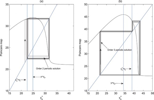
Theorem 4.5

Let $y_{min}^{+}=min\{y^{+}:\varphi (y^{+})=y_P\}$. If $\varphi \left(y_P\right)>y_P$ and ${\varphi }^2\left(y_P\right)<y_{min}^{+}$, then system (2(2) $\left\{\begin{array}{l}\left.\begin{array}{l}\frac{\mathrm{d}x\left(t\right)}{\mathrm{d}t}=rx\left(t\right)\left(1-\frac{x\left(t\right)}{K}\right)-\frac{ax\left(t\right)y\left(t\right)}{1+wx\left(t\right)}\\ \frac{\mathrm{d}y\left(t\right)}{\mathrm{d}t}=\frac{cx\left(t\right)y\left(t\right)}{1+wx\left(t\right)}-\mathrm{d}y\left(t\right)\end{array}\right\}x\left(t\right)<ET,\\ \left.\begin{array}{l}x\left(t^{+}\right)=S_1\left(D\right)x\left(t\right)\\ y\left(t^{+}\right)=S_2\left(D\right)y\left(t\right)+\tau \end{array}\right\}x\left(t\right)=ET,\end{array}\right.$(2) ) exists an order-3 periodic solution.

Proof.

If $\varphi \left(y_P\right)>y_P$, then the results of Theorem 3.1 and Theorem 4.4 reveal that the Poincaré map exists a unique fixed point $y_f$ on $(y_P,\varphi (y_P\left)\right)$. For the existence of an order-3 periodic solution, we only need to find a fixed point $\overline{y}\in [0,+\mathrm{\infty })$ that satisfies ${\varphi }^3\left(\overline{y}\right)=\overline{y}$ and $\varphi \left(\overline{y}\right)\ne \overline{y}$. Further, the results of Theorem 3.1 indicate that ${\varphi }^3\left(y\right)$ is continuous on $[0,+\mathrm{\infty })$, and from the assumptions the Poincaré map ${\varphi }^3$ satisfies

1. ${\varphi }^3$ is increasing on $[0,y_{min})$ and ${\varphi }^3\left(0\right)={\varphi }^2\left(\tau \right)>0$;

2. ${\varphi }^3\left(y_{min}^{+}\right)={\varphi }^2\left(y_P\right)<y_{min}^{+}$.

In the light of the intermediate value theorem and continuity of ${\varphi }^3$, there must be a positive $\overline{y}\in (0,y_{min}^{+})$ that ensures ${\varphi }^3\left(\overline{y}\right)=\overline{y}$ and $y_{min}^{+}<y_P$, and it is clear that $\overline{y}\ne y_f$ because $y_f\in (y_P,\varphi (y_P\left)\right)$. Therefore, the Poincaré map ${\varphi }^3$ exists a fixed point $\overline{y}\in (0,y_{min}^{+})$, and system (2(2) $\left\{\begin{array}{l}\left.\begin{array}{l}\frac{\mathrm{d}x\left(t\right)}{\mathrm{d}t}=rx\left(t\right)\left(1-\frac{x\left(t\right)}{K}\right)-\frac{ax\left(t\right)y\left(t\right)}{1+wx\left(t\right)}\\ \frac{\mathrm{d}y\left(t\right)}{\mathrm{d}t}=\frac{cx\left(t\right)y\left(t\right)}{1+wx\left(t\right)}-\mathrm{d}y\left(t\right)\end{array}\right\}x\left(t\right)<ET,\\ \left.\begin{array}{l}x\left(t^{+}\right)=S_1\left(D\right)x\left(t\right)\\ y\left(t^{+}\right)=S_2\left(D\right)y\left(t\right)+\tau \end{array}\right\}x\left(t\right)=ET,\end{array}\right.$(2) ) exists an order-3 periodic solution (Figure 2b). This completes the proof.

5. Numerical results and biological conclusions

This part mainly deals with two important aspects. The first relates to sensitivity analysis about some key factors with respect to the applications of control tactics. The second involves the bifurcation analysis not only to support our analytical results but also to address how control measures affect the complex dynamics of system (2(2) $\left\{\begin{array}{l}\left.\begin{array}{l}\frac{\mathrm{d}x\left(t\right)}{\mathrm{d}t}=rx\left(t\right)\left(1-\frac{x\left(t\right)}{K}\right)-\frac{ax\left(t\right)y\left(t\right)}{1+wx\left(t\right)}\\ \frac{\mathrm{d}y\left(t\right)}{\mathrm{d}t}=\frac{cx\left(t\right)y\left(t\right)}{1+wx\left(t\right)}-\mathrm{d}y\left(t\right)\end{array}\right\}x\left(t\right)<ET,\\ \left.\begin{array}{l}x\left(t^{+}\right)=S_1\left(D\right)x\left(t\right)\\ y\left(t^{+}\right)=S_2\left(D\right)y\left(t\right)+\tau \end{array}\right\}x\left(t\right)=ET,\end{array}\right.$(2) ), in addition to the outcomes of the control.

5.1. Sensitivity analyses

From Section 4.1, when the predator population dies out and the pest reaches threshold ET, we obtained the expression of the boundary periodic solution $(x^{\mathrm{T}},0)$, and the expression of insecticide dosage was also obtained. These enable us to discuss how the key elements affect the insecticide dosage D. Fixed the parameters as shown in Figure 3, the results show that we must increase the dose D when threshold ET is increasing, and when ET tends to the carrying capacity K, the trend is even more pronounced (Figure 3a). In fact, when ET tends to K, there is only a very small portion of pest population which exceeds ET that needs to be killed. Further, the dose D is increasing when the period T of chemical control is increasing (Figure 3b). Biologically, when T is increasing, the durations between each chemical control are increasing. It indicates that the pest population is exposed to a very small dose of residual pesticides, which results in the reproduction of pest population with fast speed, thereby the dose is also increased. It is claimed that the dose D sprayed in reality needs to take both threshold ET and the period T seriously into account.

Figure 3. The effects of key parameters on the dose D of chemical control: (a) r=1.5, K=100, T=5 and $k_1=0.5$; (b) r=1.5, K=100, ET=35 and $k_1=0.5$.

The threshold condition (13(13) $R_0\triangleq \frac{d}{rD{k}_2}\ln \frac{{\mathrm{e}}^{-k_{1}D}(K-ET)}{K-{\mathrm{e}}^{-k_{1}D}ET}+\frac{cK}{rD{k}_2{k}_1(1+wK)}\ln \frac{(1+wET)(K-{\mathrm{e}}^{-k_{1}D}ET)}{(K-ET)(1+wET{\mathrm{e}}^{-k_{1}D})}<1.$(13) ) provides a simple criterion whether chemical control alone can stabilize the boundary periodic solution or not, that is to say, $R_0<1$ implies that chemical control with dose D alone can control the pest population below threshold ET and vice versa. Thus how the dosage D and threshold ET affect the threshold condition of $R_0$ has attracted wide interests. To do these, we carry out numerical investigations as shown in Figure 4, $R_0\ge 1$ for a small dose D and $R_0<1$ when D exceeds a certain value, and $R_0$ is very sensitive to the parameter c. It reveals that a large dose D can control the pest population below ET when a single chemical control is applied, and the dose D increases as c increases (Figure 4a). In contrary, for a relative small ET we have $R_0<1$, while $R_0\ge 1$ once ET exceeds a certain value. It indicates that for a fixed c a smaller value of ET is more helpful for pest control. Additionally, the earlier the chemical control is implemented, the more beneficial it is to control pests (Figure 4b). Furthermore, if we set D=2, then $R_0>1$ (Figure 4a), and the boundary periodic solution becomes unstable and it suggests that a single chemical control cannot control pests effectively. In this case, the phenomenon of bursting is observed which implies that the pest population outbreaks intermittently with a long period (Figure 5). Because high frequencies of chemical applications will cause insect resistance to insecticides, biological control such as release of natural enemies is a reasonable and effective way to control pest. These results directly reflect the inevitability of integrated implementation of chemical control and biological control.

Figure 4. The effects of control parameters on the threshold condition $R_0$, we set parameters as r=1.5, K=100, a=0.3, w=0.3, d=0.8, $k_1=0.5$, $k_2=0.2$ and $\tau =0$: (a) ET=35; (b) D=0.5.

Figure 5. Time series of system (2(2) $\left\{\begin{array}{l}\left.\begin{array}{l}\frac{\mathrm{d}x\left(t\right)}{\mathrm{d}t}=rx\left(t\right)\left(1-\frac{x\left(t\right)}{K}\right)-\frac{ax\left(t\right)y\left(t\right)}{1+wx\left(t\right)}\\ \frac{\mathrm{d}y\left(t\right)}{\mathrm{d}t}=\frac{cx\left(t\right)y\left(t\right)}{1+wx\left(t\right)}-\mathrm{d}y\left(t\right)\end{array}\right\}x\left(t\right)<ET,\\ \left.\begin{array}{l}x\left(t^{+}\right)=S_1\left(D\right)x\left(t\right)\\ y\left(t^{+}\right)=S_2\left(D\right)y\left(t\right)+\tau \end{array}\right\}x\left(t\right)=ET,\end{array}\right.$(2) ) when $R_0>1$ with parameters fixed as r=1.6, K=100, a=0.3, w=0.3, c=0.5, d=0.8, $k_1=0.5$, $k_2=0.2$, ET=35, $\tau =0$ and D=2.

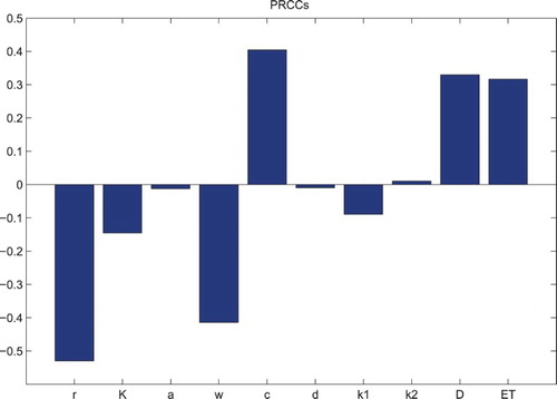
In short, it is found that the dosages in practice play the significant roles in pest control, which relies on all other control parameters. So the question is how to distinguish the parameters from which are beneficial or detrimental for pest control and further to make sure which parameter has greatest effect, moderate effect or little effect on the outcomes of the control? To achieve these, the uncertainty and sensitivity analysis are carried out [2,18,19]. The PRCCs for various input parameters against the condition of $R_0$ with the Latin hypercube sampling (LHS) method of 3000 samples are evaluated, and we use a uniform distribution function to address the significance of all parameters with wide ranges (Figure 6). The results reveal that parameters c, $k_2$, D and ET have positive effects on $R_0$, while parameters r, K, a, w, d and $k_1$ have negative effects on $R_0$. Furthermore, the changes of parameter values of r, w, c, D and ET make great contributions to $R_0$, and parameters K, a, d, $k_1$ and $k_2$ have moderate or little effects on $R_0$. The results indicate how variations of key parameter values affect the successful impulsive control strategies, and it suggests that the dose D and the threshold ET should be chosen carefully not only to control pest population but also to avoid insect resistance.

Figure 6. PRCC results for $R_0$ with baseline parameters fixed as r=1.5, K=100, a=0.3, w=0.3, c=0.225, d=0.8, $k_1=0.5$, $k_2=0.5$, ET=30, $\tau =0$ and D=1.

5.2. Bifurcation analysis

It follows from Theorem 4.5 that there exists an order-3 periodic solution of system (2(2) $\left\{\begin{array}{l}\left.\begin{array}{l}\frac{\mathrm{d}x\left(t\right)}{\mathrm{d}t}=rx\left(t\right)\left(1-\frac{x\left(t\right)}{K}\right)-\frac{ax\left(t\right)y\left(t\right)}{1+wx\left(t\right)}\\ \frac{\mathrm{d}y\left(t\right)}{\mathrm{d}t}=\frac{cx\left(t\right)y\left(t\right)}{1+wx\left(t\right)}-\mathrm{d}y\left(t\right)\end{array}\right\}x\left(t\right)<ET,\\ \left.\begin{array}{l}x\left(t^{+}\right)=S_1\left(D\right)x\left(t\right)\\ y\left(t^{+}\right)=S_2\left(D\right)y\left(t\right)+\tau \end{array}\right\}x\left(t\right)=ET,\end{array}\right.$(2) ) under certain conditions, which means that system (2(2) $\left\{\begin{array}{l}\left.\begin{array}{l}\frac{\mathrm{d}x\left(t\right)}{\mathrm{d}t}=rx\left(t\right)\left(1-\frac{x\left(t\right)}{K}\right)-\frac{ax\left(t\right)y\left(t\right)}{1+wx\left(t\right)}\\ \frac{\mathrm{d}y\left(t\right)}{\mathrm{d}t}=\frac{cx\left(t\right)y\left(t\right)}{1+wx\left(t\right)}-\mathrm{d}y\left(t\right)\end{array}\right\}x\left(t\right)<ET,\\ \left.\begin{array}{l}x\left(t^{+}\right)=S_1\left(D\right)x\left(t\right)\\ y\left(t^{+}\right)=S_2\left(D\right)y\left(t\right)+\tau \end{array}\right\}x\left(t\right)=ET,\end{array}\right.$(2) ) exists periodic solutions with any period [5,11]. We will resort to a one-dimensional bifurcation analysis not only to gain preliminary insight into the possible dynamics of system (2(2) $\left\{\begin{array}{l}\left.\begin{array}{l}\frac{\mathrm{d}x\left(t\right)}{\mathrm{d}t}=rx\left(t\right)\left(1-\frac{x\left(t\right)}{K}\right)-\frac{ax\left(t\right)y\left(t\right)}{1+wx\left(t\right)}\\ \frac{\mathrm{d}y\left(t\right)}{\mathrm{d}t}=\frac{cx\left(t\right)y\left(t\right)}{1+wx\left(t\right)}-\mathrm{d}y\left(t\right)\end{array}\right\}x\left(t\right)<ET,\\ \left.\begin{array}{l}x\left(t^{+}\right)=S_1\left(D\right)x\left(t\right)\\ y\left(t^{+}\right)=S_2\left(D\right)y\left(t\right)+\tau \end{array}\right\}x\left(t\right)=ET,\end{array}\right.$(2) ) but also to verify the theoretical results. As discussed above, the key parameters representing the intensity of control play a critical role in pest control. Thus the dosage D and the release amount of τ are chosen as the bifurcation parameters and we fixed all others as shown in Figure 7. The results show that system (2(2) $\left\{\begin{array}{l}\left.\begin{array}{l}\frac{\mathrm{d}x\left(t\right)}{\mathrm{d}t}=rx\left(t\right)\left(1-\frac{x\left(t\right)}{K}\right)-\frac{ax\left(t\right)y\left(t\right)}{1+wx\left(t\right)}\\ \frac{\mathrm{d}y\left(t\right)}{\mathrm{d}t}=\frac{cx\left(t\right)y\left(t\right)}{1+wx\left(t\right)}-\mathrm{d}y\left(t\right)\end{array}\right\}x\left(t\right)<ET,\\ \left.\begin{array}{l}x\left(t^{+}\right)=S_1\left(D\right)x\left(t\right)\\ y\left(t^{+}\right)=S_2\left(D\right)y\left(t\right)+\tau \end{array}\right\}x\left(t\right)=ET,\end{array}\right.$(2) ) indeed exists periodic solutions with any period as D increases. When D>0, there is an order-3 periodic solution of system (2(2) $\left\{\begin{array}{l}\left.\begin{array}{l}\frac{\mathrm{d}x\left(t\right)}{\mathrm{d}t}=rx\left(t\right)\left(1-\frac{x\left(t\right)}{K}\right)-\frac{ax\left(t\right)y\left(t\right)}{1+wx\left(t\right)}\\ \frac{\mathrm{d}y\left(t\right)}{\mathrm{d}t}=\frac{cx\left(t\right)y\left(t\right)}{1+wx\left(t\right)}-\mathrm{d}y\left(t\right)\end{array}\right\}x\left(t\right)<ET,\\ \left.\begin{array}{l}x\left(t^{+}\right)=S_1\left(D\right)x\left(t\right)\\ y\left(t^{+}\right)=S_2\left(D\right)y\left(t\right)+\tau \end{array}\right\}x\left(t\right)=ET,\end{array}\right.$(2) ) and then system (2(2) $\left\{\begin{array}{l}\left.\begin{array}{l}\frac{\mathrm{d}x\left(t\right)}{\mathrm{d}t}=rx\left(t\right)\left(1-\frac{x\left(t\right)}{K}\right)-\frac{ax\left(t\right)y\left(t\right)}{1+wx\left(t\right)}\\ \frac{\mathrm{d}y\left(t\right)}{\mathrm{d}t}=\frac{cx\left(t\right)y\left(t\right)}{1+wx\left(t\right)}-\mathrm{d}y\left(t\right)\end{array}\right\}x\left(t\right)<ET,\\ \left.\begin{array}{l}x\left(t^{+}\right)=S_1\left(D\right)x\left(t\right)\\ y\left(t^{+}\right)=S_2\left(D\right)y\left(t\right)+\tau \end{array}\right\}x\left(t\right)=ET,\end{array}\right.$(2) ) has a series of chaotic windows, periodic windows and crisis. At last, period-halving bifurcations from chaos leading system (2(2) $\left\{\begin{array}{l}\left.\begin{array}{l}\frac{\mathrm{d}x\left(t\right)}{\mathrm{d}t}=rx\left(t\right)\left(1-\frac{x\left(t\right)}{K}\right)-\frac{ax\left(t\right)y\left(t\right)}{1+wx\left(t\right)}\\ \frac{\mathrm{d}y\left(t\right)}{\mathrm{d}t}=\frac{cx\left(t\right)y\left(t\right)}{1+wx\left(t\right)}-\mathrm{d}y\left(t\right)\end{array}\right\}x\left(t\right)<ET,\\ \left.\begin{array}{l}x\left(t^{+}\right)=S_1\left(D\right)x\left(t\right)\\ y\left(t^{+}\right)=S_2\left(D\right)y\left(t\right)+\tau \end{array}\right\}x\left(t\right)=ET,\end{array}\right.$(2) ) to an order-1 periodic solution (Figure 7a,b). Meanwhile, the outbreak periods of pest populations, which represent the frequency when pest reaches threshold ET, are also drawn with respect to D. Moreover, it is also shown that the release of natural enemies also has great impacts on the complex dynamics of system (2(2) $\left\{\begin{array}{l}\left.\begin{array}{l}\frac{\mathrm{d}x\left(t\right)}{\mathrm{d}t}=rx\left(t\right)\left(1-\frac{x\left(t\right)}{K}\right)-\frac{ax\left(t\right)y\left(t\right)}{1+wx\left(t\right)}\\ \frac{\mathrm{d}y\left(t\right)}{\mathrm{d}t}=\frac{cx\left(t\right)y\left(t\right)}{1+wx\left(t\right)}-\mathrm{d}y\left(t\right)\end{array}\right\}x\left(t\right)<ET,\\ \left.\begin{array}{l}x\left(t^{+}\right)=S_1\left(D\right)x\left(t\right)\\ y\left(t^{+}\right)=S_2\left(D\right)y\left(t\right)+\tau \end{array}\right\}x\left(t\right)=ET,\end{array}\right.$(2) ) (Figure 7c,d). In particular, period-doubling bifurcations from order-1 periodic solution leading system (2(2) $\left\{\begin{array}{l}\left.\begin{array}{l}\frac{\mathrm{d}x\left(t\right)}{\mathrm{d}t}=rx\left(t\right)\left(1-\frac{x\left(t\right)}{K}\right)-\frac{ax\left(t\right)y\left(t\right)}{1+wx\left(t\right)}\\ \frac{\mathrm{d}y\left(t\right)}{\mathrm{d}t}=\frac{cx\left(t\right)y\left(t\right)}{1+wx\left(t\right)}-\mathrm{d}y\left(t\right)\end{array}\right\}x\left(t\right)<ET,\\ \left.\begin{array}{l}x\left(t^{+}\right)=S_1\left(D\right)x\left(t\right)\\ y\left(t^{+}\right)=S_2\left(D\right)y\left(t\right)+\tau \end{array}\right\}x\left(t\right)=ET,\end{array}\right.$(2) ) to chaos and period-halving bifurcations leading system (2(2) $\left\{\begin{array}{l}\left.\begin{array}{l}\frac{\mathrm{d}x\left(t\right)}{\mathrm{d}t}=rx\left(t\right)\left(1-\frac{x\left(t\right)}{K}\right)-\frac{ax\left(t\right)y\left(t\right)}{1+wx\left(t\right)}\\ \frac{\mathrm{d}y\left(t\right)}{\mathrm{d}t}=\frac{cx\left(t\right)y\left(t\right)}{1+wx\left(t\right)}-\mathrm{d}y\left(t\right)\end{array}\right\}x\left(t\right)<ET,\\ \left.\begin{array}{l}x\left(t^{+}\right)=S_1\left(D\right)x\left(t\right)\\ y\left(t^{+}\right)=S_2\left(D\right)y\left(t\right)+\tau \end{array}\right\}x\left(t\right)=ET,\end{array}\right.$(2) ) to an order-1 periodic solution, and the effects of dose D on the frequencies of outbreaks of pest population are also indicated.

Figure 7. Bifurcation diagrams with respect to D and τ when $(K,0)$ is globally stable with parameters fixed as r=1.5, K=100, a=0.3, w=0.3, c=0.225, d=0.8, $k_1=0.5$, ET=35: (a) $\tau =21$ and $k_2=0.3$; (b) D=0.5 and $k_2=0.4$.

It is emphasized that system (2(2) $\left\{\begin{array}{l}\left.\begin{array}{l}\frac{\mathrm{d}x\left(t\right)}{\mathrm{d}t}=rx\left(t\right)\left(1-\frac{x\left(t\right)}{K}\right)-\frac{ax\left(t\right)y\left(t\right)}{1+wx\left(t\right)}\\ \frac{\mathrm{d}y\left(t\right)}{\mathrm{d}t}=\frac{cx\left(t\right)y\left(t\right)}{1+wx\left(t\right)}-\mathrm{d}y\left(t\right)\end{array}\right\}x\left(t\right)<ET,\\ \left.\begin{array}{l}x\left(t^{+}\right)=S_1\left(D\right)x\left(t\right)\\ y\left(t^{+}\right)=S_2\left(D\right)y\left(t\right)+\tau \end{array}\right\}x\left(t\right)=ET,\end{array}\right.$(2) ) also exhibits very rich and complex dynamics when there is an interior equilibrium $E^{\ast }$. For example, assume that the unique $E^{\ast }$ is unstable, we fix all parameters as shown in Figure 8 and then choose the control parameters D and τ as bifurcation parameters. It is shown that model (2(2) $\left\{\begin{array}{l}\left.\begin{array}{l}\frac{\mathrm{d}x\left(t\right)}{\mathrm{d}t}=rx\left(t\right)\left(1-\frac{x\left(t\right)}{K}\right)-\frac{ax\left(t\right)y\left(t\right)}{1+wx\left(t\right)}\\ \frac{\mathrm{d}y\left(t\right)}{\mathrm{d}t}=\frac{cx\left(t\right)y\left(t\right)}{1+wx\left(t\right)}-\mathrm{d}y\left(t\right)\end{array}\right\}x\left(t\right)<ET,\\ \left.\begin{array}{l}x\left(t^{+}\right)=S_1\left(D\right)x\left(t\right)\\ y\left(t^{+}\right)=S_2\left(D\right)y\left(t\right)+\tau \end{array}\right\}x\left(t\right)=ET,\end{array}\right.$(2) ) exhibits very complex dynamics including period-doubling bifurcations, period-halving bifurcations, period-decreasing bifurcations, chaotic windows, periodic windows and crisis (Figure 8). All these results suggest that the control measures not only play a decisive role in the growth and outbreak of pests but also have great impacts on the coexistence of the pests and natural enemies.

Figure 8. Bifurcation diagrams with respect to D and τ when system (2(2) $\left\{\begin{array}{l}\left.\begin{array}{l}\frac{\mathrm{d}x\left(t\right)}{\mathrm{d}t}=rx\left(t\right)\left(1-\frac{x\left(t\right)}{K}\right)-\frac{ax\left(t\right)y\left(t\right)}{1+wx\left(t\right)}\\ \frac{\mathrm{d}y\left(t\right)}{\mathrm{d}t}=\frac{cx\left(t\right)y\left(t\right)}{1+wx\left(t\right)}-\mathrm{d}y\left(t\right)\end{array}\right\}x\left(t\right)<ET,\\ \left.\begin{array}{l}x\left(t^{+}\right)=S_1\left(D\right)x\left(t\right)\\ y\left(t^{+}\right)=S_2\left(D\right)y\left(t\right)+\tau \end{array}\right\}x\left(t\right)=ET,\end{array}\right.$(2) ) exists a unique interior equilibrium $E^{\ast }(x^{\ast },y^{\ast })$: (a) $\tau =7$; (b) D=0.5. All other parameters are fixed as r=1, K=50, a=0.19, w=0.19, c=0.0855, d=0.36, $k_1=0.5$, $k_2=0.4$ and ET=25.

5.3. Comparisons with pulsed model (2) at fixed moments

In reality, the control strategies are often applied with open-loop or closed-loop technics, while open-loop technic is related to control applied at fixed moments and closed-loop technic corresponds to control applied according to the number of pests (i.e. state-dependent feedback control). Fixed all parameters as shown in Figure 9, Figure 9(a) and 9(b) are time series of x and y of model (2(2) $\left\{\begin{array}{l}\left.\begin{array}{l}\frac{\mathrm{d}x\left(t\right)}{\mathrm{d}t}=rx\left(t\right)\left(1-\frac{x\left(t\right)}{K}\right)-\frac{ax\left(t\right)y\left(t\right)}{1+wx\left(t\right)}\\ \frac{\mathrm{d}y\left(t\right)}{\mathrm{d}t}=\frac{cx\left(t\right)y\left(t\right)}{1+wx\left(t\right)}-\mathrm{d}y\left(t\right)\end{array}\right\}x\left(t\right)<ET,\\ \left.\begin{array}{l}x\left(t^{+}\right)=S_1\left(D\right)x\left(t\right)\\ y\left(t^{+}\right)=S_2\left(D\right)y\left(t\right)+\tau \end{array}\right\}x\left(t\right)=ET,\end{array}\right.$(2) ) with period 6.8485, Figures 9(c) and 9(d) are time series of x and y of model (2(2) $\left\{\begin{array}{l}\left.\begin{array}{l}\frac{\mathrm{d}x\left(t\right)}{\mathrm{d}t}=rx\left(t\right)\left(1-\frac{x\left(t\right)}{K}\right)-\frac{ax\left(t\right)y\left(t\right)}{1+wx\left(t\right)}\\ \frac{\mathrm{d}y\left(t\right)}{\mathrm{d}t}=\frac{cx\left(t\right)y\left(t\right)}{1+wx\left(t\right)}-\mathrm{d}y\left(t\right)\end{array}\right\}x\left(t\right)<ET,\\ \left.\begin{array}{l}x\left(t^{+}\right)=S_1\left(D\right)x\left(t\right)\\ y\left(t^{+}\right)=S_2\left(D\right)y\left(t\right)+\tau \end{array}\right\}x\left(t\right)=ET,\end{array}\right.$(2) ) with control applied at fixed moment T=6.8485. The results reveal that model (2(2) $\left\{\begin{array}{l}\left.\begin{array}{l}\frac{\mathrm{d}x\left(t\right)}{\mathrm{d}t}=rx\left(t\right)\left(1-\frac{x\left(t\right)}{K}\right)-\frac{ax\left(t\right)y\left(t\right)}{1+wx\left(t\right)}\\ \frac{\mathrm{d}y\left(t\right)}{\mathrm{d}t}=\frac{cx\left(t\right)y\left(t\right)}{1+wx\left(t\right)}-\mathrm{d}y\left(t\right)\end{array}\right\}x\left(t\right)<ET,\\ \left.\begin{array}{l}x\left(t^{+}\right)=S_1\left(D\right)x\left(t\right)\\ y\left(t^{+}\right)=S_2\left(D\right)y\left(t\right)+\tau \end{array}\right\}x\left(t\right)=ET,\end{array}\right.$(2) ) with state-dependent feedback control can control the pest below ET=35 (Figure 9a,b), but the number of pests is far beyond ET and near the carrying capacity K=100 when control strategies are applied at fixed moments (Figure 9c,d). In this case, to control the pest below the threshold, there are several feasible measures including decreasing period T (Figure 10a); increasing dose D (Figure 10b); decreasing period T and increasing dose D (Figure 10c); increasing both dose D and τ (Figure 10d). However, it is found that after a certain time only increasing the dose D cannot control the pest efficiently because of pest resistance, while increasing release amount τ, or decreasing period T or their combinations not only can control the pest within normal range, but also may decrease pest resistance, which confirms the superiority of biological control.

Figure 9. Time series of system (2(2) $\left\{\begin{array}{l}\left.\begin{array}{l}\frac{\mathrm{d}x\left(t\right)}{\mathrm{d}t}=rx\left(t\right)\left(1-\frac{x\left(t\right)}{K}\right)-\frac{ax\left(t\right)y\left(t\right)}{1+wx\left(t\right)}\\ \frac{\mathrm{d}y\left(t\right)}{\mathrm{d}t}=\frac{cx\left(t\right)y\left(t\right)}{1+wx\left(t\right)}-\mathrm{d}y\left(t\right)\end{array}\right\}x\left(t\right)<ET,\\ \left.\begin{array}{l}x\left(t^{+}\right)=S_1\left(D\right)x\left(t\right)\\ y\left(t^{+}\right)=S_2\left(D\right)y\left(t\right)+\tau \end{array}\right\}x\left(t\right)=ET,\end{array}\right.$(2) ) with different control strategies. (a and b) Control strategies are applied when x reaches ET; (c and d) control strategies are applied with fixed period. All other parameters are fixed as r=1.5, K=100, a=0.3, w=0.3, c=0.225, d=0.8, $k_1=1$, $k_2=0.4$, D=8, $\tau =5$ and ET=35.

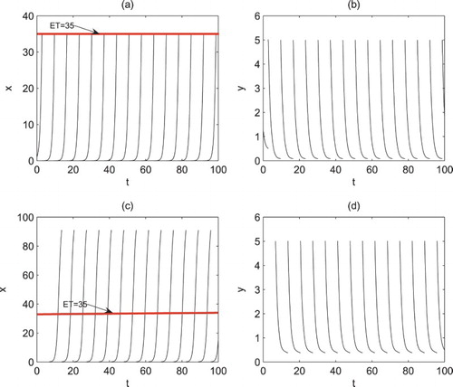
Figure 10. Time series of system (2(2) $\left\{\begin{array}{l}\left.\begin{array}{l}\frac{\mathrm{d}x\left(t\right)}{\mathrm{d}t}=rx\left(t\right)\left(1-\frac{x\left(t\right)}{K}\right)-\frac{ax\left(t\right)y\left(t\right)}{1+wx\left(t\right)}\\ \frac{\mathrm{d}y\left(t\right)}{\mathrm{d}t}=\frac{cx\left(t\right)y\left(t\right)}{1+wx\left(t\right)}-\mathrm{d}y\left(t\right)\end{array}\right\}x\left(t\right)<ET,\\ \left.\begin{array}{l}x\left(t^{+}\right)=S_1\left(D\right)x\left(t\right)\\ y\left(t^{+}\right)=S_2\left(D\right)y\left(t\right)+\tau \end{array}\right\}x\left(t\right)=ET,\end{array}\right.$(2) ) with control strategies applied at fixed periods. (a) T=4.8, D=8 and $\tau =5$; (b) T=6.8458, D=20 and $\tau =5$; (c) T=5, D=15 and $\tau =5$; (d) T=6.8485, D=15 and $\tau =13$. All other parameters are fixed as r=1.5, K=100, a=0.3, w=0.3, c=0.225, d=0.8, $k_1=1$, $k_2=0.4$ and ET=35.

6. Conclusion

Since many problems of human interventions originated from real world need to be mathematically modelled and solved, impulsive semi-dynamical systems, which are described by impulsive differential equations, are often being proposed to model control strategies of closed-loop type, rather than fixed time pulsed model which are used to solve problems of open-loop techniques [17,36,37]. For predator–prey systems with closed-loop control (or state-dependent feedback control), many factors of human actions were investigated including culling, resource limitation, insect resistance, biological and chemical control, media report and so on [16,23,28–30,34,38]. For simplicity, the killing rates or reductions resulting from these elements are usually considered as constants. In order to study the mechanisms of control strategies more profoundly, we proposed a Holling II predator–prey model with insecticide dose as pulsed control. We not only show the global dynamics of system (2(2) $\left\{\begin{array}{l}\left.\begin{array}{l}\frac{\mathrm{d}x\left(t\right)}{\mathrm{d}t}=rx\left(t\right)\left(1-\frac{x\left(t\right)}{K}\right)-\frac{ax\left(t\right)y\left(t\right)}{1+wx\left(t\right)}\\ \frac{\mathrm{d}y\left(t\right)}{\mathrm{d}t}=\frac{cx\left(t\right)y\left(t\right)}{1+wx\left(t\right)}-\mathrm{d}y\left(t\right)\end{array}\right\}x\left(t\right)<ET,\\ \left.\begin{array}{l}x\left(t^{+}\right)=S_1\left(D\right)x\left(t\right)\\ y\left(t^{+}\right)=S_2\left(D\right)y\left(t\right)+\tau \end{array}\right\}x\left(t\right)=ET,\end{array}\right.$(2) ) but also address how variations of doses affect the dynamics, in addition to the outcomes of successful pest control.

First of all, we construct a Poincaré map in the definition domain and then discuss its main properties including monotonicity, differentiability, concavity and existence of fixed points. Subsequently, the expressions of the boundary periodic solution with period T and the exact insecticide dose D are obtained, and then we show this periodic solution is stable under certain condition. The result indicates that a single chemical control can maintain the prey population below threshold ET and may stabilize the pests along this boundary periodic solution. When biological control (i.e. $\tau >0$) is introduced, we investigate the existence and stability of order-$k(k\ge 1)$ periodic solutions, which reveals that the pest and natural enemy populations can not only coexist below ET but also stabilize along order-k periodic solutions.

In order to address biological implications with respect to the key control parameters, we carry out a series of numerical simulations. It is quite evident that the dose D is decreasing when threshold ET is increasing, and the dose D is increasing as the chemical control period T is increasing. Thereby, the insecticide dose D should be sprayed incorporating both threshold ET and period T. Furthermore, threshold condition $R_0$ provides a basic criterion when do we need biological control. For a fixed c, it is found that $R_0$ first increases with $R_0\ge 1$ and then decreases with $R_0<1$ when dose D increases. So a single chemical control with large dose can stabilize the prey population below threshold ET. Meanwhile, $R_0$ first increases with $R_0<1$ and then exceeds 1 as threshold ET increases when we fix c. Thus spraying insecticide earlier is more conducive to pest control. In addition, it is observed that the pest population outbreaks intermittently with high frequencies when $R_0\ge 1$, which increases risk of insect resistance. In this case, biological control such as releasing of natural enemies is initiated to overcome this problem.

Meanwhile, PRCC results demonstrate that control parameters of dose D and threshold ET make great positive contributions to $R_0$. Indeed, biological control together with chemical control not only avoids side effects resulting from a single chemical control but also provides a better way to control pests. Moreover, one-dimensional bifurcations confirm that system (2(2) $\left\{\begin{array}{l}\left.\begin{array}{l}\frac{\mathrm{d}x\left(t\right)}{\mathrm{d}t}=rx\left(t\right)\left(1-\frac{x\left(t\right)}{K}\right)-\frac{ax\left(t\right)y\left(t\right)}{1+wx\left(t\right)}\\ \frac{\mathrm{d}y\left(t\right)}{\mathrm{d}t}=\frac{cx\left(t\right)y\left(t\right)}{1+wx\left(t\right)}-\mathrm{d}y\left(t\right)\end{array}\right\}x\left(t\right)<ET,\\ \left.\begin{array}{l}x\left(t^{+}\right)=S_1\left(D\right)x\left(t\right)\\ y\left(t^{+}\right)=S_2\left(D\right)y\left(t\right)+\tau \end{array}\right\}x\left(t\right)=ET,\end{array}\right.$(2) ) exists periodic solutions of any period. Finally, system (2(2) $\left\{\begin{array}{l}\left.\begin{array}{l}\frac{\mathrm{d}x\left(t\right)}{\mathrm{d}t}=rx\left(t\right)\left(1-\frac{x\left(t\right)}{K}\right)-\frac{ax\left(t\right)y\left(t\right)}{1+wx\left(t\right)}\\ \frac{\mathrm{d}y\left(t\right)}{\mathrm{d}t}=\frac{cx\left(t\right)y\left(t\right)}{1+wx\left(t\right)}-\mathrm{d}y\left(t\right)\end{array}\right\}x\left(t\right)<ET,\\ \left.\begin{array}{l}x\left(t^{+}\right)=S_1\left(D\right)x\left(t\right)\\ y\left(t^{+}\right)=S_2\left(D\right)y\left(t\right)+\tau \end{array}\right\}x\left(t\right)=ET,\end{array}\right.$(2) ) with closed-loop technics can control pest population below a given threshold. However, under same conditions, system (2(2) $\left\{\begin{array}{l}\left.\begin{array}{l}\frac{\mathrm{d}x\left(t\right)}{\mathrm{d}t}=rx\left(t\right)\left(1-\frac{x\left(t\right)}{K}\right)-\frac{ax\left(t\right)y\left(t\right)}{1+wx\left(t\right)}\\ \frac{\mathrm{d}y\left(t\right)}{\mathrm{d}t}=\frac{cx\left(t\right)y\left(t\right)}{1+wx\left(t\right)}-\mathrm{d}y\left(t\right)\end{array}\right\}x\left(t\right)<ET,\\ \left.\begin{array}{l}x\left(t^{+}\right)=S_1\left(D\right)x\left(t\right)\\ y\left(t^{+}\right)=S_2\left(D\right)y\left(t\right)+\tau \end{array}\right\}x\left(t\right)=ET,\end{array}\right.$(2) ) with open-loop technics cannot achieve the purpose of successful pest control, and the feasible measures consist of decreasing period T, increasing dose D, decreasing period T and increasing dose D, in addition to increasing both dose D and τ. Precisely, if a single chemical control is applied after a certain time, then only increasing dose D do not work because of insect resistance. Thus increasing release amount τ plays a decisive role in pest control.

Compared to previous studies with state-dependent feedback control, we summed up some of the highlights of this study: (1) the killing rates or reductions of chemical control are always assumed to be constants. In fact, the killing rates are dosage dependent which have been involved into our model (2(2) $\left\{\begin{array}{l}\left.\begin{array}{l}\frac{\mathrm{d}x\left(t\right)}{\mathrm{d}t}=rx\left(t\right)\left(1-\frac{x\left(t\right)}{K}\right)-\frac{ax\left(t\right)y\left(t\right)}{1+wx\left(t\right)}\\ \frac{\mathrm{d}y\left(t\right)}{\mathrm{d}t}=\frac{cx\left(t\right)y\left(t\right)}{1+wx\left(t\right)}-\mathrm{d}y\left(t\right)\end{array}\right\}x\left(t\right)<ET,\\ \left.\begin{array}{l}x\left(t^{+}\right)=S_1\left(D\right)x\left(t\right)\\ y\left(t^{+}\right)=S_2\left(D\right)y\left(t\right)+\tau \end{array}\right\}x\left(t\right)=ET,\end{array}\right.$(2) ); (2) the existence of periodic solutions is realized by proving existence of fixed points of Poincaré map concerning its main properties; (3) the effects of insecticide dose on the outcomes of a single chemical control or combinations of chemical control and biological control are investigated; (4) bifurcation diagrams show that system (2(2) $\left\{\begin{array}{l}\left.\begin{array}{l}\frac{\mathrm{d}x\left(t\right)}{\mathrm{d}t}=rx\left(t\right)\left(1-\frac{x\left(t\right)}{K}\right)-\frac{ax\left(t\right)y\left(t\right)}{1+wx\left(t\right)}\\ \frac{\mathrm{d}y\left(t\right)}{\mathrm{d}t}=\frac{cx\left(t\right)y\left(t\right)}{1+wx\left(t\right)}-\mathrm{d}y\left(t\right)\end{array}\right\}x\left(t\right)<ET,\\ \left.\begin{array}{l}x\left(t^{+}\right)=S_1\left(D\right)x\left(t\right)\\ y\left(t^{+}\right)=S_2\left(D\right)y\left(t\right)+\tau \end{array}\right\}x\left(t\right)=ET,\end{array}\right.$(2) ) exists very complex dynamics when dose D was chosen as a bifurcation parameter.

For the classical Holling II predator–prey model, we consider the effects of dosage of chemical control on prey and predator as non-linear pulse perturbations, it is assumed that insecticide plays its role in decreasing the pest population once it is sprayed. However, there is a certain time for insecticides from spraying to play the role in killing insect, and this action can be described essentially as hysteresis effect. It is well known that Filippov dynamical systems can provide a natural description for such hysteresis effects [6,32]. It is hoped that such research, planned for the near future and to be reported elsewhere, will be useful for agricultural scientists.

Acknowledgments

The author is very grateful to the anonymous referee for a careful reading, helpful suggestions and valuable comments which led to the improvement of the manuscript.

Disclosure statement

No potential conflict of interest was reported by the authors.

Additional information

Funding

This work was supported by the Chongqing Municipal Education Commission (KJ1600522), Chongqing Science & Technology Commission (cstc2017jcyjAX0131) and by the National Natural Science Foundation of China (NSFC, 11371030, 11301320).

References

- D. Bainov and P. Simeonov, Impulsive Differential Equations: Periodic Solutions and Applications, Longman, Harlow, Vol. 66, 1993.
- S. Blower and H. Dowlatabadi, Sensitivity and uncertainty analysis of complex-models of disease transmission? An HIV model, as an example, Int. Stat. Rev. 62 (1994), pp. 229–243.
- K. Ciesielski, On time reparametrizations and isomorphisms of impulsive dynamical systems, Ann. Polon. Math. 84 (2004), pp. 1–25.
- C.J. Dai, M. Zhao and L.S. Chen, Homoclinic bifurcation in semi-continuous dynamic systems, Int. J. Biomath. 05 (2012), 1250059, 19 pages.
- R. Devaney, An Introduction to Chaotic Dynamical Systems, Addison-Wesley, New York, 1989.
- A.F. Filippov, Differential Equations with Discontinuous Righthand Sides, Kluwer Academic, Dordrecht, 1988.
- M.Z. Huang, J.X. Li, X.Y. Song and H.J. Guo, Modeling impulsive injections of insulin: towards artificial pancreas, SIAM J. Appl. Math. 72 (2012), pp. 1524–1548.
- S.U. Karaagac, Insecticide Resistance, InTech Press, London, 2012.
- S. Kaul, On impulsive semidynamical systems, J. Math. Anal. Appl. 150 (1990), pp. 120–128.
- Y. Kuang and H.I. Freedman, Uniqueness of limit cycles in Gause-type models of predator–prey systems, Math. Biosci. 88 (1988), pp. 67–84.
- T. Li and J. Yorke, Period three implies chaos, Amer. Math. 82 (1975), pp. 985–992.
- J.H. Liang, S.Y. Tang, R.A. Cheke and J.H. Wu, Adaptive release of natural enemies in a pest-natural enemy system with pesticide resistance, Bull. Math. Biol. 75 (2013), pp. 2167–2195.
- X.N. Liu and L.S. Chen, Complex dynamics of Holling type II Lotka–Volterra predator–prey system with impulsive perturbations on the predator, Chaos Solitons Fractals 16 (2003), pp. 311–320.
- B. Liu, Z.D. Teng and L.S. Chen, Analysis of a predator–prey model with Holling II functional response concerning impulsive control strategy, J. Comput. Appl. Math. 193 (2006), pp. 347–362.
- B. Liu, Y. Tian and B.L. Kang, Dynamics on a Holling II predator–prey model with state-dependent impulsive control, Int. J. Biomath. 5 (2012), 18 pages.
- Y. Liu, X. Zhang and T. Zhou, Multiple periodic solutions of a delayed predator–prey model with non-monotonic functional response and stage structure, J. Biol. Dyn. 8(1) (2014), pp. 145–160.
- Y. Lv, R. Yuan and Y. Pei, Two types of predator–prey models with harvesting: non-smooth and non-continuous, J. Comput. Appl. Math. 250 (2013), pp. 122–142.
- S. Marino, I.B. Hogue, C.J. Ray and D.E. Kirschner, A methodology for performing global uncertainty and sensitivity analysis in systems biology, J. Theor. Biol. 254 (2008), pp. 178–196.
- M.D. McKay, R.J. Beckman and W.J. Conover, A comparison of three methods for selecting values of input variables in the analysis of output from a computer code, Technometrics. 21 (1979), pp. 239–245.
- J.C. Panetta, A mathematical model of periodically pulsed chemotherapy: tumor recurrence and metastasis in a competitive environment, Bull. Math. Biol. 58 (1996), pp. 425–447.
- W.J. Qin, S.Y. Tang and R.A. Cheke, The effects of resource limitation on a predator–prey model with control measures as nonlinear pulses, Math. Probl. Eng. 2014 (2014), 14pages.
- P. Simeonov and D. Bainov, Orbital stability of periodic solutions of autonomous systems with impulsive effect, Int. J. Systems Sci. 19 (1988), pp. 2561–2585.
- K.B. Sun, T.H. Zhang and Y. Tian, Theoretical study and control optimization of an integrated pest management predator–prey model with power growth rate, Math. Biosci. 279 (2016), pp. 13–26.
- S.Y. Tang and R.A. Cheke, Models for integrated pest control and their biological implications, Math. Biosci. 215 (2008), pp. 115–125.
- S.Y. Tang, Y.N. Xiao and R.A. Cheke, Multiple attractors of host-parasitoid models with integrated pest management strategies: eradication, persistence and outbreak, Theor. Popul. Biol. 73 (2008), pp. 181–197.
- S.Y. Tang, Y.N. Xiao and R.A. Cheke, Effects of predator and prey dispersal on success or failure of biological control, Bull. Math. Biol. 71 (2009), pp. 2025–2047.
- S.Y. Tang, Y.N. Xiao and R.A. Cheke, Dynamical analysis of plant disease models with cultural control strategies and economic thresholds, Math. Comput. Simulat. 80 (2010), pp. 894–921.
- S.Y. Tang, W.H. Pang, R.A. Cheke and J.H. Wu, Global dynamics of a state-dependent feedback control system, Adv. Differ. Equ. 2015 (2015), pp. 322.
- S.Y. Tang, B. Tang, A.L. Wang and Y.N. Xiao, Holling II predator–prey impulsive semi-dynamic model with complex Poincaré map, Nonlinear Dynam. 81 (2015), pp. 1575–1596.
- S.Y. Tang, Y.N. Xiao and J.H. Wu, Media impact switching surface during an infectious disease outbreak, Sci. Rep. 5 (2015), pp. 672.
- M.B. Thomas, Ecological approaches and the development of truly integrated pest management, Proc. Natl. Acad. Sci. 96 (1999), pp. 5944–5951.
- V.I. Utkin, J. Guldner and J.X. Shi, Sliding Mode Control in Electro-mechanical Systems, 2nd ed., Taylor & Francis Group, Boca Raton, 2009.
- J.C. Van Lenteren and J. Woets, Biological and integrated pest control in greenhouses, Annu. Rev. Entomol. 33 (1988), pp. 239.
- Y.P. Wang, M. Zhao, X.H. Pan and C.J. Dai, Dynamic analysis of a phytoplankton-fish model with biological and artificial control, Discrete Dyn. Nat. Soc. 2014 (2014). doi:doi: 10.1155/2014/914647.
- J. Yang and S.Y. Tang, Holling type II predator–prey model with nonlinear pulse as state-dependent feedback control, J. Comput. Appl. Math. 291 (2016), pp. 225–241.
- J. Yang, S.Y. Tang and Y.S. Tan, Complex dynamics and bifurcation analysis of host-parasitoid models with impulsive control strategy, Chaos Soliton. Fract. 91 (2016), pp. 522–532.
- J. Yang, G.Y. Tang and S.Y. Tang, Modelling the regulatory system of a chemostat model with a threshold window, Math. Comput. Simulat. 132 (2017), pp. 220–235.
- T.Q. Zhang, W.B. Ma, X.Z. Meng and T.H. Zhang, Periodic solution of a prey–predator model with nonlinear state feedback control, Appl. Math. Comput. 266 (2015), pp. 95–107.