
 ?Mathematical formulae have been encoded as MathML and are displayed in this HTML version using MathJax in order to improve their display. Uncheck the box to turn MathJax off. This feature requires Javascript. Click on a formula to zoom.
ABSTRACT
In meta-population models for infectious diseases, the basic reproduction number can be as much as 70% larger in the case of preferential mixing than that in homogeneous mixing [J.W. Glasser, Z. Feng, S.B. Omer, P.J. Smith, and L.E. Rodewald, The effect of heterogeneity in uptake of the measles, mumps, and rubella vaccine on the potential for outbreaks of measles: A modelling study, Lancet ID 16 (2016), pp. 599–605. doi: 10.1016/S1473-3099(16)00004-9]. This suggests that realistic mixing can be an important factor to consider in order for the models to provide a reliable assessment of intervention strategies. The influence of mixing is more significant when the population is highly heterogeneous. In this paper, another quantity, the final epidemic size (
) of an outbreak, is considered to examine the influence of mixing and population heterogeneity. Final size relation is derived for a meta-population model accounting for a general mixing. The results show that
can be influenced by the pattern of mixing in a significant way. Another interesting finding is that, heterogeneity in various sub-population characteristics may have the opposite effect on
and
.
1. Introduction
Epidemiological models can be used to identify key factors affecting disease outbreaks and to evaluate intervention strategies. However, because the model predictions and evaluations can be influenced by assumptions made to simplify the analysis, it is critical to understand how certain simplifying assumptions may affect the model outcomes, particularly if the models are used to inform public health policy-making.
One of the most commonly used assumptions in epidemiological models is the homogeneous, or random, mixing in the whole population, which allows the model to ignore heterogeneity in various sub-population factors including activity (pertinent to disease transmission), susceptibility, preference in contact, group size, etc. Although these simplifying assumptions are reasonable in many cases depending on the questions to be studied, there are cases where these heterogeneous factors cannot be ignored (see e.g. [Citation11–13]).
When epidemic models are used to evaluate strategies for disease control and prevention, the quantities used often include the basic or effective reproduction number ( or
), the final epidemic size (
), and the peak size of an outbreak (
). Andreasen [Citation2] studied the role of heterogeneity in susceptibility and infectiousness on final epidemic size for the case of proportionate mixing and discussed the relationship between
and
. Tildesley and Keeling [Citation19] considered a model with a spatial structure to discuss the issue of using
as a predictor of final epidemic size for the case of foot-and-mouth disease in the UK. Results concerning final epidemic sizes can also be found in other studies including [Citation1,Citation3,Citation4,Citation10,Citation15,Citation16]. None of these studies considered the influence of heterogeneity on the final size or the relationship between
and
in a meta-population with preferential mixing.
In this paper, we consider an epidemic meta-population model that includes a general mixing function (which includes proportionate, preferential, and homogeneous mixing as special cases). We examine how heterogeneity in various sub-population factors may influence ,
, and
, and how preferential mixing may affect the relationship between
and
. Our results show that models that do not account for heterogeneous mixing may produce biased or even incorrect information.
From previous epidemic models with homogeneous mixing, a general understanding is that and
are positively related (see Figure ). We show in this paper that, when preferential mixing is considered in the model with heterogeneity in activity and/or preference, it is possible that
and
are negatively related (see Figures and ). Moreover, when vaccination is considered, the homogeneous coverage may not be the most effective strategy (see Figures and ).
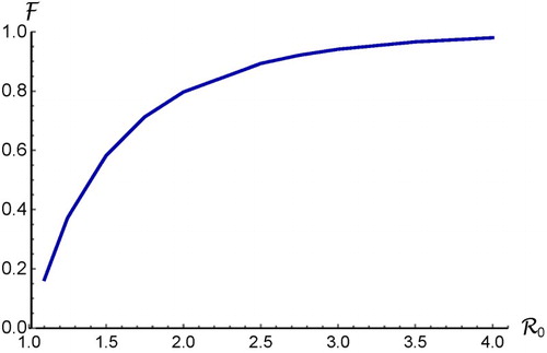
Figure 1. Plot of the final size relation given in (Equation18(18)
(18) ) for the case of a homogeneous population with random mixing. It shows that
is an increasing function of
.
The paper is organized as follows. In Section 2, we present the model with n sub-populations and non-homogeneous mixing. Derivations for the reproduction number and a final epidemic size relation are also included in this section. Section 3 focuses on the investigation of the effects of heterogeneity in various sub-population factors and mixing on the final epidemic size and epidemic peak during an outbreak. Two examples of using the meta-population model to evaluate intervention strategies are also presented in this section. Section 4 includes discussions of the results.
2. The model and final epidemic size
Consider a meta-population with n sub-populations or groups with sizes (
). The population in each group i is divided into three epidemiological classes denoted by
(susceptible),
(infectious), and
(recovered and immune due to infection). Thus,
(
). Because we are concerned with the final epidemic size of a single disease outbreak, births and deaths are ignored. The epidemic model with n sub-groups consists of the following ordinary differential equations:
(1)
(1) with initial conditions:
(2)
(2) In model (Equation1
(1)
(1) ),
is the per capita contact rate (referred to as activity),
is the probability that a susceptible person in group i becomes infected upon contacting an infectious person, γ denotes the per-capita recovery rate. The contacts between sub-groups are described by the mixing matrix
, where
is the proportion of the ith sub-group's contacts that is with members of the jth group, and
is the probability that a randomly encountered member of group j is infectious. As pointed out in Busenberg and Castillo-Chavez [Citation6], a mixing function needs to satisfy the following basic conditions:
(3)
(3) One of the commonly used mixing functions, as originally considered by Nold [Citation17] and later extended by Jacquez et al. [Citation14], is the preferential mixing with the form:
(4)
(4) In the preferential mixing (Equation4
(4)
(4) ),
denotes the fraction of contacts reserved for one's own group (referred to as preferences), and
is the Kronecker delta (1 when i=j and 0 otherwise). The function
describes mixing that is random, i.e. proportional to unreserved contacts,
. All parameters are non-negative.
The isolated basic reproduction number for group i is
(5)
(5) The next generation matrix is
(6)
(6) where
is the mixing matrix. The basic reproduction number for the meta-population is
(7)
(7) when
denotes the dominant eigenvalue of K. In general, we can only compute
numerically when n>2. Two special cases are when the mixing is proportionate (i.e. when
) or isolated (i.e. when
) for all i. In these cases,
is given by either the trace of K or the maximum of
. That is, the analytic expressions are:
(8)
(8) If vaccines are available before the epidemic starts, a certain level of population immunity can be achieved via vaccination. Let
denote the immunity of sub-population i at time t=0 (
). Then the disease dynamics can be modelled by the equations in (Equation1
(1)
(1) ) with modified initial conditions:
(9)
(9) In this case, the isolated effective reproduction number for group i is
, and the next generation matrix is
. The effective reproduction number for the meta-population is
.
If the effect of another type of control or intervention programme is to reduce activities and/or probabilities of infection
, let
denote the isolated effective reproduction number for group i (same formula as for
in (Equation5
(5)
(5) ) but with the new values of
and
), then the effective reproduction number for the meta-population
is given by the dominant eigenvalue of the next generation matrix
, which is the same as K in (Equation6
(6)
(6) ) but with
being replaced by
.
We now use (Equation1(1)
(1) ) with initial condition (Equation2
(2)
(2) ) to derive a relation for the final epidemic size. Note from the
and
equations in (Equation1
(1)
(1) ) that
(10)
(10) Because
and
for all t>0,
is a non-negative decreasing function and hence has a limit as
and
. It follows that
as
(see [Citation5], Section 2.4). Thus,
exists. Using
and
, and from (Equation10
(10)
(10) ) we get
(11)
(11) Dividing the
equation in (Equation1
(1)
(1) ) by
on both sides, we get
(12)
(12) Integration of both sides of (Equation12
(12)
(12) ) from 0 to ∞ yields
(13)
(13) From (Equation11
(11)
(11) ), (Equation13
(13)
(13) ), and
, we obtain
(14)
(14) Let
, then
(15)
(15) Thus, from (Equation14
(14)
(14) ) and (Equation15
(15)
(15) ), we know that
can be determined by a solution of the following set of equations:
(16)
(16) Let
denote the total population size, and let
denote the fraction of infected in group i (over the total N). We define the final epidemic size
by
(17)
(17) In the special case when the population is considered homogeneous with random mixing, i.e. the parameter values for all sub-groups are identical (e.g.
,
,
,
,
are all independent of i and
), the final size relation simplifies to
(18)
(18) where
and
. If we vary
by varying β while keeping a and γ fixed, the final size relation (Equation18
(18)
(18) ) is illustrated in Figure , which shows that
is an increasing function of
.
As shown in Feng et al. [Citation11] and Glasser et al. [Citation13], in meta-population models with preferential mixing, even when β and the mean activity are constant (with all other parameter values fixed),
may vary with the level of heterogeneity in
and preference
. Therefore, the dependence of
on
may not be increasing as exhibited in Figure . In the following sections, we will investigate how population heterogeneity in models with non-random mixing may influence the final size
, the relationship between
and
, and model evaluations of intervention programmes.
3. Effect of heterogeneity on final size and the relationship between  and
and
A general understanding based on epidemic models for a homogeneous population with random mixing is that is an increasing function of
, as shown in Figure . Recall that the increase in
is caused by increasing β. When heterogeneity such as activity (
), preference of contacts (
), and sub-population size (
) are considered in a meta-population model with preferential mixing,
may vary by a significantly magnitude even when
are fixed (see e.g. [Citation13]). In addition, it has been shown in Poghotanyan et al. [Citation18] that, among a large class of mixing matrices
including the preferential mixing in (Equation4
(4)
(4) ),
is bounded below and above by the basic reproduction numbers corresponding to proportionate mixing (
for all i) and isolated mixing (
for all i), respectively, i.e.
(19)
(19) where
It is clear from (Equation19
(19)
(19) ) that we can keep
fixed and change
by varying
and
while keeping the same mean activity and mean population size. Particularly, different
values may also affect how
and
may be influenced by heterogeneity in
or
. Thus, the relationship between
and
may be more complex in meta-population models than the one illustrated in Figure . This will be explored next.
Results in this section are for the case of n=2 groups, but they can be extended to the case of n>2. Although the equations for in (Equation16
(16)
(16) ) cannot be solved analytically, we can explore the dependence of
on other parameters numerically. Rewrite (Equation16
(16)
(16) ) as
(20)
(20) where
(21)
(21) Figure (a) illustrates the final size as an intersection of the curves determined by F=1 and G=1.
Figure 2. (a) The solution of the equations (Equation21
(21)
(21) ) is shown as the intersection of the curves
and
. (b) Cumulative infections during an outbreak in the two groups and the total. The plots are for the case of proportionate mixing (i.e.
) with
, and
.
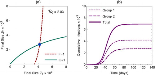
For demonstration purposes, we used the following parameter values in Figure (the time unit is days): ,
(infectious period is 5 days),
with
and
(heterogeneous activity with the mean activity being 10),
(proportionate mixing),
,
(homogeneous sub-population size with
), and
. For these parameter values, the isolated reproduction numbers for sub-populations 1 and 2 are
and
, respectively. The overall effective reproduction number for the meta-population is
. From the equations in (Equation16
(16)
(16) ), we have
and
. These values are also consistent with the cumulative infections in groups 1 and 2 presented in Figure (b) from numerical simulations of system (Equation1
(1)
(1) ) with the initial condition (Equation2
(2)
(2) ).
3.1. Influence of heterogeneity and non-homogeneous mixing
To explore the effect of mixing on model predictions, we consider preferential mixing (Equation4(4)
(4) ) and examine heterogeneity in various characteristics affecting the mixing function including activity
, group size
, and preference
. For demonstration purposes, we fix the same parameter values
,
, and the mean activity
. Values for other parameters may vary depending on applications.
3.1.1. Heterogeneity in activity
Consider first the case of proportionate mixing (). The effect of heterogeneity and variability in activity
on
is illustrated in Figure , which shows the final sizes for three sets of activities
. The
values used in the three rows from top to bottom are (with increasing variability)
The left column shows the values of
determined by equations in (Equation16
(16)
(16) ), as the intersection of F=1 and G=1 (marked by the dot). The right column shows the epidemic curves based on the simulations of the system (Equation1
(1)
(1) ) with initial condition (Equation2
(2)
(2) ). Notice that the number of individuals in the R class represents the cumulative infections at anytime.
Figure 3. Comparison of ,
, and
when activity is homogeneous (top) and heterogeneous with increasing variance (middle and bottom). Mixing is proportional (
). The left column shows the final size (marked by the point of intersection of F=1 and G=1 as the solution of (Equation20
(20)
(20) )). The right column shows the the total sizes of S, I, and R as the solution of model (Equation1
(1)
(1) ) with initial condition (Equation2
(2)
(2) ).
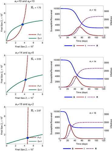
In this case, the basic reproduction numbers are , and 2.87, respectively, while the final sizes are
and 0.599, respectively. We observe the following changes as the variability in activity increases
the time to epidemic peak decreases.
To make it more transparent how variability in affects
,
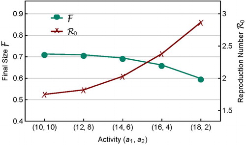
, and their relationship, Figure plots
and
for several sets of activity
that have the same mean. It shows that the homogeneous activity (
) corresponds to the smallest
and largest
, while the heterogeneous activity with the highest variability (
) corresponds to the largest
and smallest
. This provides an example that the final size does not vary with
positively. That is, the usual understanding based on models with homogeneous assumption that
increases with
(see Figure ) may not be true when more realistic mixing functions are incorporated in meta-population models. Such results may have important implications for public health policy-making. For example, when a control programme is aimed at reducing
, it should also check whether or not it may lead to an increased final epidemic size.
Figure 4. Plots of and
for contact rates
and
with the same mean but different variability. When
changes from (10,10) to (18,2),
increases from 1.75 to 2.87 whereas
decreases from 0.713 to 0.599.
3.1.2. Preference level in mixing
The examples in Section 3.1.1 are for proportionate mixing (i.e. ). A more realistic mixing, in general, is when
, representing a preference of contacts with others in the same sub-group. Heterogeneity in factors such as
and
may have an important influence in
and
, as suggested in (Equation19
(19)
(19) ). We now explore the effect of variability in
and the joint effect of
and
on
and
. Consider first the simpler case when
. Figure provides a similar information as in Figure but includes cases of
.
Figure 5. Plots of and
for various preference level
and activity variability in
(with equal mean
), showing that as
or variability in
increases,
decreases while
increases.
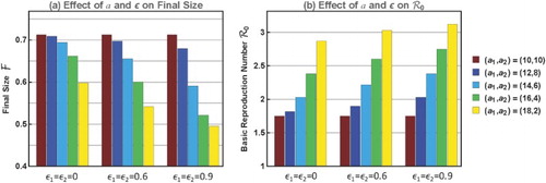
We observe in Figure that (i) for each fixed value,
increases but
decreases with the variability in
, and the changes are more dramatic for higher
; and (ii) for each fixed heterogeneous pair
,
increases and
decreases with
. Because the bar charts in Figure (a,b) are for the same sets of
and
, it shows again that
and
are related negatively when heterogeneity in
and/or
is varied. This illustrates again an opposite relationship between
and
to that shown in Figure .
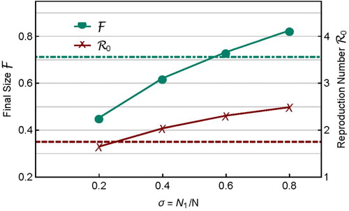
3.1.3. Sub-population size
The influence of heterogeneity in can be examined by fixing all other parameter values. For example, Figure shows the case when
,
,
, and all other parameter values except
are the same as before. The total
is fixed but
varies. It shows that both
and
increase with σ, and thus, in this case,
and
are positively related. The values of
and
for the homogeneous case (
and
) are also shown by the dot-dashed and dashed lines, respectively. Thus, heterogeneity in characteristics including
and
can either increase or decrease
and
.
Figure 6. Changes in and
with the sub-population sizes
(
and
for fixed N). The dot-dashed line and dashed line are values of
and
, respectively, for homogeneous case in which
and
.
3.2. Examples
Because population heterogeneity in factors such as or
may affect the final size and the basic reproduction number in significant ways, we investigate in this section how the model evaluations of intervention strategies may be affected. Two examples are discussed below.
3.2.1. Heterogeneity in vaccine coverage
Consider the model equations in (Equation1(1)
(1) ) with the initial condition in (Equation9
(9)
(9) ). Assume that the vaccine efficacy is 100% so that the vaccination coverage in group i is the same as the immunity
, and the total number of vaccine doses is
. When
with fixed total size
, fixing the total number of vaccine doses is equivalent to fixing the value of
. Thus, we can examine the effect of heterogeneity in vaccine allocation
on
and
for fixed p. Choose parameter values to be the same as before except that
,
,
,
, and
. For these parameter values, the basic reproduction numbers for the two groups are
and
with
. For demonstration purpose, let
. For the homogeneous case (
and
), the final size is
and the effective reproduction number is
, which are labelled in Figure by the dot-dashed and dashed lines, respectively.
Figure 7. Similar to Figure , but this shows the dependence of and
on heterogeneity in sub-population immunity
with
. The dot-dashed line and dashed line are values of
and
, respectively, for the homogeneous case with
and
.
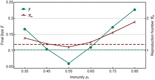
In Figure , and
for several sets of heterogeneous coverage with
are plotted. It is interesting to notice that for
, both
and
are smaller than their corresponding values in the homogeneous case,
and
(shown by the dot-dashed and dashed lines). But for other
values,
and
. This shows that, for a fixed amount of vaccine doses, although the homogeneous coverage
can provide a relatively more effective allocation than many heterogeneous vaccine allocations in reducing
, it may not be the best choice. This result is consistent with those found in Feng et al. [Citation11], in which it is shown that the optimal vaccine allocation can be determined using a gradient approach based on a Lagrange optimization problem. The results in Feng et al. [Citation11] is formulated in terms of minimizing the effective reproduction number.
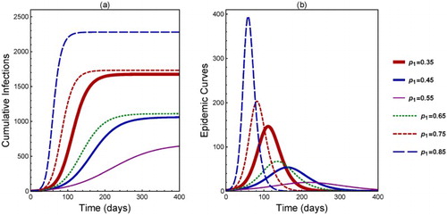
In addition to the final size, the peak size () and time to peak (
) are also sensitive to the heterogeneity in
. This is illustrated in Figure (the
values for different curves are labelled in the legend). All parameter values are the same as in Figure .
We observe in Figure (a) that, as increases from 0.35 to 0.55, the number of cumulative infections decreases (see the solid curves). However, as
continues to increase to 0.65 until 0.85, the number of cumulative infections becomes increasing (the dot-dashed to dashed curves). Similarly in Figure (b),
and
decrease from
to 0.55 (solid curves) but increase from
to 0.85 (dashed curves).
3.2.2. The 2011 acute haemorrhagic conjunctivitis outbreak in China
In this section, we examine how population heterogeneity in various characteristics may affect model evaluations of control and intervention programmes. We demonstrate this by using an example based on the 2011 outbreak of AHC in Changsha, China. Studies on the efficacy of quarantine during this outbreak is presented in [Citation7,Citation8]. By fitting a homogeneous SIR model to the data from a case report for a school population, they obtained an estimate for the transmission coefficient β. Based on this, we adopt as a baseline value for the probability of infection on contact with a baseline value for activity to be a=15. The infectious period for this AHC outbreak in China is about 7–10 days, so we choose
to be 8 days. Under these parameter values, the baseline value for the reproduction number is
. This is much higher than the value of the reproduction number
presented in [Citation9] for the 2003 AHC outbreak in Mexico, where
. The main reason for this difference is in the value of infectious period, which are about 8 and 3 days for the outbreaks in China and Mexico, respectively.
Consider the case when the population is divided into two groups, and individuals in group 1 have a lower risk of being infected due to a reduced contact rate, better health habit (e.g. washing hands to increase protection against infection) or other behavioural changes as suggested by public health officials. Thus, let (baseline value) and
(e.g. a school population) be fixed. Assume that individuals in the low risk group have a reduced activity with
(
), and let
The mixing is assumed to be proportionate. We will examine the changes in
due to interventions aimed at decreasing δ and increasing σ. The simulation results are presented in Figure , which shows the model evaluations for the effect of reducing δ and increasing σ on the final epidemic size
.
Figure 9. Effect of reducing δ (transmission coefficient) and increasing σ (proportion of the low-risk group) on .
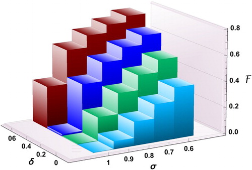
We observe in Figure that increasing σ can be effective in reducing the final size only if δ is sufficiently small. For example, if 60% of individuals are in group 1 () and the reduction factor for the risk of infection is
, the final size is 0.79. The reason for the high percentage of cumulative infections is because of the high value of the basic reproduction number
for group 2. In fact, in the absence of control, almost the entire population will be infected during the outbreak. For the same value of
, even when
, the final size will still be as high as 32%. The only possibility to have the final size below 10% is when
and
. However, as long as
(or
), there will be a significant number of infections.
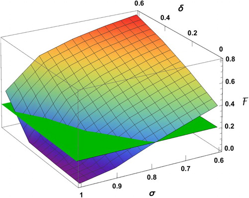
Figure plots the surface of the final size as a function of δ and σ, which is obtained by connecting the values of the bar chart. We can identify the region in the () plane in which the final size is below a certain level. For example, the intersection curve of the
surface with the plane with
determines the proportion σ of individuals in group 1 (for a given δ value), above which the final size is below 20%.
Figure 10. The surface is a plot of the final size versus δ and σ, and the plane corresponds to
. The intersection curve identifies the region for
(where the surface is below the plane) in which the final size is below 20%.
4. Discussion
The results presented in this paper provide another example that incorporation of population heterogeneity and non-homogeneous mixing in epidemic models can generate outcomes that are qualitatively different from that based on models for populations with homogeneous mixing. Particularly, for two of the most important quantities, reproduction number ( or
) and final epidemic size (
), we demonstrated how they may be influenced by population heterogeneity in various characteristics and mixing by comparing the results from a meta-population model with and without heterogeneity and non-homogeneous mixing. The final epidemic size relation and the reproduction number derived from the meta-population model (Equation1
(1)
(1) ) with a general mixing matrix
allows us to conduct various comparisons (see Sections 3.1.1–3.1.3). We also presented two examples to illustrate the effect of heterogeneity and mixing in the model evaluation of intervention strategies (Section 3.2). An interesting result is that, although homogeneous vaccine coverage may produce higher reduction in
than many heterogeneous combinations of coverage, it may not be the most effective option (see Figures and ) if the objective is to maximally reduce
for a given number of vaccine doses.
Another interesting finding of this study is the correlation between and
. In models with homogeneous mixing,
and
are positively related, as shown in Figure . However, this relation may be reversed when heterogeneity is considered in a meta-population model with non-homogeneous mixing, as illustrated in Figures and . Particularly, an increase of variability in activity (
) or preference level (
) can increase
but decrease
. Thus, in this case,
and
are negatively related. The finding that
can be increased by population heterogeneity in various factors is also supported by the fact pointed out by Tilman and Kareiva [Citation20] that
is higher in situations with significant spatial or heterogeneity features.
The final size relation derived in this paper from a meta-population model, which considers n sub-populations, multiple types of heterogeneity, and a general mixing function including preferential mixing, provides a useful evaluation tool for intervention strategies. It also raised the warning issue that, although in many models control measures can be evaluated using the effective reproduction number , it should not be the only quantity to consider, especially if a programme reduces
but increases
.
Acknowledgements
We thank John Glasser for reading the manuscript and providing many constructive suggestions that improved the presentation of this paper. We thank also the Reviewer for helpful comments.
Disclosure statement
No potential conflict of interest was reported by the authors.
Additional information
Funding
References
- R.M. Anderson and R.M. May, Infectious Diseases of Humans: Dynamics and Control, Cambridge University Press, New York, 1991.
- V. Andreasen, The final size of an epidemic and its relation to the basic reproduction number, Bull. Math. Biol. 73 (2011), pp. 2305–2321. doi: 10.1007/s11538-010-9623-3
- J. Arino, F. Brauer, P. van den Driessche, J. Watmough, and J. Wu, A final size relation for epidemic models, Math. Biosci. Eng. 4 (2007), pp. 159–175. doi: 10.3934/mbe.2007.4.159
- F. Brauer, Epidemic models with heterogeneous mixing and treatment, Bull. Math. Biol. 70 (2008), pp. 1869–1885. doi: 10.1007/s11538-008-9326-1
- F. Brauer, C. Castillo-Chavez, and Z. Feng, Mathematical Models in Epidemiology, Springer, 2018, to appear
- S. Busenberg and C. Castillo-Chavez, A general solution of the problem of mixing of subpopulations and its application to risk-and age-structured epidemic models for the spread of AIDS, IMA J. Math. Appl. Med. Biol. 8 (1991), pp. 1–29. doi: 10.1093/imammb/8.1.1
- T. Chen, R. Liu, and Q. Wang, Application of susceptible-infected-recovered model in dealing with an outbreak of acute hemorrhagic conjunctivitis on one school, Chin. J. Epidemiol. 32 (2011), pp. 723–726.
- T. Chen and R. Liu, Study of the efficacy of quarantine during outbreaks of acute hemorrhagic conjunctivitis at schools through the susceptive-infective-quarantine-removal-model, Chin. J. Epidemiol. 34 (2013), pp. 75–79.
- G. Chowell, E. Shim, F. Brauer, P. Diaz-Dueñas, J.M. Hyman, and C. Castillo-Chavez, Modelling the transmission dynamics of acute haemorrhagic conjunctivitis: Application to the 2003 outbreak in Mexico, Stat. Med. 25 (2006), pp. 1840–1857. doi: 10.1002/sim.2352
- Z. Feng, Final and peak epidemic sizes for SEIR models with quarantine and isolation, Math. Biosci. Eng. 4 (2007), pp. 675–686. doi: 10.3934/mbe.2007.4.675
- Z. Feng, A.N. Hill, P.J. Smith, and J.W. Glasser, An elaboration of theory about preventing outbreaks in homogeneous populations to include heterogeneity or preferential mixing, J. Theor. Biol. 386 (2015), pp. 177–187. doi: 10.1016/j.jtbi.2015.09.006
- Z. Feng, A.N. Hill, A.T. Curns, and J.W. Glasser, Evaluating targeted interventions via meta-population models with multi-level mixing, Math. Biosci. 287 (2017), pp. 93–104. doi: 10.1016/j.mbs.2016.09.013
- J.W. Glasser, Z. Feng, S.B. Omer, P.J. Smith, and L.E. Rodewald, The effect of heterogeneity in uptake of the measles, mumps, and rubella vaccine on the potential for outbreaks of measles: A modelling study, Lancet ID 16 (2016), pp. 599–605. doi: 10.1016/S1473-3099(16)00004-9.
- J.A. Jacquez, C.P. Simon, J. Koopman, L. Sattenspiel, and T. Perry, Modeling and analyzing HIV transmission: The effect of contact patterns, Math. Biosci. 92 (1988), pp. 119–199. doi: 10.1016/0025-5564(88)90031-4
- J. Ma and D.J. Earn, Generality of the final size formula for an epidemic of a newly invading infectious disease, Bull. Math. Biol. 68 (2006), pp. 679–702. doi: 10.1007/s11538-005-9047-7
- P. Magal, O. Seydi, and G. Webb, Final size of an epidemic for a two-group SIR model, SIAM J. Appl. Math. 76 (2016), pp. 2042–2059. doi: 10.1137/16M1065392
- A. Nold, Heterogeneity in disease-transmission modeling, Math. Biosci. 52 (1980), pp. 227–240. doi: 10.1016/0025-5564(80)90069-3
- G. Poghotanyan, Z. Feng, J.W. Glasser, and A.N. Hill, Constrained minimization problems for the reproduction number in meta-population models, J. Math. Biol. (2018), pp. 1–37. doi: 10.1007/s00285-018-1216-z.
- M.J. Tildesley and M.J. Keeling, Is R0 a good predictor of final epidemic size: Foot-and-mouth disease in the UK, J. Theor. Biol. 258 (2009), pp. 623–629. doi: 10.1016/j.jtbi.2009.02.019
- D. Tilman and P. Kareiva, Spatial Ecology, Princeton University Press, Princeton, NJ, 1998.