On the dynamics of one-prey-n-predator impulsive reaction-diffusion predator–prey system with ratio-dependent functional response

ABSTRACT

In this paper, a one-prey-n-predator impulsive reaction-diffusion periodic predator–prey system with ratio-dependent functional response is investigated. On the basis of the upper and lower solution method and comparison theory of differential equation, sufficient conditions on the ultimate boundedness and permanence of the predator–prey system are established. By constructing an appropriate auxiliary function, the conditions for the existence of a unique globally stable positive periodic solution are also obtained. Examples and numerical simulations are presented to verify the feasibility of our results. A discussion is conducted at the end.

KEYWORDS:

• Reaction-diffusion
• ratio-dependent functional response
• predator–prey system
• permanence
• stability

1. Introduction

Reaction-diffusion equations can be used to model the spatiotemporal distribution and abundance of organisms. A typical form of reaction-diffusion population model is $\frac{\mathrm{\partial }u}{\mathrm{\partial }t}=\mathcal{D}\mathrm{\Delta }u+uf(x,u),$ where $u(x,t)$ is the population density at a space point x and time t, $\mathcal{D}>0$ is the diffusion constant, $\mathrm{\Delta }u$ is the Laplacian of u with respect to the variable x, and $f(x,u)$ is the growth rate per capita, which is affected by the heterogeneous environment. Such an ecological model was first considered by Skellam [14]. Similar reaction-diffusion biological models were also studied by Fisher [5] and Kolmogoroff et al. [7] earlier. In the past two decades, the reaction-diffusion models, especially in population dynamics, have been studied extensively. For example, Ainseba and Aniţa in [1] considered a $2\times 2$ system of semilinear partial differential equations of parabolic-type to describe the interactions between a prey population and a predator population and obtained some necessary and sufficient conditions for stabilizability. Xu and Ma in [21] studied a reaction-diffusion predator–prey system with non-local delay and Neumann boundary conditions and established some sufficient conditions on the global stability of the positive steady state and the semi-trivial steady state. Shi and Li in [12] presented a diffusive Leslie-Gower predator–prey system with ratio-dependent Holling type III functional response under homogeneous Neumann boundary conditions. They investigated the uniform persistence of the solutions semi-flows, the existence of global attractors, local and global asymptotic stability of the positive constant steady state of the reaction-diffusion model by using comparison principle, the linearization method and the Lyapunov functional method, respectively. The results showed that the prey and predator would be spatially homogeneously distributed as time converges to infinities. Yu, Deng and Wu in [22] discussed the semi-implicit schemes for the non-linear predator–prey reaction-diffusion model with the space-time fractional derivatives, they theoretically proved that the numerical schemes are stable and convergent without the restriction on the ratio of space and time step-sizes and numerically further confirmed that the schemes have first order convergence in time and second order convergence in space. Moreover, they obtained the results that the numerical solutions preserve the positivity and boundedness. More articles on the reaction-diffusion population dynamics, please see [4, 6, 13, 17, 20].

There are many examples of evolutionary systems which at certain instants are subjected to rapid changes. In the simulations of such processes, it is frequently convenient and valid to neglect the durations of rapid changes. The perturbations are often treated continuously. In fact, the ecological systems are often affected by environmental changes and other human activities. These perturbations bring sudden changes to the system. Systems with such sudden perturbations referring to impulsive differential equations have attracted the interest of many researchers in the past 20 years since they provided a natural description of several real processes. Process of this type is often investigated in various fields of science and technology, physics, population dynamics [3, 19, 23], epidemics [24], ecology, biology, optimal control [8] and so on.

Recently, some impulsive reaction-diffusion predator–prey models have been investigated. Especially, Akhmet et al. [2] presented an impulsive ratio-dependent predator–prey system with diffusion; meanwhile, they obtained some conditions for the permanence of the predator–prey system and for the existence of a unique globally stable periodic solution. Wang et al. [18] generalized the above impulsive ratio-dependent system to n+1 species and got some analogous results. It is worth noting that the two models mentioned above did not involve the intra-specific competition of the predators. However, it should be concerned in most predator–prey systems, especially in the environment where food are abundant.

Motivated by the above works, we present and study the following one-prey-n-predator impulsive reaction-diffusion predator–prey system with ratio-dependent functional response in this paper: (1) $\frac{\mathrm{\partial }{u}_0}{\mathrm{\partial }t}={\mathcal{D}}_0\mathrm{\Delta }{u}_0+u_0\left(a_0(t,x)-b_0(t,x)u_0-\sum _{d=1}^n\frac{c_d(t,x)u_d}{{\beta }_d(t,x)u_0+{\gamma }_d(t,x)u_d}\right),$(1) (2) $\frac{\mathrm{\partial }{u}_i}{\mathrm{\partial }t}={\mathcal{D}}_i\mathrm{\Delta }{u}_i+u_i\left(-a_i(t,x)-b_i(t,x)u_i+\frac{c_i(t,x)u_0}{{\beta }_i(t,x)u_0+{\gamma }_i(t,x)u_i}\right),i=1,\dots ,m,$(2) (3) $\frac{\mathrm{\partial }{u}_j}{\mathrm{\partial }t}={\mathcal{D}}_j\mathrm{\Delta }{u}_j+u_j\left(-a_j(t,x)+\frac{c_j(t,x)u_0}{{\beta }_j(t,x)u_0+{\gamma }_j(t,x)u_j}\right),j=m+1,\dots ,n,$(3) (4) $u_s(t_k^{+},x)=u_s(t_k,x)f_{sk}(x,u_0(t_k,x),u_1(t_k,x),\dots ,u_n(t_k,x\left)\right),$(4) (5) ${\left.\frac{\mathrm{\partial }{u}_s}{\mathrm{\partial }n}\right|}_{\mathrm{\partial \Omega }}=0,s=0,1,\dots ,n.$(5) In this system, it is assumed that the predator and prey species are confined to a fixed bounded space domain $\mathrm{\Omega }\subset {\mathbb{R}}^n$ with smooth boundary $\mathrm{\partial \Omega }$ and are non-uniformly distributed in the domain. Furthermore, they are subjected to short-term external influence at fixed moment of time $t_k$, where $\left\{t_k\right\}$, $k=1,2,\dots$ is a sequence of real numbers $0=t_0<t_1<\cdots <t_k<\cdots$ with $\underset{k\to \mathrm{\infty }}{lim}{t}_k=+\mathrm{\infty }$. Denote by $\mathrm{\partial }/\mathrm{\partial }n$ the outward derivative, $\overline{\mathrm{\Omega }}=\mathrm{\Omega }\cup \mathrm{\partial \Omega }$, and $\mathrm{\Delta }u={\mathrm{\partial }}^{2}u/\mathrm{\partial }{x}_1^2+\cdots +{\mathrm{\partial }}^{2}u/\mathrm{\partial }{x}_n^2$ the Laplace operator.

In Equations (1(1) $\frac{\mathrm{\partial }{u}_0}{\mathrm{\partial }t}={\mathcal{D}}_0\mathrm{\Delta }{u}_0+u_0\left(a_0(t,x)-b_0(t,x)u_0-\sum _{d=1}^n\frac{c_d(t,x)u_d}{{\beta }_d(t,x)u_0+{\gamma }_d(t,x)u_d}\right),$(1) )–(3(3) $\frac{\mathrm{\partial }{u}_j}{\mathrm{\partial }t}={\mathcal{D}}_j\mathrm{\Delta }{u}_j+u_j\left(-a_j(t,x)+\frac{c_j(t,x)u_0}{{\beta }_j(t,x)u_0+{\gamma }_j(t,x)u_j}\right),j=m+1,\dots ,n,$(3) ), ${\mathcal{D}}_0\mathrm{\Delta }{u}_0$ and ${\mathcal{D}}_d\mathrm{\Delta }{u}_d(d=1,2,\dots ,n)$ reflect the non-homogeneous dispersion of population. The coefficient $D_s(s=0,1,2,\dots ,n)$ is the diffusion coefficient of the corresponding species. It is a measure of how efficiently the animals disperse from a high to a low density. The Neumann boundary conditions (5(5) ${\left.\frac{\mathrm{\partial }{u}_s}{\mathrm{\partial }n}\right|}_{\mathrm{\partial \Omega }}=0,s=0,1,\dots ,n.$(5) ) characterize the absence of migration. In the absence of predators, the prey species has a logistic growth rate. We assume that the predator functional response has the form of the ratio-dependent functional response function $c_d(t,x)u_d/\left({\beta }_d\right(t,x)u_0+{\gamma }_d(t,x\left)u_d\right)$.

In this paper, we will investigate the asymptotic behaviour of non-negative solutions for impulsive reaction-diffusion system (1(1) $\frac{\mathrm{\partial }{u}_0}{\mathrm{\partial }t}={\mathcal{D}}_0\mathrm{\Delta }{u}_0+u_0\left(a_0(t,x)-b_0(t,x)u_0-\sum _{d=1}^n\frac{c_d(t,x)u_d}{{\beta }_d(t,x)u_0+{\gamma }_d(t,x)u_d}\right),$(1) )–(5(5) ${\left.\frac{\mathrm{\partial }{u}_s}{\mathrm{\partial }n}\right|}_{\mathrm{\partial \Omega }}=0,s=0,1,\dots ,n.$(5) ). Note that according to biological interpretation of the solutions $u_s(t,x)(s=0,1,\dots ,n)$, they must be non-negative. We will give conditions for the long-term survival of each species in terms of permanence. The permanence of the system indicates that the number of individuals of each species stabilizes on certain boundaries with respect to time.

This paper is organized as follows. In Section 2, we give some basic assumptions and useful auxiliary results. Conditions for the ultimate boundedness of solutions and permanence of the system are obtained in Section 3. In Section 4, we establish conditions for the existence of the unique periodic solution of the system. Examples and numerical simulations are presented in Section 5 to verify the feasibility of the results. Finally, we discuss the obtained results and present some interesting problems.

2. Preliminaries

Let $\mathbb{N}$ and $\mathbb{R}$ be the sets of all positive integers and real numbers, respectively, and ${\mathbb{R}}_{+}=[0,\mathrm{\infty })$. The following assumptions will be needed throughout the paper.

1. Functions $a_d(t,x)$, $c_d(t,x)$, ${\beta }_d(t,x)$, ${\gamma }_d(t,x),d=1,2,\dots ,n$, $b_i(t,x),i=0,1,\dots ,m$ and $a_0(t,x)$ are bounded positive-valued on $\mathbb{R}\times \overline{\mathrm{\Omega }}$, continuously differentiable in t and x, periodic in t with a period $\tau >0$;

2. Functions $f_{sk}(x,u_0,u_1,\dots ,u_n)$, $s=0,1,\dots ,n$, $k\in \mathbb{N}$, are continuously differentiable in all arguments and positive-valued;

3. There exists a number $p\in \mathbb{N}$ such that $t_{k+p}=t_k+\tau$ for all $k\in \mathbb{N}$;

4. Sequences $f_{sk}$ satisfy the following equalities: $f_{s(k+p)}(x,u_0,u_1,\dots ,u_n)$ $=f_{sk}(x,u_0,u_1,\dots ,$ $u_n)$ for all $s=0,1,\dots ,n$, $k\in \mathbb{N}$ and $x,u_0,u_1,\dots ,u_n$.

Conditions of periodicity are natural because of the seasonal changes and biological rhythms.

We introduce the following notations: $G={\mathbb{R}}_{+}\times \mathrm{\Omega }$, $\overline{G}={\mathbb{R}}_{+}\times \overline{\mathrm{\Omega }}$, $\begin{array}{rl}{\mathrm{\Sigma }}_k& =\left\{\right(t,x):t\in (t_{k-1},t_k),x\in \mathrm{\Omega }\},k\in \mathbb{N},\mathrm{\Sigma }=\bigcup _{k\in \mathbb{N}}{\mathrm{\Sigma }}_k,\\ {\overline{\mathrm{\Sigma }}}_k& =\left\{\right(t,x):t\in (t_{k-1},t_k),x\in \overline{\mathrm{\Omega }}\},k\in \mathbb{N},\overline{\mathrm{\Sigma }}=\bigcup _{k\in \mathbb{N}}{\overline{\mathrm{\Sigma }}}_k.\end{array}$ Denote by $\mathcal{F}$ a class of functions $\phi :\overline{G}\to \mathbb{R}$ with the following properties:

1. $\phi (t,x)$ is of class $C^2$ in x, $x\in \mathrm{\Omega }$ and of class $C^1$ in $(t,x)\in {\overline{\mathrm{\Sigma }}}_k$, $k\in \mathbb{N}$;

2. for all $k\in \mathbb{N}$, $x\in \mathrm{\Omega }$, there exist the following limits:

$\underset{s\to t_k^{-}}{lim}\phi (s,x)=\phi (t_k,x),\underset{s\to t_k^{+}}{lim}\phi (s,x)=\phi (t_k^{+},x).$ We shall call a vector-function $\left(u_0\right(t,x),u_1(t,x),\dots ,u_n(t,x\left)\right)\in {\mathcal{F}}^{n+1}$ a solution of Problems (1(1) $\frac{\mathrm{\partial }{u}_0}{\mathrm{\partial }t}={\mathcal{D}}_0\mathrm{\Delta }{u}_0+u_0\left(a_0(t,x)-b_0(t,x)u_0-\sum _{d=1}^n\frac{c_d(t,x)u_d}{{\beta }_d(t,x)u_0+{\gamma }_d(t,x)u_d}\right),$(1) )–(5(5) ${\left.\frac{\mathrm{\partial }{u}_s}{\mathrm{\partial }n}\right|}_{\mathrm{\partial \Omega }}=0,s=0,1,\dots ,n.$(5) ) if it satisfies (1(1) $\frac{\mathrm{\partial }{u}_0}{\mathrm{\partial }t}={\mathcal{D}}_0\mathrm{\Delta }{u}_0+u_0\left(a_0(t,x)-b_0(t,x)u_0-\sum _{d=1}^n\frac{c_d(t,x)u_d}{{\beta }_d(t,x)u_0+{\gamma }_d(t,x)u_d}\right),$(1) )–(3(3) $\frac{\mathrm{\partial }{u}_j}{\mathrm{\partial }t}={\mathcal{D}}_j\mathrm{\Delta }{u}_j+u_j\left(-a_j(t,x)+\frac{c_j(t,x)u_0}{{\beta }_j(t,x)u_0+{\gamma }_j(t,x)u_j}\right),j=m+1,\dots ,n,$(3) ) on Σ, (5(5) ${\left.\frac{\mathrm{\partial }{u}_s}{\mathrm{\partial }n}\right|}_{\mathrm{\partial \Omega }}=0,s=0,1,\dots ,n.$(5) ) by $x\in \mathrm{\partial \Omega }$, and (4(4) $u_s(t_k^{+},x)=u_s(t_k,x)f_{sk}(x,u_0(t_k,x),u_1(t_k,x),\dots ,u_n(t_k,x\left)\right),$(4) ) for every $k\in \mathbb{N}$.

For a bounded function $\phi (t,x)$, we denote ${\phi }^L=\underset{(t,x)}{inf}\phi (t,x)$ and ${\phi }^M=\underset{(t,x)}{sup}\phi (t,x)$.

Consider the following impulsive logistic differential equation: (6) $\begin{array}{rl}& \frac{\mathrm{d}z}{\mathrm{d}t}=az(b-z),t\ne t_k,\\ & z\left(t_k^{+}\right)=z\left(t_k\right){\lambda }_k\left(z\right(t_k\left)\right),k\in \mathbb{N},\end{array}$(6) where $z\in {\mathbb{R}}_{+}$, a and b are positive constants, strictly increasing sequence $\left\{t_k\right\}$ satisfies condition $\left({\text{A}}_3\right)$. Condition $\left({\text{A}}_3\right)$ implies that $t_{k+1}-t_k⩾\theta =\underset{i=0,1,\dots ,p}{min}(t_{i+1}-t_i)>0,k⩾1$. Denote $Q_1=b/(1-{\mathrm{e}}^{-ab\theta })$, $Q_2=Q_1\underset{k=1,2,\dots ,p}{max}\underset{z\in [0,Q_1]}{max}{\lambda }_k\left(z\right)$, $Q_3=max\{z_0,Q_1,Q_2\}$, where $z_0$ is given below. Then we have the following useful result.

Lemma 2.1

If ${\lambda }_k,k\in \mathbb{N}$, are continuous positive-valued functions such that ${\lambda }_{k+p}\left(z\right)={\lambda }_k\left(z\right)$ for all $z\in {\mathbb{R}}_{+},k\in \mathbb{N}$; then every solution $z\left(t\right)=z(t,0,z_0)$, $z_0=z\left(0\right)=z\left(0^{+}\right)>0$ of system (6(6) $\begin{array}{rl}& \frac{\mathrm{d}z}{\mathrm{d}t}=az(b-z),t\ne t_k,\\ & z\left(t_k^{+}\right)=z\left(t_k\right){\lambda }_k\left(z\right(t_k\left)\right),k\in \mathbb{N},\end{array}$(6) ) satisfies $0<z\left(t\right)⩽Q_3$ for all $t⩾0$.

Proof.

For $t\in [0,t_1]$, we have that (7) $z\left(t\right)=\frac{b{z}_0}{z_0(1-{\mathrm{e}}^{-abt})+b{\mathrm{e}}^{-abt}}.$(7) It is obvious that the solution is positive-valued and no larger than $max\{z_0,b\}$ on the interval. Moreover, if $\theta ⩽t⩽t_1$, then (8) $z\left(t\right)=\frac{b{z}_0}{z_0(1-{\mathrm{e}}^{-abt})+b{\mathrm{e}}^{-abt}}⩽\frac{b}{1-{\mathrm{e}}^{-ab\theta }}=Q_1.$(8) Particularly, $0<z\left(t_1\right)⩽Q_1$, hence, $0<z\left(t_1^{+}\right)=z\left(t_1\right){\lambda }_1\left(z\right(t_1\left)\right)⩽Q_2$. It is easy to show that $0<z\left(t\right)⩽max\{Q_1,Q_2\}⩽Q_3$ if $t\in [t_1,t_2]$. Similarly to (8(8) $z\left(t\right)=\frac{b{z}_0}{z_0(1-{\mathrm{e}}^{-abt})+b{\mathrm{e}}^{-abt}}⩽\frac{b}{1-{\mathrm{e}}^{-ab\theta }}=Q_1.$(8) ), we can verify that $0<z\left(t_2\right)⩽Q_1$. Furthermore, using the same analysis, we can show that $0<z\left(t\right)⩽Q_3$ if $t\in (t_k,t_{k+1}],k=2,3,\dots$.

Now, let us give another useful lemma. Consider the following vector impulsive differential equation (9) $\frac{\mathrm{d}w}{\mathrm{d}t}=Aw+F(t,w),t\ne t_i,$(9) (10) $w\left(t_i^{+}\right)=w\left(t_i\right)+G_i\left(w\right(t_i\left)\right),i\in \mathbb{N},$(10) where $w=(w_0,w_1,\dots ,w_n)\in L_p^{n+1}\left(\mathrm{\Omega }\right)$, p>n is a positive integer. The operator A has the domain $\mathcal{D}\left(A\right)=\{\xi :\xi \in W^{2,p}(\mathrm{\Omega }),(\mathrm{\partial }\xi /\mathrm{\partial }n){|}_{\mathrm{\partial \Omega }}=0\}$, where $W^{2,p}\left(\mathrm{\Omega }\right)$ is the Sobolev space of functions defined as $W^{2,p}\left(\mathrm{\Omega }\right)=\{\hat{f}\in L_p(\mathrm{\Omega })|D^{\overline{\alpha }}\hat{f}\in L_p(\mathrm{\Omega }),|\overline{\alpha }|⩽2\},$ in which $\hat{f}$ has the norm $\parallel \hat{f}{\parallel }_{2,p}={\left(\sum _{|\overline{\alpha }|⩽2}\parallel D^{\overline{\alpha }}\hat{f}{\parallel }_{L_{{}^p}\left(\mathrm{\Omega }\right)}^p\right)}^{1/p}.$ Function $F(t,w(t\left)\right)$ satisfies $\underset{t}{sup}\parallel F(t,w(t\left)\right)\parallel <\mathrm{\infty }$, $G_i\left(w\right(t_i\left)\right)$ is q-period in i. For any $\alpha >0$, we define the fractional power $A^{-\alpha }$ of the operator A by $A^{-\alpha }=\frac{1}{\mathrm{\Gamma }\left(\alpha \right)}{\int }_0^{\mathrm{\infty }}{\mathrm{e}}^{-sA}{s}^{\alpha -1}\mathrm{d}s,$ where Γ is the Gamma function. The operator $A^{-\alpha }$ is bounded and bijective. The operator $A^{\alpha }$, $\alpha >0$, is defined as $(A^{-\alpha }{)}^{-1}$, and $\mathcal{D}\left(A^{\alpha }\right)=\mathcal{R}\left(A^{-\alpha }\right)$. The operator $A^0$ is the identity operator in X. For $0⩽\alpha ⩽1$, we introduce the space $X^{\alpha }=\mathcal{D}\left(A^{\alpha }\right)$ with the norm $\parallel x{\parallel }_{\alpha }=\parallel A^{\alpha }x\parallel$. Here, $\parallel \cdot \parallel$ is the norm in the space $X=L_p^{n+1}$.

We denote by $C^{m+\alpha }\left(\mathrm{\Omega }\right)$, where m is a positive integer and $0<\alpha <1$, the space of m-times continuously differentiable functions $f:\mathrm{\Omega }\to \mathbb{R}$, which have m-order derivatives satisfying the H$\ddot{\text{o}}$lder condition with exponent α.

By Theorem 9 of paper [2], we have the following lemma immediately.

Lemma 2.2

Assume that the functions $G_i$ are continuously differentiable and there exists a positive-valued function $\eta \left(M\right)$ such that (11) $\underset{\parallel w{\parallel }_{\alpha }⩽M}{sup}\parallel G_k\left(w\right){\parallel }_{\alpha }⩽\eta \left(M\right),k\in \mathbb{N},$(11) for some $\alpha \in (\frac{1}{2}+(n/2p),1)$. Let $w(t,w_0),w_0=(w_{00},w_{10},\dots ,w_{n0})\in X^{\alpha }$, be a bounded solution of Equations (9(9) $\frac{\mathrm{d}w}{\mathrm{d}t}=Aw+F(t,w),t\ne t_i,$(9) ) and (10(10) $w\left(t_i^{+}\right)=w\left(t_i\right)+G_i\left(w\right(t_i\left)\right),i\in \mathbb{N},$(10) ), i.e. (12) $\parallel w(t,w_0){\parallel }_C⩽N,t>0.$(12) Then the set $\left\{w\right(t,w_0):t>0\}$ is relatively compact in $C^{1+\nu }(\overline{\mathrm{\Omega }},{\mathbb{R}}^{n+1})$ for $0<\nu <2\alpha -1-n/p$.

The following lemmas will be needed throughout the paper.

Lemma 2.3

Walter [16]

Suppose that vector-functions $v(t,x)=\left(v_1\right(t,x),\dots ,$ $v_m(t,x))$ and $w(t,x)=\left(w_1\right(t,x),\dots ,w_m(t,x\left)\right),m⩾1$, satisfy the following conditions:

1. they are of class $C^2$ in $x,x\in \mathrm{\Omega }$ and of class $C^1$ in $(t,x)\in [a,b]\times \overline{\mathrm{\Omega }}$, where $\mathrm{\Omega }\subset {\mathbb{R}}^n$ is a bounded domain with smooth boundary;

2. $v_t-\mu \mathrm{\Delta }v-g(t,x,v)⩽w_t-\mu \mathrm{\Delta }w-g(t,x,w)$, where $(t,x)\in [a,b]\times \mathrm{\Omega }$, $\mu =({\mu }_1,\dots ,{\mu }_m)>0$ (inequalities between vectors are satisfied coordinate-wise), vector-function $g(t,x,u)=\left(g_1\right(t,x,u),\dots ,$ $g_m(t,x,u))$ is continuously differentiable and quasi-monotonically increasing with respect to $u=(u_1,\dots ,u_m)$: $\frac{\mathrm{\partial }{g}_i(t,x,u_1,\dots ,u_m)}{\mathrm{\partial }{u}_j}⩾0,i,j=1,\dots ,m,i\ne j;$

3. $\mathrm{\partial }v/\mathrm{\partial }n=\mathrm{\partial }w/\mathrm{\partial }n=0$, $(t,x)\in [a,b]\times \mathrm{\partial \Omega }$.

Then $v(t,x)⩽w(t,x)$ for $(t,x)\in [a,b]\times \overline{\mathrm{\Omega }}$.

Lemma 2.4

Smith [15])

Assume that T and d are positive numbers, a function $u(t,x)$ is continuous on $[0,T]\times \overline{\mathrm{\Omega }}$, continuously differentiable in $x\in \overline{\mathrm{\Omega }}$, with continuous derivatives ${\mathrm{\partial }}^{2}u/\mathrm{\partial }{x}_i\mathrm{\partial }{x}_j$ and $\mathrm{\partial }u/\mathrm{\partial }t$ on $(0,T]\times \mathrm{\Omega }$, and $u(t,x)$ satisfies the following inequalities: $\begin{array}{rl}& \frac{\mathrm{\partial }u}{\mathrm{\partial }t}-d\mathrm{\Delta }u+c(t,x)u⩾0,(t,x)\in (0,T]\times \mathrm{\Omega },\\ & \frac{\mathrm{\partial }u}{\mathrm{\partial }n}⩾0,(t,x)\in (0,T]\times \mathrm{\partial \Omega },\\ & u(0,x)⩾0,x\in \mathrm{\Omega },\end{array}$ where $c(t,x)$ is bounded on $(0,T]\times \mathrm{\Omega }$. Then $u(t,x)⩾0$ on $(0,T]\times \overline{\mathrm{\Omega }}$. Moreover, $u(t,x)$ is strictly positive on $(0,T]\times \overline{\mathrm{\Omega }}$ if $u(0,x)$ is not identically zero.

On the basis of the upper and lower solution method for quasi-monotone systems (see [10]), we can verify that, for continuously differentiable initial functions $u_{s0}\left(x\right):\overline{\mathrm{\Omega }}\to {\mathbb{R}}_{+}$, as well as $u_{s0}\left(x\right)$ are not identically zero for all $s=0,1,\dots ,n$, there exists a classical solution of system (1(1) $\frac{\mathrm{\partial }{u}_0}{\mathrm{\partial }t}={\mathcal{D}}_0\mathrm{\Delta }{u}_0+u_0\left(a_0(t,x)-b_0(t,x)u_0-\sum _{d=1}^n\frac{c_d(t,x)u_d}{{\beta }_d(t,x)u_0+{\gamma }_d(t,x)u_d}\right),$(1) )–(3(3) $\frac{\mathrm{\partial }{u}_j}{\mathrm{\partial }t}={\mathcal{D}}_j\mathrm{\Delta }{u}_j+u_j\left(-a_j(t,x)+\frac{c_j(t,x)u_0}{{\beta }_j(t,x)u_0+{\gamma }_j(t,x)u_j}\right),j=m+1,\dots ,n,$(3) ) and (5(5) ${\left.\frac{\mathrm{\partial }{u}_s}{\mathrm{\partial }n}\right|}_{\mathrm{\partial \Omega }}=0,s=0,1,\dots ,n.$(5) ), which can be extended to the semi-axis t>0. A vector-function $\left(u_0\right(t,x),u_1(t,x),\dots ,u_n(t,x\left)\right)$ is the classical solution of system without impulses (1(1) $\frac{\mathrm{\partial }{u}_0}{\mathrm{\partial }t}={\mathcal{D}}_0\mathrm{\Delta }{u}_0+u_0\left(a_0(t,x)-b_0(t,x)u_0-\sum _{d=1}^n\frac{c_d(t,x)u_d}{{\beta }_d(t,x)u_0+{\gamma }_d(t,x)u_d}\right),$(1) )–(3(3) $\frac{\mathrm{\partial }{u}_j}{\mathrm{\partial }t}={\mathcal{D}}_j\mathrm{\Delta }{u}_j+u_j\left(-a_j(t,x)+\frac{c_j(t,x)u_0}{{\beta }_j(t,x)u_0+{\gamma }_j(t,x)u_j}\right),j=m+1,\dots ,n,$(3) ) and (5(5) ${\left.\frac{\mathrm{\partial }{u}_s}{\mathrm{\partial }n}\right|}_{\mathrm{\partial \Omega }}=0,s=0,1,\dots ,n.$(5) ), if it is of class $C^2$ in x, $x\in \mathrm{\Omega }$, of class $C^1$ in x, $x\in \overline{\mathrm{\Omega }}$, of class $C^1$ in t, t>0, and satisfies the system.

Using the existence of solutions of system (1(1) $\frac{\mathrm{\partial }{u}_0}{\mathrm{\partial }t}={\mathcal{D}}_0\mathrm{\Delta }{u}_0+u_0\left(a_0(t,x)-b_0(t,x)u_0-\sum _{d=1}^n\frac{c_d(t,x)u_d}{{\beta }_d(t,x)u_0+{\gamma }_d(t,x)u_d}\right),$(1) )–(3(3) $\frac{\mathrm{\partial }{u}_j}{\mathrm{\partial }t}={\mathcal{D}}_j\mathrm{\Delta }{u}_j+u_j\left(-a_j(t,x)+\frac{c_j(t,x)u_0}{{\beta }_j(t,x)u_0+{\gamma }_j(t,x)u_j}\right),j=m+1,\dots ,n,$(3) ) and (5(5) ${\left.\frac{\mathrm{\partial }{u}_s}{\mathrm{\partial }n}\right|}_{\mathrm{\partial \Omega }}=0,s=0,1,\dots ,n.$(5) ), we can verify the existence of solutions for impulsive system (1(1) $\frac{\mathrm{\partial }{u}_0}{\mathrm{\partial }t}={\mathcal{D}}_0\mathrm{\Delta }{u}_0+u_0\left(a_0(t,x)-b_0(t,x)u_0-\sum _{d=1}^n\frac{c_d(t,x)u_d}{{\beta }_d(t,x)u_0+{\gamma }_d(t,x)u_d}\right),$(1) )–(5(5) ${\left.\frac{\mathrm{\partial }{u}_s}{\mathrm{\partial }n}\right|}_{\mathrm{\partial \Omega }}=0,s=0,1,\dots ,n.$(5) ). Indeed, if $0<t⩽t_1$, the solutions of the system are well-defined as classical solutions of system without impulses (1(1) $\frac{\mathrm{\partial }{u}_0}{\mathrm{\partial }t}={\mathcal{D}}_0\mathrm{\Delta }{u}_0+u_0\left(a_0(t,x)-b_0(t,x)u_0-\sum _{d=1}^n\frac{c_d(t,x)u_d}{{\beta }_d(t,x)u_0+{\gamma }_d(t,x)u_d}\right),$(1) )–(3(3) $\frac{\mathrm{\partial }{u}_j}{\mathrm{\partial }t}={\mathcal{D}}_j\mathrm{\Delta }{u}_j+u_j\left(-a_j(t,x)+\frac{c_j(t,x)u_0}{{\beta }_j(t,x)u_0+{\gamma }_j(t,x)u_j}\right),j=m+1,\dots ,n,$(3) ) and (5(5) ${\left.\frac{\mathrm{\partial }{u}_s}{\mathrm{\partial }n}\right|}_{\mathrm{\partial \Omega }}=0,s=0,1,\dots ,n.$(5) ). Impulsive conditions (4(4) $u_s(t_k^{+},x)=u_s(t_k,x)f_{sk}(x,u_0(t_k,x),u_1(t_k,x),\dots ,u_n(t_k,x\left)\right),$(4) ) imply that the functions $\left(u_0\right(t_1^{+}),u_1(t_1^{+}),\dots ,u_n(t_1^{+}\left)\right)$ are continuously differentiable in x, and satisfy the boundary conditions (5(5) ${\left.\frac{\mathrm{\partial }{u}_s}{\mathrm{\partial }n}\right|}_{\mathrm{\partial \Omega }}=0,s=0,1,\dots ,n.$(5) ). Hence, assuming $\left(u_0\right(t_1^{+}),u_1(t_1^{+}),\dots ,u_n(t_1^{+}\left)\right)$ as a new initial function we can continue the solution on $(t_1,t_2]$. Proceeding in this way, we can construct the solution for all t>0.

According to biological interpretation, we only consider the non-negative solutions of the system. Hence, the following assertion is of major importance.

Lemma 2.5

Assume that conditions $\left({\text{A}}_1\right)-\left({\text{A}}_4\right)$ hold. Then non-negative and positive quadrants of ${\mathbb{R}}^{n+1}$ are positively invariant for system (1(1) $\frac{\mathrm{\partial }{u}_0}{\mathrm{\partial }t}={\mathcal{D}}_0\mathrm{\Delta }{u}_0+u_0\left(a_0(t,x)-b_0(t,x)u_0-\sum _{d=1}^n\frac{c_d(t,x)u_d}{{\beta }_d(t,x)u_0+{\gamma }_d(t,x)u_d}\right),$(1) )–(5(5) ${\left.\frac{\mathrm{\partial }{u}_s}{\mathrm{\partial }n}\right|}_{\mathrm{\partial \Omega }}=0,s=0,1,\dots ,n.$(5) ).

Proof.

For Equation (1(1) $\frac{\mathrm{\partial }{u}_0}{\mathrm{\partial }t}={\mathcal{D}}_0\mathrm{\Delta }{u}_0+u_0\left(a_0(t,x)-b_0(t,x)u_0-\sum _{d=1}^n\frac{c_d(t,x)u_d}{{\beta }_d(t,x)u_0+{\gamma }_d(t,x)u_d}\right),$(1) ), it can be simply verified that ${\hat{u}}_0(t,x)$ and ${\check{u}}_0(t,x)$ such that $\begin{array}{rl}& \frac{\mathrm{\partial }{\hat{u}}_0}{\mathrm{\partial }t}-{\mathcal{D}}_0\mathrm{\Delta }{\hat{u}}_0-{\hat{u}}_0\left(a_0^L-b_0^M{\hat{u}}_0-\sum _{d=1}^n\frac{c_d^M}{{\gamma }_d^L}\right)=0,{\hat{u}}_0(0,x)=u_{00}\left(x\right),\\ & \frac{\mathrm{\partial }{\check{u}}_0}{\mathrm{\partial }t}-{\mathcal{D}}_0\mathrm{\Delta }{\check{u}}_0-{\check{u}}_0(a_0^M-b_0^L\check{u})=0,{\check{u}}_0(0,x)=u_{00}\left(x\right)\end{array}$ are its lower and upper solutions. Then, since $u_{00}\left(x\right)⩾0$ and $u_{00}\left(x\right)$ is not identically zero, by Lemma 2.4, we get ${\hat{u}}_0(t,x)>0$ and ${\check{u}}_0(t,x)>0$ for $t\in (0,t_1]$. Since $u_0(t,x)$ is bounded from below by positive function ${\hat{u}}_0(t,x)$, we have $u_0(t,x)>0$ for $t\in (0,t_1]$. Taking into account positiveness of the function $f_{01}$, we can repeat the same argument to prove the positiveness of $u_0(t,x)$ for $t\in [t_1,t_2]$. By induction, we have that $u_0(t,x)>0$ for $t\in (0,\mathrm{\infty })$.

For Equations (2(2) $\frac{\mathrm{\partial }{u}_i}{\mathrm{\partial }t}={\mathcal{D}}_i\mathrm{\Delta }{u}_i+u_i\left(-a_i(t,x)-b_i(t,x)u_i+\frac{c_i(t,x)u_0}{{\beta }_i(t,x)u_0+{\gamma }_i(t,x)u_i}\right),i=1,\dots ,m,$(2) ) and (3(3) $\frac{\mathrm{\partial }{u}_j}{\mathrm{\partial }t}={\mathcal{D}}_j\mathrm{\Delta }{u}_j+u_j\left(-a_j(t,x)+\frac{c_j(t,x)u_0}{{\beta }_j(t,x)u_0+{\gamma }_j(t,x)u_j}\right),j=m+1,\dots ,n,$(3) ), it can be also verified that ${\hat{u}}_i(t,x)$, ${\check{u}}_i(t,x)$, ${\hat{u}}_j(t,x)$ and ${\check{u}}_j(t,x)$ such that $\begin{array}{rl}& \frac{\mathrm{\partial }{\hat{u}}_i}{\mathrm{\partial }t}-{\mathcal{D}}_i\mathrm{\Delta }{\hat{u}}_i-{\hat{u}}_i(-a_i^M-b_i^M{\hat{u}}_i)=0,{\hat{u}}_i(0,x)=u_{i0}\left(x\right),\\ & \frac{\mathrm{\partial }{\check{u}}_i}{\mathrm{\partial }t}-{\mathcal{D}}_i\mathrm{\Delta }{\check{u}}_i-{\check{u}}_i\left(-a_i^L-b_i^L{\check{u}}_i+\frac{c_i^M}{{\beta }_i^L}\right)=0,{\check{u}}_i(0,x)=u_{i0}\left(x\right),\\ & \frac{\mathrm{\partial }{\hat{u}}_j}{\mathrm{\partial }t}-{\mathcal{D}}_j\mathrm{\Delta }{\hat{u}}_j-{\hat{u}}_j(-a_j^M)=0,{\hat{u}}_j(0,x)=u_{j0}\left(x\right)\end{array}$ and $\begin{array}{r}\frac{\mathrm{\partial }{\check{u}}_j}{\mathrm{\partial }t}-{\mathcal{D}}_j\mathrm{\Delta }{\check{u}}_j-{\check{u}}_j\left(-a_j^L+\frac{c_j^M}{{\beta }_j^L}\right)=0,{\check{u}}_j(0,x)=v_{j0}\left(x\right)\end{array}$ are their lower and upper solutions, respectively. Using the same analysis, we finally have $u_i(t,x)>0$ and $u_j(t,x)>0$ for all $i=1,2,\dots ,m,j=m+1,m+2,\dots ,n$ and $t\in (0,\mathrm{\infty })$.

3. Permanence

In this section, applying the upper and lower solution method and comparison theory of differential equations, we establish some sufficient conditions for the ultimate boundedness and permanence of the system. Before this, two definitions are given firstly.

Definition 3.1

Solutions of system (1(1) $\frac{\mathrm{\partial }{u}_0}{\mathrm{\partial }t}={\mathcal{D}}_0\mathrm{\Delta }{u}_0+u_0\left(a_0(t,x)-b_0(t,x)u_0-\sum _{d=1}^n\frac{c_d(t,x)u_d}{{\beta }_d(t,x)u_0+{\gamma }_d(t,x)u_d}\right),$(1) )–(5(5) ${\left.\frac{\mathrm{\partial }{u}_s}{\mathrm{\partial }n}\right|}_{\mathrm{\partial \Omega }}=0,s=0,1,\dots ,n.$(5) ) are said to be ultimately bounded if there exist positive constants $N_s,s=0,1,\dots ,n$ such that for every solution $u_s(t,x,u_{00},u_{10},\dots ,u_{n0})$, there exists a moment of time $\overline{t}=\overline{t}(u_{00},u_{10},\dots ,u_{n0})>0$ such that $u_s(t,x,u_{00},u_{10},\dots ,u_{n0})⩽N_s$ for all $s=0,1,\dots ,n,x\in \overline{\mathrm{\Omega }}$, and $t⩾\overline{t}$.

Definition 3.2

System (1(1) $\frac{\mathrm{\partial }{u}_0}{\mathrm{\partial }t}={\mathcal{D}}_0\mathrm{\Delta }{u}_0+u_0\left(a_0(t,x)-b_0(t,x)u_0-\sum _{d=1}^n\frac{c_d(t,x)u_d}{{\beta }_d(t,x)u_0+{\gamma }_d(t,x)u_d}\right),$(1) )–(5(5) ${\left.\frac{\mathrm{\partial }{u}_s}{\mathrm{\partial }n}\right|}_{\mathrm{\partial \Omega }}=0,s=0,1,\dots ,n.$(5) ) is called permanent if there exist positive constants $m_s$, $N_s,s=0,1,\dots ,n$ such that for every solution with non-negative initial functions $u_{s0}\left(x\right)$ that are not identically zero, there exists a moment of time $\tilde{t}=\tilde{t}(u_{00},u_{10},$ $\dots ,u_{n0})$ such that $m_s⩽u_s(t,x,u_{00},u_{10},\dots ,u_{n0})⩽N_s$ for all $s=0,1,\dots ,n,x\in \overline{\mathrm{\Omega }}$, and $t⩾\tilde{t}$.

Theorem 3.1

Assume that conditions $\left({\text{A}}_1\right)-\left({\text{A}}_4\right)$ hold, and, moreover:

1. there exists a positive-valued function $\eta \left(M\right)$ such that $f_{0k}(x,u_0,u_1,\dots ,$ $u_n)⩽\eta (M)$ if $k\in \mathbb{N}$, $u_0⩽M$, $u_d⩾0,d=1,2,\dots ,n$ and $x\in \overline{\mathrm{\Omega }}$;

2. there exist positive-valued functions ${\eta }_i\left(M_i\right)$ such that $f_{ik}(x,u_0,u_1,\dots ,u_n)⩽{\eta }_i\left(M_i\right)$ for all $i=1,2,\dots ,m$ if $k\in \mathbb{N}$, $u_i⩽M_i$, $u_s⩾0,s=0,1,\dots ,n,s\ne i$, $x\in \overline{\mathrm{\Omega }}$, in addition, the inequalities $c_i^M/{\beta }_i^L-a_i^L>0$ hold;

3. the inequalities (13) $-\tau a_j^L+\sum _{l=1}^p\ln f_{jl}<0,j=m+1,m+2,\dots ,n$(13) hold, where $f_{jl}=\underset{(x,u_0,u_1,\dots ,u_n)}{sup}{f}_{jl}(x,u_0,u_1,\dots ,u_n)$.

   Then all solutions of system (1(1) $\frac{\mathrm{\partial }{u}_0}{\mathrm{\partial }t}={\mathcal{D}}_0\mathrm{\Delta }{u}_0+u_0\left(a_0(t,x)-b_0(t,x)u_0-\sum _{d=1}^n\frac{c_d(t,x)u_d}{{\beta }_d(t,x)u_0+{\gamma }_d(t,x)u_d}\right),$(1) )–(5(5) ${\left.\frac{\mathrm{\partial }{u}_s}{\mathrm{\partial }n}\right|}_{\mathrm{\partial \Omega }}=0,s=0,1,\dots ,n.$(5) ) with non-negative initial conditions are ultimately bounded.

Proof.

Let ${\overline{u}}_0(t,x,u_{00})$ be a solution of the equation (14) $\frac{\mathrm{\partial }{\overline{u}}_0}{\mathrm{\partial }t}-{\mathcal{D}}_0\mathrm{\Delta }{\overline{u}}_0-{\overline{u}}_0(a_0^M-b_0^L{\overline{u}}_0)=0.$(14) Using inequality $\begin{array}{rl}0& =\frac{\mathrm{\partial }{u}_0}{\mathrm{\partial }t}-{\mathcal{D}}_0\mathrm{\Delta }{u}_0-u_0\left(a_0(t,x)-b_0(t,x)u_0-\sum _{d=1}^n\frac{c_d(t,x)u_d}{{\beta }_d(t,x)u_0+{\gamma }_d(t,x)u_d}\right)\\ & ⩾\frac{\mathrm{\partial }{u}_0}{\mathrm{\partial }t}-{\mathcal{D}}_0\mathrm{\Delta }{u}_0-u_0(a_0^M-b_0^L{u}_0),\end{array}$ we obtain $0=\frac{\mathrm{\partial }{\overline{u}}_0}{\mathrm{\partial }t}-{\mathcal{D}}_0\mathrm{\Delta }{\overline{u}}_0-{\overline{u}}_0(a_0^M-b_0^L{\overline{u}}_0)⩾\frac{\mathrm{\partial }{u}_0}{\mathrm{\partial }t}-{\mathcal{D}}_0\mathrm{\Delta }{u}_0-u_0(a_0^M-b_0^L{u}_0).$ Applying Lemma 2.3, we conclude that $u_0(t,x,u_{00},u_{10},\dots ,u_{n0})⩽{\overline{u}}_0(t,M_{u_0})$, where $M_{u_0}$ is such that $\parallel u_{00}\left(x\right){\parallel }_C=\underset{x\in \overline{\mathrm{\Omega }}}{max}|u_{00}\left(x\right)|⩽M_{u_0}$. Note that, according to the uniqueness theorem, the solution ${\overline{u}}_0(t,M_{u_0})$ of Equation (14(14) $\frac{\mathrm{\partial }{\overline{u}}_0}{\mathrm{\partial }t}-{\mathcal{D}}_0\mathrm{\Delta }{\overline{u}}_0-{\overline{u}}_0(a_0^M-b_0^L{\overline{u}}_0)=0.$(14) ) with initial condition independent of x does not depend on x for t>0. Therefore, the function ${\overline{u}}_0(t,M_{u_0})$ satisfies the ordinary differential equation $\mathrm{d}{\overline{u}}_0/\mathrm{d}t={\overline{u}}_0(a_0^M-b_0^L{\overline{u}}_0)$. Hence, $\begin{array}{rl}& \parallel u_0(t_k^{+},x,u_{00},u_{10},\dots ,u_{n0}){\parallel }_C\\ & =\parallel u_0(t_k,x,u_{00},u_{10},\dots ,u_{n0})f_{0k}(x,u_0(t_k,x),u_1(t_k,x),\dots ,u_n(t_k,x\left)\right){\parallel }_C\\ & ⩽{\overline{u}}_0(t_k,M_{u_0})\eta \left({\overline{u}}_0\right(t_k,M_{u_0}\left)\right).\end{array}$ Since all solutions of the impulsive differential equation $\frac{\mathrm{d}{\overline{u}}_0}{\mathrm{d}t}={\overline{u}}_0(a_0^M-b_0^L{\overline{u}}_0),{\overline{u}}_0\left(t_k^{+}\right)={\overline{u}}_0\left(t_k\right)\eta \left({\overline{u}}_0\right(t_k\left)\right)$ are ultimately bounded by Lemma 2.1, we get ultimately boundedness of solutions of Equation (1(1) $\frac{\mathrm{\partial }{u}_0}{\mathrm{\partial }t}={\mathcal{D}}_0\mathrm{\Delta }{u}_0+u_0\left(a_0(t,x)-b_0(t,x)u_0-\sum _{d=1}^n\frac{c_d(t,x)u_d}{{\beta }_d(t,x)u_0+{\gamma }_d(t,x)u_d}\right),$(1) ) with impulses (4)(s=0), i.e. there exists a positive constant $N_0$ such that $u_0(t,x)⩽N_0$, starting with some moment of time ${\overline{t}}_0$.

Now, we consider the predator populations $u_i,i=1,2,\dots ,m$. From Equation (2(2) $\frac{\mathrm{\partial }{u}_i}{\mathrm{\partial }t}={\mathcal{D}}_i\mathrm{\Delta }{u}_i+u_i\left(-a_i(t,x)-b_i(t,x)u_i+\frac{c_i(t,x)u_0}{{\beta }_i(t,x)u_0+{\gamma }_i(t,x)u_i}\right),i=1,\dots ,m,$(2) ), $\begin{array}{rl}0& =\frac{\mathrm{\partial }{u}_i}{\mathrm{\partial }t}-{\mathcal{D}}_i\mathrm{\Delta }{u}_i-u_i\left(-a_i(t,x)-b_i(t,x)u_i+\frac{c_i(t,x)u_0}{{\beta }_i(t,x)u_0+{\gamma }_i(t,x)u_i}\right)\\ & ⩾\frac{\mathrm{\partial }{u}_i}{\mathrm{\partial }t}-{\mathcal{D}}_i\mathrm{\Delta }{u}_i-u_i(-a_i^L-b_i^L{u}_i+\frac{c_i^M}{{\beta }_i^L}).\end{array}$ According to condition (ii) of Theorem 3.1, the same analysis to the prey population $u_0$, we obtain that there exist positive constants $N_i>0,i=1,2,\dots ,m$ such that $u_i(t,x)⩽N_i$, starting with some moment of time ${\overline{t}}_i$.

Next, we consider the predator populations $u_j,j=m+1,m+2,\dots ,n$. When $t⩾{\overline{t}}_0$, $\begin{array}{rl}0& =\frac{\mathrm{\partial }{u}_j}{\mathrm{\partial }t}-{\mathcal{D}}_j\mathrm{\Delta }{u}_j+a_j(t,x)u_j-\frac{c_j(t,x)u_0{u}_j}{{\beta }_j(t,x)u_0+{\gamma }_j(t,x)u_j}\\ & ⩾\frac{\mathrm{\partial }{u}_j}{\mathrm{\partial }t}-{\mathcal{D}}_j\mathrm{\Delta }{u}_j+a_j^L{u}_j-\frac{c_j^M{N}_0}{{\gamma }_j^L},\end{array}$ they follow that $u_j(t,x,u_{00},u_{10},\dots ,u_{n0})⩽{\overline{u}}_j(t,M_{u_j})$, where ${\overline{u}}_j(t,M_{u_j})$ are solutions of the initial value problems $\mathrm{d}{\overline{u}}_j/\mathrm{d}t=-a_j^L{\overline{u}}_j+c_j^M{N}_0/{\gamma }_j^L$ with ${\overline{u}}_j(0,M_{u_j})=M_{u_j}$.

Linear periodic impulsive equations (15) $\frac{\mathrm{d}{\overline{u}}_j}{\mathrm{d}t}=-a_j^L{\overline{u}}_j+\frac{c_j^M{N}_0}{{\gamma }_j^L},{\overline{u}}_j\left(t_k^{+}\right)=f_{jk}{\overline{u}}_j\left(t_k\right)$(15) have the general solutions ${\overline{u}}_j\left(t\right)=X_{j0}\left(t\right)+C_j{X}_j\left(t\right)$, where $X_{j0}\left(t\right)$ are τ-periodic piecewise continuous functions, $C_j$ are constants and $X_j\left(t\right)=\exp \left(-a_j^{L}t+\sum _{0<t_k<t}\ln f_{jk}\right)$ (see [11]). By (13(13) $-\tau a_j^L+\sum _{l=1}^p\ln f_{jl}<0,j=m+1,m+2,\dots ,n$(13) ), $X_j\left(t\right)\to 0$ as $t\to \mathrm{\infty }$. All solutions of (15(15) $\frac{\mathrm{d}{\overline{u}}_j}{\mathrm{d}t}=-a_j^L{\overline{u}}_j+\frac{c_j^M{N}_0}{{\gamma }_j^L},{\overline{u}}_j\left(t_k^{+}\right)=f_{jk}{\overline{u}}_j\left(t_k\right)$(15) ) are ultimately bounded, therefore, all solutions of Equation (3(3) $\frac{\mathrm{\partial }{u}_j}{\mathrm{\partial }t}={\mathcal{D}}_j\mathrm{\Delta }{u}_j+u_j\left(-a_j(t,x)+\frac{c_j(t,x)u_0}{{\beta }_j(t,x)u_0+{\gamma }_j(t,x)u_j}\right),j=m+1,\dots ,n,$(3) ) with impulses are ultimately bounded, too.

Theorem 3.2

Assume that conditions $\left({\text{A}}_1\right)-\left({\text{A}}_4\right)$ hold, and, moreover:

1. Solutions of system (1(1) $\frac{\mathrm{\partial }{u}_0}{\mathrm{\partial }t}={\mathcal{D}}_0\mathrm{\Delta }{u}_0+u_0\left(a_0(t,x)-b_0(t,x)u_0-\sum _{d=1}^n\frac{c_d(t,x)u_d}{{\beta }_d(t,x)u_0+{\gamma }_d(t,x)u_d}\right),$(1) )–(5(5) ${\left.\frac{\mathrm{\partial }{u}_s}{\mathrm{\partial }n}\right|}_{\mathrm{\partial \Omega }}=0,s=0,1,\dots ,n.$(5) ) are ultimately bounded, i.e. there exist positive constants $N_s,s=0,1,\dots ,n$ such that for every solution $(u_0,u_1,\dots ,u_n)$, there exists $\overline{t}=\overline{t}(u_{00},u_{10},\dots ,u_{n0})>0$ such that $u_s(t,x,u_{00},u_{10},\dots ,u_{n0})⩽N_s$ for all $s=0,1,\dots ,n$ and $t⩾\overline{t};$

2. the following inequalities (16) $\begin{array}{rl}& \sum _{l=1}^p\ln \underset{x\in \mathrm{\Omega },(u_0,u_1,\dots ,u_n)\in S}{inf}{f}_{0l}(x,u_0,u_1,\dots ,u_n)+\tau \left(a_0^L-\sum _{d=1}^n\frac{c_d^M}{{\gamma }_d^L}\right)>0,\end{array}$(16) (17) $\begin{array}{rl}& \sum _{l=1}^p\ln \underset{x\in \mathrm{\Omega },(u_0,u_1,\dots ,u_n)\in S}{inf}{f}_{il}(x,u_0,u_1,\dots ,u_n)-a_i^M\tau >0,i=1,2,\dots ,m\end{array}$(17) and (18) $\begin{array}{rl}& \sum _{l=1}^p\ln \underset{x\in \mathrm{\Omega },(u_0,u_1,\dots ,u_n)\in S}{inf}{f}_{jl}(x,u_0,u_1,\dots ,u_n)+\tau \left(\frac{c_j^L}{{\beta }_j^M}-a_j^M\right)>0,\\ & j=m+1,m+2,\dots ,n\end{array}$(18) hold, where $S=\left\{\right(u_0,u_1,\dots ,u_n):0<u_s⩽N_s,s=0,1,\dots ,n\}$.

Then there exist positive constants ${\sigma }_s^{\ast },s=0,1,\dots ,n$ such that an arbitrary solution of system (1(1) $\frac{\mathrm{\partial }{u}_0}{\mathrm{\partial }t}={\mathcal{D}}_0\mathrm{\Delta }{u}_0+u_0\left(a_0(t,x)-b_0(t,x)u_0-\sum _{d=1}^n\frac{c_d(t,x)u_d}{{\beta }_d(t,x)u_0+{\gamma }_d(t,x)u_d}\right),$(1) )–(5(5) ${\left.\frac{\mathrm{\partial }{u}_s}{\mathrm{\partial }n}\right|}_{\mathrm{\partial \Omega }}=0,s=0,1,\dots ,n.$(5) ) with non-negative initial conditions not identically equal to zero satisfies $\left(u_0\right(t,x),u_1(t,x),\dots ,u_n(t,x\left)\right)\in \mathrm{\Pi }$ starting with a certain moment of time, where $\mathrm{\Pi }=\left\{\right(u_0,u_1,\dots ,u_n):{\sigma }_s^{\ast }⩽u_s⩽N_s,s=0,1,\dots ,n\}.$

Proof.

Lemma 2.4 implies that if $u_{s0}\left(x\right)⩾0,s=0,1,\dots ,n$, $u_{s0}\left(x\right)$ are not identically zero, then $u_s(t,x,u_{00},u_{10},\dots ,u_{n0})>0$ for all $s=0,1,\dots ,n,x\in \overline{\mathrm{\Omega }}$ and t>0. Considering the solution on the interval $t⩾\epsilon$ with some small $\epsilon >0$, we get initial conditions $u_s(\epsilon ,x,u_{00},u_{10},\dots ,v_{n0}),s=0,1,\dots ,n$ separated from zero. Therefore, we can assume, without loss generality, that $\underset{x\in \overline{\mathrm{\Omega }}}{min}{u}_{s0}\left(x\right)=m_{u_s}>0$.

Using the inequality $\begin{array}{rl}0& =\frac{\mathrm{\partial }{u}_0}{\mathrm{\partial }t}-{\mathcal{D}}_0\mathrm{\Delta }{u}_0-u_0\left(a_0(t,x)-b_0(t,x)u_0-\sum _{d=1}^n\frac{c_d(t,x)u_d}{{\beta }_d(t,x)u_0+{\gamma }_d(t,x)u_d}\right)\\ & ⩽\frac{\mathrm{\partial }{u}_0}{\mathrm{\partial }t}-{\mathcal{D}}_0\mathrm{\Delta }{u}_0-u_0\left(a_0^L-b_0^M{u}_0-\sum _{d=1}^n\frac{c_d^M}{{\gamma }_d^L}\right),\end{array}$ we obtain $\begin{array}{rl}0& =\frac{\mathrm{\partial }{\hat{u}}_0}{\mathrm{\partial }t}-{\mathcal{D}}_0\mathrm{\Delta }{\hat{u}}_0-{\hat{u}}_0\left(a_0^L-b_0^M{\hat{u}}_0-\sum _{d=1}^n\frac{c_d^M}{{\gamma }_d^L}\right)\\ & ⩽\frac{\mathrm{\partial }{u}_0}{\mathrm{\partial }t}-{\mathcal{D}}_0\mathrm{\Delta }{u}_0-u_0\left(a_0^L-b_0^M{u}_0-\sum _{d=1}^n\frac{c_d^M}{{\gamma }_d^L}\right).\end{array}$ Now, using Lemma 2.3 for m=1, we have that $u_0(t,x,u_{00},u_{10},\dots ,u_{n0})⩾{\hat{u}}_0(t,m_{u_0})$ for $t\in [0,t_1]$. Applying the last inequality for $t=t_1$, together with Equation (4(4) $u_s(t_k^{+},x)=u_s(t_k,x)f_{sk}(x,u_0(t_k,x),u_1(t_k,x),\dots ,u_n(t_k,x\left)\right),$(4) ), we obtain that $u_0(t_1^{+},x,u_{00},\dots ,u_{n0})⩾{\hat{u}}_0(t_1,m_{u_0})\underset{x\in \mathrm{\Omega },(u_0,\dots ,u_n)\in S}{inf}{f}_{01}(x,u_0,\dots ,u_n).$ Thus, the solution $u_0(t,x,u_{00},u_{10},\dots ,u_{n0})$ is bounded from below by a solution of periodic logistic equation with impulses (19) $\begin{array}{rl}& \frac{\mathrm{d}{\hat{u}}_0}{\mathrm{d}t}={\hat{u}}_0\left(a_0^L-\sum _{d=1}^n\frac{c_d^M}{{\gamma }_d^L}-b_0^M{\hat{u}}_0\right),\\ & {\hat{u}}_0\left(t_k^{+}\right)={\hat{u}}_0\left(t_k\right)\underset{x\in \mathrm{\Omega },(u_0,u_1,\dots ,u_n)\in S}{inf}{f}_{0k}(x,u_0,u_1,\dots ,u_n).\end{array}$(19) By Theorem 2.1 [9] and condition (16(16) $\begin{array}{rl}& \sum _{l=1}^p\ln \underset{x\in \mathrm{\Omega },(u_0,u_1,\dots ,u_n)\in S}{inf}{f}_{0l}(x,u_0,u_1,\dots ,u_n)+\tau \left(a_0^L-\sum _{d=1}^n\frac{c_d^M}{{\gamma }_d^L}\right)>0,\end{array}$(16) ), Equation (19(19) $\begin{array}{rl}& \frac{\mathrm{d}{\hat{u}}_0}{\mathrm{d}t}={\hat{u}}_0\left(a_0^L-\sum _{d=1}^n\frac{c_d^M}{{\gamma }_d^L}-b_0^M{\hat{u}}_0\right),\\ & {\hat{u}}_0\left(t_k^{+}\right)={\hat{u}}_0\left(t_k\right)\underset{x\in \mathrm{\Omega },(u_0,u_1,\dots ,u_n)\in S}{inf}{f}_{0k}(x,u_0,u_1,\dots ,u_n).\end{array}$(19) ) has a unique piecewise continuous and strictly positive periodic solution ${\hat{u}}_0^{\ast }\left(t\right)$ such that every solution ${\hat{u}}_0(t,u_{0_m})$ of (19(19) $\begin{array}{rl}& \frac{\mathrm{d}{\hat{u}}_0}{\mathrm{d}t}={\hat{u}}_0\left(a_0^L-\sum _{d=1}^n\frac{c_d^M}{{\gamma }_d^L}-b_0^M{\hat{u}}_0\right),\\ & {\hat{u}}_0\left(t_k^{+}\right)={\hat{u}}_0\left(t_k\right)\underset{x\in \mathrm{\Omega },(u_0,u_1,\dots ,u_n)\in S}{inf}{f}_{0k}(x,u_0,u_1,\dots ,u_n).\end{array}$(19) ) with $u_{0_m}>0$ has the property ${\hat{u}}_0(t,u_{0_m})\to {\hat{u}}_0^{\ast }\left(t\right)$ as $t\to \mathrm{\infty }$. Therefore, there exists a positive constant ${\sigma }_0^{\ast }$ such that, for every solution ${\hat{u}}_0(t,u_{0_m})(u_{0_m}>0)$ of Equation (19(19) $\begin{array}{rl}& \frac{\mathrm{d}{\hat{u}}_0}{\mathrm{d}t}={\hat{u}}_0\left(a_0^L-\sum _{d=1}^n\frac{c_d^M}{{\gamma }_d^L}-b_0^M{\hat{u}}_0\right),\\ & {\hat{u}}_0\left(t_k^{+}\right)={\hat{u}}_0\left(t_k\right)\underset{x\in \mathrm{\Omega },(u_0,u_1,\dots ,u_n)\in S}{inf}{f}_{0k}(x,u_0,u_1,\dots ,u_n).\end{array}$(19) ), we get ${\hat{u}}_0(t,u_{0_m})⩾{\sigma }_0^{\ast }$, starting with some moment of time ${\hat{t}}_0={\hat{t}}_0\left(u_{0_m}\right)>0$.

Since solution $u_0(t,x,u_{00},u_{10},\dots ,u_{n0})$ of Equation (1(1) $\frac{\mathrm{\partial }{u}_0}{\mathrm{\partial }t}={\mathcal{D}}_0\mathrm{\Delta }{u}_0+u_0\left(a_0(t,x)-b_0(t,x)u_0-\sum _{d=1}^n\frac{c_d(t,x)u_d}{{\beta }_d(t,x)u_0+{\gamma }_d(t,x)u_d}\right),$(1) ) with impulses is bounded from below by solution ${\hat{u}}_0(t,u_{0_m})$ of Equation (19(19) $\begin{array}{rl}& \frac{\mathrm{d}{\hat{u}}_0}{\mathrm{d}t}={\hat{u}}_0\left(a_0^L-\sum _{d=1}^n\frac{c_d^M}{{\gamma }_d^L}-b_0^M{\hat{u}}_0\right),\\ & {\hat{u}}_0\left(t_k^{+}\right)={\hat{u}}_0\left(t_k\right)\underset{x\in \mathrm{\Omega },(u_0,u_1,\dots ,u_n)\in S}{inf}{f}_{0k}(x,u_0,u_1,\dots ,u_n).\end{array}$(19) ), we conclude that $u(t,x,u_{00},u_{10},$ $\dots ,u_{n0})⩾{\sigma }_0^{\ast }$ for $t⩾{\hat{t}}_0$.

Now, let us consider the predator populations $u_i,i=1,2,\dots ,m$. From Equations (2(2) $\frac{\mathrm{\partial }{u}_i}{\mathrm{\partial }t}={\mathcal{D}}_i\mathrm{\Delta }{u}_i+u_i\left(-a_i(t,x)-b_i(t,x)u_i+\frac{c_i(t,x)u_0}{{\beta }_i(t,x)u_0+{\gamma }_i(t,x)u_i}\right),i=1,\dots ,m,$(2) ), $\begin{array}{rl}0& =\frac{\mathrm{\partial }{u}_i}{\mathrm{\partial }t}-{\mathcal{D}}_i\mathrm{\Delta }{u}_i-u_i\left\{-a_i(t,x)-b_i(t,x)u_i+\frac{c_i(t,x)u_0}{{\beta }_i(t,x)u_0+{\gamma }_i(t,x)u_i}\right\}\\ & ⩽\frac{\mathrm{\partial }{u}_i}{\mathrm{\partial }t}-{\mathcal{D}}_i\mathrm{\Delta }{u}_i-u_i\left\{-a_i^M-b_i^M{u}_i\right\}.\end{array}$ According to condition (17(17) $\begin{array}{rl}& \sum _{l=1}^p\ln \underset{x\in \mathrm{\Omega },(u_0,u_1,\dots ,u_n)\in S}{inf}{f}_{il}(x,u_0,u_1,\dots ,u_n)-a_i^M\tau >0,i=1,2,\dots ,m\end{array}$(17) ), the same analysis to the prey population $u_0$, we obtain that there exist positive constants ${\sigma }_i^{\ast }>0,i=1,2,\dots ,m$ such that $u_i(t,x,u_{00},u_{10},\dots ,u_{n0})⩾{\sigma }_i^{\ast }$ for all $i=1,2,\dots ,m$ and $t⩾{\hat{t}}_i$.

For predator populations $u_j,j=m+1,m+2,\dots ,n$. When $t⩾{\hat{t}}_0$, since $u_0(t,x,u_{00},u_{10},\dots ,u_{n0})⩾{\sigma }_0^{\ast }$, we have $\begin{array}{rl}0& =\frac{\mathrm{\partial }{u}_j}{\mathrm{\partial }t}-{\mathcal{D}}_j\mathrm{\Delta }{u}_j+a_j(t,x)u_j-\frac{c_j(t,x)u_0{u}_j}{{\beta }_j(t,x)u_0+{\gamma }_j(t,x)u_j}\\ & ⩽\frac{\mathrm{\partial }{u}_j}{\mathrm{\partial }t}-{\mathcal{D}}_j\mathrm{\Delta }{u}_j+\left(a_j^M-\frac{c_j^L}{{\beta }_j^M}\right)u_j+\frac{c_j^L{\gamma }_j^M{u}_j^2}{{\beta }_j^M({\beta }_j^M{\sigma }_0^{\ast }+{\gamma }_j^M{u}_j)}.\end{array}$ Hence, $u_j(t,x,u_{00},u_{10},\dots ,u_{n0})⩾{\hat{u}}_j(t,m_{u_j})$, where ${\hat{u}}_j(0,m_{u_j})=m_{u_j}$ is the solution of equation (20) $\frac{\mathrm{d}{\hat{u}}_j}{\mathrm{d}t}=\left(\frac{c_j^L}{{\beta }_j^M}-a_j^M\right){\hat{u}}_j-\frac{c_j^L{\gamma }_j^M{\hat{u}}_j^2}{{\beta }_j^M({\beta }_j^M{\sigma }_0^{\ast }+{\gamma }_j^M{\hat{u}}_j)},{\hat{u}}_j\left(t_k^{+}\right)={\hat{u}}_j\left(t_k\right){\hat{f}}_{jk},$(20) where ${\hat{f}}_{jk}=\underset{x\in \mathrm{\Omega },(u_0,u_1,\dots ,u_n)\in S}{inf}{f}_{jk}(x,u_0,u_1,\dots ,u_n)$. If ${\hat{u}}_j\left(t\right)⩽{\sigma }_j$ for $t\in [0,t_1]$, then ${\hat{u}}_j(t_1,m_{u_j})⩾m_{u_j}\exp \left\{t_1\left(\frac{c_j^L}{{\beta }_j^M}-a_j^M-\frac{c_j^L{\gamma }_j^M{\sigma }_j}{{\beta }_j^M({\beta }_j^M{\sigma }_0^{\ast }+{\gamma }_j^M{\sigma }_j)}\right)\right\}$ and ${\hat{u}}_j(t_1^{+},m_{u_j})⩾{\hat{f}}_{j1}{m}_{u_j}\exp \left\{t_1\left(\frac{c_j^L}{{\beta }_j^M}-a_j^M-\frac{c_j^L{\gamma }_j^M{\sigma }_j}{{\beta }_j^M({\beta }_j^M{\sigma }_0^{\ast }+{\gamma }_j^M{\sigma }_j)}\right)\right\}.$ Therefore, if ${\hat{u}}_j\left(t\right)⩽{\sigma }_j$ for $t\in [0,\tau ]$, then ${\hat{u}}_j(\tau ,m_{u_j})⩾m_{u_j}\exp \left\{\sum _{l=1}^p\ln {\hat{f}}_{jl}+\tau \left(\frac{c_j^L}{{\beta }_j^M}-a_j^M-\frac{c_j^L{\gamma }_j^M{\sigma }_j}{{\beta }_j^M({\beta }_j^M{\sigma }_0^{\ast }+{\gamma }_j^M{\sigma }_j)}\right)\right\}.$ Taking into account (18(18) $\begin{array}{rl}& \sum _{l=1}^p\ln \underset{x\in \mathrm{\Omega },(u_0,u_1,\dots ,u_n)\in S}{inf}{f}_{jl}(x,u_0,u_1,\dots ,u_n)+\tau \left(\frac{c_j^L}{{\beta }_j^M}-a_j^M\right)>0,\\ & j=m+1,m+2,\dots ,n\end{array}$(18) ), we can take sufficiently small ${\sigma }_j>0$ such that $\sum _{l=1}^p\ln {\hat{f}}_{jl}+\tau \left(\frac{c_j^L}{{\beta }_j^M}-a_j^M-\frac{c_j^L{\gamma }_j^M{\sigma }_j}{{\beta }_j^M({\beta }_j^M{\sigma }_0^{\ast }+{\gamma }_j^M{\sigma }_j)}\right)={\rho }_j>0.$ For ${\sigma }_j^0\in (0,{\sigma }_j)$, there exists a positive integer $k_j$ such that ${\hat{u}}_j(k_j\tau ,m_{u_j})⩾{\mathrm{e}}^{k_j{\rho }_j}{m}_{u_j}⩾{\sigma }_j^0$ (by the additional condition ${\hat{u}}_j(t,m_{u_j})<{\sigma }_j$ for all $t\in [0,k_j\tau ]$).

Hence, for every solution ${\hat{u}}_j(t,{\hat{u}}_{j0})$ of (20(20) $\frac{\mathrm{d}{\hat{u}}_j}{\mathrm{d}t}=\left(\frac{c_j^L}{{\beta }_j^M}-a_j^M\right){\hat{u}}_j-\frac{c_j^L{\gamma }_j^M{\hat{u}}_j^2}{{\beta }_j^M({\beta }_j^M{\sigma }_0^{\ast }+{\gamma }_j^M{\hat{u}}_j)},{\hat{u}}_j\left(t_k^{+}\right)={\hat{u}}_j\left(t_k\right){\hat{f}}_{jk},$(20) ) with ${\hat{u}}_{j0}>0$, there exists a moment of time ${\hat{t}}_j$ such that ${\hat{u}}_j({\hat{t}}_j,{\hat{u}}_{j0})⩾{\sigma }_j^0$. Denote by ${\hat{u}}_j(t,t_{j0},{\hat{u}}_{j0})$ the solution of (20(20) $\frac{\mathrm{d}{\hat{u}}_j}{\mathrm{d}t}=\left(\frac{c_j^L}{{\beta }_j^M}-a_j^M\right){\hat{u}}_j-\frac{c_j^L{\gamma }_j^M{\hat{u}}_j^2}{{\beta }_j^M({\beta }_j^M{\sigma }_0^{\ast }+{\gamma }_j^M{\hat{u}}_j)},{\hat{u}}_j\left(t_k^{+}\right)={\hat{u}}_j\left(t_k\right){\hat{f}}_{jk},$(20) ) with ${\hat{u}}_j(t_{j0},t_{j0},{\hat{u}}_{j0})={\hat{u}}_{j0}$ and consider a positive number ${\sigma }_j^{\ast }=inf\left\{{\hat{u}}_j\right(t,t_{j0},{\hat{u}}_{j0}):t_{j0}\in [0,\tau ],{\hat{u}}_{j0}\in [{\sigma }_j^0,N_j],t\in [t_{j0},2\tau \left]\right\}.$ Then ${\hat{u}}_j(t,t_{j0},{\hat{u}}_{j0})⩾{\sigma }_j^{\ast }$ for all $t⩾2\tau$. Indeed, let us take ${\sigma }_{\tau }^j=inf\left\{{\hat{u}}_j\right(\tau ,t_{j0},{\hat{u}}_{j0}):t_{j0}\in [0,\tau ],{\hat{u}}_{j0}\in [{\sigma }_j^0,N_j\left]\right\}⩾{\sigma }_j^{\ast }$ and consider a solution ${\hat{u}}_j(t,\tau ,{\hat{u}}_{j0})$ with ${\hat{u}}_{j0}⩾{\sigma }_{\tau }^j$. If ${\hat{u}}_j(t,\tau ,{\hat{u}}_{j0})⩽{\sigma }_j$ for all $t\in [t_{j0},2\tau ]$, then ${\hat{u}}_j(2\tau ,\tau ,{\hat{u}}_{j0})⩾{\mathrm{e}}^{{\rho }_j}{\hat{u}}_j(\tau ,\tau ,{\hat{u}}_{j0})⩾{\sigma }_{\tau }^j$. If ${\hat{u}}_j(t,\tau ,{\hat{u}}_{j0})>{\sigma }_j$ at some moment of time $t\in [\tau ,2\tau ]$, then ${\hat{u}}_j(2\tau ,\tau ,{\hat{u}}_{j0})⩾{\sigma }_{\tau }^j$ by definition of number ${\sigma }_{\tau }^j$. Therefore, it is enough to consider ${\hat{u}}_j(t,2\tau ,{\hat{u}}_{j0}),t⩾2\tau$, with ${\hat{u}}_{j0}⩾{\sigma }_{\tau }^j$. By construction, these solutions are bounded from below by positive constant ${\sigma }_j^{\ast }$ for $t\in [2\tau ,3\tau ]$. Proceeding in this way, we prove the boundedness from below for $t⩾3\tau$.

Through the above analysis, we get some conditions under which the two species are permanent. Then, we will give some conditions that will lead to extinction of the predator species.

Theorem 3.3

Assume that conditions $\left({\text{A}}_1\right)-\left({\text{A}}_4\right)$ hold, and, further: (21) $\sum _{l=1}^p\ln \underset{(x,u_0,u_1,\dots ,u_n)}{sup}{f}_{il}(x,u_0,u_1,\dots ,u_n)+\tau \left(\frac{c_i^M}{{\beta }_i^L}-a_i^L\right)<0,i=1,2,\dots ,m$(21) and (22) $\sum _{l=1}^p\ln \underset{(x,u_0,u_1,\dots ,u_n)}{sup}{f}_{jl}(x,u_0,u_1,\dots ,u_n)+\tau \left(\frac{c_j^M}{{\beta }_j^L}-a_j^L\right)<0,j=m+1,\dots ,n.$(22) Then $u_d(t,x)\to 0,d=1,2,\dots ,n$ as $t\to \mathrm{\infty }$.

Proof.

Consider the predator populations $u_i,i=1,2,\dots ,m$, predator populations $u_j,j=m+1,m+2,\dots ,n$ can be analysed the same as $u_i$ by taking $b_i(t,x)=0$ for all $t⩾0$ and $x\in \mathrm{\Omega }$.

Fix positive constants $M_{u_i},i=1,2,\dots ,m$ such that $M_{u_i}⩾u_{i0}\left(x\right)$ and denote by ${\overline{u}}_i(t,M_{u_i})$ the solutions of initial value problems $\frac{\mathrm{d}{\overline{u}}_i}{\mathrm{d}t}=\left(\frac{c_i^M}{{\beta }_i^L}-a_i^L\right){\overline{u}}_i,{\overline{u}}_i(0,M_{u_i})=M_{u_i}.$ From the inequalities $\begin{array}{rl}0& =\frac{\mathrm{\partial }{u}_i}{\mathrm{\partial }t}-{\mathcal{D}}_i\mathrm{\Delta }{u}_i+a_i(t,x)u_i+b_i(t,x)u_i^2-\frac{c_i(t,x)u_0{u}_i}{{\beta }_i(t,x)u_0+{\gamma }_i(t,x)u_i}\\ & ⩾\frac{\mathrm{\partial }{u}_i}{\mathrm{\partial }t}-{\mathcal{D}}_i\mathrm{\Delta }{u}_i+\left(a_i^L-\frac{c_i^M}{{\beta }_i^L}\right)u_i,\end{array}$ applying the comparison theorem, we can find that $u_i(t,x,u_{00},u_{10},\dots ,u_{n0})⩽{\overline{u}}_i(t,M_{u_i})$ for $t⩽t_1$.

Moreover, using impulsive condition (5(5) ${\left.\frac{\mathrm{\partial }{u}_s}{\mathrm{\partial }n}\right|}_{\mathrm{\partial \Omega }}=0,s=0,1,\dots ,n.$(5) ), we obtain that $u_i(t_1^{+},x,u_{00},u_{10},\dots ,u_{n0})⩽{\overline{u}}_i(t_1,M_{u_i})\underset{(x,u_0,u_1,\dots ,u_n)}{sup}{f}_{i1}(x,u_0,u_1,\dots ,u_n).$ Proceeding in this fashion, we conclude that solutions of Equations (2(2) $\frac{\mathrm{\partial }{u}_i}{\mathrm{\partial }t}={\mathcal{D}}_i\mathrm{\Delta }{u}_i+u_i\left(-a_i(t,x)-b_i(t,x)u_i+\frac{c_i(t,x)u_0}{{\beta }_i(t,x)u_0+{\gamma }_i(t,x)u_i}\right),i=1,\dots ,m,$(2) ) with impulses are bounded from above by the corresponding solutions of linear impulsive equations $\frac{\mathrm{d}{\overline{u}}_i}{\mathrm{d}t}=\left(\frac{c_i^M}{{\beta }_i^L}-a_i^L\right){\overline{u}}_i,{\overline{u}}_i\left(t_k^{+}\right)={\overline{u}}_i\left(t_k\right)\underset{(x,u_0,u_1,\dots ,u_n)}{sup}{f}_{ik}(x,u_0,u_1,\dots ,u_n).$ Taking into account (21(21) $\sum _{l=1}^p\ln \underset{(x,u_0,u_1,\dots ,u_n)}{sup}{f}_{il}(x,u_0,u_1,\dots ,u_n)+\tau \left(\frac{c_i^M}{{\beta }_i^L}-a_i^L\right)<0,i=1,2,\dots ,m$(21) ), we see that all solutions of the last equation tend to zero as $t\to \mathrm{\infty }$.

4. Periodic solutions

In the following, we study the existence of the periodic solution by constructing an appropriate auxiliary function. We will note that the conditions of the existence of the periodic solution are dependent on the permanence of the system.

Theorem 4.1

Assume that conditions $\left({\text{A}}_1\right)-\left({\text{A}}_4\right)$ and (11(11) $\underset{\parallel w{\parallel }_{\alpha }⩽M}{sup}\parallel G_k\left(w\right){\parallel }_{\alpha }⩽\eta \left(M\right),k\in \mathbb{N},$(11) ) hold, and system (1(1) $\frac{\mathrm{\partial }{u}_0}{\mathrm{\partial }t}={\mathcal{D}}_0\mathrm{\Delta }{u}_0+u_0\left(a_0(t,x)-b_0(t,x)u_0-\sum _{d=1}^n\frac{c_d(t,x)u_d}{{\beta }_d(t,x)u_0+{\gamma }_d(t,x)u_d}\right),$(1) )–(5(5) ${\left.\frac{\mathrm{\partial }{u}_s}{\mathrm{\partial }n}\right|}_{\mathrm{\partial \Omega }}=0,s=0,1,\dots ,n.$(5) ) is permanent, i.e. there exist positive constants σ and N such that an arbitrary solution of the system with non-negative initial functions not identically equal to zero satisfies the condition $\left(u_0\right(t,x),\dots ,u_n(t,x\left)\right)\in \mathrm{\Pi }=\left\{\right(u_0,\dots ,u_n):\sigma ⩽u_s⩽N,s=0,1,\dots ,n\},$ starting with a certain moment of time. Let, additionally, $\sum _{l=1}^p\ln K_l+\tau {\lambda }_M<0,$ where $\begin{array}{rl}{K}_l=& \underset{u_0,u_1,\dots ,u_n\in \mathrm{\Pi },x\in \mathrm{\Omega }}{max}2\left\{f_{0l}^2+\sum _{s=0}^n{\left(N\frac{\mathrm{\partial }{f}_{0l}}{\mathrm{\partial }{u}_s}\right)}^2+\sum _{i=1}^m(f_{il}{)}^2\right.\\ & \left.+\sum _{i=1}^m\sum _{s=0}^n{\left(N\frac{\mathrm{\partial }{f}_{il}}{\mathrm{\partial }{u}_s}\right)}^2+\sum _{j=m+1}^n(f_{jl}{)}^2+\sum _{j=m+1}^n\sum _{s=0}^n{\left(N\frac{\mathrm{\partial }{f}_{jl}}{\mathrm{\partial }{u}_s}\right)}^2\right\},\end{array}$ ${\lambda }_M$ is the maximal eigenvalue of the matrix $\left(\begin{array}{cccc}{E}_{00}& E_{01}& \cdots & E_{0n}\\ E_{10}& E_{11}& \cdots & E_{1n}\\ ⋮& ⋮& \ddots & ⋮\\ E_{n0}& E_{n1}& \cdots & E_{nn}\end{array}\right),$ where $\begin{array}{rl}{E}_{00}& =2\left(a_0^M-b_0^L\sigma -\sum _{d=1}^n\frac{c_d^L{\gamma }_d^L{\sigma }^2}{({\beta }_d^{M}N+{\gamma }_d^M\sigma {)}^2}\right),\\ E_{0s}& =E_{s0}=\frac{c_s^M}{{\beta }_s^L}+\frac{c_s^M}{{\gamma }_s^L},s=0,1,\dots ,n,\\ E_{ii}& =2\left(-a_i^L-b_i\sigma +\frac{c_i^M{\beta }_i^M{N}^2}{({\beta }_i^{L}N+{\gamma }_i^L\sigma {)}^2}\right),i=1,\dots ,m,\\ E_{jj}& =2\left(-a_j^L+\frac{c_j^M{\beta }_j^M{N}^2}{({\beta }_j^{L}N+{\gamma }_j^L\sigma {)}^2}\right),j=m+1,\dots ,n\end{array}$ and other elements of the matrix are equal to zero. Then system (1(1) $\frac{\mathrm{\partial }{u}_0}{\mathrm{\partial }t}={\mathcal{D}}_0\mathrm{\Delta }{u}_0+u_0\left(a_0(t,x)-b_0(t,x)u_0-\sum _{d=1}^n\frac{c_d(t,x)u_d}{{\beta }_d(t,x)u_0+{\gamma }_d(t,x)u_d}\right),$(1) )–(5(5) ${\left.\frac{\mathrm{\partial }{u}_s}{\mathrm{\partial }n}\right|}_{\mathrm{\partial \Omega }}=0,s=0,1,\dots ,n.$(5) ) has a unique globally asymptotically stable strictly positive piecewise continuous τ-periodic solution.

Proof.

Let $\left(u_0\right(t,x),u_1(t,x),\dots ,u_n(t,x\left)\right)$ and $\left({\overline{u}}_0\right(t,x),{\overline{u}}_1(t,x),\dots ,$ ${\overline{u}}_n(t,x))$ be two solutions of system (1(1) $\frac{\mathrm{\partial }{u}_0}{\mathrm{\partial }t}={\mathcal{D}}_0\mathrm{\Delta }{u}_0+u_0\left(a_0(t,x)-b_0(t,x)u_0-\sum _{d=1}^n\frac{c_d(t,x)u_d}{{\beta }_d(t,x)u_0+{\gamma }_d(t,x)u_d}\right),$(1) )–(5(5) ${\left.\frac{\mathrm{\partial }{u}_s}{\mathrm{\partial }n}\right|}_{\mathrm{\partial \Omega }}=0,s=0,1,\dots ,n.$(5) ) bounded by constants σ and N from below and above, respectively. Consider the function $V\left(t\right)=\sum _{s=0}^n{\int }_{\mathrm{\Omega }}\left(u_s\right(t,x)-{\overline{u}}_s(t,x){)}^2\mathrm{d}x.$ Its derivative has the form $\begin{array}{rl}\frac{\mathrm{d}V\left(t\right)}{\mathrm{d}t}& =2\sum _{s=0}^n{\int }_{\mathrm{\Omega }}(u_s-{\overline{u}}_s)\left(\frac{\mathrm{\partial }{u}_s}{\mathrm{\partial }t}-\frac{\mathrm{\partial }{\overline{u}}_s}{\mathrm{\partial }t}\right)\mathrm{d}x\\ & =2{\mathcal{D}}_0{\int }_{\mathrm{\Omega }}(u_0-{\overline{u}}_0)\mathrm{\Delta }(u_0-{\overline{u}}_0)\mathrm{d}x\\ & +2{\int }_{\mathrm{\Omega }}(u_0-{\overline{u}}_0)\left[u_0\left(a_0-b_0{u}_0-\sum _{d=1}^n\frac{c_d{u}_d}{{\beta }_d{u}_0+{\gamma }_d{u}_d}\right)\right.\\ & \left.-{\overline{u}}_0\left(a_0-b_0{\overline{u}}_0-\sum _{d=1}^n\frac{c_d{\overline{u}}_d}{{\beta }_d{\overline{u}}_0+{\gamma }_d{\overline{u}}_d}\right)\right]\mathrm{d}x\\ & +2\sum _{i=1}^m{\mathcal{D}}_i{\int }_{\mathrm{\Omega }}(u_i-{\overline{u}}_i)\mathrm{\Delta }(u_i-{\overline{u}}_i)\mathrm{d}x\\ & +2\sum _{i=1}^m{\int }_{\mathrm{\Omega }}(u_i-{\overline{u}}_i)\left(-a_i{u}_i-b_i{u}_i^2+\frac{c_i{u}_0{u}_i}{{\beta }_i{u}_0+{\gamma }_i{u}_i}+a_i{\overline{u}}_i+b_i{\overline{u}}_i^2\right.\\ & \left.-\frac{c_i{\overline{u}}_0{\overline{u}}_i}{{\beta }_i{\overline{u}}_0+{\gamma }_i{\overline{u}}_i}\right)\mathrm{d}x+2\sum _{j=m+1}^n{\mathcal{D}}_j{\int }_{\mathrm{\Omega }}(u_j-{\overline{u}}_j)\mathrm{\Delta }(u_j-{\overline{u}}_j)\mathrm{d}x\\ & +2\sum _{j=m+1}^n{\int }_{\mathrm{\Omega }}(u_j-{\overline{u}}_j)\left(-a_j{u}_j+\frac{c_j{u}_0{u}_j}{{\beta }_j{u}_0+{\gamma }_j{u}_j}+a_j{\overline{u}}_j\right.\\ & \left.-\frac{c_j{\overline{u}}_0{\overline{u}}_j}{{\beta }_j{\overline{u}}_0+{\gamma }_j{\overline{u}}_j}\right)\mathrm{d}x\\ & ⩽-2{\mathcal{D}}_0{\int }_{\mathrm{\Omega }}|\mathrm{\nabla }(u_0-{\overline{u}}_0){|}^2\mathrm{d}x-2\sum _{i=1}^m{\mathcal{D}}_i{\int }_{\mathrm{\Omega }}|\mathrm{\nabla }(u_i-{\overline{u}}_i){|}^2\mathrm{d}x\\ & -2\sum _{j=m+1}^n{\mathcal{D}}_j{\int }_{\mathrm{\Omega }}|\mathrm{\nabla }(u_j-{\overline{u}}_j){|}^2\mathrm{d}x\\ & +2{\int }_{\mathrm{\Omega }}(u_0-{\overline{u}}_0{)}^2\left(a_0-b_0(u_0+{\overline{u}}_0)-\sum _{d=1}^n\frac{c_d{\gamma }_d{u}_d{\overline{u}}_d}{({\beta }_d{u}_0+{\gamma }_d{u}_d)({\beta }_d{\overline{u}}_0+{\gamma }_d{\overline{u}}_d)}\right)\mathrm{d}x\end{array}$ $\begin{array}{rl}& +2\sum _{i=1}^m{\int }_{\mathrm{\Omega }}(u_0-{\overline{u}}_0)(u_i-{\overline{u}}_i)\frac{-c_i{\beta }_i{u}_0{\overline{u}}_0}{({\beta }_i{u}_0+{\gamma }_i{u}_i)({\beta }_i{\overline{u}}_0+{\gamma }_i{\overline{u}}_i)}\mathrm{d}x\\ & +2\sum _{j=m+1}^n{\int }_{\mathrm{\Omega }}(u_0-{\overline{u}}_0)(u_j-{\overline{u}}_j)\frac{-c_j{\beta }_j{u}_0{\overline{u}}_0}{({\beta }_j{u}_0+{\gamma }_j{u}_j)({\beta }_j{\overline{u}}_0+{\gamma }_j{\overline{u}}_j)}\mathrm{d}x\\ & +2\sum _{i=1}^m{\int }_{\mathrm{\Omega }}(u_i-{\overline{u}}_i{)}^2\left(-a_i-b_i(u_i+{\overline{u}}_i)+\frac{c_i{\beta }_i{u}_0{\overline{u}}_0}{({\beta }_i{u}_0+{\gamma }_i{u}_i)({\beta }_i{\overline{u}}_0+{\gamma }_i{\overline{u}}_i)}\right)\mathrm{d}x\\ & +2\sum _{i=1}^m{\int }_{\mathrm{\Omega }}(u_0-{\overline{u}}_0)(u_i-{\overline{u}}_i)\frac{c_i{\gamma }_i{u}_i{\overline{u}}_i}{({\beta }_i{u}_0+{\gamma }_i{u}_i)({\beta }_i{\overline{u}}_0+{\gamma }_i{\overline{u}}_i)}\mathrm{d}x\\ & +2\sum _{j=m+1}^n{\int }_{\mathrm{\Omega }}(u_j-{\overline{u}}_j{)}^2\left(-a_j+\frac{c_j{\beta }_j{u}_0{\overline{u}}_0}{({\beta }_j{u}_0+{\gamma }_j{u}_j)({\beta }_j{\overline{u}}_0+{\gamma }_j{\overline{u}}_j)}\right)\mathrm{d}x\\ & +2\sum _{j=m+1}^n{\int }_{\mathrm{\Omega }}(u_0-{\overline{u}}_0)(u_j-{\overline{u}}_j)\frac{c_j{\gamma }_j{u}_j{\overline{u}}_j}{({\beta }_j{u}_0+{\gamma }_j{u}_j)({\beta }_j{\overline{u}}_0+{\gamma }_j{\overline{u}}_j)}\mathrm{d}x\\ & ⩽2{\int }_{\mathrm{\Omega }}(u_0-{\overline{u}}_0{)}^2\left(a_0^M-b_0^L\sigma -\sum _{d=1}^n\frac{c_d^L{\gamma }_d^L{\sigma }^2}{({\beta }_d^{M}N+{\gamma }_d^M\sigma {)}^2}\right)\mathrm{d}x\\ & +2\sum _{i=1}^m{\int }_{\mathrm{\Omega }}(u_i-{\overline{u}}_i{)}^2\left(-a_i^L-b_i^L\sigma +\frac{c_i^M{\beta }_i^M{N}^2}{({\beta }_i^{L}N+{\gamma }_i^L\sigma {)}^2}\right)\mathrm{d}x\\ & +2\sum _{j=m+1}^n{\int }_{\mathrm{\Omega }}(u_j-{\overline{u}}_j{)}^2\left(-a_j^L+\frac{c_j^M{\beta }_j^M{N}^2}{({\beta }_j^{L}N+{\gamma }_j^L\sigma {)}^2}\right)\mathrm{d}x\\ & +2\sum _{i=1}^m{\int }_{\mathrm{\Omega }}|u_0-{\overline{u}}_0||u_i-{\overline{u}}_i|\left(\frac{c_i^M}{{\beta }_i^L}+\frac{c_i^M}{{\gamma }_i^L}\right)\mathrm{d}x\\ & +2\sum _{j=m+1}^n{\int }_{\mathrm{\Omega }}|u_0-{\overline{u}}_0||u_j-{\overline{u}}_j|\left(\frac{c_j^M}{{\beta }_j^L}+\frac{c_j^M}{{\gamma }_j^L}\right)\mathrm{d}x\\ & ⩽{\lambda }_M\sum _{s=0}^n{\int }_{\mathrm{\Omega }}(u_s-{\overline{u}}_s{)}^2\mathrm{d}x.\end{array}$ Using the last inequality, we obtain $V\left(t_{l+1}\right)⩽V\left(t_l^{+}\right)\exp \left({\lambda }_M\right(t_{l+1}-t_l\left)\right)$ and $\begin{array}{rl}V\left(t_{l+1}^{+}\right)& ={\int }_{\mathrm{\Omega }}\left[u_0{f}_{0(l+1)}\right(u_0,u_1,\dots ,u_n)-{\overline{u}}_0{f}_{0(l+1)}({\overline{u}}_0,{\overline{u}}_1,\dots ,{\overline{u}}_n){]}^2\mathrm{d}x\\ & +\sum _{i=1}^m{\int }_{\mathrm{\Omega }}\left[u_i{f}_{i(l+1)}\right(u_0,u_1,\dots ,u_n)-{\overline{u}}_i{f}_{i(l+1)}({\overline{u}}_0,{\overline{u}}_1,\dots ,{\overline{u}}_n\left)\right){]}^2\mathrm{d}x\\ & +\sum _{j=m+1}^n{\int }_{\mathrm{\Omega }}\left[u_j{f}_{j(l+1)}\right(u_0,u_1,\dots ,u_n)-{\overline{u}}_j{f}_{j(l+1)}({\overline{u}}_0,{\overline{u}}_1,\dots ,{\overline{u}}_n\left)\right){]}^2\mathrm{d}x\\ & ⩽K_{l+1}V\left(t_{l+1}\right)⩽K_{l+1}\exp \left({\lambda }_M\right(t_{l+1}-t_l\left)\right)V\left(t_l^{+}\right).\end{array}$ Let us estimate the variation of the function over the period. We have $V(t+\tau )⩽K_{\ast }V\left(t\right)=\prod _{l=1}^p{K}_l\exp \left({\lambda }_M\tau \right)V\left(t\right).$ According to the conditions of the theorem, we have $K_{\ast }<1$. Therefore, $V(m\tau +s)⩽K_{\ast }^{m}V\left(s\right)\to 0,m\to \mathrm{\infty }$. We have proved that $\parallel u_s(t,x)-{\overline{u}}_s(t,x)\parallel \to 0$ as $t\to \mathrm{\infty }$ for all $s=0,1,\dots ,n$, where $\parallel \cdot \parallel$ is the norm of the space $L_2\left(\mathrm{\Omega }\right)$. By Lemma 2.2, solutions of system (1(1) $\frac{\mathrm{\partial }{u}_0}{\mathrm{\partial }t}={\mathcal{D}}_0\mathrm{\Delta }{u}_0+u_0\left(a_0(t,x)-b_0(t,x)u_0-\sum _{d=1}^n\frac{c_d(t,x)u_d}{{\beta }_d(t,x)u_0+{\gamma }_d(t,x)u_d}\right),$(1) )–(5(5) ${\left.\frac{\mathrm{\partial }{u}_s}{\mathrm{\partial }n}\right|}_{\mathrm{\partial \Omega }}=0,s=0,1,\dots ,n.$(5) ) are bounded in the space $C^{1+\nu }$. Therefore (23) $\underset{x\in \mathrm{\Omega }}{sup}|u_s(t,x)-{\overline{u}}_s(t,x)|\to 0,t\to \mathrm{\infty },s=0,1,\dots ,n.$(23) Now let us consider the sequence $\left(u_0\right(k\tau ,x,u_{00},u_{10},\dots ,u_{n0}),$ $u_1(k\tau ,x,u_{00},u_{10},$ $\dots ,u_{n0}),\dots ,u_n(k\tau ,x,$ $u_{00},u_{10},\dots ,u_{n0})=w(k\tau ,w_0),k\in \mathbb{N}$. By Lemma 2.2, it is compact in the space $C\left(\overline{\mathrm{\Omega }}\right)\times C\left(\overline{\mathrm{\Omega }}\right)\times ,\dots ,\times C\left(\overline{\mathrm{\Omega }}\right)$, where the number of the $C\left(\overline{\mathrm{\Omega }}\right)$ is n+1. Let $\overline{w}$ be a limit point of this sequence, $\overline{w}=\underset{n\to \mathrm{\infty }}{lim}w(k_n\tau ,w_0)$. Then $w(\tau ,\overline{w})=\overline{w}$. Indeed, since $w(\tau ,w(k_n\tau ,w_0\left)\right)=w(k_n\tau ,w(\tau ,w_0\left)\right)$ and $w(k_n\tau ,w(\tau ,w_0\left)\right)-w(k_n\tau ,w_0)\to 0$ as $k_n\to \mathrm{\infty }$, we get $\begin{array}{rl}\parallel w(\tau ,\overline{w})-\overline{w}{\parallel }_C⩽& \parallel w(\tau ,\overline{w})-w(\tau ,w(k_n\tau ,w_0\left)\right){\parallel }_C+\parallel w(\tau ,w(k_n\tau ,w_0\left)\right)\\ & -w(k_n\tau ,w_0){\parallel }_C+\parallel w(k_n\tau ,w_0)-\overline{w}{\parallel }_C\to 0,n\to \mathrm{\infty }.\end{array}$ The sequence $w(k\tau ,w_0),k\in \mathbb{N}$, has a unique limit point. On the contrary, assume that the sequence has two limit points $\overline{w}=\underset{n\to \mathrm{\infty }}{lim}w(k_n\tau ,w_0)$ and $\tilde{w}=\underset{n\to \mathrm{\infty }}{lim}w(k_n\tau ,w_0)$. Then, taking into account (23(23) $\underset{x\in \mathrm{\Omega }}{sup}|u_s(t,x)-{\overline{u}}_s(t,x)|\to 0,t\to \mathrm{\infty },s=0,1,\dots ,n.$(23) ) and $\tilde{w}=w(k_n\tau ,\tilde{w})$, we have $\parallel \overline{w}-\tilde{w}{\parallel }_C⩽\parallel \overline{w}-w(k_n\tau ,w_0){\parallel }_C+\parallel w(k_n\tau ,w_0)-\tilde{w}{\parallel }_C\to 0,n\to \mathrm{\infty },$ hence $\overline{w}=\tilde{w}$. The solution $\left(u_0\right(t,x,{\overline{u}}_0,\dots ,{\overline{u}}_n),\dots ,u_n(t,x,{\overline{u}}_0,\dots ,{\overline{u}}_n\left)\right)$ is the unique periodic solution of system (1(1) $\frac{\mathrm{\partial }{u}_0}{\mathrm{\partial }t}={\mathcal{D}}_0\mathrm{\Delta }{u}_0+u_0\left(a_0(t,x)-b_0(t,x)u_0-\sum _{d=1}^n\frac{c_d(t,x)u_d}{{\beta }_d(t,x)u_0+{\gamma }_d(t,x)u_d}\right),$(1) )–(5(5) ${\left.\frac{\mathrm{\partial }{u}_s}{\mathrm{\partial }n}\right|}_{\mathrm{\partial \Omega }}=0,s=0,1,\dots ,n.$(5) ). By (23(23) $\underset{x\in \mathrm{\Omega }}{sup}|u_s(t,x)-{\overline{u}}_s(t,x)|\to 0,t\to \mathrm{\infty },s=0,1,\dots ,n.$(23) ), it is asymptotically stable.

Remark 4.1

This paper generalizes the models investigated in [2] and [18] by adding intra-specific competition terms of predators. If we do not consider these effects (i.e. m=0), and take ${\beta }_s(t,x)=1$ for all $(t,x)\in \mathbb{R}\times \overline{\mathrm{\Omega }}$ and all $s=0,1,\dots ,n$, the model presented in this paper will degrade into that introduced in [18]. Comparing the corresponding results such as ultimate boundedness, permanence and periodic solutions between them, we will find that the present paper owns the same sufficient conditions with paper [18]. Moreover, if we take m=0, ${\beta }_s=1$ and n=1, i.e. there is only one predator and no intra-specific competition, the present model will degrade into that studied in [2]. Also, this paper admits the same conditions with paper [2] on the corresponding theorems.

5. Numerical illustrations

In this section, we illustrate the validity of our results based on the following one-prey-two-predator impulsive reaction-diffusion predator–prey system, i.e. take m=1 and n=2 in system (1(1) $\frac{\mathrm{\partial }{u}_0}{\mathrm{\partial }t}={\mathcal{D}}_0\mathrm{\Delta }{u}_0+u_0\left(a_0(t,x)-b_0(t,x)u_0-\sum _{d=1}^n\frac{c_d(t,x)u_d}{{\beta }_d(t,x)u_0+{\gamma }_d(t,x)u_d}\right),$(1) )–(5(5) ${\left.\frac{\mathrm{\partial }{u}_s}{\mathrm{\partial }n}\right|}_{\mathrm{\partial \Omega }}=0,s=0,1,\dots ,n.$(5) ). (24) $\begin{array}{rl}\frac{\mathrm{\partial }{u}_0}{\mathrm{\partial }t}& ={\mathcal{D}}_0\mathrm{\Delta }{u}_0+u_0\left(a_0(t,x)-b_0(t,x)u_0-\frac{c_1(t,x)u_1}{{\beta }_1(t,x)u_0+{\gamma }_1(t,x)u_1}\right.\\ & \left.-\frac{c_2(t,x)u_2}{{\beta }_2(t,x)u_0+{\gamma }_2(t,x)u_2}\right),\end{array}$(24) (25) $\frac{\mathrm{\partial }{u}_1}{\mathrm{\partial }t}={\mathcal{D}}_1\mathrm{\Delta }{u}_1+u_1\left(-a_1(t,x)-b_1(t,x)u_1+\frac{c_1(t,x)u_0}{{\beta }_1(t,x)u_0+{\gamma }_1(t,x)u_1}\right),$(25) (26) $\frac{\mathrm{\partial }{u}_2}{\mathrm{\partial }t}={\mathcal{D}}_2\mathrm{\Delta }{u}_2+u_2\left(-a_2(t,x)+\frac{c_2(t,x)u_0}{{\beta }_2(t,x)u_0+{\gamma }_2(t,x)u_2}\right),$(26) (27) $u_s(t_k^{+},x)=u_s(t_k,x)f_{sk}(x,u_0(t_k,x),u_1(t_k,x),u_2(t_k,x\left)\right),$(27) (28) ${\left.\frac{\mathrm{\partial }{u}_s}{\mathrm{\partial }n}\right|}_{\mathrm{\partial \Omega }}=0,s=0,1,\dots ,2.$(28) Then conditions of Theorem 3.1 become (29) $c_1^M{\beta }_1^L-a_1^L>0\text{and}-\tau a_2^L+\sum _{l=1}^p\ln f_{2l}<0.$(29) Under the condition that Theorem 3.1 is true, conditions of Theorem 3.2 can be rewritten as (30) $\sum _{l=1}^p\ln \underset{x\in \mathrm{\Omega },(u_0,u_1,u_2)\in S}{inf}{f}_{0l}(x,u_0,u_1,u_2)+\tau \left(a_0^L-\frac{c_1^M}{{\gamma }_1^L}-\frac{c_2^M}{{\gamma }_2^L}\right)>0,$(30) (31) $\sum _{l=1}^p\ln \underset{x\in \mathrm{\Omega },(u_0,u_1,u_2)\in S}{inf}{f}_{1l}(x,u_0,u_1,u_2)-a_1^M\tau >0$(31) and (32) $\sum _{l=1}^p\ln \underset{x\in \mathrm{\Omega },(u_0,u_1,u_2)\in S}{inf}{f}_{2l}(x,u_0,u_1,u_2)+\tau \left(\frac{c_2^L}{{\beta }_2^M}-a_2^M\right)>0.$(32) Lastly, conditions of Theorem 3.3 become (33) $\sum _{l=1}^p\ln \underset{x\in \mathrm{\Omega },(u_0,u_1,u_2)\in S}{sup}{f}_{1l}(x,u_0,u_1,u_2)+\tau \left(\frac{c_1^M}{{\beta }_1^L}-a_1^L\right)<0$(33) and (34) $\sum _{l=1}^p\ln \underset{x\in \mathrm{\Omega },(u_0,u_1,u_2)\in S}{sup}{f}_{2l}(x,u_0,u_1,u_2)+\tau \left(\frac{c_2^M}{{\beta }_2^L}-a_2^L\right)<0.$(34)

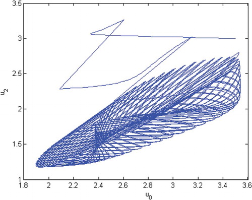
Now, to verify the correctness of Theorems 3.1–3.3, we consider system (24(24) $\begin{array}{rl}\frac{\mathrm{\partial }{u}_0}{\mathrm{\partial }t}& ={\mathcal{D}}_0\mathrm{\Delta }{u}_0+u_0\left(a_0(t,x)-b_0(t,x)u_0-\frac{c_1(t,x)u_1}{{\beta }_1(t,x)u_0+{\gamma }_1(t,x)u_1}\right.\\ & \left.-\frac{c_2(t,x)u_2}{{\beta }_2(t,x)u_0+{\gamma }_2(t,x)u_2}\right),\end{array}$(24) )–(28(28) ${\left.\frac{\mathrm{\partial }{u}_s}{\mathrm{\partial }n}\right|}_{\mathrm{\partial \Omega }}=0,s=0,1,\dots ,2.$(28) ) with $f_{0k}(x,u_0,u_1,u_2)\equiv 0.8$, $f_{1k}(x,u_0,u_1,u_2)\equiv 1.2$ and $f_{2k}(x,u_0,u_1,u_2)\equiv 0.7$ for all $k=1,2,\dots$. Choose ${\mathcal{D}}_0={\mathcal{D}}_1={\mathcal{D}}_2=1$, $a_0(t,x)=1.5\sin \left(t\right)+1.5\cos \left(x\right)+12$, $b_0(t,x)=\cos \left(t\right)+2\cos \left(x\right)+6$, $a_1(t,x)=0.1\sin \left(t\right)\cos \left(x\right)+0.4$, $b_1(t,x)=0.5\cos \left(t\right)+1.2\cos \left(x\right)+3.5$, $a_2(t,x)=0.5\cos \left(t\right)\cos \left(x\right)+1$, $c_1(t,x)=2\sin \left(t\right)+\sin \left(x\right)+7$, $c_2(t,x)=\sin \left(t\right)+0.5\sin \left(x\right)+4.5$, ${\beta }_1(t,x)={\beta }_2(t,x)\equiv 1$, ${\gamma }_1(t,x)\equiv 1.8$ and ${\gamma }_2(t,x)\equiv 3$. Obviously, all the parameters have a common period $\tau =2\pi$ with respect to t. Choosing an appropriate per length in the matlab procedure, we can calculate p=26. Then, we have that the parameters satisfy all conditions of Theorem 3.1, further $\begin{array}{rl}& \sum _{l=1}^p\ln \underset{x\in \mathrm{\Omega },(u_0,u_1,u_2)\in S}{inf}{f}_{0l}(x,u_0,u_1,u_2)+\tau \left(a_0^L-\frac{c_1^M}{{\gamma }_1^L}-\frac{c_2^M}{{\gamma }_2^L}\right)=3.2740>0,\\ & \sum _{l=1}^p\ln \underset{x\in \mathrm{\Omega },(u_0,u_1,u_2)\in S}{inf}{f}_{1l}(x,u_0,u_1,u_2)-a_1^M\tau =1.5988>0\end{array}$ and $\sum _{l=1}^p\ln \underset{x\in \mathrm{\Omega },(u_0,u_1,u_2)\in S}{inf}{f}_{2l}(x,u_0,u_1,u_2)+\tau \left(\frac{c_2^L}{{\beta }_2^M}-a_2^M\right)=0.1512>0,$ which satisfy the conditions (30(30) $\sum _{l=1}^p\ln \underset{x\in \mathrm{\Omega },(u_0,u_1,u_2)\in S}{inf}{f}_{0l}(x,u_0,u_1,u_2)+\tau \left(a_0^L-\frac{c_1^M}{{\gamma }_1^L}-\frac{c_2^M}{{\gamma }_2^L}\right)>0,$(30) )–(32(32) $\sum _{l=1}^p\ln \underset{x\in \mathrm{\Omega },(u_0,u_1,u_2)\in S}{inf}{f}_{2l}(x,u_0,u_1,u_2)+\tau \left(\frac{c_2^L}{{\beta }_2^M}-a_2^M\right)>0.$(32) ) of Theorem 3.2. Hence, all the conditions of Theorem 3.2 are satisfied, then, system (24(24) $\begin{array}{rl}\frac{\mathrm{\partial }{u}_0}{\mathrm{\partial }t}& ={\mathcal{D}}_0\mathrm{\Delta }{u}_0+u_0\left(a_0(t,x)-b_0(t,x)u_0-\frac{c_1(t,x)u_1}{{\beta }_1(t,x)u_0+{\gamma }_1(t,x)u_1}\right.\\ & \left.-\frac{c_2(t,x)u_2}{{\beta }_2(t,x)u_0+{\gamma }_2(t,x)u_2}\right),\end{array}$(24) )–(28(28) ${\left.\frac{\mathrm{\partial }{u}_s}{\mathrm{\partial }n}\right|}_{\mathrm{\partial \Omega }}=0,s=0,1,\dots ,2.$(28) ) is permanent. See Figures 1–5. Here, we choose $x\in \mathrm{\Omega }=[-2,2]$ and the initial conditions $u(0,x)=3.5,u_1(0,x)=4$ and $u_2(0,x)=3$ for all $x\in \mathrm{\Omega }$.

Figure 1. The permanence of species $u_0$.

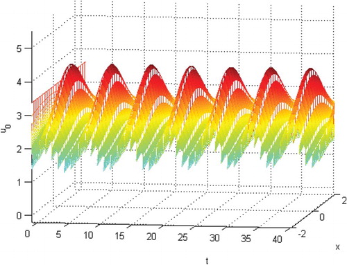
Figure 2. The permanence of species $u_1$.

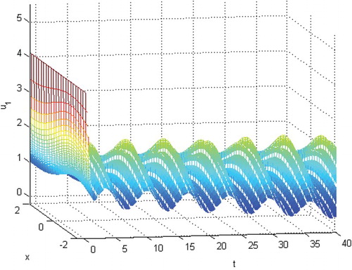
Figure 3. The permanence of species $u_2$.

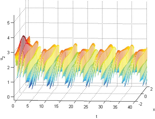
Figure 4. The phase of species $u_0$ and $u_1$.

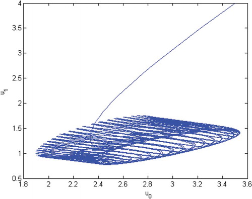
Figure 5. The phase of species $u_0$ and $u_2$.

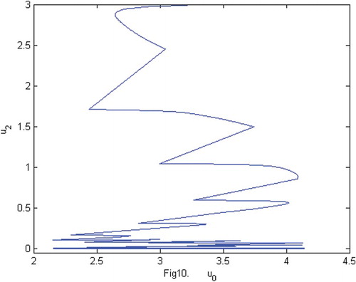
However, if we choose $a_1(t,x)=0.1\sin \left(t\right)\cos \left(x\right)+1.9$, $a_2(t,x)=0.5\cos \left(t\right)\cos \left(x\right)+1$, $c_1(t,x)=0.2\sin \left(t\right)+0.3\sin \left(x\right)+4.5$, ${\beta }_1(t,x)\equiv 5$, ${\beta }_2(t,x)\equiv 4$(the increase of the coefficients ${\beta }_1$ and ${\beta }_2$ implies the increase of the prey's defence capability), and other parameters are not changed. Then, we have that the parameters satisfy all the conditions of Theorem 3.1, further $\sum _{l=1}^p\ln \underset{x\in \mathrm{\Omega },(u_0,u_1,u_2)\in S}{sup}{f}_{1l}(x,u_0,u_1,u_2)+\tau \left(\frac{c_1^M}{{\beta }_1^L}-a_1^L\right)=-0.2862<0$ and $\sum _{l=1}^p\ln \underset{x\in \mathrm{\Omega },(u_0,u_1,u_2)\in S}{sup}{f}_{2l}(x,u_0,u_1,u_2)+\tau \left(\frac{c_2^M}{{\beta }_2^L}-a_2^L\right)=-2.9904<0,$ which satisfy the conditions (33(33) $\sum _{l=1}^p\ln \underset{x\in \mathrm{\Omega },(u_0,u_1,u_2)\in S}{sup}{f}_{1l}(x,u_0,u_1,u_2)+\tau \left(\frac{c_1^M}{{\beta }_1^L}-a_1^L\right)<0$(33) ) and (34(34) $\sum _{l=1}^p\ln \underset{x\in \mathrm{\Omega },(u_0,u_1,u_2)\in S}{sup}{f}_{2l}(x,u_0,u_1,u_2)+\tau \left(\frac{c_2^M}{{\beta }_2^L}-a_2^L\right)<0.$(34) ) of Theorem 3.3. Hence, all the conditions of Theorem 3.3 are satisfied, then, species $u_1$ and $u_2$ will be extinct. See Figures 7–10. From Figures 6, 9 and 10, we know that species $u_0$ is also permanent when species $u_1$ and $u_2$ approach to zero.

Figure 6. The permanence of species $u_0$ when $u_1\to 0,u_2\to 0$.

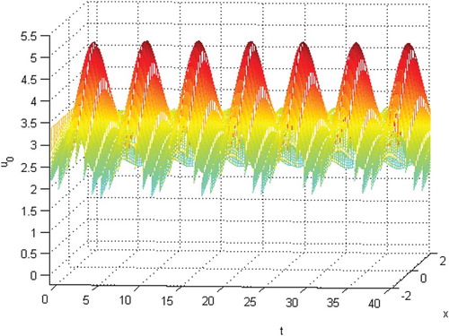
Figure 7. The extinction of species $u_1$.

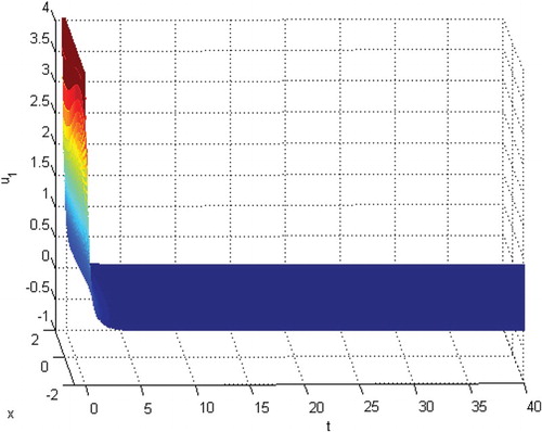
Figure 8. The extinction of species $u_2$.

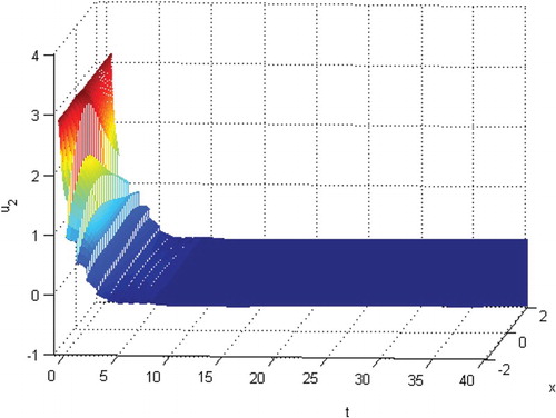
Figure 9. The phase of species $u_0$ and $u_1$.

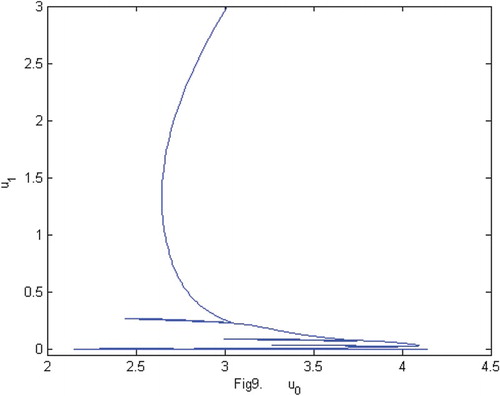
Figure 10. The phase of species $u_0$ and $u_2$.

6. Conclusion and discussion

In this paper, we present and study a one-prey-n-predator impulsive reaction-diffusion periodic predator–prey system with ratio-dependent functional response. The reaction-diffusion term shows that our prey and predator species are only confined in an isolated habitat for which the impact of migration, including both emigration and immigration, is presumably negligible, such as a remote patchy forest or an isolated island or a lake ecosystem which is practically water islands with distinct boundaries. Some sufficient conditions for the permanence (Theorems 3.1 and 3.2), extinction (Theorem 3.3) and the existence of a unique globally stable positive periodic solution (Theorem 4.1) of the system are established. By Theorem 3.1, we see that the prey species with intra-specific competition is ultimately bounded if the impulsive coefficients are bounded for any bounded solution of the system, so do the predator species which have the intra-specific competitions (Equation (2(2) $\frac{\mathrm{\partial }{u}_i}{\mathrm{\partial }t}={\mathcal{D}}_i\mathrm{\Delta }{u}_i+u_i\left(-a_i(t,x)-b_i(t,x)u_i+\frac{c_i(t,x)u_0}{{\beta }_i(t,x)u_0+{\gamma }_i(t,x)u_i}\right),i=1,\dots ,m,$(2) )). For each predator species without intra-specific competition (Equation (3(3) $\frac{\mathrm{\partial }{u}_j}{\mathrm{\partial }t}={\mathcal{D}}_j\mathrm{\Delta }{u}_j+u_j\left(-a_j(t,x)+\frac{c_j(t,x)u_0}{{\beta }_j(t,x)u_0+{\gamma }_j(t,x)u_j}\right),j=m+1,\dots ,n,$(3) )), its ultimate boundedness requires a negative average growth rate in a τ-period in the absent of the prey species by Theorem 3.1. By Theorem 3.2, we see that if the prey or predator species want to be permanent, a positive average growth rate in a τ-period must be satisfied. However, under the permanence of the prey species, the predator species are still extinct if their average growth rates in a τ-period are negative, which are shown by Theorem 3.3.

We note that if the system is permanent, by Theorem 4.1, it has a unique globally asymptotically stable strictly positive piecewise continuous τ-periodic solution if $\sum _{l=1}^p\ln K_l+\tau {\lambda }_M<0$. Thus, there is an interesting problem. If this system has a unique globally asymptotically stable strictly positive τ-periodic solution, the system should be permanent. It seems that Theorem 4.1 may imply Theorem 3.2. But unfortunately, we cannot claim it is true, since the condition $\sum _{l=1}^p\ln K_l+\tau {\lambda }_M<0$ in Theorem 4.1 is dependent of σ and N, which are determined by the bound of solutions when the system is permanent. Whether is there a unique globally asymptotically stable τ-periodic solution only if conditions (16(16) $\begin{array}{rl}& \sum _{l=1}^p\ln \underset{x\in \mathrm{\Omega },(u_0,u_1,\dots ,u_n)\in S}{inf}{f}_{0l}(x,u_0,u_1,\dots ,u_n)+\tau \left(a_0^L-\sum _{d=1}^n\frac{c_d^M}{{\gamma }_d^L}\right)>0,\end{array}$(16) ), (17(17) $\begin{array}{rl}& \sum _{l=1}^p\ln \underset{x\in \mathrm{\Omega },(u_0,u_1,\dots ,u_n)\in S}{inf}{f}_{il}(x,u_0,u_1,\dots ,u_n)-a_i^M\tau >0,i=1,2,\dots ,m\end{array}$(17) ) and (18(18) $\begin{array}{rl}& \sum _{l=1}^p\ln \underset{x\in \mathrm{\Omega },(u_0,u_1,\dots ,u_n)\in S}{inf}{f}_{jl}(x,u_0,u_1,\dots ,u_n)+\tau \left(\frac{c_j^L}{{\beta }_j^M}-a_j^M\right)>0,\\ & j=m+1,m+2,\dots ,n\end{array}$(18) ) hold (the system is permanent)? Can we find other conditions independent of σ and N that can guarantee the existence of the unique globally stable τ-periodic solution? We will continue to study these problems in the future.

In this paper, we only studied the system with ratio-dependent functional response, whether other type functional responses such as Holling type II, Holling type III and Beddington-DeAnglis functional response can be discussed with the same methods or not, still remain open problems.

Disclosure statement

No potential conflict of interest was reported by the authors.

Additional information

Funding

This work was supported by the National Natural Science Foundation of China [grant numbers 11401060, 11401061, 11401117, 11401217, 11501065], the Basic and Advanced Research Project of Chongqing [grant numbers cstc2016jcyjA0412, cstc2017jcyjAX0131, cstc2015jcyjA00033], the Science and Technology Commission of Shanghai Municipality (STCSM) [grant number 13dz2260400] and the Program of Chongqing Innovation Team Project in University [grant number CXTDX201601022].

References

- B. Ainsebaa and S. Aniţa, Internal stabilizability for a reaction-diffusion problem modeling a predator–prey system, Nonlinear Anal. 61 (2005), pp. 491–501. doi: 10.1016/j.na.2004.09.055
- M.U. Akhmet, M. Beklioglu, T. Ergenc, and V.I. Tkachenko, An impulsive ratio-dependent predator–prey system with diffusion, Nonlinear Anal. RWA 7 (2006), pp. 1255–1267. doi: 10.1016/j.nonrwa.2005.11.007
- Z. Du and Z. Feng, Periodic solutions of a neutral impulsive predator–prey model with Beddington-DeAngelis functional response with delays, J. Comput. Appl. Math. 258 (2014), pp. 87–98. doi: 10.1016/j.cam.2013.09.008
- C. Duque, K. Kiss, and M. Lizana, On the dynamics of an n-dimensional ratio-dependent predator–prey system with diffusion, Appl. Math. Comput. 208 (2009), pp. 98–105.
- R.A. Fisher, The wave of advance of advantageous genes, Ann. Eugenics 7 (1937), pp. 353–369.
- Z. Ge and Y. He, Diffusion effect and stability analysis of a predator–prey system described by a delayed reaction-diffusion equations, J. Math. Anal. Appl. 339 (2008), pp. 1432–1450. doi: 10.1016/j.jmaa.2007.07.060
- A. Kolmogoroff, I. Petrovsky, and N. Piscounoff, Study of the diffusion equation with growth of the quantity of matter and its application to a biological problem, Moscow Univ. Bull. Math. 1 (1937), pp. 1–25.
- V. Lakshmikantham, D. Bainov, and P. Simenov, Theory of Impulsive Differential Equations, World Scientific, Singapore, 1989.
- X. Liu and L. Chen, Global dynamics of the periodic logistic system with periodic impulsive perturbations, J. Math. Anal. Appl. 289 (2004), pp. 279–291. doi: 10.1016/j.jmaa.2003.09.058
- C.V. Pao, Nonlinear Parabolic and Elliptic Equations, Plenum, New York, 1992.
- A.M. Samoilenko and N.A. Perestyuk, Impulsive Differential Equations, World Scientific, Singapore, 1995.
- H.B. Shi and Y. Li, Global asymptotic stability of a diffusive predator–prey model with ratio-dependent functional response, Appl. Math. Comput. 250 (2015), pp. 71–77.
- J. Shi and R. Shivaji, Persistence in reaction-diffusion models with weak allee effect, J. Math. Biol. 52 (2006), pp. 807–829. doi: 10.1007/s00285-006-0373-7
- J.G. Skellam, Random dispersal in theoretical populations, Biometrika 38 (1951), pp. 196–218. doi: 10.1093/biomet/38.1-2.196
- L.H. Smith, Dynamics of Competition, Lecture Notes in Mathematics, Vol. 1714, Springer, Berlin, 1999, pp. 192–240.
- W. Walter, Differential inequalities and maximum principles; theory, new methods and applications, Nonlinear Anal. Appl. 30 (1997), pp. 4695–4711. doi: 10.1016/S0362-546X(96)00259-3
- C. Wang, Rich dynamics of a predator–prey model with spatial motion, Appl. Math. Comput. 260 (2015), pp. 1–9.
- Q. Wang, Z. Wang, Y. Wang, H. Zhang, and M. Ding, An impulsive ratio-dependent n+1-species predator–prey model with diffusion, Nonlinear Anal. RWA 11 (2010), pp. 2164–2174. doi: 10.1016/j.nonrwa.2009.11.013
- R. Wu, X. Zou, and K. Wang, Asymptotic behavior of a stochastic non-autonomous predator–prey model with impulsive perturbations, Commun. Nonlinear Sci. Numer. Simul. 20 (2015), pp. 965–974. doi: 10.1016/j.cnsns.2014.06.023
- R. Xu, A reaction-diffusion predator–prey model with stage structure and nonlocal delay, Appl. Math. Comput. 175 (2006), pp. 984–1006.
- R. Xu and Z. Ma, Global stability of a reaction-diffusion predator–prey model with a nonlocal delay, Math. Comput. Model. 50 (2009), pp. 194–206. doi: 10.1016/j.mcm.2009.02.011
- Y. Yu, W. Deng, and Y. Wu, Positivity and boundedness preserving schemes for space-time fractional predator–prey reaction-diffusion model, Comput. Math. Appl. 69 (2015), pp. 743–759. doi: 10.1016/j.camwa.2015.02.024
- Z. Zhao and X. Wu, Nonlinear analysis of a delayed stage-structured predator–prey model with impulsive effect and environment pollution, Appl. Math. Comput. 232 (2014), pp. 1262–1268.
- H. Zhang, L. Chen, and J.J. Nieto, A delayed epidemic model with stage-structure and pulses for management strategy, Nonlinear Anal. RWA 9 (2008), pp. 1714–1726. doi: 10.1016/j.nonrwa.2007.05.004