Dynamics of malaria transmission model with sterile mosquitoes

ABSTRACT

In this paper, a malaria transmission model with sterile mosquitoes is considered. We first formulate a simple SEIR malaria transmission model as our baseline model. Then sterile mosquitoes are introduced into the baseline model. We consider the case that the release rate of sterile mosquitoes is proportional to the wild mosquito population size. To investigate the impact of releasing sterile mosquitoes on the malaria transmission, the dynamics of the baseline model and the models with the sterile mosquitoes are discussed. We derive formulas of the reproductive numbers and explore the existence of endemic equilibrium as the reproductive number is more than unity for these models. It is shown that both the baseline model and the models with the sterile mosquitoes undergo backward bifurcations. Based on theoretical analysis and numerical simulation, we investigate the impact of releasing sterile mosquitoes on malaria transmission.

KEYWORDS:

• Sterile mosquito
• stability
• backward bifurcation
• malaria model

AMS SUBJECT CLASSIFICATIONS:

• 34C60
• 34D99
• 92D25
• 92D30
• 92D40

1. Introduction

The sterile insect technique is a method of controlling mosquitoes. It has been proved to be useful and effective. Utilizing radiological, chemical, physical, or transgenic methods male mosquitoes are modified to be sterile so they are incapable of producing offspring despite mating. These sterile male mosquitoes are then released into the environment to mate with the wild mosquitoes that are present in the environment. Wild females generally only mate once in their lifetime, thus if they mate with a sterile male, they will either not reproduce, or produce eggs, but the eggs will not hatch. Repeated releases of genetically modified mosquitoes or releasing a significantly large number of sterile mosquitoes may eventually wipe out a wild mosquito population, although it is often more realistic to consider controlling the population rather than eradicating it [1,3,4,17–19].

Mathematical models have been formulated in the literature to study the interactive dynamics and control of the wild and sterile mosquito populations [5–10,15,16]. In particular, models incorporating different strategies in releasing sterile mosquitoes have been formulated and studied in [6,12,13]. The impact of releasing sterile mosquitoes on the malaria transmission has been studied in [20]. However, only the case that the release rate of sterile mosquitoes is constant was considered in [20]. In fact, there are different strategies for releasing sterile mosquitoes and different strategies have different impact on the wild mosquitoes. For the case of constant releases, even though wild mosquitoes go extinct, there are still sterile mosquitoes around. This is due to the constant releases of sterile mosquitoes no matter whether the wild mosquito population size is large or small. This apparently does not seem to be the best strategy economically. As in [6,12,13], to have a more optimal and economically effective strategy for releasing sterile mosquitoes in an area where the population size of wild mosquitoes is relatively small, instead of keeping the release rate constantly fixed, we may let the release rate be proportional to the population size of the wild mosquitoes.

In this paper, we assume that the Anopheles gambiae is the sole malaria-disease vector in the area. To have a better understanding of the impact of releasing sterile mosquitoes on the malaria transmission and provide useful guidance for good strategies for releasing sterile mosquitoes, we focus on the impact of releases of sterile mosquitoes on malaria transmission when the number of releases is proportional to the population size of the wild mosquitoes. The malaria model in this paper is suitable for all malaria which transmits between human and mosquitoes, such as the malaria transmitted by Plasmodium vivax, Plasmodium ovale, Plasmodium malariae and Plasmodium falciparum. First, we consider a simple SEIR malaria transmission model as our baseline model in Section 2. We derive formulas of the reproductive numbers and prove the existence of an endemic equilibrium for the baseline models, and the occurrence of a backward bifurcation is consider. We then introduce the sterile mosquitoes into the baseline malaria model where the susceptible mosquitoes consist of the wild and sterile mosquitoes in Section 3. We consider the case where the release rate of sterile mosquitoes is proportional to the population size of the wild mosquitoes. The reproductive numbers, the existence of an endemic equilibrium and a backward bifurcation for the models with sterile mosquitoes are discussed. In Section 4, we provide some examples and simulations to illustrate our theoretical results. The impact of sterile mosquitoes on malaria transmission is investigated. We finally give brief discussions in Section 5.

2. Baseline model for malaria transmission

As in [20], we consider a simple SEIR malaria model as our baseline model [2,10,11]. We divide the total human population, denoted by $N_h$, into the following subclasses: susceptible $S_h$, latent $E_h$, infective $I_h$ and recovered $R_h$. So that $N_h=S_h+E_h+I_h+R_h$. The total mosquito population, denoted by $N_v$, is divided into susceptible mosquitoes$S_v$, latent mosquitoes$E_v$ and infective mosquitoes $I_v$. That is $N_v=S_v+E_v+I_v$.

Based on the works in [11,12], malaria transmission models were formulated in [20]. The schematics diagram of transmission of malaria is shown in Figure 1. The model equations for humans have the form (1) $\begin{array}{rl}\frac{\mathrm{d}{S}_h}{\mathrm{d}t}& ={\mathrm{\Lambda }}_h-({\mu }_h+{\lambda }_h)S_h+{\theta }_h{R}_h,\\ \frac{\mathrm{d}{E}_h}{\mathrm{d}t}& ={\lambda }_h{S}_h-({\mu }_h+{\gamma }_h)E_h,\\ \frac{\mathrm{d}{I}_h}{\mathrm{d}t}& ={\gamma }_h{E}_h-({\mu }_h+{\delta }_h+{\eta }_h)I_h,\\ \frac{\mathrm{d}{R}_h}{\mathrm{d}t}& ={\eta }_h{I}_h-({\mu }_h+{\theta }_h)R_h,\end{array}$(1) where ${\mathrm{\Lambda }}_h$ is the input flow of the susceptible humans, ${\mu }_h$ and ${\delta }_h$ are the natural and disease-induced death rates for humans, respectively, ${\lambda }_h$ is the infection rate or the incidence of infection from an infective mosquito to a susceptible human, and ${\gamma }_h$ is the developing rate of incubating humans to become infectious, such that $1/{\gamma }_h$ is the incubation period. We assume that the infectious can recover by drug administration or natural immunity by rate ${\eta }_h$, then part of the infectious will come into the recovery compartment. We also assume that the recovered people have partial immunity against malaria and will lose the immunity by rate ${\theta }_h$, then part of the recovered people will come into the susceptible compartment [14]. Notice that if there is no infection, the human population has an asymptotically stable steady state such that $\underset{t\to \mathrm{\infty }}{lim}{S}_h={\mathrm{\Lambda }}_h/{\mu }_h$. And the model equations for the mosquitoes have the form (2) $\begin{array}{rl}\frac{\mathrm{d}{S}_v}{\mathrm{d}t}& =C\left(N_v\right){\alpha }_v(1-{\xi }_v{N}_v)N_v-({\mu }_v+{\lambda }_v)S_v,\\ \frac{\mathrm{d}{E}_v}{\mathrm{d}t}& ={\lambda }_v{S}_v-({\mu }_v+{\gamma }_v)E_v,\\ \frac{\mathrm{d}{I}_v}{\mathrm{d}t}& ={\gamma }_v{E}_v-{\mu }_v{I}_v,\end{array}$(2) where $C\left(N_v\right)$ is the mating rate, ${\alpha }_v$ is the number of wild offspring produced per mate (where wild offspring refers to adult mosquitoes, not to eggs or larvae), ${\xi }_v$ is the carrying capacity parameter such that $1-{\xi }_v{N}_v$ describes the density dependent survival probability, ${\mu }_v$ is the natural death rate of the mosquitoes, ${\gamma }_v$ is the rate of incubating mosquitoes becoming infectious; that is, $1/{\gamma }_v$ is the extrinsic incubation period of the parasite within the mosquito or the period of sporogony, and ${\lambda }_v$ is the infection rate from an infective human to a susceptible mosquito. As in [12], we assume $r_0:={\alpha }_v-{\mu }_v>0$. The infection rates are given by (3) ${\lambda }_v=r{\beta }_h\frac{I_h}{N_h},$(3) and (4) ${\lambda }_h={\beta }_{v}r\frac{N_v}{N_h}\frac{I_v}{N_v}=r{\beta }_v\frac{I_v}{N_h},$(4) where r is the number of bites on humans by a single mosquito per unit of time, ${\beta }_h$ is the transmission probability per bite to a mosquito from an infective human, and ${\beta }_v$ is the transmission probability from an infective mosquito to a susceptible human per infected bite.

Figure 1. The compartmental model for malaria transmission.

In this paper, the mating rate is assumed to be a saturated function and takes the form of $C\left(N_v\right)=c{N}_v/(1+N_v)$. After we merge c into the parameter ${\alpha }_v$ and still denote it as ${\alpha }_v$, system (2(2) $\begin{array}{rl}\frac{\mathrm{d}{S}_v}{\mathrm{d}t}& =C\left(N_v\right){\alpha }_v(1-{\xi }_v{N}_v)N_v-({\mu }_v+{\lambda }_v)S_v,\\ \frac{\mathrm{d}{E}_v}{\mathrm{d}t}& ={\lambda }_v{S}_v-({\mu }_v+{\gamma }_v)E_v,\\ \frac{\mathrm{d}{I}_v}{\mathrm{d}t}& ={\gamma }_v{E}_v-{\mu }_v{I}_v,\end{array}$(2) ) becomes (5) $\begin{array}{rl}\frac{\mathrm{d}{S}_v}{\mathrm{d}t}& =\frac{{\alpha }_v{N}_v}{1+N_v}(1-{\xi }_v{N}_v)N_v-({\mu }_v+{\lambda }_v)S_v,\\ \frac{\mathrm{d}{E}_v}{\mathrm{d}t}& ={\lambda }_v{S}_v-({\mu }_v+{\gamma }_v)E_v,\\ \frac{\mathrm{d}{I}_v}{\mathrm{d}t}& ={\gamma }_v{E}_v-{\mu }_v{I}_v.\end{array}$(5) Clearly, the total population of mosquitoes satisfies the following equation (6) $\frac{\mathrm{d}{N}_v}{\mathrm{d}t}=\frac{{\alpha }_v{N}_v}{1+N_v}(1-{\xi }_v{N}_v)N_v-{\mu }_v{N}_v.$(6) From [12], if $r_0>2\sqrt{{\alpha }_v{\xi }_v{\mu }_v}$, Equation (5(5) $\begin{array}{rl}\frac{\mathrm{d}{S}_v}{\mathrm{d}t}& =\frac{{\alpha }_v{N}_v}{1+N_v}(1-{\xi }_v{N}_v)N_v-({\mu }_v+{\lambda }_v)S_v,\\ \frac{\mathrm{d}{E}_v}{\mathrm{d}t}& ={\lambda }_v{S}_v-({\mu }_v+{\gamma }_v)E_v,\\ \frac{\mathrm{d}{I}_v}{\mathrm{d}t}& ={\gamma }_v{E}_v-{\mu }_v{I}_v.\end{array}$(5) ) has two positive equilibria (7) $N_v^{\pm }:=\frac{r_0\pm \sqrt{r_0^2-4{\alpha }_v{\xi }_v{\mu }_v}}{2{\alpha }_v{\xi }_v},$(7) and positive equilibrium $N_v^{-}$ is unstable, $N_v^{+}$ is asymptotically stable. Instead of system (5(5) $\begin{array}{rl}\frac{\mathrm{d}{S}_v}{\mathrm{d}t}& =\frac{{\alpha }_v{N}_v}{1+N_v}(1-{\xi }_v{N}_v)N_v-({\mu }_v+{\lambda }_v)S_v,\\ \frac{\mathrm{d}{E}_v}{\mathrm{d}t}& ={\lambda }_v{S}_v-({\mu }_v+{\gamma }_v)E_v,\\ \frac{\mathrm{d}{I}_v}{\mathrm{d}t}& ={\gamma }_v{E}_v-{\mu }_v{I}_v.\end{array}$(5) ), we consider the following system for the mosquito part in the baseline model (8) $\begin{array}{rl}\frac{\mathrm{d}{N}_v}{\mathrm{d}t}& =\frac{{\alpha }_v{N}_v}{1+N_v}(1-{\xi }_v{N}_v)N_v-{\mu }_v{N}_v,\\ \frac{\mathrm{d}{E}_v}{\mathrm{d}t}& ={\lambda }_v(N_v-E_v-I_v)-({\mu }_v+{\gamma }_v)E_v,\\ \frac{\mathrm{d}{I}_v}{\mathrm{d}t}& ={\gamma }_v{E}_v-{\mu }_v{I}_v.\end{array}$(8) Define $\mathrm{\Omega }:=\left\{\right(N_h,N_v):0\le N_h\le N_h^0,0\le N_v\le N_v^{+}\},$ where $N_h^0={\mathrm{\Lambda }}_h/{\mu }_h$ and $N_v^{+}$ is given by (7(7) $N_v^{\pm }:=\frac{r_0\pm \sqrt{r_0^2-4{\alpha }_v{\xi }_v{\mu }_v}}{2{\alpha }_v{\xi }_v},$(7) ). Then the region Ω is a positive invariant set for system (1(1) $\begin{array}{rl}\frac{\mathrm{d}{S}_h}{\mathrm{d}t}& ={\mathrm{\Lambda }}_h-({\mu }_h+{\lambda }_h)S_h+{\theta }_h{R}_h,\\ \frac{\mathrm{d}{E}_h}{\mathrm{d}t}& ={\lambda }_h{S}_h-({\mu }_h+{\gamma }_h)E_h,\\ \frac{\mathrm{d}{I}_h}{\mathrm{d}t}& ={\gamma }_h{E}_h-({\mu }_h+{\delta }_h+{\eta }_h)I_h,\\ \frac{\mathrm{d}{R}_h}{\mathrm{d}t}& ={\eta }_h{I}_h-({\mu }_h+{\theta }_h)R_h,\end{array}$(1) ) and (8(8) $\begin{array}{rl}\frac{\mathrm{d}{N}_v}{\mathrm{d}t}& =\frac{{\alpha }_v{N}_v}{1+N_v}(1-{\xi }_v{N}_v)N_v-{\mu }_v{N}_v,\\ \frac{\mathrm{d}{E}_v}{\mathrm{d}t}& ={\lambda }_v(N_v-E_v-I_v)-({\mu }_v+{\gamma }_v)E_v,\\ \frac{\mathrm{d}{I}_v}{\mathrm{d}t}& ={\gamma }_v{E}_v-{\mu }_v{I}_v.\end{array}$(8) ). We assume $(N_h,N_v)\in \mathrm{\Omega }$.

By investigating the local stability of the infection-free equilibrium, we define the reproductive number of infection for system (1(1) $\begin{array}{rl}\frac{\mathrm{d}{S}_h}{\mathrm{d}t}& ={\mathrm{\Lambda }}_h-({\mu }_h+{\lambda }_h)S_h+{\theta }_h{R}_h,\\ \frac{\mathrm{d}{E}_h}{\mathrm{d}t}& ={\lambda }_h{S}_h-({\mu }_h+{\gamma }_h)E_h,\\ \frac{\mathrm{d}{I}_h}{\mathrm{d}t}& ={\gamma }_h{E}_h-({\mu }_h+{\delta }_h+{\eta }_h)I_h,\\ \frac{\mathrm{d}{R}_h}{\mathrm{d}t}& ={\eta }_h{I}_h-({\mu }_h+{\theta }_h)R_h,\end{array}$(1) ) and (8(8) $\begin{array}{rl}\frac{\mathrm{d}{N}_v}{\mathrm{d}t}& =\frac{{\alpha }_v{N}_v}{1+N_v}(1-{\xi }_v{N}_v)N_v-{\mu }_v{N}_v,\\ \frac{\mathrm{d}{E}_v}{\mathrm{d}t}& ={\lambda }_v(N_v-E_v-I_v)-({\mu }_v+{\gamma }_v)E_v,\\ \frac{\mathrm{d}{I}_v}{\mathrm{d}t}& ={\gamma }_v{E}_v-{\mu }_v{I}_v.\end{array}$(8) ) as (9) $R_0:=\sqrt{\frac{r^2{\beta }_h{\beta }_v{\gamma }_h{\gamma }_v{N}_v^{+}}{({\mu }_h+{\gamma }_h)({\mu }_h+{\delta }_h+{\eta }_h)({\mu }_v+{\gamma }_v){\mu }_v{N}_h^0}}.$(9)

We further write $\begin{array}{rl}{K}_1& :=\frac{1}{{\mu }_h}-{\theta }_h\frac{{\eta }_h{\gamma }_h}{{\mu }_h{\sigma }_1{\sigma }_2{\sigma }_3},K_2:=\frac{{\sigma }_2{\sigma }_3+{\sigma }_3{\gamma }_h+{\gamma }_h{\eta }_h}{{\sigma }_1{\sigma }_2{\sigma }_3},\\ B_1& :=\frac{r{\beta }_h{\gamma }_h}{{\sigma }_1{\sigma }_2},K_3:=K_2+\frac{B_1}{{\mu }_v},\end{array}$ and (10) $R_0^{\ast }:=\frac{{\left(K_1\right(K_2+K_3)-2K_2{K}_3+2\sqrt{K_2{K}_3(K_2-K_1)(K_3-K_1)})}^{1/2}}{K_1},$(10)

then we have the following theorem for system (1(1) $\begin{array}{rl}\frac{\mathrm{d}{S}_h}{\mathrm{d}t}& ={\mathrm{\Lambda }}_h-({\mu }_h+{\lambda }_h)S_h+{\theta }_h{R}_h,\\ \frac{\mathrm{d}{E}_h}{\mathrm{d}t}& ={\lambda }_h{S}_h-({\mu }_h+{\gamma }_h)E_h,\\ \frac{\mathrm{d}{I}_h}{\mathrm{d}t}& ={\gamma }_h{E}_h-({\mu }_h+{\delta }_h+{\eta }_h)I_h,\\ \frac{\mathrm{d}{R}_h}{\mathrm{d}t}& ={\eta }_h{I}_h-({\mu }_h+{\theta }_h)R_h,\end{array}$(1) ) and (8(8) $\begin{array}{rl}\frac{\mathrm{d}{N}_v}{\mathrm{d}t}& =\frac{{\alpha }_v{N}_v}{1+N_v}(1-{\xi }_v{N}_v)N_v-{\mu }_v{N}_v,\\ \frac{\mathrm{d}{E}_v}{\mathrm{d}t}& ={\lambda }_v(N_v-E_v-I_v)-({\mu }_v+{\gamma }_v)E_v,\\ \frac{\mathrm{d}{I}_v}{\mathrm{d}t}& ={\gamma }_v{E}_v-{\mu }_v{I}_v.\end{array}$(8) ).

Theorem 2.1

1. The infection-free equilibrium $(N_h^0,0,0,0,0,0,N_v^{+})$ is locally asymptotically stable if $R_0<1$ and unstable if $R_0>1$. There exists a unique endemic equilibrium if $R_0>1$.

2. With the condition $K_2+K_3<K_1$, there exists a subthreshold, $0<R_0^{\ast }<1$, given in (10(10) $R_0^{\ast }:=\frac{{\left(K_1\right(K_2+K_3)-2K_2{K}_3+2\sqrt{K_2{K}_3(K_2-K_1)(K_3-K_1)})}^{1/2}}{K_1},$(10) ), such that system (1(1) $\begin{array}{rl}\frac{\mathrm{d}{S}_h}{\mathrm{d}t}& ={\mathrm{\Lambda }}_h-({\mu }_h+{\lambda }_h)S_h+{\theta }_h{R}_h,\\ \frac{\mathrm{d}{E}_h}{\mathrm{d}t}& ={\lambda }_h{S}_h-({\mu }_h+{\gamma }_h)E_h,\\ \frac{\mathrm{d}{I}_h}{\mathrm{d}t}& ={\gamma }_h{E}_h-({\mu }_h+{\delta }_h+{\eta }_h)I_h,\\ \frac{\mathrm{d}{R}_h}{\mathrm{d}t}& ={\eta }_h{I}_h-({\mu }_h+{\theta }_h)R_h,\end{array}$(1) ) and (8(8) $\begin{array}{rl}\frac{\mathrm{d}{N}_v}{\mathrm{d}t}& =\frac{{\alpha }_v{N}_v}{1+N_v}(1-{\xi }_v{N}_v)N_v-{\mu }_v{N}_v,\\ \frac{\mathrm{d}{E}_v}{\mathrm{d}t}& ={\lambda }_v(N_v-E_v-I_v)-({\mu }_v+{\gamma }_v)E_v,\\ \frac{\mathrm{d}{I}_v}{\mathrm{d}t}& ={\gamma }_v{E}_v-{\mu }_v{I}_v.\end{array}$(8) ) has no endemic equilibrium if $R_0<R_0^{\ast }$, a unique endemic equilibrium if $R_0=R_0^{\ast }$, and two endemic equilibria, which implies a backward bifurcation, if $R_0^{\ast }<R_0<1$.

3. On the other hand, if $K_2+K_3\ge K_1$, there exists no endemic equilibrium, and backward bifurcation cannot occur for $R_0<1$.

The detailed proof of this theorem is given in the appendix.

3. The models with sterile mosquitoes

Now we introduce the sterile mosquito population into the baseline model. The part of the model equations for humans is the same as in system (1(1) $\begin{array}{rl}\frac{\mathrm{d}{S}_h}{\mathrm{d}t}& ={\mathrm{\Lambda }}_h-({\mu }_h+{\lambda }_h)S_h+{\theta }_h{R}_h,\\ \frac{\mathrm{d}{E}_h}{\mathrm{d}t}& ={\lambda }_h{S}_h-({\mu }_h+{\gamma }_h)E_h,\\ \frac{\mathrm{d}{I}_h}{\mathrm{d}t}& ={\gamma }_h{E}_h-({\mu }_h+{\delta }_h+{\eta }_h)I_h,\\ \frac{\mathrm{d}{R}_h}{\mathrm{d}t}& ={\eta }_h{I}_h-({\mu }_h+{\theta }_h)R_h,\end{array}$(1) ). We let $S_g$ be the number of sterile mosquitoes and $B\left(N_v\right)$ be the rate of releases. Then the part of the mosquitoes in the disease transmission model is given by the system (11) $\begin{array}{rl}\frac{\mathrm{d}{S}_v}{\mathrm{d}t}& =\frac{{\alpha }_v{N}_v}{1+N_v+S_g}(1-{\xi }_v{N}_v)N_v-({\mu }_v+{\lambda }_v)S_v,\\ \frac{\mathrm{d}{E}_v}{\mathrm{d}t}& ={\lambda }_v{S}_v-({\mu }_v+{\gamma }_v)E_v,\\ \frac{\mathrm{d}{I}_v}{\mathrm{d}t}& ={\gamma }_v{E}_v-{\mu }_v{I}_v,\\ \frac{\mathrm{d}{S}_g}{\mathrm{d}t}& =B\left(N_v\right)-{\mu }_v{S}_g,\end{array}$(11) where we assume the wild mosquitoes have the same death rate as sterile mosquitoes.

Let $N_v=S_v+E_v+I_v$, then we have $\frac{\mathrm{d}{N}_v}{\mathrm{d}t}=\frac{{\alpha }_v{N}_v}{1+N_v+S_g}(1-{\xi }_v{N}_v)N_v-{\mu }_v{N}_v.$ Thus, instead of system (11(11) $\begin{array}{rl}\frac{\mathrm{d}{S}_v}{\mathrm{d}t}& =\frac{{\alpha }_v{N}_v}{1+N_v+S_g}(1-{\xi }_v{N}_v)N_v-({\mu }_v+{\lambda }_v)S_v,\\ \frac{\mathrm{d}{E}_v}{\mathrm{d}t}& ={\lambda }_v{S}_v-({\mu }_v+{\gamma }_v)E_v,\\ \frac{\mathrm{d}{I}_v}{\mathrm{d}t}& ={\gamma }_v{E}_v-{\mu }_v{I}_v,\\ \frac{\mathrm{d}{S}_g}{\mathrm{d}t}& =B\left(N_v\right)-{\mu }_v{S}_g,\end{array}$(11) ), we consider the following system for the mosquito part in the disease transmission model (12) $\begin{array}{rl}\frac{\mathrm{d}{N}_v}{\mathrm{d}t}& =\frac{{\alpha }_v{N}_v}{1+N_v+S_g}(1-{\xi }_v{N}_v)N_v-{\mu }_v{N}_v,\\ \frac{\mathrm{d}{E}_v}{\mathrm{d}t}& ={\lambda }_v(N_v-E_v-I_v)-({\mu }_v+{\gamma }_v)E_v,\\ \frac{\mathrm{d}{I}_v}{\mathrm{d}t}& ={\gamma }_v{E}_v-{\mu }_v{I}_v,\\ \frac{\mathrm{d}{S}_g}{\mathrm{d}t}& =B\left(N_v\right)-{\mu }_v{S}_g.\end{array}$(12) To have a more economically effective strategy for releases of sterile mosquitoes in an area where the population size of wild mosquitoes is relatively small, we let the number of releases be proportional to the population size of the wild mosquitoes such that $B\left(N_v\right):=b{N}_v$. It is clear that the interactive dynamics between the total wild and sterile mosquitoes are governed by the following system (13) $\begin{array}{rl}\frac{\mathrm{d}{N}_v}{\mathrm{d}t}& =\frac{{\alpha }_v{N}_v}{1+N_v+S_g}(1-{\xi }_v{N}_v)N_v-{\mu }_v{N}_v,\\ \frac{\mathrm{d}{S}_g}{\mathrm{d}t}& =b{N}_v-{\mu }_v{S}_g,\end{array}$(13) and from [12] the results for system (13(13) $\begin{array}{rl}\frac{\mathrm{d}{N}_v}{\mathrm{d}t}& =\frac{{\alpha }_v{N}_v}{1+N_v+S_g}(1-{\xi }_v{N}_v)N_v-{\mu }_v{N}_v,\\ \frac{\mathrm{d}{S}_g}{\mathrm{d}t}& =b{N}_v-{\mu }_v{S}_g,\end{array}$(13) ) are

Lemma 3.1

Theorem 4.1 [12]

The origin (0,0) is a trivial equilibrium of system (13(13) $\begin{array}{rl}\frac{\mathrm{d}{N}_v}{\mathrm{d}t}& =\frac{{\alpha }_v{N}_v}{1+N_v+S_g}(1-{\xi }_v{N}_v)N_v-{\mu }_v{N}_v,\\ \frac{\mathrm{d}{S}_g}{\mathrm{d}t}& =b{N}_v-{\mu }_v{S}_g,\end{array}$(13) ), which is always locally asymptotically stable. Assume $r_0>2\sqrt{{\alpha }_v{\xi }_v{\mu }_v}$. Then system (13(13) $\begin{array}{rl}\frac{\mathrm{d}{N}_v}{\mathrm{d}t}& =\frac{{\alpha }_v{N}_v}{1+N_v+S_g}(1-{\xi }_v{N}_v)N_v-{\mu }_v{N}_v,\\ \frac{\mathrm{d}{S}_g}{\mathrm{d}t}& =b{N}_v-{\mu }_v{S}_g,\end{array}$(13) ) has no, one, or two positive equilibria if $b>b_c^p$, $b=b_c^p$, or $b<b_c^p$, respectively, where the release threshold $b_c^p$ is given by (14) $b_c^p:=r_0-2\sqrt{{\alpha }_v{\xi }_v{\mu }_v}.$(14) If there exist two positive equilibria,$E_p^{-}=(N_{vp}^{-},b{N}_{vp}^{-}/{\mu }_v)$ and $E_p^{+}=(N_{vp}^{+},b{N}_{vp}^{+}/{\mu }_v)$, where (15) $N_{vp}^{\pm }=\frac{r_0-b\pm \sqrt{(r_0-b{)}^2-4{\alpha }_v{\xi }_v{\mu }_v}}{2{\alpha }_v{\xi }_v}.$(15) $E_p^{-}$ is an unstable saddle and $E_p^{+}$ is a locally asymptotically stable node or spiral.

3.1. The reproductive number

Now the Jacobian matrix of system (1(1) $\begin{array}{rl}\frac{\mathrm{d}{S}_h}{\mathrm{d}t}& ={\mathrm{\Lambda }}_h-({\mu }_h+{\lambda }_h)S_h+{\theta }_h{R}_h,\\ \frac{\mathrm{d}{E}_h}{\mathrm{d}t}& ={\lambda }_h{S}_h-({\mu }_h+{\gamma }_h)E_h,\\ \frac{\mathrm{d}{I}_h}{\mathrm{d}t}& ={\gamma }_h{E}_h-({\mu }_h+{\delta }_h+{\eta }_h)I_h,\\ \frac{\mathrm{d}{R}_h}{\mathrm{d}t}& ={\eta }_h{I}_h-({\mu }_h+{\theta }_h)R_h,\end{array}$(1) ) and (12(12) $\begin{array}{rl}\frac{\mathrm{d}{N}_v}{\mathrm{d}t}& =\frac{{\alpha }_v{N}_v}{1+N_v+S_g}(1-{\xi }_v{N}_v)N_v-{\mu }_v{N}_v,\\ \frac{\mathrm{d}{E}_v}{\mathrm{d}t}& ={\lambda }_v(N_v-E_v-I_v)-({\mu }_v+{\gamma }_v)E_v,\\ \frac{\mathrm{d}{I}_v}{\mathrm{d}t}& ={\gamma }_v{E}_v-{\mu }_v{I}_v,\\ \frac{\mathrm{d}{S}_g}{\mathrm{d}t}& =B\left(N_v\right)-{\mu }_v{S}_g.\end{array}$(12) ) at an equilibrium $(S_h,R_h,I_h,E_h,I_v,E_v,N_v,S_g)$ is given by $\left(\begin{array}{cc}\tilde{J}& \cdot \\ 0& J_{33}\end{array}\right),$ where $J_{33}$ is the Jacobian matrix of system (13(13) $\begin{array}{rl}\frac{\mathrm{d}{N}_v}{\mathrm{d}t}& =\frac{{\alpha }_v{N}_v}{1+N_v+S_g}(1-{\xi }_v{N}_v)N_v-{\mu }_v{N}_v,\\ \frac{\mathrm{d}{S}_g}{\mathrm{d}t}& =b{N}_v-{\mu }_v{S}_g,\end{array}$(13) ) at either a trivial or a positive equilibrium with $N_v$ evaluated at the equilibrium. Hence any equilibrium of system (1(1) $\begin{array}{rl}\frac{\mathrm{d}{S}_h}{\mathrm{d}t}& ={\mathrm{\Lambda }}_h-({\mu }_h+{\lambda }_h)S_h+{\theta }_h{R}_h,\\ \frac{\mathrm{d}{E}_h}{\mathrm{d}t}& ={\lambda }_h{S}_h-({\mu }_h+{\gamma }_h)E_h,\\ \frac{\mathrm{d}{I}_h}{\mathrm{d}t}& ={\gamma }_h{E}_h-({\mu }_h+{\delta }_h+{\eta }_h)I_h,\\ \frac{\mathrm{d}{R}_h}{\mathrm{d}t}& ={\eta }_h{I}_h-({\mu }_h+{\theta }_h)R_h,\end{array}$(1) ) and (12(12) $\begin{array}{rl}\frac{\mathrm{d}{N}_v}{\mathrm{d}t}& =\frac{{\alpha }_v{N}_v}{1+N_v+S_g}(1-{\xi }_v{N}_v)N_v-{\mu }_v{N}_v,\\ \frac{\mathrm{d}{E}_v}{\mathrm{d}t}& ={\lambda }_v(N_v-E_v-I_v)-({\mu }_v+{\gamma }_v)E_v,\\ \frac{\mathrm{d}{I}_v}{\mathrm{d}t}& ={\gamma }_v{E}_v-{\mu }_v{I}_v,\\ \frac{\mathrm{d}{S}_g}{\mathrm{d}t}& =B\left(N_v\right)-{\mu }_v{S}_g.\end{array}$(12) ) corresponding to $E_p^{-}=(N_{vp}^{-},bN{vp}^{-}/{\mu }_v)$, if exists, is always unstable and need not be concerned.

At the infection-free equilibrium $(S_h,R_h,I_h,E_h,I_v,E_v,N_v,S_g)=(N_h^0,0,0,0,0,0,N_{vp}^{+},S_g)$ corresponding to the positive equilibrium $E_p^{+}=(N_{vp}^{+},bN{vp}^{+}/{\mu }_v)$, the Jacobian matrix of system (13(13) $\begin{array}{rl}\frac{\mathrm{d}{N}_v}{\mathrm{d}t}& =\frac{{\alpha }_v{N}_v}{1+N_v+S_g}(1-{\xi }_v{N}_v)N_v-{\mu }_v{N}_v,\\ \frac{\mathrm{d}{S}_g}{\mathrm{d}t}& =b{N}_v-{\mu }_v{S}_g,\end{array}$(13) ) is $\tilde{J}=\left(\begin{array}{cc}{J}_{31}& \cdot \\ 0& J_{32}\end{array}\right),$ where $J_{31}=\left(\begin{array}{cc}-{\mu }_h& {\theta }_h\\ 0& -{\sigma }_3\end{array}\right),$ and $J_{32}=\left(\begin{array}{cccc}-{\sigma }_2& {\gamma }_h& 0& 0\\ 0& -{\sigma }_1& r{\beta }_v& 0\\ 0& 0& -{\mu }_v& {\gamma }_v\\ r{\beta }_h{N}_{vp}^{+}/N_h^0& 0& 0& -{\sigma }_v\end{array}\right).$

Since the the eigenvalues of matrix $J_{33}$ both have negative real part, then the local stability of the infection-free equilibrium is determined by matrix $J_{32}$. We denote the reproductive number for system (1(1) $\begin{array}{rl}\frac{\mathrm{d}{S}_h}{\mathrm{d}t}& ={\mathrm{\Lambda }}_h-({\mu }_h+{\lambda }_h)S_h+{\theta }_h{R}_h,\\ \frac{\mathrm{d}{E}_h}{\mathrm{d}t}& ={\lambda }_h{S}_h-({\mu }_h+{\gamma }_h)E_h,\\ \frac{\mathrm{d}{I}_h}{\mathrm{d}t}& ={\gamma }_h{E}_h-({\mu }_h+{\delta }_h+{\eta }_h)I_h,\\ \frac{\mathrm{d}{R}_h}{\mathrm{d}t}& ={\eta }_h{I}_h-({\mu }_h+{\theta }_h)R_h,\end{array}$(1) ) and (12(12) $\begin{array}{rl}\frac{\mathrm{d}{N}_v}{\mathrm{d}t}& =\frac{{\alpha }_v{N}_v}{1+N_v+S_g}(1-{\xi }_v{N}_v)N_v-{\mu }_v{N}_v,\\ \frac{\mathrm{d}{E}_v}{\mathrm{d}t}& ={\lambda }_v(N_v-E_v-I_v)-({\mu }_v+{\gamma }_v)E_v,\\ \frac{\mathrm{d}{I}_v}{\mathrm{d}t}& ={\gamma }_v{E}_v-{\mu }_v{I}_v,\\ \frac{\mathrm{d}{S}_g}{\mathrm{d}t}& =B\left(N_v\right)-{\mu }_v{S}_g.\end{array}$(12) ) by $R_0^p$. Then (16) $R_0^p:=\sqrt{\frac{r^2{\beta }_h{\beta }_v{\gamma }_h{\gamma }_v{N}_{vp}^{+}}{({\mu }_h+{\gamma }_h)({\mu }_h+{\delta }_h+{\eta }_h)({\mu }_v+{\gamma }_v){\mu }_v{N}_h^0}},$(16) where $N_{vp}^{+}$ is given in (15(15) $N_{vp}^{\pm }=\frac{r_0-b\pm \sqrt{(r_0-b{)}^2-4{\alpha }_v{\xi }_v{\mu }_v}}{2{\alpha }_v{\xi }_v}.$(15) ).

Using b as a variable, then $N_{vp}^{+}$ and $R_0^p$ are both the function of b. When b=0, we have $N_{vp}^{+}=N_v^{+}$ and $R_0^p=R_0$ given in (9(9) $R_0:=\sqrt{\frac{r^2{\beta }_h{\beta }_v{\gamma }_h{\gamma }_v{N}_v^{+}}{({\mu }_h+{\gamma }_h)({\mu }_h+{\delta }_h+{\eta }_h)({\mu }_v+{\gamma }_v){\mu }_v{N}_h^0}}.$(9) ). Thus (17) $R_0^p\left(b\right)=\sqrt{\frac{N_{vp}^{+}\left(b\right)}{N_v^{+}}}{R}_0.$(17) Moreover, for b>0, $N_{vp}^{+}<N_v^{+}$, so $R_0^p<R_0$.

Suppose $R_0>1$. Since $N_{vp}^{+}\left(b\right)$ is a decreasing function of b, from (15(15) $N_{vp}^{\pm }=\frac{r_0-b\pm \sqrt{(r_0-b{)}^2-4{\alpha }_v{\xi }_v{\mu }_v}}{2{\alpha }_v{\xi }_v}.$(15) ), there is a threshold value $\tilde{b}$ determined by $R_0^p\left(\tilde{b}\right)=1$, that is, (18) $N_{vp}^{+}\left(\tilde{b}\right)=\frac{N_v^{+}}{R_0^2}$(18) such that (19) $R_0^p\left(b\right)\{\begin{array}{ll}>1,& \text{if}b<\tilde{b},\\ <1,& \text{if}b>\tilde{b}.\end{array}$(19) From (15(15) $N_{vp}^{\pm }=\frac{r_0-b\pm \sqrt{(r_0-b{)}^2-4{\alpha }_v{\xi }_v{\mu }_v}}{2{\alpha }_v{\xi }_v}.$(15) ) and (18(18) $N_{vp}^{+}\left(\tilde{b}\right)=\frac{N_v^{+}}{R_0^2}$(18) ) we can solve the threshold $\tilde{b}$ explicitly as follows (20) $\tilde{b}:=r_0-{\alpha }_v{\xi }_v\frac{N_v^{+}}{R_0^2}-\frac{R_0^2{\mu }_v}{N_v^{+}}.$(20)

Then, the infection-free equilibrium of system (1(1) $\begin{array}{rl}\frac{\mathrm{d}{S}_h}{\mathrm{d}t}& ={\mathrm{\Lambda }}_h-({\mu }_h+{\lambda }_h)S_h+{\theta }_h{R}_h,\\ \frac{\mathrm{d}{E}_h}{\mathrm{d}t}& ={\lambda }_h{S}_h-({\mu }_h+{\gamma }_h)E_h,\\ \frac{\mathrm{d}{I}_h}{\mathrm{d}t}& ={\gamma }_h{E}_h-({\mu }_h+{\delta }_h+{\eta }_h)I_h,\\ \frac{\mathrm{d}{R}_h}{\mathrm{d}t}& ={\eta }_h{I}_h-({\mu }_h+{\theta }_h)R_h,\end{array}$(1) ) and (12(12) $\begin{array}{rl}\frac{\mathrm{d}{N}_v}{\mathrm{d}t}& =\frac{{\alpha }_v{N}_v}{1+N_v+S_g}(1-{\xi }_v{N}_v)N_v-{\mu }_v{N}_v,\\ \frac{\mathrm{d}{E}_v}{\mathrm{d}t}& ={\lambda }_v(N_v-E_v-I_v)-({\mu }_v+{\gamma }_v)E_v,\\ \frac{\mathrm{d}{I}_v}{\mathrm{d}t}& ={\gamma }_v{E}_v-{\mu }_v{I}_v,\\ \frac{\mathrm{d}{S}_g}{\mathrm{d}t}& =B\left(N_v\right)-{\mu }_v{S}_g.\end{array}$(12) ) associated with the positive equilibrium $E_p^{+}$ is locally asymptotically stable if $b>\tilde{b}$ and unstable if $b<\tilde{b}$.

At the equilibrium of system (1(1) $\begin{array}{rl}\frac{\mathrm{d}{S}_h}{\mathrm{d}t}& ={\mathrm{\Lambda }}_h-({\mu }_h+{\lambda }_h)S_h+{\theta }_h{R}_h,\\ \frac{\mathrm{d}{E}_h}{\mathrm{d}t}& ={\lambda }_h{S}_h-({\mu }_h+{\gamma }_h)E_h,\\ \frac{\mathrm{d}{I}_h}{\mathrm{d}t}& ={\gamma }_h{E}_h-({\mu }_h+{\delta }_h+{\eta }_h)I_h,\\ \frac{\mathrm{d}{R}_h}{\mathrm{d}t}& ={\eta }_h{I}_h-({\mu }_h+{\theta }_h)R_h,\end{array}$(1) ) and (12(12) $\begin{array}{rl}\frac{\mathrm{d}{N}_v}{\mathrm{d}t}& =\frac{{\alpha }_v{N}_v}{1+N_v+S_g}(1-{\xi }_v{N}_v)N_v-{\mu }_v{N}_v,\\ \frac{\mathrm{d}{E}_v}{\mathrm{d}t}& ={\lambda }_v(N_v-E_v-I_v)-({\mu }_v+{\gamma }_v)E_v,\\ \frac{\mathrm{d}{I}_v}{\mathrm{d}t}& ={\gamma }_v{E}_v-{\mu }_v{I}_v,\\ \frac{\mathrm{d}{S}_g}{\mathrm{d}t}& =B\left(N_v\right)-{\mu }_v{S}_g.\end{array}$(12) ) associated with the trivial equilibrium of (13(13) $\begin{array}{rl}\frac{\mathrm{d}{N}_v}{\mathrm{d}t}& =\frac{{\alpha }_v{N}_v}{1+N_v+S_g}(1-{\xi }_v{N}_v)N_v-{\mu }_v{N}_v,\\ \frac{\mathrm{d}{S}_g}{\mathrm{d}t}& =b{N}_v-{\mu }_v{S}_g,\end{array}$(13) ), we have $N_{vp}^{+}=0$ in $J_{32}$. Hence, the infection-free equilibrium of system (1(1) $\begin{array}{rl}\frac{\mathrm{d}{S}_h}{\mathrm{d}t}& ={\mathrm{\Lambda }}_h-({\mu }_h+{\lambda }_h)S_h+{\theta }_h{R}_h,\\ \frac{\mathrm{d}{E}_h}{\mathrm{d}t}& ={\lambda }_h{S}_h-({\mu }_h+{\gamma }_h)E_h,\\ \frac{\mathrm{d}{I}_h}{\mathrm{d}t}& ={\gamma }_h{E}_h-({\mu }_h+{\delta }_h+{\eta }_h)I_h,\\ \frac{\mathrm{d}{R}_h}{\mathrm{d}t}& ={\eta }_h{I}_h-({\mu }_h+{\theta }_h)R_h,\end{array}$(1) ) and (12(12) $\begin{array}{rl}\frac{\mathrm{d}{N}_v}{\mathrm{d}t}& =\frac{{\alpha }_v{N}_v}{1+N_v+S_g}(1-{\xi }_v{N}_v)N_v-{\mu }_v{N}_v,\\ \frac{\mathrm{d}{E}_v}{\mathrm{d}t}& ={\lambda }_v(N_v-E_v-I_v)-({\mu }_v+{\gamma }_v)E_v,\\ \frac{\mathrm{d}{I}_v}{\mathrm{d}t}& ={\gamma }_v{E}_v-{\mu }_v{I}_v,\\ \frac{\mathrm{d}{S}_g}{\mathrm{d}t}& =B\left(N_v\right)-{\mu }_v{S}_g.\end{array}$(12) ) associated with the trivial equilibrium of (13(13) $\begin{array}{rl}\frac{\mathrm{d}{N}_v}{\mathrm{d}t}& =\frac{{\alpha }_v{N}_v}{1+N_v+S_g}(1-{\xi }_v{N}_v)N_v-{\mu }_v{N}_v,\\ \frac{\mathrm{d}{S}_g}{\mathrm{d}t}& =b{N}_v-{\mu }_v{S}_g,\end{array}$(13) ) is locally asymptotically stable for any parameter setting.

3.2. Endemic equilibrium and backward bifurcation

In the following, we explore the existence of endemic equilibrium and backward bifurcation for system (1(1) $\begin{array}{rl}\frac{\mathrm{d}{S}_h}{\mathrm{d}t}& ={\mathrm{\Lambda }}_h-({\mu }_h+{\lambda }_h)S_h+{\theta }_h{R}_h,\\ \frac{\mathrm{d}{E}_h}{\mathrm{d}t}& ={\lambda }_h{S}_h-({\mu }_h+{\gamma }_h)E_h,\\ \frac{\mathrm{d}{I}_h}{\mathrm{d}t}& ={\gamma }_h{E}_h-({\mu }_h+{\delta }_h+{\eta }_h)I_h,\\ \frac{\mathrm{d}{R}_h}{\mathrm{d}t}& ={\eta }_h{I}_h-({\mu }_h+{\theta }_h)R_h,\end{array}$(1) ) and (13(13) $\begin{array}{rl}\frac{\mathrm{d}{N}_v}{\mathrm{d}t}& =\frac{{\alpha }_v{N}_v}{1+N_v+S_g}(1-{\xi }_v{N}_v)N_v-{\mu }_v{N}_v,\\ \frac{\mathrm{d}{S}_g}{\mathrm{d}t}& =b{N}_v-{\mu }_v{S}_g,\end{array}$(13) ).

For system (1(1) $\begin{array}{rl}\frac{\mathrm{d}{S}_h}{\mathrm{d}t}& ={\mathrm{\Lambda }}_h-({\mu }_h+{\lambda }_h)S_h+{\theta }_h{R}_h,\\ \frac{\mathrm{d}{E}_h}{\mathrm{d}t}& ={\lambda }_h{S}_h-({\mu }_h+{\gamma }_h)E_h,\\ \frac{\mathrm{d}{I}_h}{\mathrm{d}t}& ={\gamma }_h{E}_h-({\mu }_h+{\delta }_h+{\eta }_h)I_h,\\ \frac{\mathrm{d}{R}_h}{\mathrm{d}t}& ={\eta }_h{I}_h-({\mu }_h+{\theta }_h)R_h,\end{array}$(1) ) and (13(13) $\begin{array}{rl}\frac{\mathrm{d}{N}_v}{\mathrm{d}t}& =\frac{{\alpha }_v{N}_v}{1+N_v+S_g}(1-{\xi }_v{N}_v)N_v-{\mu }_v{N}_v,\\ \frac{\mathrm{d}{S}_g}{\mathrm{d}t}& =b{N}_v-{\mu }_v{S}_g,\end{array}$(13) ), For the components of the humans, at an endemic equilibrium, we have the same expressions as in (A1(A1) $\begin{array}{rl}{S}_h& =\frac{{\mathrm{\Lambda }}_h}{{\mu }_h(1+K_1{\lambda }_h)},E_h=\frac{{\mathrm{\Lambda }}_h{\lambda }_h}{{\mu }_h{\sigma }_1(1+K_1{\lambda }_h)},\\ I_h& =\frac{{\mathrm{\Lambda }}_h{\lambda }_h{\gamma }_h}{{\mu }_h{\sigma }_1{\sigma }_2(1+K_1{\lambda }_h)},R_h=\frac{{\mathrm{\Lambda }}_h{\lambda }_h{\gamma }_h{\eta }_h}{{\mu }_h{\sigma }_1{\sigma }_2{\sigma }_3(1+K_1{\lambda }_h)},\end{array}$(A1) ) and (A2(A2) $N_h=\frac{{\mathrm{\Lambda }}_h(1+K_2{\lambda }_h)}{{\mu }_h(1+K_1{\lambda }_h)}.$(A2) ). The components of wild mosquitoes, we have (21a) $\begin{array}{rl}0=& \frac{{\alpha }_v{\mu }_v{N}_v}{{\mu }_v+{\mu }_v{N}_v+b{N}_v}(1-{\xi }_v{N}_v)N_v-{\mu }_v{N}_v,\end{array}$(21a) (21b) $\begin{array}{rl}0& ={\lambda }_v{S}_v-({\mu }_v+{\gamma }_v)E_v,\end{array}$(21b) (21c) $\begin{array}{rl}0& ={\gamma }_v{E}_v-{\mu }_v{I}_v,\end{array}$(21c) and it clearly yields (22) $\frac{{\alpha }_v{\mu }_v{N}_v}{{\mu }_v+{\mu }_v{N}_v+b{N}_v}(1-{\xi }_v{N}_v)N_v={\mu }_v{N}_v.$(22) Similarly as in Section A.2, we can obtain (23) $I_v=\frac{{\gamma }_v{B}_1{\lambda }_h{N}_v}{{\sigma }_v({\mu }_v+(B_1+{\mu }_v{K}_2\left){\lambda }_h\right)}.$(23) Then, substituting (23(23) $I_v=\frac{{\gamma }_v{B}_1{\lambda }_h{N}_v}{{\sigma }_v({\mu }_v+(B_1+{\mu }_v{K}_2\left){\lambda }_h\right)}.$(23) ) into (4(4) ${\lambda }_h={\beta }_{v}r\frac{N_v}{N_h}\frac{I_v}{N_v}=r{\beta }_v\frac{I_v}{N_h},$(4) ), after calculations, yields $1={\left(R_0^p\right)}^2\frac{N_v}{N_{vp}^{+}}\frac{{\mu }_v(1+K_1{\lambda }_h){\lambda }_h}{(1+K_2{\lambda }_h)({\mu }_v+(B_1+{\mu }_v{K}_2\left){\lambda }_h\right)}.$

Write ${\lambda }_h=\lambda$ and define (24) $\begin{array}{rl}{G}_2(\lambda ,N_v)& :=K_2(B_1+{\mu }_v{K}_2){\lambda }^2+(B_1+{\mu }_v(2K_2-{\left(R_0^p\right)}^2{K}_1\frac{N_v}{N_{vp}^{+}}))\lambda \\ & +(1-{\left(R_0^p\right)}^2\frac{N_v}{N_{vp}^{+}}){\mu }_v.\end{array}$(24) As $N_v=N_{vp}^{+}$, (24(24) $\begin{array}{rl}{G}_2(\lambda ,N_v)& :=K_2(B_1+{\mu }_v{K}_2){\lambda }^2+(B_1+{\mu }_v(2K_2-{\left(R_0^p\right)}^2{K}_1\frac{N_v}{N_{vp}^{+}}))\lambda \\ & +(1-{\left(R_0^p\right)}^2\frac{N_v}{N_{vp}^{+}}){\mu }_v.\end{array}$(24) ) turns into (25) $\begin{array}{rl}{G}_2(\lambda ,N_{vp}^{+})& :=K_2(B_1+{\mu }_v{K}_2){\lambda }^2+(B_1+{\mu }_v(2K_2-{\left(R_0^p\right)}^2{K}_1))\lambda \\ & +(1-{\left(R_0^p\right)}^2){\mu }_v.\end{array}$(25)

Thus, if $R_0^p>1$, system (1(1) $\begin{array}{rl}\frac{\mathrm{d}{S}_h}{\mathrm{d}t}& ={\mathrm{\Lambda }}_h-({\mu }_h+{\lambda }_h)S_h+{\theta }_h{R}_h,\\ \frac{\mathrm{d}{E}_h}{\mathrm{d}t}& ={\lambda }_h{S}_h-({\mu }_h+{\gamma }_h)E_h,\\ \frac{\mathrm{d}{I}_h}{\mathrm{d}t}& ={\gamma }_h{E}_h-({\mu }_h+{\delta }_h+{\eta }_h)I_h,\\ \frac{\mathrm{d}{R}_h}{\mathrm{d}t}& ={\eta }_h{I}_h-({\mu }_h+{\theta }_h)R_h,\end{array}$(1) ) and (13(13) $\begin{array}{rl}\frac{\mathrm{d}{N}_v}{\mathrm{d}t}& =\frac{{\alpha }_v{N}_v}{1+N_v+S_g}(1-{\xi }_v{N}_v)N_v-{\mu }_v{N}_v,\\ \frac{\mathrm{d}{S}_g}{\mathrm{d}t}& =b{N}_v-{\mu }_v{S}_g,\end{array}$(13) ) has an endemic equilibrium.

Similarly we have the following results regarding the endemic equilibrium and backward bifurcation of system (1(1) $\begin{array}{rl}\frac{\mathrm{d}{S}_h}{\mathrm{d}t}& ={\mathrm{\Lambda }}_h-({\mu }_h+{\lambda }_h)S_h+{\theta }_h{R}_h,\\ \frac{\mathrm{d}{E}_h}{\mathrm{d}t}& ={\lambda }_h{S}_h-({\mu }_h+{\gamma }_h)E_h,\\ \frac{\mathrm{d}{I}_h}{\mathrm{d}t}& ={\gamma }_h{E}_h-({\mu }_h+{\delta }_h+{\eta }_h)I_h,\\ \frac{\mathrm{d}{R}_h}{\mathrm{d}t}& ={\eta }_h{I}_h-({\mu }_h+{\theta }_h)R_h,\end{array}$(1) ) and (13(13) $\begin{array}{rl}\frac{\mathrm{d}{N}_v}{\mathrm{d}t}& =\frac{{\alpha }_v{N}_v}{1+N_v+S_g}(1-{\xi }_v{N}_v)N_v-{\mu }_v{N}_v,\\ \frac{\mathrm{d}{S}_g}{\mathrm{d}t}& =b{N}_v-{\mu }_v{S}_g,\end{array}$(13) ).

Theorem 3.2

System (1(1) $\begin{array}{rl}\frac{\mathrm{d}{S}_h}{\mathrm{d}t}& ={\mathrm{\Lambda }}_h-({\mu }_h+{\lambda }_h)S_h+{\theta }_h{R}_h,\\ \frac{\mathrm{d}{E}_h}{\mathrm{d}t}& ={\lambda }_h{S}_h-({\mu }_h+{\gamma }_h)E_h,\\ \frac{\mathrm{d}{I}_h}{\mathrm{d}t}& ={\gamma }_h{E}_h-({\mu }_h+{\delta }_h+{\eta }_h)I_h,\\ \frac{\mathrm{d}{R}_h}{\mathrm{d}t}& ={\eta }_h{I}_h-({\mu }_h+{\theta }_h)R_h,\end{array}$(1) ) and (13(13) $\begin{array}{rl}\frac{\mathrm{d}{N}_v}{\mathrm{d}t}& =\frac{{\alpha }_v{N}_v}{1+N_v+S_g}(1-{\xi }_v{N}_v)N_v-{\mu }_v{N}_v,\\ \frac{\mathrm{d}{S}_g}{\mathrm{d}t}& =b{N}_v-{\mu }_v{S}_g,\end{array}$(13) ) has a unique endemic equilibrium if $R_0^p>1$. With the condition $K_2+K_3<K_1$, there exists a positive number, $0<R_0^{\ast }<1$, given in (10(10) $R_0^{\ast }:=\frac{{\left(K_1\right(K_2+K_3)-2K_2{K}_3+2\sqrt{K_2{K}_3(K_2-K_1)(K_3-K_1)})}^{1/2}}{K_1},$(10) ), such that system (1(1) $\begin{array}{rl}\frac{\mathrm{d}{S}_h}{\mathrm{d}t}& ={\mathrm{\Lambda }}_h-({\mu }_h+{\lambda }_h)S_h+{\theta }_h{R}_h,\\ \frac{\mathrm{d}{E}_h}{\mathrm{d}t}& ={\lambda }_h{S}_h-({\mu }_h+{\gamma }_h)E_h,\\ \frac{\mathrm{d}{I}_h}{\mathrm{d}t}& ={\gamma }_h{E}_h-({\mu }_h+{\delta }_h+{\eta }_h)I_h,\\ \frac{\mathrm{d}{R}_h}{\mathrm{d}t}& ={\eta }_h{I}_h-({\mu }_h+{\theta }_h)R_h,\end{array}$(1) ) and (13(13) $\begin{array}{rl}\frac{\mathrm{d}{N}_v}{\mathrm{d}t}& =\frac{{\alpha }_v{N}_v}{1+N_v+S_g}(1-{\xi }_v{N}_v)N_v-{\mu }_v{N}_v,\\ \frac{\mathrm{d}{S}_g}{\mathrm{d}t}& =b{N}_v-{\mu }_v{S}_g,\end{array}$(13) ) has no endemic equilibrium if $R_0^p<R_0^{\ast }$, a unique endemic equilibrium if $R_0^p=R_0^{\ast }$, and two endemic equilibria, which implies a backward bifurcation, if $R_0^{\ast }<R_0^p<1$. On the other hand, if $K_2+K_3\ge K_1$, there exists no endemic equilibrium, and backward bifurcation cannot occur for $R_0^p<1$.

The possible occurrence of backward bifurcation shows that even if $R_0^p<1$ by some control measures, malaria may still persist. It makes control of malaria more difficult when $K_2+K_3<K_1$. In this case, we can make $R_0^p<R_0^{\ast }$ by increasing the value of release rate b. Similarly as in Section 3.1, using b as a variable. Suppose $R_0>R_0^{\ast }$, from $R_0^p\left(b\right)=R_0^{\ast }$, we can obtain (26) $b^{\ast }=:r_0-{\alpha }_v{\xi }_v{N}_v^{+}(\frac{R_0^{\ast }}{R_0}{)}^2-\frac{{\mu }_v}{N_v^{+}}{\left(\frac{R_0}{R_0^{\ast }}\right)}^2.$(26) Thus, if $b>b^{\ast }$, then $R_0^p<R_0^{\ast }$ and system (1(1) $\begin{array}{rl}\frac{\mathrm{d}{S}_h}{\mathrm{d}t}& ={\mathrm{\Lambda }}_h-({\mu }_h+{\lambda }_h)S_h+{\theta }_h{R}_h,\\ \frac{\mathrm{d}{E}_h}{\mathrm{d}t}& ={\lambda }_h{S}_h-({\mu }_h+{\gamma }_h)E_h,\\ \frac{\mathrm{d}{I}_h}{\mathrm{d}t}& ={\gamma }_h{E}_h-({\mu }_h+{\delta }_h+{\eta }_h)I_h,\\ \frac{\mathrm{d}{R}_h}{\mathrm{d}t}& ={\eta }_h{I}_h-({\mu }_h+{\theta }_h)R_h,\end{array}$(1) ) and (13(13) $\begin{array}{rl}\frac{\mathrm{d}{N}_v}{\mathrm{d}t}& =\frac{{\alpha }_v{N}_v}{1+N_v+S_g}(1-{\xi }_v{N}_v)N_v-{\mu }_v{N}_v,\\ \frac{\mathrm{d}{S}_g}{\mathrm{d}t}& =b{N}_v-{\mu }_v{S}_g,\end{array}$(13) ) has no endemic equilibrium.

Since $R_0^p$ is a decreasing function of b, from $R_0^{\ast }<1$, we have $b^{\ast }>\tilde{b}$. Furthermore, we have known that all wild mosquitoes will be wiped out if $b\ge b_c^p$ and hence $\tilde{b}<b^{\ast }<b_c^p$. We summarize the results as follows.

Theorem 3.3

When $K_2+K_3<K_1$, we define three threshold values of releases $b_c^p$, $\tilde{b}$ and $b^{\ast }$ in (14(14) $b_c^p:=r_0-2\sqrt{{\alpha }_v{\xi }_v{\mu }_v}.$(14) ), (20(20) $\tilde{b}:=r_0-{\alpha }_v{\xi }_v\frac{N_v^{+}}{R_0^2}-\frac{R_0^2{\mu }_v}{N_v^{+}}.$(20) ) and (26(26) $b^{\ast }=:r_0-{\alpha }_v{\xi }_v{N}_v^{+}(\frac{R_0^{\ast }}{R_0}{)}^2-\frac{{\mu }_v}{N_v^{+}}{\left(\frac{R_0}{R_0^{\ast }}\right)}^2.$(26) ) respectively. Then we have the following.

1. If $b>b_c^p$, there exists no positive equilibrium of the interactive mosquitoes system (13(13) $\begin{array}{rl}\frac{\mathrm{d}{N}_v}{\mathrm{d}t}& =\frac{{\alpha }_v{N}_v}{1+N_v+S_g}(1-{\xi }_v{N}_v)N_v-{\mu }_v{N}_v,\\ \frac{\mathrm{d}{S}_g}{\mathrm{d}t}& =b{N}_v-{\mu }_v{S}_g,\end{array}$(13) ) and the only trivial equilibrium $(0,0)$ is globally asymptotically stable. All wild mosquitoes are wiped out and there will be no infection.

2. If $b=b_c^p$, the unique positive equilibrium of system (13(13) $\begin{array}{rl}\frac{\mathrm{d}{N}_v}{\mathrm{d}t}& =\frac{{\alpha }_v{N}_v}{1+N_v+S_g}(1-{\xi }_v{N}_v)N_v-{\mu }_v{N}_v,\\ \frac{\mathrm{d}{S}_g}{\mathrm{d}t}& =b{N}_v-{\mu }_v{S}_g,\end{array}$(13) ) is unstable and trivial equilibrium $(0,0)$ is also globally asymptotically stable. All wild mosquitoes are wiped out as well and there will be no infection.

3. If $b^{\ast }<b<b_c^p$, the sterile and wild mosquitoes coexist, but the reproductive number $R_0^p<R_0^{\ast }<1$, then system (1(1) $\begin{array}{rl}\frac{\mathrm{d}{S}_h}{\mathrm{d}t}& ={\mathrm{\Lambda }}_h-({\mu }_h+{\lambda }_h)S_h+{\theta }_h{R}_h,\\ \frac{\mathrm{d}{E}_h}{\mathrm{d}t}& ={\lambda }_h{S}_h-({\mu }_h+{\gamma }_h)E_h,\\ \frac{\mathrm{d}{I}_h}{\mathrm{d}t}& ={\gamma }_h{E}_h-({\mu }_h+{\delta }_h+{\eta }_h)I_h,\\ \frac{\mathrm{d}{R}_h}{\mathrm{d}t}& ={\eta }_h{I}_h-({\mu }_h+{\theta }_h)R_h,\end{array}$(1) ) and (13(13) $\begin{array}{rl}\frac{\mathrm{d}{N}_v}{\mathrm{d}t}& =\frac{{\alpha }_v{N}_v}{1+N_v+S_g}(1-{\xi }_v{N}_v)N_v-{\mu }_v{N}_v,\\ \frac{\mathrm{d}{S}_g}{\mathrm{d}t}& =b{N}_v-{\mu }_v{S}_g,\end{array}$(13) ) has no endemic equilibrium and the infection-free equilibrium system (1(1) $\begin{array}{rl}\frac{\mathrm{d}{S}_h}{\mathrm{d}t}& ={\mathrm{\Lambda }}_h-({\mu }_h+{\lambda }_h)S_h+{\theta }_h{R}_h,\\ \frac{\mathrm{d}{E}_h}{\mathrm{d}t}& ={\lambda }_h{S}_h-({\mu }_h+{\gamma }_h)E_h,\\ \frac{\mathrm{d}{I}_h}{\mathrm{d}t}& ={\gamma }_h{E}_h-({\mu }_h+{\delta }_h+{\eta }_h)I_h,\\ \frac{\mathrm{d}{R}_h}{\mathrm{d}t}& ={\eta }_h{I}_h-({\mu }_h+{\theta }_h)R_h,\end{array}$(1) ) and (13(13) $\begin{array}{rl}\frac{\mathrm{d}{N}_v}{\mathrm{d}t}& =\frac{{\alpha }_v{N}_v}{1+N_v+S_g}(1-{\xi }_v{N}_v)N_v-{\mu }_v{N}_v,\\ \frac{\mathrm{d}{S}_g}{\mathrm{d}t}& =b{N}_v-{\mu }_v{S}_g,\end{array}$(13) ) associated with the positive equilibrium $E_p^{+}$ is locally asymptotically stable. Thus the disease will eventually go extinct.

4. If $\tilde{b}<b<b^{\ast }$, the sterile and wild mosquitoes coexist, the reproductive number $R_0^{\ast }<R_0^p<1$, and system (1(1) $\begin{array}{rl}\frac{\mathrm{d}{S}_h}{\mathrm{d}t}& ={\mathrm{\Lambda }}_h-({\mu }_h+{\lambda }_h)S_h+{\theta }_h{R}_h,\\ \frac{\mathrm{d}{E}_h}{\mathrm{d}t}& ={\lambda }_h{S}_h-({\mu }_h+{\gamma }_h)E_h,\\ \frac{\mathrm{d}{I}_h}{\mathrm{d}t}& ={\gamma }_h{E}_h-({\mu }_h+{\delta }_h+{\eta }_h)I_h,\\ \frac{\mathrm{d}{R}_h}{\mathrm{d}t}& ={\eta }_h{I}_h-({\mu }_h+{\theta }_h)R_h,\end{array}$(1) ) and (13(13) $\begin{array}{rl}\frac{\mathrm{d}{N}_v}{\mathrm{d}t}& =\frac{{\alpha }_v{N}_v}{1+N_v+S_g}(1-{\xi }_v{N}_v)N_v-{\mu }_v{N}_v,\\ \frac{\mathrm{d}{S}_g}{\mathrm{d}t}& =b{N}_v-{\mu }_v{S}_g,\end{array}$(13) ) has two endemic equilibria, which implies a backward bifurcation. Thus, malaria may still persist.

5. If $b<\tilde{b}$, then $R_0^p>1$, thus the infection-free equilibrium of (1(1) $\begin{array}{rl}\frac{\mathrm{d}{S}_h}{\mathrm{d}t}& ={\mathrm{\Lambda }}_h-({\mu }_h+{\lambda }_h)S_h+{\theta }_h{R}_h,\\ \frac{\mathrm{d}{E}_h}{\mathrm{d}t}& ={\lambda }_h{S}_h-({\mu }_h+{\gamma }_h)E_h,\\ \frac{\mathrm{d}{I}_h}{\mathrm{d}t}& ={\gamma }_h{E}_h-({\mu }_h+{\delta }_h+{\eta }_h)I_h,\\ \frac{\mathrm{d}{R}_h}{\mathrm{d}t}& ={\eta }_h{I}_h-({\mu }_h+{\theta }_h)R_h,\end{array}$(1) ) and (12(12) $\begin{array}{rl}\frac{\mathrm{d}{N}_v}{\mathrm{d}t}& =\frac{{\alpha }_v{N}_v}{1+N_v+S_g}(1-{\xi }_v{N}_v)N_v-{\mu }_v{N}_v,\\ \frac{\mathrm{d}{E}_v}{\mathrm{d}t}& ={\lambda }_v(N_v-E_v-I_v)-({\mu }_v+{\gamma }_v)E_v,\\ \frac{\mathrm{d}{I}_v}{\mathrm{d}t}& ={\gamma }_v{E}_v-{\mu }_v{I}_v,\\ \frac{\mathrm{d}{S}_g}{\mathrm{d}t}& =B\left(N_v\right)-{\mu }_v{S}_g.\end{array}$(12) ) associated with $E_p^{+}$ is unstable, and system (1(1) $\begin{array}{rl}\frac{\mathrm{d}{S}_h}{\mathrm{d}t}& ={\mathrm{\Lambda }}_h-({\mu }_h+{\lambda }_h)S_h+{\theta }_h{R}_h,\\ \frac{\mathrm{d}{E}_h}{\mathrm{d}t}& ={\lambda }_h{S}_h-({\mu }_h+{\gamma }_h)E_h,\\ \frac{\mathrm{d}{I}_h}{\mathrm{d}t}& ={\gamma }_h{E}_h-({\mu }_h+{\delta }_h+{\eta }_h)I_h,\\ \frac{\mathrm{d}{R}_h}{\mathrm{d}t}& ={\eta }_h{I}_h-({\mu }_h+{\theta }_h)R_h,\end{array}$(1) ) and (13(13) $\begin{array}{rl}\frac{\mathrm{d}{N}_v}{\mathrm{d}t}& =\frac{{\alpha }_v{N}_v}{1+N_v+S_g}(1-{\xi }_v{N}_v)N_v-{\mu }_v{N}_v,\\ \frac{\mathrm{d}{S}_g}{\mathrm{d}t}& =b{N}_v-{\mu }_v{S}_g,\end{array}$(13) ) has a stable endemic equilibrium. Hence the disease will spread.

4. Impact of the sterile mosquitoes

In this section, we implement numerical simulations to confirm the above theoretical analysis and demonstrate the impact of sterile mosquitoes on malaria transmission.

Example 4.1

We use the following parameters for the malaria transmission: $\begin{array}{rl}{\alpha }_v& =10,{\mu }_v=0.2,{\xi }_v=0.3,{\mathrm{\Lambda }}_h=20,\\ {\mu }_h& =0.12,{\theta }_h=0.5,{\delta }_h=0.5,{\gamma }_h=0.6,{\eta }_h=0.7,\\ {\gamma }_v& =\mathrm{0.7.}r=21,{\beta }_h=0.2,{\beta }_v=\mathrm{0.3.}\end{array}$

Before the sterile mosquitoes are introduced, the reproductive number for the malaria model (1(1) $\begin{array}{rl}\frac{\mathrm{d}{S}_h}{\mathrm{d}t}& ={\mathrm{\Lambda }}_h-({\mu }_h+{\lambda }_h)S_h+{\theta }_h{R}_h,\\ \frac{\mathrm{d}{E}_h}{\mathrm{d}t}& ={\lambda }_h{S}_h-({\mu }_h+{\gamma }_h)E_h,\\ \frac{\mathrm{d}{I}_h}{\mathrm{d}t}& ={\gamma }_h{E}_h-({\mu }_h+{\delta }_h+{\eta }_h)I_h,\\ \frac{\mathrm{d}{R}_h}{\mathrm{d}t}& ={\eta }_h{I}_h-({\mu }_h+{\theta }_h)R_h,\end{array}$(1) ) and (12(12) $\begin{array}{rl}\frac{\mathrm{d}{N}_v}{\mathrm{d}t}& =\frac{{\alpha }_v{N}_v}{1+N_v+S_g}(1-{\xi }_v{N}_v)N_v-{\mu }_v{N}_v,\\ \frac{\mathrm{d}{E}_v}{\mathrm{d}t}& ={\lambda }_v(N_v-E_v-I_v)-({\mu }_v+{\gamma }_v)E_v,\\ \frac{\mathrm{d}{I}_v}{\mathrm{d}t}& ={\gamma }_v{E}_v-{\mu }_v{I}_v,\\ \frac{\mathrm{d}{S}_g}{\mathrm{d}t}& =B\left(N_v\right)-{\mu }_v{S}_g.\end{array}$(12) ) is $R_0\approx 1.1248>1$ and hence the malaria transmission spreads. In this example, $K_1=5.3634$, $K_2=2.6685$, $K_3=15.9260$, and $K_2+K_3>K_1$, hence the backward bifurcation cannot occur. After the sterile mosquitoes are introduced, we have the existence threshold release value $b_c^p=8.2508$ such that if b<8.2508, system (13(13) $\begin{array}{rl}\frac{\mathrm{d}{N}_v}{\mathrm{d}t}& =\frac{{\alpha }_v{N}_v}{1+N_v+S_g}(1-{\xi }_v{N}_v)N_v-{\mu }_v{N}_v,\\ \frac{\mathrm{d}{S}_g}{\mathrm{d}t}& =b{N}_v-{\mu }_v{S}_g,\end{array}$(13) ) has two positive equilibria $E_p^{-}=(N_{vp}^{-},5b{N}_{vp}^{-})$ and $E_p^{+}=(N_{vp}^{+},5b{N}_{vp}^{+})$, where $N_{vp}^{\pm }=1.6333-0.1667b\pm 0.1667\sqrt{93.64-19.6b+b^2}.$ Equilibrium $E_p^{-}$ is unstable and $E_p^{+}$ is asymptotically stable for all b. However, the threshold release for the disease spread is $\tilde{b}=2.0252$. If b>2.0252, the reproductive number of the system (1(1) $\begin{array}{rl}\frac{\mathrm{d}{S}_h}{\mathrm{d}t}& ={\mathrm{\Lambda }}_h-({\mu }_h+{\lambda }_h)S_h+{\theta }_h{R}_h,\\ \frac{\mathrm{d}{E}_h}{\mathrm{d}t}& ={\lambda }_h{S}_h-({\mu }_h+{\gamma }_h)E_h,\\ \frac{\mathrm{d}{I}_h}{\mathrm{d}t}& ={\gamma }_h{E}_h-({\mu }_h+{\delta }_h+{\eta }_h)I_h,\\ \frac{\mathrm{d}{R}_h}{\mathrm{d}t}& ={\eta }_h{I}_h-({\mu }_h+{\theta }_h)R_h,\end{array}$(1) ) and (12(12) $\begin{array}{rl}\frac{\mathrm{d}{N}_v}{\mathrm{d}t}& =\frac{{\alpha }_v{N}_v}{1+N_v+S_g}(1-{\xi }_v{N}_v)N_v-{\mu }_v{N}_v,\\ \frac{\mathrm{d}{E}_v}{\mathrm{d}t}& ={\lambda }_v(N_v-E_v-I_v)-({\mu }_v+{\gamma }_v)E_v,\\ \frac{\mathrm{d}{I}_v}{\mathrm{d}t}& ={\gamma }_v{E}_v-{\mu }_v{I}_v,\\ \frac{\mathrm{d}{S}_g}{\mathrm{d}t}& =B\left(N_v\right)-{\mu }_v{S}_g.\end{array}$(12) ) $R_0^p\left(b\right)<1$ and there exists no stable endemic equilibrium, then the disease dies out. 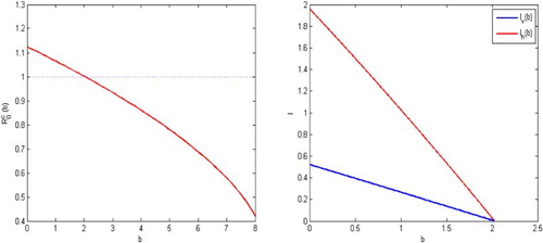If b<2.0252, the reproductive number $R_0^p\left(b\right)>1$ and there exists a stable endemic equilibrium, thus the disease spreads. It is shown in Figure 2.

Figure 2. The parameters given in Example 4.1, the threshold release are $\tilde{b}=2.0252$ and $b_c^p=8.2508$, respectively. For b>2.0252, the reproduction number of the system (1(1) $\begin{array}{rl}\frac{\mathrm{d}{S}_h}{\mathrm{d}t}& ={\mathrm{\Lambda }}_h-({\mu }_h+{\lambda }_h)S_h+{\theta }_h{R}_h,\\ \frac{\mathrm{d}{E}_h}{\mathrm{d}t}& ={\lambda }_h{S}_h-({\mu }_h+{\gamma }_h)E_h,\\ \frac{\mathrm{d}{I}_h}{\mathrm{d}t}& ={\gamma }_h{E}_h-({\mu }_h+{\delta }_h+{\eta }_h)I_h,\\ \frac{\mathrm{d}{R}_h}{\mathrm{d}t}& ={\eta }_h{I}_h-({\mu }_h+{\theta }_h)R_h,\end{array}$(1) ) and (12(12) $\begin{array}{rl}\frac{\mathrm{d}{N}_v}{\mathrm{d}t}& =\frac{{\alpha }_v{N}_v}{1+N_v+S_g}(1-{\xi }_v{N}_v)N_v-{\mu }_v{N}_v,\\ \frac{\mathrm{d}{E}_v}{\mathrm{d}t}& ={\lambda }_v(N_v-E_v-I_v)-({\mu }_v+{\gamma }_v)E_v,\\ \frac{\mathrm{d}{I}_v}{\mathrm{d}t}& ={\gamma }_v{E}_v-{\mu }_v{I}_v,\\ \frac{\mathrm{d}{S}_g}{\mathrm{d}t}& =B\left(N_v\right)-{\mu }_v{S}_g.\end{array}$(12) ) $R_0^p\left(b\right)<1$. For 0<b<2.0252, the reproduction number $R_0^p\left(b\right)>1$, as shown in the left figure. For the malaria model (1(1) $\begin{array}{rl}\frac{\mathrm{d}{S}_h}{\mathrm{d}t}& ={\mathrm{\Lambda }}_h-({\mu }_h+{\lambda }_h)S_h+{\theta }_h{R}_h,\\ \frac{\mathrm{d}{E}_h}{\mathrm{d}t}& ={\lambda }_h{S}_h-({\mu }_h+{\gamma }_h)E_h,\\ \frac{\mathrm{d}{I}_h}{\mathrm{d}t}& ={\gamma }_h{E}_h-({\mu }_h+{\delta }_h+{\eta }_h)I_h,\\ \frac{\mathrm{d}{R}_h}{\mathrm{d}t}& ={\eta }_h{I}_h-({\mu }_h+{\theta }_h)R_h,\end{array}$(1) ) and (12(12) $\begin{array}{rl}\frac{\mathrm{d}{N}_v}{\mathrm{d}t}& =\frac{{\alpha }_v{N}_v}{1+N_v+S_g}(1-{\xi }_v{N}_v)N_v-{\mu }_v{N}_v,\\ \frac{\mathrm{d}{E}_v}{\mathrm{d}t}& ={\lambda }_v(N_v-E_v-I_v)-({\mu }_v+{\gamma }_v)E_v,\\ \frac{\mathrm{d}{I}_v}{\mathrm{d}t}& ={\gamma }_v{E}_v-{\mu }_v{I}_v,\\ \frac{\mathrm{d}{S}_g}{\mathrm{d}t}& =B\left(N_v\right)-{\mu }_v{S}_g.\end{array}$(12) ), $I_h\left(b\right)$ and $I_v\left(b\right)$ decrease with the increasing of b as shown in the right figure. clearly, $I_h\left(b\right)$ and $I_v\left(b\right)$ all become negative for b>2.0252 which implies that no endemic equilibrium exists for $b\ge 2.0252$. Thus the disease dies out.

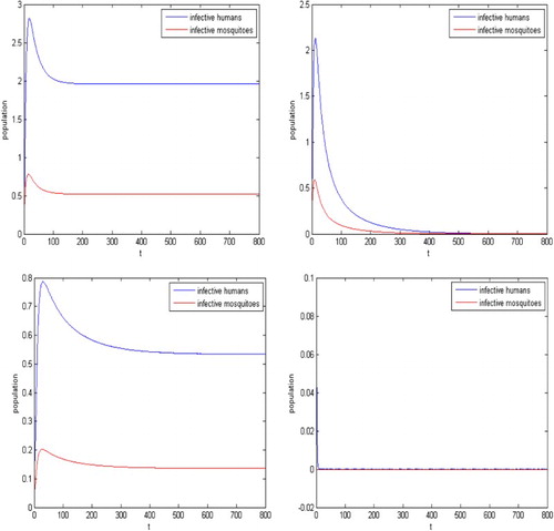
To show the transit dynamical impact of the releases of the sterile mosquitoes, we also present the solutions of the disease transmission system in Figure 3. When no sterile mosquitoes are released, the reproductive number $R_0\approx 1.1248>1$ and the disease spreads as shown on the upper left part in Figure 3. For the release rate $b=2.5>\tilde{b}$, the reproductive number is $R_0^p\approx 0.9683<1$. The infection dies out eventually, as is shown on the upper right part in Figure 3. For the release rate $b=1.5<\tilde{b}$, the reproductive number is $R_0^p\approx 1.0339>1$. Then solutions of the malaria model (1(1) $\begin{array}{rl}\frac{\mathrm{d}{S}_h}{\mathrm{d}t}& ={\mathrm{\Lambda }}_h-({\mu }_h+{\lambda }_h)S_h+{\theta }_h{R}_h,\\ \frac{\mathrm{d}{E}_h}{\mathrm{d}t}& ={\lambda }_h{S}_h-({\mu }_h+{\gamma }_h)E_h,\\ \frac{\mathrm{d}{I}_h}{\mathrm{d}t}& ={\gamma }_h{E}_h-({\mu }_h+{\delta }_h+{\eta }_h)I_h,\\ \frac{\mathrm{d}{R}_h}{\mathrm{d}t}& ={\eta }_h{I}_h-({\mu }_h+{\theta }_h)R_h,\end{array}$(1) ) and (12(12) $\begin{array}{rl}\frac{\mathrm{d}{N}_v}{\mathrm{d}t}& =\frac{{\alpha }_v{N}_v}{1+N_v+S_g}(1-{\xi }_v{N}_v)N_v-{\mu }_v{N}_v,\\ \frac{\mathrm{d}{E}_v}{\mathrm{d}t}& ={\lambda }_v(N_v-E_v-I_v)-({\mu }_v+{\gamma }_v)E_v,\\ \frac{\mathrm{d}{I}_v}{\mathrm{d}t}& ={\gamma }_v{E}_v-{\mu }_v{I}_v,\\ \frac{\mathrm{d}{S}_g}{\mathrm{d}t}& =B\left(N_v\right)-{\mu }_v{S}_g.\end{array}$(12) ) approach either the unique endemic equilibrium or the infection-free equilibrium associated with the trivial equilibrium of (13(13) $\begin{array}{rl}\frac{\mathrm{d}{N}_v}{\mathrm{d}t}& =\frac{{\alpha }_v{N}_v}{1+N_v+S_g}(1-{\xi }_v{N}_v)N_v-{\mu }_v{N}_v,\\ \frac{\mathrm{d}{S}_g}{\mathrm{d}t}& =b{N}_v-{\mu }_v{S}_g,\end{array}$(13) ) depending on the initial conditions, as shown in the lower left and right figures in Figure 3, respectively. Thus, the infection with the initial mosquitoes size close to $E_p^{+}$ spreads, the infection with the initial mosquitoes size close to $(0,0)$ can be eliminated eventually.

Figure 3. The parameters given in Example 4.1, the reproductive number for the malaria model (1(1) $\begin{array}{rl}\frac{\mathrm{d}{S}_h}{\mathrm{d}t}& ={\mathrm{\Lambda }}_h-({\mu }_h+{\lambda }_h)S_h+{\theta }_h{R}_h,\\ \frac{\mathrm{d}{E}_h}{\mathrm{d}t}& ={\lambda }_h{S}_h-({\mu }_h+{\gamma }_h)E_h,\\ \frac{\mathrm{d}{I}_h}{\mathrm{d}t}& ={\gamma }_h{E}_h-({\mu }_h+{\delta }_h+{\eta }_h)I_h,\\ \frac{\mathrm{d}{R}_h}{\mathrm{d}t}& ={\eta }_h{I}_h-({\mu }_h+{\theta }_h)R_h,\end{array}$(1) ) and (12(12) $\begin{array}{rl}\frac{\mathrm{d}{N}_v}{\mathrm{d}t}& =\frac{{\alpha }_v{N}_v}{1+N_v+S_g}(1-{\xi }_v{N}_v)N_v-{\mu }_v{N}_v,\\ \frac{\mathrm{d}{E}_v}{\mathrm{d}t}& ={\lambda }_v(N_v-E_v-I_v)-({\mu }_v+{\gamma }_v)E_v,\\ \frac{\mathrm{d}{I}_v}{\mathrm{d}t}& ={\gamma }_v{E}_v-{\mu }_v{I}_v,\\ \frac{\mathrm{d}{S}_g}{\mathrm{d}t}& =B\left(N_v\right)-{\mu }_v{S}_g.\end{array}$(12) ) is $R_0=1.1248>1$ and hence the infection spreads when there are no sterile mosquitoes released as shown in the upper left figure. With the sterile mosquitoes released, reproductive number is decreased. For $b=2.5>\tilde{b}=2.0252$, the reproduction number becomes $R_0^p\approx 0.9683$ and hence the infection dies out as shown in the upper right. For $b=1.5<\tilde{b}$, the reproductive number is $R_0^p\approx 1.0339>1$. Solutions for the malaria model (1(1) $\begin{array}{rl}\frac{\mathrm{d}{S}_h}{\mathrm{d}t}& ={\mathrm{\Lambda }}_h-({\mu }_h+{\lambda }_h)S_h+{\theta }_h{R}_h,\\ \frac{\mathrm{d}{E}_h}{\mathrm{d}t}& ={\lambda }_h{S}_h-({\mu }_h+{\gamma }_h)E_h,\\ \frac{\mathrm{d}{I}_h}{\mathrm{d}t}& ={\gamma }_h{E}_h-({\mu }_h+{\delta }_h+{\eta }_h)I_h,\\ \frac{\mathrm{d}{R}_h}{\mathrm{d}t}& ={\eta }_h{I}_h-({\mu }_h+{\theta }_h)R_h,\end{array}$(1) ) and (12(12) $\begin{array}{rl}\frac{\mathrm{d}{N}_v}{\mathrm{d}t}& =\frac{{\alpha }_v{N}_v}{1+N_v+S_g}(1-{\xi }_v{N}_v)N_v-{\mu }_v{N}_v,\\ \frac{\mathrm{d}{E}_v}{\mathrm{d}t}& ={\lambda }_v(N_v-E_v-I_v)-({\mu }_v+{\gamma }_v)E_v,\\ \frac{\mathrm{d}{I}_v}{\mathrm{d}t}& ={\gamma }_v{E}_v-{\mu }_v{I}_v,\\ \frac{\mathrm{d}{S}_g}{\mathrm{d}t}& =B\left(N_v\right)-{\mu }_v{S}_g.\end{array}$(12) ) approach either the unique endemic equilibrium or the equilibrium associated with the trivial equilibrium of (13(13) $\begin{array}{rl}\frac{\mathrm{d}{N}_v}{\mathrm{d}t}& =\frac{{\alpha }_v{N}_v}{1+N_v+S_g}(1-{\xi }_v{N}_v)N_v-{\mu }_v{N}_v,\\ \frac{\mathrm{d}{S}_g}{\mathrm{d}t}& =b{N}_v-{\mu }_v{S}_g,\end{array}$(13) ), depending on there initial values,as shown in the lower left and right figures.

Example 4.2

We use the following parameters for the malaria transmission: $\begin{array}{rl}{\alpha }_v& =100,{\mu }_v=0.2,{\xi }_v=0.0002,{\mathrm{\Lambda }}_h=15,\\ {\mu }_{h}7& =0.12,{\theta }_h=0.5,{\delta }_h=0.5,{\gamma }_h=0.6,{\eta }_h=0.7,\\ {\gamma }_v& =\mathrm{0.7.}r=2,{\beta }_h=0.01,{\beta }_v=\mathrm{0.8.}\end{array}$ By numerical calculations, we obtain $K_1=7.4259$, $K_2=1.7996$, $K_3=1.8189$, and $K_2+K_3<K_1$, $R_0^{\ast }\approx 0.8586$. Before the sterile mosquitoes are introduced, the reproductive number for the malaria model (1(1) $\begin{array}{rl}\frac{\mathrm{d}{S}_h}{\mathrm{d}t}& ={\mathrm{\Lambda }}_h-({\mu }_h+{\lambda }_h)S_h+{\theta }_h{R}_h,\\ \frac{\mathrm{d}{E}_h}{\mathrm{d}t}& ={\lambda }_h{S}_h-({\mu }_h+{\gamma }_h)E_h,\\ \frac{\mathrm{d}{I}_h}{\mathrm{d}t}& ={\gamma }_h{E}_h-({\mu }_h+{\delta }_h+{\eta }_h)I_h,\\ \frac{\mathrm{d}{R}_h}{\mathrm{d}t}& ={\eta }_h{I}_h-({\mu }_h+{\theta }_h)R_h,\end{array}$(1) ) and (12(12) $\begin{array}{rl}\frac{\mathrm{d}{N}_v}{\mathrm{d}t}& =\frac{{\alpha }_v{N}_v}{1+N_v+S_g}(1-{\xi }_v{N}_v)N_v-{\mu }_v{N}_v,\\ \frac{\mathrm{d}{E}_v}{\mathrm{d}t}& ={\lambda }_v(N_v-E_v-I_v)-({\mu }_v+{\gamma }_v)E_v,\\ \frac{\mathrm{d}{I}_v}{\mathrm{d}t}& ={\gamma }_v{E}_v-{\mu }_v{I}_v,\\ \frac{\mathrm{d}{S}_g}{\mathrm{d}t}& =B\left(N_v\right)-{\mu }_v{S}_g.\end{array}$(12) ) is $R_0\approx 0.9789>R_0^{\ast }$. Hence there exist two endemic equilibria $(14.1328,20.7359,2.8800,3.2741,4989.9,7.7474,27.1161)$ and $(114.6943,1.9275,0.2677,0.3022,4989.9,0.2528,0.8848)$, and the endemic equilibrium $(14.1328,20.7359,2.8800,3.2741,4989.9,7.7474,27.1161)$ is locally asymptotically stable. Hence, the disease may still spreads. It is shown in the left part in Figure 4. After the sterile mosquitoes are introduced, from (26(26) $b^{\ast }=:r_0-{\alpha }_v{\xi }_v{N}_v^{+}(\frac{R_0^{\ast }}{R_0}{)}^2-\frac{{\mu }_v}{N_v^{+}}{\left(\frac{R_0}{R_0^{\ast }}\right)}^2.$(26) ), we have $b^{\ast }=23.0311$. If b>23.031, the reproductive number of the system (1(1) $\begin{array}{rl}\frac{\mathrm{d}{S}_h}{\mathrm{d}t}& ={\mathrm{\Lambda }}_h-({\mu }_h+{\lambda }_h)S_h+{\theta }_h{R}_h,\\ \frac{\mathrm{d}{E}_h}{\mathrm{d}t}& ={\lambda }_h{S}_h-({\mu }_h+{\gamma }_h)E_h,\\ \frac{\mathrm{d}{I}_h}{\mathrm{d}t}& ={\gamma }_h{E}_h-({\mu }_h+{\delta }_h+{\eta }_h)I_h,\\ \frac{\mathrm{d}{R}_h}{\mathrm{d}t}& ={\eta }_h{I}_h-({\mu }_h+{\theta }_h)R_h,\end{array}$(1) ) and (12(12) $\begin{array}{rl}\frac{\mathrm{d}{N}_v}{\mathrm{d}t}& =\frac{{\alpha }_v{N}_v}{1+N_v+S_g}(1-{\xi }_v{N}_v)N_v-{\mu }_v{N}_v,\\ \frac{\mathrm{d}{E}_v}{\mathrm{d}t}& ={\lambda }_v(N_v-E_v-I_v)-({\mu }_v+{\gamma }_v)E_v,\\ \frac{\mathrm{d}{I}_v}{\mathrm{d}t}& ={\gamma }_v{E}_v-{\mu }_v{I}_v,\\ \frac{\mathrm{d}{S}_g}{\mathrm{d}t}& =B\left(N_v\right)-{\mu }_v{S}_g.\end{array}$(12) ) $R_0^p\left(b\right)<R_0^{\ast }$, then the disease dies out. For example, for the release rate $b=24.5>\tilde{b}$, the reproductive number is $R_0^p\approx 0.8502<R_0^{\ast }$. The infection dies out eventually, as shown in the right part in Figure 4.

Figure 4. The parameters given in Example 4.2, the reproductive number for the malaria model (1(1) $\begin{array}{rl}\frac{\mathrm{d}{S}_h}{\mathrm{d}t}& ={\mathrm{\Lambda }}_h-({\mu }_h+{\lambda }_h)S_h+{\theta }_h{R}_h,\\ \frac{\mathrm{d}{E}_h}{\mathrm{d}t}& ={\lambda }_h{S}_h-({\mu }_h+{\gamma }_h)E_h,\\ \frac{\mathrm{d}{I}_h}{\mathrm{d}t}& ={\gamma }_h{E}_h-({\mu }_h+{\delta }_h+{\eta }_h)I_h,\\ \frac{\mathrm{d}{R}_h}{\mathrm{d}t}& ={\eta }_h{I}_h-({\mu }_h+{\theta }_h)R_h,\end{array}$(1) ) and (12(12) $\begin{array}{rl}\frac{\mathrm{d}{N}_v}{\mathrm{d}t}& =\frac{{\alpha }_v{N}_v}{1+N_v+S_g}(1-{\xi }_v{N}_v)N_v-{\mu }_v{N}_v,\\ \frac{\mathrm{d}{E}_v}{\mathrm{d}t}& ={\lambda }_v(N_v-E_v-I_v)-({\mu }_v+{\gamma }_v)E_v,\\ \frac{\mathrm{d}{I}_v}{\mathrm{d}t}& ={\gamma }_v{E}_v-{\mu }_v{I}_v,\\ \frac{\mathrm{d}{S}_g}{\mathrm{d}t}& =B\left(N_v\right)-{\mu }_v{S}_g.\end{array}$(12) ) is $R_0\approx 0.9789>R_0^{\ast }$ and hence the infection may still spreads when there are no sterile mosquitoes released as shown in the left figure. With the sterile mosquitoes released, reproductive number is decreased. For $b=24.5>b^{\ast }=23.0311$, the reproduction number becomes $R_0^p\approx 0.8502<R_0^{\ast }$, backward bifurcation cannot occur for $R_0^p<1$ and hence the infection dies out as shown in the right figure.

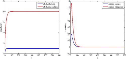
Example 4.3

We use, in this example, the same parameters as in Example 4.2 except $\mathrm{\Lambda }=13$. Before the sterile mosquitoes are introduced, the reproductive number for the malaria model (1(1) $\begin{array}{rl}\frac{\mathrm{d}{S}_h}{\mathrm{d}t}& ={\mathrm{\Lambda }}_h-({\mu }_h+{\lambda }_h)S_h+{\theta }_h{R}_h,\\ \frac{\mathrm{d}{E}_h}{\mathrm{d}t}& ={\lambda }_h{S}_h-({\mu }_h+{\gamma }_h)E_h,\\ \frac{\mathrm{d}{I}_h}{\mathrm{d}t}& ={\gamma }_h{E}_h-({\mu }_h+{\delta }_h+{\eta }_h)I_h,\\ \frac{\mathrm{d}{R}_h}{\mathrm{d}t}& ={\eta }_h{I}_h-({\mu }_h+{\theta }_h)R_h,\end{array}$(1) ) and (12(12) $\begin{array}{rl}\frac{\mathrm{d}{N}_v}{\mathrm{d}t}& =\frac{{\alpha }_v{N}_v}{1+N_v+S_g}(1-{\xi }_v{N}_v)N_v-{\mu }_v{N}_v,\\ \frac{\mathrm{d}{E}_v}{\mathrm{d}t}& ={\lambda }_v(N_v-E_v-I_v)-({\mu }_v+{\gamma }_v)E_v,\\ \frac{\mathrm{d}{I}_v}{\mathrm{d}t}& ={\gamma }_v{E}_v-{\mu }_v{I}_v,\\ \frac{\mathrm{d}{S}_g}{\mathrm{d}t}& =B\left(N_v\right)-{\mu }_v{S}_g.\end{array}$(12) ) is $R_0\approx 1.0515>1$ and hence the malaria transmission spreads. After the sterile mosquitoes are introduced, we have the existence threshold release value $b_c^p=99.67$ such that if b<99.67, system (13(13) $\begin{array}{rl}\frac{\mathrm{d}{N}_v}{\mathrm{d}t}& =\frac{{\alpha }_v{N}_v}{1+N_v+S_g}(1-{\xi }_v{N}_v)N_v-{\mu }_v{N}_v,\\ \frac{\mathrm{d}{S}_g}{\mathrm{d}t}& =b{N}_v-{\mu }_v{S}_g,\end{array}$(13) ) has two positive equilibria. If b>99.67, all wild mosquitoes are wiped out. However, the threshold release for the disease spread is $\tilde{b}=9.54$ and $b^{\ast }=33.2689$. If b<9.54, the reproductive number of the system (1(1) $\begin{array}{rl}\frac{\mathrm{d}{S}_h}{\mathrm{d}t}& ={\mathrm{\Lambda }}_h-({\mu }_h+{\lambda }_h)S_h+{\theta }_h{R}_h,\\ \frac{\mathrm{d}{E}_h}{\mathrm{d}t}& ={\lambda }_h{S}_h-({\mu }_h+{\gamma }_h)E_h,\\ \frac{\mathrm{d}{I}_h}{\mathrm{d}t}& ={\gamma }_h{E}_h-({\mu }_h+{\delta }_h+{\eta }_h)I_h,\\ \frac{\mathrm{d}{R}_h}{\mathrm{d}t}& ={\eta }_h{I}_h-({\mu }_h+{\theta }_h)R_h,\end{array}$(1) ) and (12(12) $\begin{array}{rl}\frac{\mathrm{d}{N}_v}{\mathrm{d}t}& =\frac{{\alpha }_v{N}_v}{1+N_v+S_g}(1-{\xi }_v{N}_v)N_v-{\mu }_v{N}_v,\\ \frac{\mathrm{d}{E}_v}{\mathrm{d}t}& ={\lambda }_v(N_v-E_v-I_v)-({\mu }_v+{\gamma }_v)E_v,\\ \frac{\mathrm{d}{I}_v}{\mathrm{d}t}& ={\gamma }_v{E}_v-{\mu }_v{I}_v,\\ \frac{\mathrm{d}{S}_g}{\mathrm{d}t}& =B\left(N_v\right)-{\mu }_v{S}_g.\end{array}$(12) ) $R_0^p\left(b\right)>1$ and thus the disease spreads. 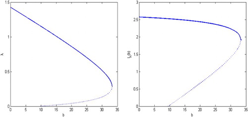If 9.54<b<33.2689, the reproductive number $R_0^{\ast }<R_0^p\left(b\right)<1$, there is two endemic equilibria, then an backward bifurcation can occur and the disease may still spreads. If b>33.2689, the reproductive number$R_0^p\left(b\right)<R_0^{\ast }<1$, the infection dies out eventually. The backward bifurcation diagrams of system (1(1) $\begin{array}{rl}\frac{\mathrm{d}{S}_h}{\mathrm{d}t}& ={\mathrm{\Lambda }}_h-({\mu }_h+{\lambda }_h)S_h+{\theta }_h{R}_h,\\ \frac{\mathrm{d}{E}_h}{\mathrm{d}t}& ={\lambda }_h{S}_h-({\mu }_h+{\gamma }_h)E_h,\\ \frac{\mathrm{d}{I}_h}{\mathrm{d}t}& ={\gamma }_h{E}_h-({\mu }_h+{\delta }_h+{\eta }_h)I_h,\\ \frac{\mathrm{d}{R}_h}{\mathrm{d}t}& ={\eta }_h{I}_h-({\mu }_h+{\theta }_h)R_h,\end{array}$(1) ) and (12(12) $\begin{array}{rl}\frac{\mathrm{d}{N}_v}{\mathrm{d}t}& =\frac{{\alpha }_v{N}_v}{1+N_v+S_g}(1-{\xi }_v{N}_v)N_v-{\mu }_v{N}_v,\\ \frac{\mathrm{d}{E}_v}{\mathrm{d}t}& ={\lambda }_v(N_v-E_v-I_v)-({\mu }_v+{\gamma }_v)E_v,\\ \frac{\mathrm{d}{I}_v}{\mathrm{d}t}& ={\gamma }_v{E}_v-{\mu }_v{I}_v,\\ \frac{\mathrm{d}{S}_g}{\mathrm{d}t}& =B\left(N_v\right)-{\mu }_v{S}_g.\end{array}$(12) ) for λ versus b and $I_h$ 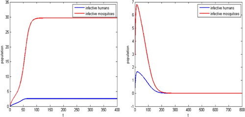versus b are shown in Figure 5. The dashed curve indicates the unstable equilibrium and the solid curve represents the stable equilibrium in all bifurcation diagrams. We also present the solutions of the disease transmission system in Figure 6. For example, for the release rate $\tilde{b}<b=20<b^{\ast }$, the reproductive number is $R_0^{\ast }<R_0^p\approx 0.9402<1$. The infection may still spreads, as is shown in the left figure in Figure 6. For the release rate $b=35>b^{\ast }$, the reproductive number is $R_0^p\approx 0.8472<R_0^{\ast }$. Thus the disease dies out, as is shown in the right side of Figure 6.

Figure 5. The backward bifurcation diagram of system (1(1) $\begin{array}{rl}\frac{\mathrm{d}{S}_h}{\mathrm{d}t}& ={\mathrm{\Lambda }}_h-({\mu }_h+{\lambda }_h)S_h+{\theta }_h{R}_h,\\ \frac{\mathrm{d}{E}_h}{\mathrm{d}t}& ={\lambda }_h{S}_h-({\mu }_h+{\gamma }_h)E_h,\\ \frac{\mathrm{d}{I}_h}{\mathrm{d}t}& ={\gamma }_h{E}_h-({\mu }_h+{\delta }_h+{\eta }_h)I_h,\\ \frac{\mathrm{d}{R}_h}{\mathrm{d}t}& ={\eta }_h{I}_h-({\mu }_h+{\theta }_h)R_h,\end{array}$(1) ) and (12(12) $\begin{array}{rl}\frac{\mathrm{d}{N}_v}{\mathrm{d}t}& =\frac{{\alpha }_v{N}_v}{1+N_v+S_g}(1-{\xi }_v{N}_v)N_v-{\mu }_v{N}_v,\\ \frac{\mathrm{d}{E}_v}{\mathrm{d}t}& ={\lambda }_v(N_v-E_v-I_v)-({\mu }_v+{\gamma }_v)E_v,\\ \frac{\mathrm{d}{I}_v}{\mathrm{d}t}& ={\gamma }_v{E}_v-{\mu }_v{I}_v,\\ \frac{\mathrm{d}{S}_g}{\mathrm{d}t}& =B\left(N_v\right)-{\mu }_v{S}_g.\end{array}$(12) ) for λ versus b as shown in the left figure. The backward bifurcation diagram of system (1(1) $\begin{array}{rl}\frac{\mathrm{d}{S}_h}{\mathrm{d}t}& ={\mathrm{\Lambda }}_h-({\mu }_h+{\lambda }_h)S_h+{\theta }_h{R}_h,\\ \frac{\mathrm{d}{E}_h}{\mathrm{d}t}& ={\lambda }_h{S}_h-({\mu }_h+{\gamma }_h)E_h,\\ \frac{\mathrm{d}{I}_h}{\mathrm{d}t}& ={\gamma }_h{E}_h-({\mu }_h+{\delta }_h+{\eta }_h)I_h,\\ \frac{\mathrm{d}{R}_h}{\mathrm{d}t}& ={\eta }_h{I}_h-({\mu }_h+{\theta }_h)R_h,\end{array}$(1) ) and (12(12) $\begin{array}{rl}\frac{\mathrm{d}{N}_v}{\mathrm{d}t}& =\frac{{\alpha }_v{N}_v}{1+N_v+S_g}(1-{\xi }_v{N}_v)N_v-{\mu }_v{N}_v,\\ \frac{\mathrm{d}{E}_v}{\mathrm{d}t}& ={\lambda }_v(N_v-E_v-I_v)-({\mu }_v+{\gamma }_v)E_v,\\ \frac{\mathrm{d}{I}_v}{\mathrm{d}t}& ={\gamma }_v{E}_v-{\mu }_v{I}_v,\\ \frac{\mathrm{d}{S}_g}{\mathrm{d}t}& =B\left(N_v\right)-{\mu }_v{S}_g.\end{array}$(12) ) for $I_h$ versus b as shown in the right figure.

5. Concluding remarks

In this paper, we focus on the study of the impact of proportionally releasing sterile mosquitoes on malaria transmission. We first formulated a simple compartmental SEIR model for malaria transmission in Section 2. This is our baseline model to be used for incorporating sterile mosquitoes into the malaria transmission. In our system, the mating rate is assumed to be a saturated function. We derived the formula of the reproductive number of baseline model and showed the existence of an endemic equilibrium, as the reproductive number is greater than one. We also discussed the backward bifurcation for the baseline model when $R_0<1$.

Figure 6. With the parameters given in Example 4.3, the threshold values are $\tilde{b}=9.54$ and $b^{\ast }=33.2689$. for $\tilde{b}<b=20<b^{\ast }$, the reproduction number becomes $R_0^{\ast }<R_0^p\approx 0.9402<1$, backward bifurcation can occur and hence the disease may still spreads as shown in the left figure. For $b=35>b^{\ast }$, the reproductive number is $R_0^p\approx 0.8472<R_0^{\ast }$. Thus the disease dies out as shown in the right figure.

We then introduced the sterile mosquitoes into the baseline model in Section 3. We considered the case that the number of releases is proportional to the population size of the wild mosquitoes and derive formulas of the reproductive number $R_0^p$ and sub-threshold $R_0^{\ast }$ of models with sterile mosquitoes. We analyse three releasing thresholds $b_c^p$, $\tilde{b}$ and $b^{\ast }$ and demonstrate their effect in Theorem 3.3. It is clear that $\tilde{b}<b^{\ast }<b_c^p$. If the releasing rate b satisfies $b>b_c^p$, then the wild mosquitoes are wiped out and there will be no infection; If $b^{\ast }<b<b_c^p$, the sterile and wild mosquitoes coexist, but the reproductive number $R_0^p<R_0^{\ast }<1$, thus the disease will eventually go extinct; If $\tilde{b}<b<b^{\ast }$, the sterile and wild mosquitoes coexist, while the reproductive number $R_0^{\ast }<R_0^p<1$, thus malaria may still persist; If $b<\tilde{b}$, then $R_0^p>1$, and the disease will spread.

The impact of releasing sterile mosquitoes is studied through theoretical analysis and numerical simulation in Section 4. After the sterile mosquitoes are introduced, the reproductive number is smaller than that for the model without sterile mosquitoes. It implies that the malaria transmission can be controlled more easily by releasing the sterile mosquitoes. From [12], if the release rate b is big enough (such as $b>b_c^p$), all wild mosquitoes are eventually wiped out, which leads to the infection dies out eventually. This case may be only ideal but not be feasible in practice. A more realistic situation is that we only need to release enough sterile mosquitoes (such as $b^{\ast }<b<b_c^p$), such that the reproductive number of the malaria transmission is brought to below one or $R_0^{\ast }$, then the infection dies out eventually. If the releasing rate is too small(such as $b<b^{\ast }$), then the disease cannot be eliminated. From the above analyse we know that the best interval for releasing rate b is $b^{\ast }<b<b_c^p$. However, even if the reproductive number is still above one, the ultimate infective components for both humans and mosquitoes decrease with the increasing of the release rate b.

While we provided investigations of the impact of releasing sterile mosquitoes on malaria transmission, such investigations are only preliminary. The interactive dynamics of wild and sterile mosquitoes are so complex that investigations of effects on malaria transmission can be challenging. The release rate in this paper has been assumed to be proportional to the population size of the wild mosquitoes. When the wild mosquitoes population size is small, the proportional release rate seems economically optimal, but not necessary when the wild mosquitoes population size is big since the number of releases is supposed to be big as well. Then we can consider a new strategy such that the release rate is proportional to the wild mosquitoes population size when the wild mosquitoes population size is small, but is saturated and approaches a constant when the wild mosquitoes population size is sufficiently large. That is, the release rate can take the form of $B\left(N_v\right)=\left(b{N}_v\right)/\left(1+N_v\right)$, which is a Holling-II type function. Moreover, in this paper the mosquito population has been assumed to be homogenous. Malaria model with stage-structured wild and sterile mosquitoes are needed to gain further insight into the impact for malaria transmission. We leave these tasks for future consideration.

Disclosure statement

No potential conflict of interest was reported by the authors.

Additional information

Funding

This Research was partially supported by the National Nature Science Foundation of China [No.11371161, 11471133], the Fundamental Research Funds for the Central Universities, Central China Normal University [No.CCNU15A02055] and the Fundamental Research Funds for the Central Universities, South-Central University for Nationalities [No.CZQ13016].

Appendix

A.1. The reproductive number

By investigating the local stability of the infection-free equilibrium, we can calculate the reproductive number of system (1(1) $\begin{array}{rl}\frac{\mathrm{d}{S}_h}{\mathrm{d}t}& ={\mathrm{\Lambda }}_h-({\mu }_h+{\lambda }_h)S_h+{\theta }_h{R}_h,\\ \frac{\mathrm{d}{E}_h}{\mathrm{d}t}& ={\lambda }_h{S}_h-({\mu }_h+{\gamma }_h)E_h,\\ \frac{\mathrm{d}{I}_h}{\mathrm{d}t}& ={\gamma }_h{E}_h-({\mu }_h+{\delta }_h+{\eta }_h)I_h,\\ \frac{\mathrm{d}{R}_h}{\mathrm{d}t}& ={\eta }_h{I}_h-({\mu }_h+{\theta }_h)R_h,\end{array}$(1) ) and (8(8) $\begin{array}{rl}\frac{\mathrm{d}{N}_v}{\mathrm{d}t}& =\frac{{\alpha }_v{N}_v}{1+N_v}(1-{\xi }_v{N}_v)N_v-{\mu }_v{N}_v,\\ \frac{\mathrm{d}{E}_v}{\mathrm{d}t}& ={\lambda }_v(N_v-E_v-I_v)-({\mu }_v+{\gamma }_v)E_v,\\ \frac{\mathrm{d}{I}_v}{\mathrm{d}t}& ={\gamma }_v{E}_v-{\mu }_v{I}_v.\end{array}$(8) ) as follows. The Jacobian matrix at the infection-free equilibrium $(S_h,R_h,I_h,E_h,I_v,E_v,N_v)=(N_h^0,0,0,0,0,0,N_v^{+})$ has the form $\left(\begin{array}{ccc}{J}_{21}& \cdot & 0\\ 0& J_{22}& 0\\ 0& \cdot & J_{23}\end{array}\right),$ where $\begin{array}{rl}{J}_{21}& :=\left(\begin{array}{cc}-{\mu }_h& {\theta }_h\\ 0& -{\sigma }_3\end{array}\right),\\ J_{22}& :=\left(\begin{array}{cccc}-{\sigma }_2& {\gamma }_h& 0& 0\\ 0& -{\sigma }_1& r{\beta }_v& 0\\ 0& 0& -{\mu }_v& {\gamma }_v\\ r{\beta }_h{N}_v^{+}/N_h^0& 0& 0& -{\sigma }_v\end{array}\right),\\ J_{23}& =\frac{{\alpha }_v(1-{\xi }_v{N}_v^{+})}{(1+N_v^{+}{)}^2}-\frac{{\alpha }_v{\xi }_v{N}_v^{+}}{1+N_v^{+}},\end{array}$ and we write ${\sigma }_1:={\mu }_h+{\gamma }_h$, ${\sigma }_2:={\mu }_h+{\delta }_h+{\eta }_h$, ${\sigma }_3:={\mu }_h+{\theta }_h$, ${\sigma }_v:={\mu }_v+{\gamma }_v$. We know that $J_{23}<0$ from [12], and hence the local stability of the infection-free equilibrium is determined by matrix $J_{22}$.

It follows from the M-matrix theory [5,8] that all eigenvalues of $J_{22}$ have negative real part, that is, the infection-free equilibrium is locally asymptotically stable, if the determinant $det{J}_{22}={\sigma }_1{\sigma }_2{\mu }_v{\sigma }_v-r^2{\gamma }_h{\gamma }_v{\beta }_v{\beta }_h{N}_v^{+}/N_h^0={\sigma }_1{\sigma }_2{\sigma }_v{\mu }_v(1-\frac{r^2{\beta }_h{\beta }_v{\gamma }_h{\gamma }_v{N}_v^{+}}{{\sigma }_1{\sigma }_2{\sigma }_v{\mu }_v{N}_h^0})$ is positive.

Then we can define the reproductive number of infection for system (1(1) $\begin{array}{rl}\frac{\mathrm{d}{S}_h}{\mathrm{d}t}& ={\mathrm{\Lambda }}_h-({\mu }_h+{\lambda }_h)S_h+{\theta }_h{R}_h,\\ \frac{\mathrm{d}{E}_h}{\mathrm{d}t}& ={\lambda }_h{S}_h-({\mu }_h+{\gamma }_h)E_h,\\ \frac{\mathrm{d}{I}_h}{\mathrm{d}t}& ={\gamma }_h{E}_h-({\mu }_h+{\delta }_h+{\eta }_h)I_h,\\ \frac{\mathrm{d}{R}_h}{\mathrm{d}t}& ={\eta }_h{I}_h-({\mu }_h+{\theta }_h)R_h,\end{array}$(1) ) and (8(8) $\begin{array}{rl}\frac{\mathrm{d}{N}_v}{\mathrm{d}t}& =\frac{{\alpha }_v{N}_v}{1+N_v}(1-{\xi }_v{N}_v)N_v-{\mu }_v{N}_v,\\ \frac{\mathrm{d}{E}_v}{\mathrm{d}t}& ={\lambda }_v(N_v-E_v-I_v)-({\mu }_v+{\gamma }_v)E_v,\\ \frac{\mathrm{d}{I}_v}{\mathrm{d}t}& ={\gamma }_v{E}_v-{\mu }_v{I}_v.\end{array}$(8) ) as (9(9) $R_0:=\sqrt{\frac{r^2{\beta }_h{\beta }_v{\gamma }_h{\gamma }_v{N}_v^{+}}{({\mu }_h+{\gamma }_h)({\mu }_h+{\delta }_h+{\eta }_h)({\mu }_v+{\gamma }_v){\mu }_v{N}_h^0}}.$(9) ), and the infection-free equilibrium $(N_h^0,0,0,0,0,0,N_v^{+})$ is locally asymptotically stable if $R_0<1$ and unstable if $R_0>1$.

A.2. Endemic equilibrium

We can solve the components for the humans at an endemic equilibrium, in terms of ${\lambda }_h$, as (A1) $\begin{array}{rl}{S}_h& =\frac{{\mathrm{\Lambda }}_h}{{\mu }_h(1+K_1{\lambda }_h)},E_h=\frac{{\mathrm{\Lambda }}_h{\lambda }_h}{{\mu }_h{\sigma }_1(1+K_1{\lambda }_h)},\\ I_h& =\frac{{\mathrm{\Lambda }}_h{\lambda }_h{\gamma }_h}{{\mu }_h{\sigma }_1{\sigma }_2(1+K_1{\lambda }_h)},R_h=\frac{{\mathrm{\Lambda }}_h{\lambda }_h{\gamma }_h{\eta }_h}{{\mu }_h{\sigma }_1{\sigma }_2{\sigma }_3(1+K_1{\lambda }_h)},\end{array}$(A1) where $K_1:=1/\left({\mu }_h\right)-{\theta }_h\left({\eta }_h{\gamma }_h\right)/\left({\mu }_h{\sigma }_1{\sigma }_2{\sigma }_3\right)>0$. We further write $K_2:=\left({\sigma }_2{\sigma }_3+{\sigma }_3{\gamma }_h+{\gamma }_h{\eta }_h\right)/\left({\sigma }_1{\sigma }_2{\sigma }_3\right)$ and have (A2) $N_h=\frac{{\mathrm{\Lambda }}_h(1+K_2{\lambda }_h)}{{\mu }_h(1+K_1{\lambda }_h)}.$(A2)

Substituting $I_h$ in (A1(A1) $\begin{array}{rl}{S}_h& =\frac{{\mathrm{\Lambda }}_h}{{\mu }_h(1+K_1{\lambda }_h)},E_h=\frac{{\mathrm{\Lambda }}_h{\lambda }_h}{{\mu }_h{\sigma }_1(1+K_1{\lambda }_h)},\\ I_h& =\frac{{\mathrm{\Lambda }}_h{\lambda }_h{\gamma }_h}{{\mu }_h{\sigma }_1{\sigma }_2(1+K_1{\lambda }_h)},R_h=\frac{{\mathrm{\Lambda }}_h{\lambda }_h{\gamma }_h{\eta }_h}{{\mu }_h{\sigma }_1{\sigma }_2{\sigma }_3(1+K_1{\lambda }_h)},\end{array}$(A1) ) and $N_h$ in (A2(A2) $N_h=\frac{{\mathrm{\Lambda }}_h(1+K_2{\lambda }_h)}{{\mu }_h(1+K_1{\lambda }_h)}.$(A2) ) into (3(3) ${\lambda }_v=r{\beta }_h\frac{I_h}{N_h},$(3) ), we get (A3) ${\lambda }_v=B_1\frac{{\lambda }_h}{1+K_2{\lambda }_h},$(A3) where $B_1:=\left(r{\beta }_h{\gamma }_h\right)/\left({\sigma }_1{\sigma }_2\right)$.

We then solve the components for the mosquitoes and have $\begin{array}{rl}{E}_v& =\frac{{\lambda }_v}{{\sigma }_v}{S}_v,\\ I_v& =\frac{{\gamma }_v{\lambda }_v}{{\mu }_v{\sigma }_v}{S}_v.\end{array}$ Since (A4) $N_v=S_v+E_v+I_v=(1+\frac{{\lambda }_v}{{\sigma }_v}+\frac{{\gamma }_v{\lambda }_v}{{\mu }_v{\sigma }_v})S_v=\frac{{\mu }_v+{\lambda }_v}{{\mu }_v}{S}_v,$(A4) then $S_v=\frac{{\mu }_v}{{\mu }_v+{\lambda }_v}{N}_v,$ which leads to (A5) $I_v=\frac{{\gamma }_v{\lambda }_v}{{\sigma }_v({\mu }_v+{\lambda }_v)}{N}_v=\frac{{\gamma }_v{B}_1{\lambda }_h{N}_v}{{\sigma }_v({\mu }_v+(B_1+{\mu }_v{K}_2\left){\lambda }_h\right)}.$(A5)

Then, substituting (A5(A5) $I_v=\frac{{\gamma }_v{\lambda }_v}{{\sigma }_v({\mu }_v+{\lambda }_v)}{N}_v=\frac{{\gamma }_v{B}_1{\lambda }_h{N}_v}{{\sigma }_v({\mu }_v+(B_1+{\mu }_v{K}_2\left){\lambda }_h\right)}.$(A5) ) into (4(4) ${\lambda }_h={\beta }_{v}r\frac{N_v}{N_h}\frac{I_v}{N_v}=r{\beta }_v\frac{I_v}{N_h},$(4) ) yields (A6) ${\lambda }_h=\frac{r{\beta }_v}{N_h}{I}_v=\frac{r{\beta }_v{\mu }_h(1+K_1{\lambda }_h)}{{\mathrm{\Lambda }}_h(1+K_2{\lambda }_h)}\frac{{\gamma }_v{B}_1{\lambda }_h{N}_v}{{\sigma }_v({\mu }_v+(B_1+{\mu }_v{K}_2\left){\lambda }_h\right)},$(A6) which leads to $\begin{array}{rl}1& =\frac{r{\beta }_v{\mu }_h(1+K_1{\lambda }_h)}{{\mathrm{\Lambda }}_h(1+K_2{\lambda }_h)}\frac{{\mu }_v{\gamma }_v{B}_1{N}_v}{{\sigma }_v({\mu }_v+(B_1+{\mu }_v{K}_2\left){\lambda }_h\right){\mu }_v}\\ & =\frac{r^2{\beta }_v{\beta }_h{\mu }_h{\gamma }_v{\gamma }_h{\mu }_v(1+K_1{\lambda }_h)N_v}{{\mathrm{\Lambda }}_h{\sigma }_1{\sigma }_2{\sigma }_v{\mu }_v(1+K_2{\lambda }_h)({\mu }_v+(B_1+{\mu }_v{K}_2\left){\lambda }_h\right)}\\ & =R_0^2\frac{N_v}{N_v^{+}}\frac{{\mu }_v(1+K_1{\lambda }_h)}{(1+K_2{\lambda }_h)({\mu }_v+(B_1+{\mu }_v{K}_2\left){\lambda }_h\right)}.\end{array}$ We write ${\lambda }_h=\lambda$ and define (A7) $G_1(\lambda ,N_v):=K_2(B_1+{\mu }_v{K}_2){\lambda }^2+(B_1+{\mu }_v(2K_2-R_0^2{K}_1\frac{N_v}{N_v^{+}}))\lambda +(1-R_0^2\frac{N_v}{N_v^{+}}){\mu }_v.$(A7) Then the endemic equilibria of system (1(1) $\begin{array}{rl}\frac{\mathrm{d}{S}_h}{\mathrm{d}t}& ={\mathrm{\Lambda }}_h-({\mu }_h+{\lambda }_h)S_h+{\theta }_h{R}_h,\\ \frac{\mathrm{d}{E}_h}{\mathrm{d}t}& ={\lambda }_h{S}_h-({\mu }_h+{\gamma }_h)E_h,\\ \frac{\mathrm{d}{I}_h}{\mathrm{d}t}& ={\gamma }_h{E}_h-({\mu }_h+{\delta }_h+{\eta }_h)I_h,\\ \frac{\mathrm{d}{R}_h}{\mathrm{d}t}& ={\eta }_h{I}_h-({\mu }_h+{\theta }_h)R_h,\end{array}$(1) ) and (8(8) $\begin{array}{rl}\frac{\mathrm{d}{N}_v}{\mathrm{d}t}& =\frac{{\alpha }_v{N}_v}{1+N_v}(1-{\xi }_v{N}_v)N_v-{\mu }_v{N}_v,\\ \frac{\mathrm{d}{E}_v}{\mathrm{d}t}& ={\lambda }_v(N_v-E_v-I_v)-({\mu }_v+{\gamma }_v)E_v,\\ \frac{\mathrm{d}{I}_v}{\mathrm{d}t}& ={\gamma }_v{E}_v-{\mu }_v{I}_v.\end{array}$(8) ) correspond to the positive roots of $G_1(\lambda ,N_v)=0$.

For $N_v=N_v^{+}$, (A7(A7) $G_1(\lambda ,N_v):=K_2(B_1+{\mu }_v{K}_2){\lambda }^2+(B_1+{\mu }_v(2K_2-R_0^2{K}_1\frac{N_v}{N_v^{+}}))\lambda +(1-R_0^2\frac{N_v}{N_v^{+}}){\mu }_v.$(A7) ) becomes (A8) $G_1(\lambda ,N_v^{+}):=K_2(B_1+{\mu }_v{K}_2){\lambda }^2+(B_1+{\mu }_v(2K_2-R_0^2{K}_1))\lambda +(1-R_0^2){\mu }_v.$(A8) Clearly, equation $G_1(\lambda ,N_v^{+})=0$ has unique positive root and hence system (1(1) $\begin{array}{rl}\frac{\mathrm{d}{S}_h}{\mathrm{d}t}& ={\mathrm{\Lambda }}_h-({\mu }_h+{\lambda }_h)S_h+{\theta }_h{R}_h,\\ \frac{\mathrm{d}{E}_h}{\mathrm{d}t}& ={\lambda }_h{S}_h-({\mu }_h+{\gamma }_h)E_h,\\ \frac{\mathrm{d}{I}_h}{\mathrm{d}t}& ={\gamma }_h{E}_h-({\mu }_h+{\delta }_h+{\eta }_h)I_h,\\ \frac{\mathrm{d}{R}_h}{\mathrm{d}t}& ={\eta }_h{I}_h-({\mu }_h+{\theta }_h)R_h,\end{array}$(1) ) and (8(8) $\begin{array}{rl}\frac{\mathrm{d}{N}_v}{\mathrm{d}t}& =\frac{{\alpha }_v{N}_v}{1+N_v}(1-{\xi }_v{N}_v)N_v-{\mu }_v{N}_v,\\ \frac{\mathrm{d}{E}_v}{\mathrm{d}t}& ={\lambda }_v(N_v-E_v-I_v)-({\mu }_v+{\gamma }_v)E_v,\\ \frac{\mathrm{d}{I}_v}{\mathrm{d}t}& ={\gamma }_v{E}_v-{\mu }_v{I}_v.\end{array}$(8) ) has an endemic equilibrium if $R_0>1$.

A.3. Backward bifurcation

We show that system (1(1) $\begin{array}{rl}\frac{\mathrm{d}{S}_h}{\mathrm{d}t}& ={\mathrm{\Lambda }}_h-({\mu }_h+{\lambda }_h)S_h+{\theta }_h{R}_h,\\ \frac{\mathrm{d}{E}_h}{\mathrm{d}t}& ={\lambda }_h{S}_h-({\mu }_h+{\gamma }_h)E_h,\\ \frac{\mathrm{d}{I}_h}{\mathrm{d}t}& ={\gamma }_h{E}_h-({\mu }_h+{\delta }_h+{\eta }_h)I_h,\\ \frac{\mathrm{d}{R}_h}{\mathrm{d}t}& ={\eta }_h{I}_h-({\mu }_h+{\theta }_h)R_h,\end{array}$(1) ) and (8(8) $\begin{array}{rl}\frac{\mathrm{d}{N}_v}{\mathrm{d}t}& =\frac{{\alpha }_v{N}_v}{1+N_v}(1-{\xi }_v{N}_v)N_v-{\mu }_v{N}_v,\\ \frac{\mathrm{d}{E}_v}{\mathrm{d}t}& ={\lambda }_v(N_v-E_v-I_v)-({\mu }_v+{\gamma }_v)E_v,\\ \frac{\mathrm{d}{I}_v}{\mathrm{d}t}& ={\gamma }_v{E}_v-{\mu }_v{I}_v.\end{array}$(8) ) undergo backward bifurcation.

An endemic equilibrium of system (1(1) $\begin{array}{rl}\frac{\mathrm{d}{S}_h}{\mathrm{d}t}& ={\mathrm{\Lambda }}_h-({\mu }_h+{\lambda }_h)S_h+{\theta }_h{R}_h,\\ \frac{\mathrm{d}{E}_h}{\mathrm{d}t}& ={\lambda }_h{S}_h-({\mu }_h+{\gamma }_h)E_h,\\ \frac{\mathrm{d}{I}_h}{\mathrm{d}t}& ={\gamma }_h{E}_h-({\mu }_h+{\delta }_h+{\eta }_h)I_h,\\ \frac{\mathrm{d}{R}_h}{\mathrm{d}t}& ={\eta }_h{I}_h-({\mu }_h+{\theta }_h)R_h,\end{array}$(1) ) and (8(8) $\begin{array}{rl}\frac{\mathrm{d}{N}_v}{\mathrm{d}t}& =\frac{{\alpha }_v{N}_v}{1+N_v}(1-{\xi }_v{N}_v)N_v-{\mu }_v{N}_v,\\ \frac{\mathrm{d}{E}_v}{\mathrm{d}t}& ={\lambda }_v(N_v-E_v-I_v)-({\mu }_v+{\gamma }_v)E_v,\\ \frac{\mathrm{d}{I}_v}{\mathrm{d}t}& ={\gamma }_v{E}_v-{\mu }_v{I}_v.\end{array}$(8) ) corresponds a positive root of the equation $G_1(\lambda ,N_v^{+})=0$, that is (A9) $K_2(B_1+{\mu }_v{K}_2){\lambda }^2+(B_1+{\mu }_v(2K_2-R_0^2{K}_1))\lambda +(1-R_0^2){\mu }_v=0,$(A9) or $K_2(\frac{B_1}{{\mu }_v}+K_2){\lambda }^2+(\frac{B_1}{{\mu }_v}+(2K_2-R_0^2{K}_1))\lambda +(1-R_0^2)=0.$ Let $K_3=K_2+\left(B_1/{\mu }_v\right)$, then (A9(A9) $K_2(B_1+{\mu }_v{K}_2){\lambda }^2+(B_1+{\mu }_v(2K_2-R_0^2{K}_1))\lambda +(1-R_0^2){\mu }_v=0,$(A9) ) turns into (A10) $K_2{K}_3{\lambda }^2+(K_3+K_2-R_0^2{K}_1)\lambda +(1-R_0^2)=0,$(A10) If $R_0>1$, there exists a unique positive root of (A10(A10) $K_2{K}_3{\lambda }^2+(K_3+K_2-R_0^2{K}_1)\lambda +(1-R_0^2)=0,$(A10) ). If $R_0=1$, then when $K_2+K_3<K_1$, Equation (A10(A10) $K_2{K}_3{\lambda }^2+(K_3+K_2-R_0^2{K}_1)\lambda +(1-R_0^2)=0,$(A10) ) has a unique positive root $\lambda =\frac{K_1-(K_2+K_3)}{K_2{K}_4}.$

For $R_0\le 1$, if $K_2+K_3\ge K_1$, then Equation (A10(A10) $K_2{K}_3{\lambda }^2+(K_3+K_2-R_0^2{K}_1)\lambda +(1-R_0^2)=0,$(A10) ) has no positive root and thus there is no backward bifurcation.

Now we assume$R_0<1$ and $K_2+K_3<K_1$. Clearly, if $R_0<\sqrt{\left(\right(K_2+K_3\left)/K_1\right)}<1$, there exists no positive root of (A10(A10) $K_2{K}_3{\lambda }^2+(K_3+K_2-R_0^2{K}_1)\lambda +(1-R_0^2)=0,$(A10) ). If $\sqrt{\left(\right(K_2+K_3\left)/K_1\right)}\le R_0<1$, we write $R_0^2=c$ for convenience, then Equation (A10(A10) $K_2{K}_3{\lambda }^2+(K_3+K_2-R_0^2{K}_1)\lambda +(1-R_0^2)=0,$(A10) ) becomes $K_2{K}_3{\lambda }^2+(K_3+K_2-c{K}_1)\lambda +(1-c)=0.$

Let $\begin{array}{rl}\mathrm{\Delta }& :=(K_2+K_3-c{K}_1{)}^2-4K_2{K}_3(1-c)\\ & =K_1^2{c}^2+[4K_2{K}_3-2K_3(K_2+K_3\left)\right]c+(K_2-K_3{)}^2,\end{array}$ then the roots of Equation (A10(A10) $K_2{K}_3{\lambda }^2+(K_3+K_2-R_0^2{K}_1)\lambda +(1-R_0^2)=0,$(A10) ) are given by (A11) $\lambda =\frac{c{K}_1-K_2-K_3\pm \sqrt{(c{K}_1-K_2-K_3{)}^2-4K_2{K}_1(1-c)}}{2K_2{K}_3}.$(A11) Equation (A10(A10) $K_2{K}_3{\lambda }^2+(K_3+K_2-R_0^2{K}_1)\lambda +(1-R_0^2)=0,$(A10) ) has two positive roots if $\mathrm{\Delta }>0$, a unique positive root if $\mathrm{\Delta }=0$, and no positive root if $\mathrm{\Delta }<0$.

From $c>\left(\right(K_2+K_3\left)/K_1\right)$ and $\mathrm{\Delta }>0$, it follows that $c>\frac{K_1(K_2+K_3)-2K_2{K}_3+2\sqrt{K_2{K}_3(K_2-K_1)(K_3-K_1)}}{K_1^2}.$ From $c>\left(\right(K_2+K_3\left)/K_1\right)$ and $\mathrm{\Delta }=0$, it follows that $c=\frac{K_1(K_2+K_3)-2K_2{K}_3+2\sqrt{K_2{K}_3(K_2-K_1)(K_3-K_1)}}{K_1^2}.$ From $c>\left(\right(K_2+K_3\left)/K_1\right)$ and $\mathrm{\Delta }<0$, it follows that $\frac{K_2+K_3}{K_1}<c<\frac{K_1(K_2+K_3)-2K_2{K}_3+2\sqrt{K_2{K}_3(K_2-K_1)(K_3-K_3)}}{K_1^2}.$ We write $R_0^{\ast }$ as (10(10) $R_0^{\ast }:=\frac{{\left(K_1\right(K_2+K_3)-2K_2{K}_3+2\sqrt{K_2{K}_3(K_2-K_1)(K_3-K_1)})}^{1/2}}{K_1},$(10) ), then the results about endemic equilibria of (1(1) $\begin{array}{rl}\frac{\mathrm{d}{S}_h}{\mathrm{d}t}& ={\mathrm{\Lambda }}_h-({\mu }_h+{\lambda }_h)S_h+{\theta }_h{R}_h,\\ \frac{\mathrm{d}{E}_h}{\mathrm{d}t}& ={\lambda }_h{S}_h-({\mu }_h+{\gamma }_h)E_h,\\ \frac{\mathrm{d}{I}_h}{\mathrm{d}t}& ={\gamma }_h{E}_h-({\mu }_h+{\delta }_h+{\eta }_h)I_h,\\ \frac{\mathrm{d}{R}_h}{\mathrm{d}t}& ={\eta }_h{I}_h-({\mu }_h+{\theta }_h)R_h,\end{array}$(1) ) and (8(8) $\begin{array}{rl}\frac{\mathrm{d}{N}_v}{\mathrm{d}t}& =\frac{{\alpha }_v{N}_v}{1+N_v}(1-{\xi }_v{N}_v)N_v-{\mu }_v{N}_v,\\ \frac{\mathrm{d}{E}_v}{\mathrm{d}t}& ={\lambda }_v(N_v-E_v-I_v)-({\mu }_v+{\gamma }_v)E_v,\\ \frac{\mathrm{d}{I}_v}{\mathrm{d}t}& ={\gamma }_v{E}_v-{\mu }_v{I}_v.\end{array}$(8) ) can be summarized in Theorem 2.1.

References

- L. Alphey, M. Benedict, R. Bellini, G.G. Clark, D.A. Dame, M.W. Service, and S.L. Dobson, Sterile-insect methods for control of mosquito-borne diseases: An analysis. Vector-Borne Zoonotic Dis. 10 (2010), pp. 295–311 doi: 10.1089/vbz.2009.0014
- L. Alphey, M. Benedict, R. Bellini, G.G. Clark, D.A. Dame, M.W. Service, and S.L. Dobson, Infectious Diseases of Humans, Dynamics and Control, Oxford Univ. Press, Oxford, 1991.
- R. Baeshen, N.E. Ekechukwu, M. Toure, D. Paton, M. Coulibaly, S.F. Traoré, and F. Tripet, Differential effects of inbreeding and selection on male reproductive phenotype associated with the colonization and laboratory maintenance of Anopheles gambiae, Malaria J. 13(1) (2014), pp. 19–00. Available at http://www.malariajournal.com/content/13/1/19. doi: 10.1186/1475-2875-13-19
- A.C. Bartlett and R.T. Staten, Sterile Insect Release Method and other Genetic Control Strategies, Radcliffes IPM World Textbook, 1996. Available at https://protect-us.mimecast.com/s/zNXlBdUbR4D5cD?domain=ipmworld.umn.edu.
- A. Berman and R.J. Plemmons, Nonnegative Matrices in the Mathematical Sciences, Acad. Press, New York, 1979.
- L. Cai, S. Ai, and J. Li, Dynamics of mosquitoes populations with different strategies for releasing sterile mosquitoes, SIAM J. Appl. Math. 74 (2014), pp. 1786–1809. doi: 10.1137/13094102X
- J.E. Gentile, S.S. Rund, and G.R. Madey, Modelling sterile insect technique to control the population of Anopheles gambiae, Malaria J. 14(1) (2015), p. 92. Available at https://doi.org/10.1186/s12936-015-0587-5.
- J.M. Hyman and J. Li, The Reproductive number for an HIV model with differential infectivity and staged progression, Linear Algebr. Appl. 398 (2005), pp. 101–116. doi: 10.1016/j.laa.2004.07.017
- J. Li, Malaria models with partial immunity in humans, Math. Biol. Eng. 5 (2008), pp. 789–801. doi: 10.3934/mbe.2008.5.789
- J. Li, Malaria model with stage-structured mosquitoes, Math. Biol. Eng. 8 (2011), pp. 753–768. doi: 10.3934/mbe.2011.8.753
- J. Li, Modeling of transgenic mosquitoes and impact on malaria transmission, J. Biol. Dynam. 5 (2011), pp. 474–494. doi: 10.1080/17513758.2010.523122
- J. Li, New revised simple models for interactive wild and sterile mosquito populations and their dynamics, J. Biol. Dynam. 11(S2) (2016), pp. 316–333. Available at https://doi.org/10.1080/17513758.2016.1216613.
- J. Li, L. Cai, and Y. Li, Stage-structured wild and sterile mosquito population models and their dynamics, J. Biol. Dynam. 11 (2016), pp. 78–101.
- G.A. Ngwa, Modelling the dynamics of endemic malaria in growing populations, Discrete Contin. Dynam. Syst. Ser. B 4 (2004), pp. 1172–1204.
- G.A. Ngwa, On the population dynamics of the malaria vector, Bull. Math. Biol. 68 (2006), pp. 2161–2189. doi: 10.1007/s11538-006-9104-x
- G.A. Ngwa and W.S. Shu, A mathematical model for endemic malaria with variable human and mosquito populations, Math. Comp. Model. 32 (2000), pp. 747–763. doi: 10.1016/S0895-7177(00)00169-2
- T. Nolan, P. Papathanos, N. Windbichler, K. Magnusson, J. Benton, F. Catteruccia, and A. Crisanti, Developing transgenic Anopheles mosquitoes for the sterile insect technique, Genetica 139 (2011), pp. 33–39. Available at https://doi.org/10.1007/s10709-010-9482-8.
- Wikipedia, Sterile Insect Technique, 2018. Available at https://en.wikipedia.org/wiki/Sterile_insect_technique.
- Wikipedia, Sterile Insect Technique, 2014. Available at https://protect-us.mimecast.com/s/ZpWJBRu1q48kTn?domain=en.wikipedia.org.
- H. Yin, C. Yang, X.A. Zhang, J. Li, The impact of releasing sterile mosquitoes on malaria transmission. Discrete Contin. Dyn. Syst. Ser. B (2018). Available at http://www.aimsciences.org/article/doi/10.3934/dcdsb.2018113.