Analysis of latent CHIKV dynamics models with general incidence rate and time delays

ABSTRACT

In this paper, we study the stability analysis of latent Chikungunya virus (CHIKV) dynamics models. The incidence rate between the CHIKV and the uninfected monocytes is modelled by a general nonlinear function which satisfies a set of conditions. The model is incorporated by intracellular discrete or distributed time delays. Using the method of Lyapunov function, we established the global stability of the steady states of the models. The theoretical results are confirmed by numerical simulations.

KEYWORDS:

• Global stability
• Chikungunya virus infection
• general incidence rate
• Lyapunov function

1. Introduction

Chikungunya virus (CHIKV) is an alphavirus and is transmitted to humans by Aedes aegypti and Aedes albopictus mosquitos. The CHIKV attacks the monocytes and causes Chikungunya fever. The humoral response is important to limit the CHIKV progression [33]. In the literature of CHIKV infection, most of the mathematical models have been presented to describe the disease transmission in mosquito and human populations (see e.g. [3–5,31,35,37,38,48]). In a very recent work, Wang and Liu [43] have presented a mathematical model for in host CHIKV infection as (1) $\dot{S}=\mu -aS-bSV,$(1) (2) $\dot{I}=bSV-ϵI,$(2) (3) $\dot{V}=mI-rV-qBV,$(3) (4) $\dot{B}=\eta +cBV-\delta B,$(4) where S, I, V, and B are the concentrations of uninfected monocytes, infected monocytes, CHIKV particles and B cells, respectively. The uninfected monocytes are created at rate μ and die at rate aS. The uninfected monocytes are attacked by the CHIKV at rate bSV, where b is rate constant of the CHIKV-target incidence. The infected monocytes and free CHIKV particles die are rates $ϵI$ and rV, respectively. An actively infected monocytes produces an average number m of CHIKV particles. The CHIKV particles are attacked by the B cells at rate qBV. The B cells are created at rate η, proliferated at rate cBV and die at rate $\delta B$.

In recent years, stability analysis of virus dynamics models has become one of the hot topics in virology (see e.g. [1,2,6,24,26,30,32,36,39,42,44,47]). Studying the stability analysis of the models is important for developing antiviral drugs, understanding the virus-host interaction and for predicting the disease progression. Stability of model (1(1) $\dot{S}=\mu -aS-bSV,$(1) )–(4(4) $\dot{B}=\eta +cBV-\delta B,$(4) ) has been studied by Wang and Liu [43].

In system (1(1) $\dot{S}=\mu -aS-bSV,$(1) )–(4(4) $\dot{B}=\eta +cBV-\delta B,$(4) ) it is assumed that the incidence rate between the CHIKV and uninfected monocytes is given by bilinear form. However, such bilinear form is imperfect to depict the dynamical behaviour of the viral infection in detail [27]. Moreover, it is assumed that when the CHIKV contacts the uninfected monocytes it becomes infected and viral producer in the same time. In [34], the authors have described the CHIKV replication cycle as (see Figure 1):

Figure 1. CHIKV replication cycle [34].

The virus enters susceptible cells through endocytosis, mediated by an unknown receptor. As the endosome is acidic, conformational changes occur resulting in the fusion of the viral and host cell membranes, causing the release of the nucleocapsid into the cytoplasm, The RNA genome is first translated into the 4nsPs, which together will form the replication complex and assist in several downstream processes (depicted by dashed arrowed line in Figure 1). Subsequently, the genome is replicated to its negative-sense strand, which in turn will be used as a template for the synthesis of the 49S viral RNA and 26S subgenomic mRNA. The 26S subgenomic mRNA will be translated to give the structural proteins (C–pE2–6K–E1). After a round of processing by serine proteases, the capsid is released into the cytoplasm. The remaining structural proteins are further modified post-translationally in the endoplasmic reticulum and subsequently in the Golgi apparatus. E1 and E2 associate as a dimer and are transported to the host plasma membrane, where they will ultimately be incorporated onto the virion surface as trimeric spikes. Capsid protein will form the icosahedral nucleocapsid that will contain the replicated 49S genomic RNA before being assembled into a mature virion ready for budding. During budding the virions will acquire a membrane bilayer from part of the host cell membrane.

Therefore, this process may take time period which can be incroporated into the CHIKV model by considering the time delay and latently infeced cells.

The objective of this paper is to propose a CHIKV infection model which improves the model presented in [43] by taking into account (i) two types of infected monocytes, latently infected monocytes and actively infected monocytes, (ii) two types of discrete or distributed time delays (iii) the incidence rate between the CHIKV and the uninfected monocytes is given by a general nonlinear function $\mathrm{\Psi }(S,V)$, where the function Ψ is supposed to satisfy a set of conditions. We investigate the nonnegativity and boundedness of the solutions of the CHIKV dynamics model. We show that the CHIKV dynamics is governed by one bifurcation parameter (the basic reproduction numbers ${\mathcal{R}}_0$). We use Lyapunov direct method to establish the global stability of the model's steady states.

2. CHIKV model with discrete time delays

We propose the following latent CHIKV dynamics model with general incidence rate taking into account two discrete time delays: (5) $\dot{S}\left(t\right)=\mu -aS\left(t\right)-\mathrm{\Psi }\left(S\right(t),V(t\left)\right),$(5) (6) $\dot{L}\left(t\right)=(1-\rho ){\mathrm{e}}^{-{\delta }_1{\tau }_1}\mathrm{\Psi }\left(S\right(t-{\tau }_1),V(t-{\tau }_1\left)\right)-(\theta +\lambda )L\left(t\right),$(6) (7) $\dot{I}\left(t\right)=\rho {\mathrm{e}}^{-{\delta }_2{\tau }_2}\mathrm{\Psi }\left(S\right(t-{\tau }_2),V(t-{\tau }_2\left)\right)+\lambda L\left(t\right)-ϵI\left(t\right),$(7) (8) $\dot{V}\left(t\right)=mI\left(t\right)-rV\left(t\right)-qB\left(t\right)V\left(t\right),$(8) (9) $\dot{B}\left(t\right)=\eta +cB\left(t\right)V\left(t\right)-\delta B\left(t\right),$(9) where L and I are the concentrations of latently infected monocytes and actively infected monocytes, respectively. The parameter λ is the latent to active transmission rate constant. A fraction $(1-\rho )$ of infected cells is assumed to be latently infected monocytes and the remaining ρ becomes actively infected monocytes, where $0<\rho <1$. Here, ${\tau }_1$ is the time between CHIKV entry an uninfected monocyte to become latently infected monocyte (such monocyte contains the CHIKV but is not producing it), and ${\tau }_2$ is the time between CHIKV entry an uninfected monocyte to become actively infected monocyte (such monocyte produces the CHIKV particles). The probability of latently and actively infected monocytes surviving to the age of ${\tau }_1$ and ${\tau }_2$ are represented by ${\mathrm{e}}^{-{\delta }_1{\tau }_1}$ and ${\mathrm{e}}^{-{\delta }_2{\tau }_2},$ respectively, where ${\delta }_1>0$ and ${\delta }_2>0$ are constants. The incidence of new infections of uninfected monocytes occurs at a rate $\mathrm{\Psi }(S,V)$, which includes the rate of contacts between CHIKV and uninfected monocytes as well as the probability of cell entry per contact [42].

We consider the following initial conditions: (10) $\begin{array}{rl}S\left(\vartheta \right)& ={\varphi }_1\left(\vartheta \right),L\left(\vartheta \right)={\varphi }_2\left(\vartheta \right),I\left(\vartheta \right)={\varphi }_3\left(\vartheta \right),V\left(\vartheta \right)={\varphi }_4\left(\vartheta \right),B\left(\vartheta \right)={\varphi }_5\left(\vartheta \right),\\ {\varphi }_i\left(\vartheta \right)& \ge 0,\vartheta \in \left[-\varrho ,0\right]\mathrm{and}{\varphi }_i\in C\left(\left[-\varrho ,0\right],{\mathbb{R}}_{\ge 0}\right),i=1,2,\dots ,5,\end{array}$(10) where $\varrho =max\{{\tau }_1,{\tau }_2\}$ and C is the Banach space of continuous functions mapping the interval $[-\varrho ,0]$ into ${\mathbb{R}}_{\ge 0}$ with norm $\parallel {\varphi }_j\parallel =\underset{-\varrho \le \vartheta \le 0}{sup}\left|{\varphi }_j\right(\vartheta \left)\right|.$ Then the uniqueness of the solution for t>0 is guaranteed [25].

The function Ψ is assumed to satisfy the following:

Assumption 2.1

1. Ψ is continuously differentiable, $\mathrm{\Psi }(S,V)>0,\mathrm{\Psi }(0,V)=\mathrm{\Psi }(S,0)=0$ for all $S>0,V>0,$

2. $\mathrm{\partial \Psi }(S,V)/\mathrm{\partial }S>0,\mathrm{\partial \Psi }(S,V)/\mathrm{\partial }V>0,\mathrm{\partial \Psi }(S,0)/\mathrm{\partial }V>0$ for all $S>0,V>0.$

3. $\left(\mathrm{d}/\mathrm{d}S\right)\left(\mathrm{\partial \Psi }(S,0)/\mathrm{\partial }V\right)>0$ for all S>0.

Assumption 2.2

$\mathrm{\Psi }(S,V)/V$ is a decreasing function of V for all $S>0,V>0,$

Remark 2.1

Assumption 2.1(iii) implies that (11) $\left(1-\frac{\mathrm{\partial \Psi }(S_0,0)/\mathrm{\partial }V}{\mathrm{\partial \Psi }(S,0)/\mathrm{\partial }V}\right)\left(1-\frac{S}{S_0}\right)\le 0.$(11) From 2.2 we get (12) $\frac{\mathrm{\Psi }(S,V)}{V}\le \underset{V\to 0^{+}}{lim}\frac{\mathrm{\Psi }(S,V)}{V}=\frac{\mathrm{\partial \Psi }(S,0)}{\mathrm{\partial }V}.$(12) From 2.1(ii) and 2.2 we obtain $\left(\frac{\mathrm{\Psi }(S,V)}{V}-\frac{\mathrm{\Psi }(S,V_1)}{V_1}\right)\left(\mathrm{\Psi }(S,V)-\mathrm{\Psi }(S,V_1)\right)\le 0,$ which yields (13) $\left(\frac{\mathrm{\Psi }(S,V)}{\mathrm{\Psi }(S,V_1)}-\frac{V}{V_1}\right)\left(1-\frac{\mathrm{\Psi }(S,V_1)}{\mathrm{\Psi }(S,V)}\right)\le 0.$(13)

2.1. Preliminaries

In this subsection we investigate the nonnegativity and boundedness of the solutions of model (5(5) $\dot{S}\left(t\right)=\mu -aS\left(t\right)-\mathrm{\Psi }\left(S\right(t),V(t\left)\right),$(5) )–(9(9) $\dot{B}\left(t\right)=\eta +cB\left(t\right)V\left(t\right)-\delta B\left(t\right),$(9) ).

Lemma 2.1

The solutions of system (5(5) $\dot{S}\left(t\right)=\mu -aS\left(t\right)-\mathrm{\Psi }\left(S\right(t),V(t\left)\right),$(5) )–(9(9) $\dot{B}\left(t\right)=\eta +cB\left(t\right)V\left(t\right)-\delta B\left(t\right),$(9) ) with the initial states (10(10) $\begin{array}{rl}S\left(\vartheta \right)& ={\varphi }_1\left(\vartheta \right),L\left(\vartheta \right)={\varphi }_2\left(\vartheta \right),I\left(\vartheta \right)={\varphi }_3\left(\vartheta \right),V\left(\vartheta \right)={\varphi }_4\left(\vartheta \right),B\left(\vartheta \right)={\varphi }_5\left(\vartheta \right),\\ {\varphi }_i\left(\vartheta \right)& \ge 0,\vartheta \in \left[-\varrho ,0\right]\mathrm{and}{\varphi }_i\in C\left(\left[-\varrho ,0\right],{\mathbb{R}}_{\ge 0}\right),i=1,2,\dots ,5,\end{array}$(10) ) are nonnegative and ultimately bounded.

Proof.

From Equations (5(5) $\dot{S}\left(t\right)=\mu -aS\left(t\right)-\mathrm{\Psi }\left(S\right(t),V(t\left)\right),$(5) ) and (9(9) $\dot{B}\left(t\right)=\eta +cB\left(t\right)V\left(t\right)-\delta B\left(t\right),$(9) ) we have $\dot{S}{|}_{S=0}=\mu >0$ and $\dot{B}{|}_{B=0}=\eta >0$. Thus, $S\left(t\right)>0$ and $B\left(t\right)>0$ for all $t\ge 0$. Moreover, for $t\in [0,\tau ]$ we have $\begin{array}{rl}L\left(t\right)& ={\varphi }_2\left(0\right){\mathrm{e}}^{-(\theta +\lambda )t}+(1-\rho ){\mathrm{e}}^{-{\delta }_1{\tau }_1}\\ & \times {\int }_0^t\left(\mathrm{\Psi }\left(S\right(\omega -{\tau }_1),V(\omega -{\tau }_1\left)\right)\right){\mathrm{e}}^{-(\theta +\lambda )(t-\omega )}\mathrm{d}\omega \ge 0,\\ I\left(t\right)& ={\varphi }_3\left(0\right){\mathrm{e}}^{-ϵt}+\rho {\mathrm{e}}^{-{\delta }_2{\tau }_2}{\int }_0^t\left(\mathrm{\Psi }\left(S\right(\omega -{\tau }_2),V(\omega -{\tau }_2\left)\right)+\lambda L\left(\omega \right)\right){\mathrm{e}}^{-ϵ(t-\omega )}\mathrm{d}\omega \ge 0,\\ V\left(t\right)& ={\varphi }_4\left(0\right){\mathrm{e}}^{-{\int }_0^t(r+qB(z\left)\right)\mathrm{d}z}+{\int }_0^{t}mI\left(\omega \right){\mathrm{e}}^{-{\int }_{\omega }^t(r+qB(z\left)\right)\mathrm{d}z}\mathrm{d}\omega \ge 0.\end{array}$ By recursive argument, we get $L\left(t\right)\ge 0,I\left(t\right)\ge 0$ and $V\left(t\right)\ge 0$ for all $t\ge 0.$

Next, we establish the boundedness of the model's solutions. Let $M_1=\mu /{\sigma }_1$ where ${\sigma }_1=min\{a,\theta ,ϵ\}$. The nonnegativity of the model's solution implies that $\mathrm{d}S\left(t\right)/\mathrm{d}t\le \mu -aS\left(t\right),$ which yields $\underset{t\to \mathrm{\infty }}{lim}supS\left(t\right)\le \mu /a\le M_1$. Let us define $T_1\left(t\right)=(1-\rho ){\mathrm{e}}^{-{\delta }_1{\tau }_1}S(t-{\tau }_1)+\rho {\mathrm{e}}^{-{\delta }_2{\tau }_2}S(t-{\tau }_2)+L\left(t\right)+I\left(t\right)$ then $\begin{array}{rl}{\dot{T}}_1\left(t\right)& =(1-\rho ){\mathrm{e}}^{-{\delta }_1{\tau }_1}\left[\mu -aS(t-{\tau }_1)-\mathrm{\Psi }\left(S\right(t-{\tau }_1),V(t-{\tau }_1\left)\right)\right]\\ & +(1-\rho ){\mathrm{e}}^{-{\delta }_1{\tau }_1}\mathrm{\Psi }\left(S\right(t-{\tau }_1),V(t-{\tau }_1\left)\right)-(\theta +\lambda )L\left(t\right)\\ & +\rho {\mathrm{e}}^{-{\delta }_2{\tau }_2}\left[\mu -aS(t-{\tau }_2)-\mathrm{\Psi }\left(S\right(t-{\tau }_2),V(t-{\tau }_2\left)\right)\right]\\ & +\rho {\mathrm{e}}^{-{\delta }_2{\tau }_2}\mathrm{\Psi }\left(S\right(t-{\tau }_2),V(t-{\tau }_2\left)\right)\\ & +\lambda L\left(t\right)-ϵI\left(t\right)\\ & =\mu \left((1-\rho ){\mathrm{e}}^{-{\delta }_1{\tau }_1}+\rho {\mathrm{e}}^{-{\delta }_2{\tau }_2}\right)-a\left((1-\rho ){\mathrm{e}}^{-{\delta }_1{\tau }_1}S(t-{\tau }_1)+\rho {\mathrm{e}}^{-{\delta }_2{\tau }_2}S(t-{\tau }_2)\right)\\ & -\theta L\left(t\right)-ϵI\left(t\right).\end{array}$ Since $(1-\rho ){\mathrm{e}}^{-{\delta }_1{\tau }_1}+\rho {\mathrm{e}}^{-{\delta }_2{\tau }_2}<1$, then $\begin{array}{rl}{\dot{T}}_1\left(t\right)& \le \mu -{\sigma }_1\left((1-\rho ){\mathrm{e}}^{-{\delta }_1{\tau }_1}S(t-{\tau }_1)+\rho {\mathrm{e}}^{-{\delta }_2{\tau }_2}S(t-{\tau }_2)+L\left(t\right)+I\left(t\right)\right)\\ & =\mu -{\sigma }_1{T}_1\left(t\right),\end{array}$ It follows that $\underset{t\to \mathrm{\infty }}{lim}sup{T}_1\left(t\right)\le M_1$, $\underset{t\to \mathrm{\infty }}{lim}supL\left(t\right)\le M_1,$ $\underset{t\to \mathrm{\infty }}{lim}supI\left(t\right)\le M_1$. Let us define $T_2\left(t\right)=V\left(t\right)+\frac{q}{c}B\left(t\right).$ Then $\begin{array}{rl}{\dot{T}}_2\left(t\right)& =mI\left(t\right)-rV\left(t\right)-qV\left(t\right)B\left(t\right)+\frac{q}{c}\left(\eta +cB\left(t\right)V\left(t\right)-\delta B\left(t\right)\right)\\ & =\frac{q\eta }{c}+mI\left(t\right)-rV\left(t\right)-\frac{q\delta }{c}B\left(t\right)\\ & \le \frac{q\eta }{c}+m{M}_1-rV\left(t\right)-\frac{q\delta }{c}B\left(t\right)\\ & \le \frac{q\eta }{c}+m{M}_1-{\sigma }_2\left(V\left(t\right)+\frac{q}{c}B\left(t\right)\right)\\ & =\frac{q\eta }{c}+m{M}_1-{\sigma }_2{T}_2\left(t\right),\end{array}$${\sigma }_2=min\{r,\delta \}$, $\underset{t\to \mathrm{\infty }}{lim}supV\left(t\right)\le M_2$, and $\underset{t\to \mathrm{\infty }}{lim}supB\left(t\right)\le M_3$, $M_2=q\eta /c{\sigma }_2+m{M}_1/{\sigma }_2$ and $M_3=\left(c/q\right)M_2$. Therefore, $S\left(t\right),L\left(t\right),I\left(t\right),V\left(t\right)$ and $B\left(t\right)$ are ultimately bounded.

Lemma 2.1 reveal that the following positively invariant set contains omega limit sets of system (5(5) $\dot{S}\left(t\right)=\mu -aS\left(t\right)-\mathrm{\Psi }\left(S\right(t),V(t\left)\right),$(5) )–(8(8) $\dot{V}\left(t\right)=mI\left(t\right)-rV\left(t\right)-qB\left(t\right)V\left(t\right),$(8) ): $\mathrm{\Omega }=\left\{(S,L,I,V,B)\in C^5:∥S∥\le M_1,∥L∥\le M_1,∥I∥\le M_1,∥V∥\le M_2,∥B∥\le M_3\right\}.$

2.2. The existence of steady states

The basic reproduction number of system (5(5) $\dot{S}\left(t\right)=\mu -aS\left(t\right)-\mathrm{\Psi }\left(S\right(t),V(t\left)\right),$(5) )–(9(9) $\dot{B}\left(t\right)=\eta +cB\left(t\right)V\left(t\right)-\delta B\left(t\right),$(9) ) is given by ${\mathcal{R}}_0=\frac{m\gamma }{ϵ(\theta +\lambda )(r+q{B}_0)}\frac{\mathrm{\partial \Psi }(S_0,0)}{\mathrm{\partial }V},$ where $S_0=\mu /a,B_0=\eta /\delta$ and $\gamma =\lambda (1-\rho ){\mathrm{e}}^{-{\delta }_1{\tau }_1}+\rho {\mathrm{e}}^{-{\delta }_2{\tau }_2}(\theta +\lambda ).$

Lemma 2.2

For system (5(5) $\dot{S}\left(t\right)=\mu -aS\left(t\right)-\mathrm{\Psi }\left(S\right(t),V(t\left)\right),$(5) )–(9(9) $\dot{B}\left(t\right)=\eta +cB\left(t\right)V\left(t\right)-\delta B\left(t\right),$(9) ), assume that Assumptions 2.1–2.2 are satisfied, then there exists a threshold parameter ${\mathcal{R}}_0>0$ such that if ${\mathcal{R}}_0\le 1,$ then the CHIKV-free steady state $Q_0$ is the only steady state for the system. If ${\mathcal{R}}_0>1,$ then the system has a unique endemic steady state $Q_1$.

Proof.

Let $Q(S,L,I,V,B)$ be any steady state of the system (5(5) $\dot{S}\left(t\right)=\mu -aS\left(t\right)-\mathrm{\Psi }\left(S\right(t),V(t\left)\right),$(5) )–(9(9) $\dot{B}\left(t\right)=\eta +cB\left(t\right)V\left(t\right)-\delta B\left(t\right),$(9) ) satisfying the following equations: (14) $0=\mu -aS-\mathrm{\Psi }(S,V),$(14) (15) $0=(1-\rho ){\mathrm{e}}^{-{\delta }_1{\tau }_1}\mathrm{\Psi }(S,V)-(\theta +\lambda )L,$(15) (16) $0=\rho {\mathrm{e}}^{-{\delta }_2{\tau }_2}\mathrm{\Psi }(S,V)+\lambda L-ϵI,$(16) (17) $0=mI-rV-qBV,$(17) (18) $0=\eta +cBV-\delta B.$(18) From Equations (14(14) $0=\mu -aS-\mathrm{\Psi }(S,V),$(14) )–(18(18) $0=\eta +cBV-\delta B.$(18) ) we obtain (19) $L=\frac{(1-\rho ){\mathrm{e}}^{-{\delta }_1{\tau }_1}\mathrm{\Psi }(S,V)}{\theta +\lambda },I=\frac{\gamma \mathrm{\Psi }(S,V)}{ϵ(\theta +\lambda )}.$(19) Substituting Equation (19(19) $L=\frac{(1-\rho ){\mathrm{e}}^{-{\delta }_1{\tau }_1}\mathrm{\Psi }(S,V)}{\theta +\lambda },I=\frac{\gamma \mathrm{\Psi }(S,V)}{ϵ(\theta +\lambda )}.$(19) ) into Equation (17(17) $0=mI-rV-qBV,$(17) ) we have (20) $\frac{m\gamma \mathrm{\Psi }(S,V)}{ϵ(\theta +\lambda )}-rV-qBV=0.$(20) Applying Assumption A1, we have V =0 is one of the solutions of Equation (20(20) $\frac{m\gamma \mathrm{\Psi }(S,V)}{ϵ(\theta +\lambda )}-rV-qBV=0.$(20) ), which gives a CHIKV-free steady state $Q_0=(S_0,L_{0,}{I}_0,V_0,B_0)$. If $V\ne 0,$ then from Equations (14(14) $0=\mu -aS-\mathrm{\Psi }(S,V),$(14) ) and (20(20) $\frac{m\gamma \mathrm{\Psi }(S,V)}{ϵ(\theta +\lambda )}-rV-qBV=0.$(20) ) we have $V=\frac{m\gamma \mathrm{\Psi }(S,V)}{ϵ(\theta +\lambda )(r+qB)}=\frac{m\gamma (\mu -aS)}{ϵ(\theta +\lambda )(r+qB)},$ which implies $S=S_0-\frac{ϵ(\theta +\lambda )(r+qB)}{am\gamma }V.$ Then, from Equation (18(18) $0=\eta +cBV-\delta B.$(18) ) we have $B=\eta /(\delta -cV).$ We define a function ${\mathrm{\Phi }}_1$ as $\begin{array}{rl}{\mathrm{\Phi }}_1\left(V\right)& =\frac{m\gamma }{ϵ(\theta +\lambda )}\mathrm{\Psi }\left(S_0-\frac{ϵ(\theta +\lambda )\left(r\right(\delta -cV)+q\eta )}{am\gamma (\delta -cV)}V,V\right)\\ & -\frac{\left(r\right(\delta -cV)+q\eta )}{\delta -cV}V=0.\end{array}$ Now we get a value of V such that (21) $S_0-\frac{ϵ(\theta +\lambda )\left(r\right(\delta -cV)+q\eta )}{am\gamma (\delta -cV)}V=0,V\ne \frac{\delta }{c}.$(21) Let ${\alpha }_1=ϵ(\theta +\lambda )/am\gamma$, then Equation (21(21) $S_0-\frac{ϵ(\theta +\lambda )\left(r\right(\delta -cV)+q\eta )}{am\gamma (\delta -cV)}V=0,V\ne \frac{\delta }{c}.$(21) ) becomes $cr{\alpha }_1{V}^2-(c{S}_0+{\alpha }_1\left(r\delta +q\eta \right))V+\delta S_0=0.$ Let $K_1\left(V\right)=cr{\alpha }_1{V}^2-(c{S}_0+{\alpha }_1\left(r\delta +q\eta \right))V+\delta S_0=0,$ we have $K_1\left(0\right)=\delta S_0>0,$ $K_1\left(\delta /c\right)=-q\eta {\alpha }_1\delta /c<0$ and $K_1^{{}^{\mathrm{\prime }}}\left(0\right)=-(c{S}_0+{\alpha }_1(r\delta +q\eta \left)\right)<0.$ Then $K_1\left(V\right)=0$ gives a unique $V=\tilde{V}\in (0,\delta /c)$. It follows that $\tilde{B}=\eta /(\delta -c\tilde{V})>0.$ Clearly, $\begin{array}{rl}{\mathrm{\Phi }}_1\left(0\right)& =0,\\ {\mathrm{\Phi }}_1\left(\tilde{V}\right)& =\frac{m\gamma }{ϵ(\theta +\lambda )}\mathrm{\Psi }(0,\tilde{V})-(r+q\tilde{B})\tilde{V}=-(r+q\tilde{B})\tilde{V}<0,\\ {\mathrm{\Phi }}_1^{\mathrm{\prime }}\left(0\right)& =\frac{m\gamma }{ϵ(\theta +\lambda )}\left[-\frac{ϵ(\theta +\lambda )(r+q{B}_0)}{am\gamma }\frac{\mathrm{\partial \Psi }(S_0,0)}{\mathrm{\partial }S}+\frac{\mathrm{\partial \Psi }(S_0,0)}{\mathrm{\partial }V}\right]-(r+q{B}_0).\end{array}$ From Assumption 2.1, $\mathrm{\partial \Psi }(S_0,0)/\mathrm{\partial }S=0,$ then ${\mathrm{\Phi }}_1^{\mathrm{\prime }}\left(0\right)=\frac{m\gamma }{ϵ(\theta +\lambda )}\frac{\mathrm{\partial \Psi }(S_0,0)}{\mathrm{\partial }V}-(r+q{B}_0)=(r+q{B}_0)\left({\mathcal{R}}_0-1\right).$ Therefore, if ${\mathcal{R}}_0>1$, then ${\mathrm{\Phi }}_1^{\mathrm{\prime }}\left(0\right)>0$ and there exists a $V_1\in (0,\tilde{V})$ such that ${\mathrm{\Phi }}_1\left(V_1\right)=0.$ From Equations (17(17) $0=mI-rV-qBV,$(17) ) and (18(18) $0=\eta +cBV-\delta B.$(18) ) we obtain $B_1=\frac{\eta }{\delta -c{V}_1}>0,I_1=\frac{(r+q{B}_1)}{m}{V}_1>0.$ Let $V=V_1$ in Equation (14(14) $0=\mu -aS-\mathrm{\Psi }(S,V),$(14) ) and define a function ${\mathrm{\Phi }}_2$ as ${\mathrm{\Phi }}_2\left(S\right)=\mu -aS-\mathrm{\Psi }(S,V_1)=0.$ By Assumption 2.1, we have ${\mathrm{\Phi }}_2\left(0\right)=\mu >0$ and ${\mathrm{\Phi }}_2\left(S_0\right)=-\mathrm{\Psi }(S_0,V_1)<0.$ Since ${\mathrm{\Phi }}_2$ is a strictly decreasing function of S, then there exists a unique $S_1\in (0,S_0)$ such that ${\mathrm{\Phi }}_2\left(S_1\right)=0.$ Thus an endemic steady state $Q_1=(S_1,L_{1,}{I}_1,V_1,B_1)$ exists when ${\mathcal{R}}_0>1.$

2.3. Global stability

The following theorems investegate the global stability of the CHIKV-free and endemic steady states of system (5(5) $\dot{S}\left(t\right)=\mu -aS\left(t\right)-\mathrm{\Psi }\left(S\right(t),V(t\left)\right),$(5) )–(8(8) $\dot{V}\left(t\right)=mI\left(t\right)-rV\left(t\right)-qB\left(t\right)V\left(t\right),$(8) ) by constructing suitable Lyapunov functionals. We define $H\left(x\right)=x-\ln x-1.$ Clearly, $H\left(1\right)=0$ and $H\left(x\right)\ge 0$ for x>0. Denote $(S,L,I,V,B)=\left(S\right(t),L(t),I(t),V(t),B(t\left)\right)$.

Theorem 2.1

Suppose that ${\mathcal{R}}_0\le 1$ and 2.1–2.2 are satisfied, then $Q_0$ is GAS.

Proof.

Define $\begin{array}{rl}{W}_0(S,L,I,V,B)& =\frac{\gamma }{\theta +\lambda }\left(S-S_0-{\int }_{S_0}^S\underset{V\to 0^{+}}{lim}\frac{\mathrm{\Psi }(S_0,V)}{\mathrm{\Psi }(\vartheta ,V)}d\vartheta \right)+\frac{\lambda }{\theta +\lambda }L+I+\frac{ϵ}{m}V\\ & +\frac{ϵq}{mc}{B}_{0}H\left(\frac{B}{B_0}\right)+\frac{\lambda (1-\rho ){\mathrm{e}}^{-{\delta }_1{\tau }_1}}{\theta +\lambda }{\int }_0^{{\tau }_1}\mathrm{\Psi }\left(S\right(t-\vartheta ),V(t-\vartheta \left)\right)\mathrm{d}\vartheta \\ & +\rho {\mathrm{e}}^{-{\delta }_2{\tau }_2}{\int }_0^{{\tau }_2}\mathrm{\Psi }\left(S\right(t-\vartheta ),V(t-\vartheta \left)\right)\mathrm{d}\vartheta .\end{array}$ Note that, $W_0(S,L,I,V,B)>0$ for all S,L,I,V,B>0 and $W_0(S_0,0,0,0,B_0)=0$. Calculating $\mathrm{d}{W}_0/\mathrm{d}t$ along the trajectories of (5(5) $\dot{S}\left(t\right)=\mu -aS\left(t\right)-\mathrm{\Psi }\left(S\right(t),V(t\left)\right),$(5) )–(9(9) $\dot{B}\left(t\right)=\eta +cB\left(t\right)V\left(t\right)-\delta B\left(t\right),$(9) ) we get (22) $\begin{array}{rl}\frac{\mathrm{d}{W}_0}{\mathrm{d}t}& =\frac{\gamma }{\theta +\lambda }\left(1-\underset{V\to 0^{+}}{lim}\frac{\mathrm{\Psi }(S_0,V)}{\mathrm{\Psi }(S,V)}\right)\left(\mu -aS-\mathrm{\Psi }(S,V)\right)\\ & +\frac{\lambda }{\theta +\lambda }\left((1-\rho ){\mathrm{e}}^{-{\delta }_1{\tau }_1}\mathrm{\Psi }\left(S\right(t-{\tau }_1),V(t-{\tau }_1\left)\right)-(\theta +\lambda )L\right)\\ & +\rho {\mathrm{e}}^{-{\delta }_2{\tau }_2}\mathrm{\Psi }\left(S\right(t-{\tau }_2),V(t-{\tau }_2\left)\right)+\lambda L-ϵI+\frac{ϵ}{m}\left(mI-rV-qBV\right)\\ & +\frac{ϵq}{mc}\left(1-\frac{B_0}{B}\right)\left(\eta +cBV-\delta B\right)\\ & +\frac{\lambda (1-\rho ){\mathrm{e}}^{-{\delta }_1{\tau }_1}}{\theta +\lambda }\left(\mathrm{\Psi }(S,V)-\mathrm{\Psi }\left(S\right(t-{\tau }_1),V(t-{\tau }_1)\right)\\ & +\rho {\mathrm{e}}^{-{\delta }_2{\tau }_2}\left(\mathrm{\Psi }(S,V)-\mathrm{\Psi }\left(S\right(t-{\tau }_2),V(t-{\tau }_2\left)\right)\right).\end{array}$(22) Simplifying Equation (22(22) $\begin{array}{rl}\frac{\mathrm{d}{W}_0}{\mathrm{d}t}& =\frac{\gamma }{\theta +\lambda }\left(1-\underset{V\to 0^{+}}{lim}\frac{\mathrm{\Psi }(S_0,V)}{\mathrm{\Psi }(S,V)}\right)\left(\mu -aS-\mathrm{\Psi }(S,V)\right)\\ & +\frac{\lambda }{\theta +\lambda }\left((1-\rho ){\mathrm{e}}^{-{\delta }_1{\tau }_1}\mathrm{\Psi }\left(S\right(t-{\tau }_1),V(t-{\tau }_1\left)\right)-(\theta +\lambda )L\right)\\ & +\rho {\mathrm{e}}^{-{\delta }_2{\tau }_2}\mathrm{\Psi }\left(S\right(t-{\tau }_2),V(t-{\tau }_2\left)\right)+\lambda L-ϵI+\frac{ϵ}{m}\left(mI-rV-qBV\right)\\ & +\frac{ϵq}{mc}\left(1-\frac{B_0}{B}\right)\left(\eta +cBV-\delta B\right)\\ & +\frac{\lambda (1-\rho ){\mathrm{e}}^{-{\delta }_1{\tau }_1}}{\theta +\lambda }\left(\mathrm{\Psi }(S,V)-\mathrm{\Psi }\left(S\right(t-{\tau }_1),V(t-{\tau }_1)\right)\\ & +\rho {\mathrm{e}}^{-{\delta }_2{\tau }_2}\left(\mathrm{\Psi }(S,V)-\mathrm{\Psi }\left(S\right(t-{\tau }_2),V(t-{\tau }_2\left)\right)\right).\end{array}$(22) ) we get $\begin{array}{rl}\frac{\mathrm{d}{W}_0}{\mathrm{d}t}& =\frac{\gamma }{\theta +\lambda }\left(1-\underset{V\to 0^{+}}{lim}\frac{\mathrm{\Psi }(S_0,V)}{\mathrm{\Psi }(S,V)}\right)(\mu -aS)+\frac{\gamma }{\theta +\lambda }\mathrm{\Psi }(S,V)\underset{V\to 0^{+}}{lim}\frac{\mathrm{\Psi }(S_0,V)}{\mathrm{\Psi }(S,V)}\\ & -\frac{ϵ}{m}rV-\frac{ϵq}{m}{B}_{0}V+\frac{ϵq}{mc}\left(1-\frac{B_0}{B}\right)\left(\eta -\delta B\right)\\ & =\frac{\gamma }{\theta +\lambda }\left(1-\frac{\mathrm{\partial \Psi }(S_0,0)/\mathrm{\partial }V}{\mathrm{\partial \Psi }(S,0)/\mathrm{\partial }V}\right)(\mu -aS)+\frac{\gamma }{\theta +\lambda }\mathrm{\Psi }(S,V)\frac{\mathrm{\partial \Psi }(S_0,0)/\mathrm{\partial }V}{\mathrm{\partial \Psi }(S,0)/\mathrm{\partial }V}\\ & -\frac{ϵ}{m}rV-\frac{ϵq}{m}{B}_{0}V+\frac{ϵq}{mc}\left(1-\frac{B_0}{B}\right)\left(\eta -\delta B\right).\end{array}$ Using $a=\mu /S_0$, $\eta =\delta B_0$ and inequality (12(12) $\frac{\mathrm{\Psi }(S,V)}{V}\le \underset{V\to 0^{+}}{lim}\frac{\mathrm{\Psi }(S,V)}{V}=\frac{\mathrm{\partial \Psi }(S,0)}{\mathrm{\partial }V}.$(12) ) we get (23) $\begin{array}{rl}\frac{\mathrm{d}{W}_0}{\mathrm{d}t}& \le \frac{\mu \gamma }{\theta +\lambda }\left(1-\frac{\mathrm{\partial \Psi }(S_0,0)/\mathrm{\partial }V}{\mathrm{\partial \Psi }(S,0)/\mathrm{\partial }V}\right)\left(1-\frac{S}{S_0}\right)+\frac{\gamma }{\theta +\lambda }V\frac{\mathrm{\partial \Psi }(S_0,0)}{\mathrm{\partial }V}-\frac{ϵ}{m}rV\\ & -\frac{ϵq}{m}{B}_{0}V+\frac{ϵq}{mc}\left(1-\frac{B_0}{B}\right)\left(\delta B_0-\delta B\right)\\ & =\frac{\mu \gamma }{\theta +\lambda }\left(1-\frac{\mathrm{\partial \Psi }(S_0,0)/\mathrm{\partial }V}{\mathrm{\partial \Psi }(S,0)/\mathrm{\partial }V}\right)\left(1-\frac{S}{S_0}\right)+\frac{ϵ(r+q{B}_0)}{m}\\ & \times \left(\frac{m\gamma }{ϵ(\theta +\lambda )(r+q{B}_0)}\frac{\mathrm{\partial \Psi }(S_0,0)}{\mathrm{\partial }V}-1\right)V\\ & -\frac{ϵq\delta }{mc}\frac{(B-B_0{)}^2}{B}\\ & =\frac{\mu \gamma }{\theta +\lambda }\left(1-\frac{\mathrm{\partial \Psi }(S_0,0)/\mathrm{\partial }V}{\mathrm{\partial \Psi }(S,0)/\mathrm{\partial }V}\right)\left(1-\frac{S}{S_0}\right)+\frac{ϵ(r+q{B}_0)}{m}\left({\mathcal{R}}_0-1\right)V\\ & -\frac{ϵq\delta }{mc}\frac{(B-B_0{)}^2}{B}.\end{array}$(23) From Assumption 2.1 we have, if ${\mathcal{R}}_0\le 1,$ then $\mathrm{d}{W}_0/\mathrm{d}t\le 0$ for all $S,V,B>0.$ Also, $\mathrm{d}{W}_0/\mathrm{d}t=0$ if and only if $S=S_0,$ $B=B_0$ and $V=0.$ Let ${\mathrm{\Gamma }}_0=\left\{\right(S,L,I,V,B):\mathrm{d}{W}_0/\mathrm{d}t=0\}$ and ${\mathrm{\Gamma }}_0^{\mathrm{\prime }}$ be the largest invariant subset of ${\mathrm{\Gamma }}_0$. The solutions of system (5(5) $\dot{S}\left(t\right)=\mu -aS\left(t\right)-\mathrm{\Psi }\left(S\right(t),V(t\left)\right),$(5) )–(9(9) $\dot{B}\left(t\right)=\eta +cB\left(t\right)V\left(t\right)-\delta B\left(t\right),$(9) ) converge to ${\mathrm{\Gamma }}_0^{\mathrm{\prime }}$ [25]. Each element in ${\mathrm{\Gamma }}_0^{\mathrm{\prime }}$ satisfies $V\left(t\right)=\dot{V}\left(t\right)=0.$ Then from Equations (7(7) $\dot{I}\left(t\right)=\rho {\mathrm{e}}^{-{\delta }_2{\tau }_2}\mathrm{\Psi }\left(S\right(t-{\tau }_2),V(t-{\tau }_2\left)\right)+\lambda L\left(t\right)-ϵI\left(t\right),$(7) )–(8(8) $\dot{V}\left(t\right)=mI\left(t\right)-rV\left(t\right)-qB\left(t\right)V\left(t\right),$(8) ) we have $L\left(t\right)=I\left(t\right)=0$. By the LaSalle's invariance principle, $Q_0$ is GAS.

Theorem 2.2

Suppose that ${\mathcal{R}}_0>1$ and 2.1–2.2 are satisfied, then $Q_1$ is GAS.

Proof.

$\begin{array}{rl}{W}_1(S,L,I,V,B)& =\frac{\gamma }{\theta +\lambda }\left(S-S_1-{\int }_{S_1}^S\frac{\mathrm{\Psi }(S_1,V_1)}{\mathrm{\Psi }(\vartheta ,V_1)}\mathrm{d}\vartheta \right)+\frac{\lambda }{\theta +\lambda }{L}_{1}H\left(\frac{L}{L_1}\right)\\ & +I_{1}H\left(\frac{I}{I_1}\right)+\frac{ϵ}{m}{V}_{1}H\left(\frac{V}{V_1}\right)\\ & +\frac{ϵq}{mc}{B}_{1}H\left(\frac{B}{B_1}\right)+\frac{\lambda (1-\rho ){\mathrm{e}}^{-{\delta }_1{\tau }_1}}{\theta +\lambda }\mathrm{\Psi }(S_1,V_1)\\ & \times {\int }_0^{{\tau }_1}H\left(\frac{\mathrm{\Psi }\left(S\right(t-\vartheta ),V(t-\vartheta \left)\right)}{\mathrm{\Psi }(S_1,V_1)}\right)\mathrm{d}\vartheta \\ & +\rho {\mathrm{e}}^{-{\delta }_2{\tau }_2}\mathrm{\Psi }(S_1,V_1){\int }_0^{{\tau }_2}H\left(\frac{\mathrm{\Psi }\left(S\right(t-\vartheta ),V(t-\vartheta \left)\right)}{\mathrm{\Psi }(S_1,V_1)}\right)\mathrm{d}\vartheta .\end{array}$ We have $W_1(S,L,I,V,B)>0$ for all S,L,I,V,B>0 and $W_1(S_1,L_1,I_1,V_1,B_1)=0$. Calculating $\mathrm{d}{W}_1/\mathrm{d}t$ along the trajectories of (5(5) $\dot{S}\left(t\right)=\mu -aS\left(t\right)-\mathrm{\Psi }\left(S\right(t),V(t\left)\right),$(5) )–(9(9) $\dot{B}\left(t\right)=\eta +cB\left(t\right)V\left(t\right)-\delta B\left(t\right),$(9) ) we get (24) $\begin{array}{rl}\frac{\mathrm{d}{W}_1}{\mathrm{d}t}& =\frac{\gamma }{\theta +\lambda }\left(1-\frac{\mathrm{\Psi }(S_1,V_1)}{\mathrm{\Psi }(S,V_1)}\right)\left(\mu -aS-\mathrm{\Psi }(S,V)\right)\\ & +\frac{\lambda }{\theta +\lambda }\left(1-\frac{L_1}{L}\right)\left((1-\rho ){\mathrm{e}}^{-{\delta }_1{\tau }_1}\mathrm{\Psi }\left(S\right(t-{\tau }_1),V(t-{\tau }_1\left)\right)-(\theta +\lambda )L\right)\\ & +\left(1-\frac{I_1}{I}\right)\left(\rho {\mathrm{e}}^{-{\delta }_2{\tau }_2}\mathrm{\Psi }\left(S\right(t-{\tau }_2),V(t-{\tau }_2\left)\right)+\lambda L-ϵI\right)\\ & +\frac{ϵ}{m}\left(1-\frac{V_1}{V}\right)\left(mI-rV-qBV\right)\\ & +\frac{ϵq}{mc}\left(1-\frac{B_1}{B}\right)\left(\eta +cBV-\delta B\right)\\ & +\frac{\lambda (1-\rho ){\mathrm{e}}^{-{\delta }_1{\tau }_1}}{\theta +\lambda }\left(\mathrm{\Psi }(S,V)-\mathrm{\Psi }\left(S\right(t-{\tau }_1),V(t-{\tau }_1)\right)\\ & +\frac{\lambda (1-\rho ){\mathrm{e}}^{-{\delta }_1{\tau }_1}}{\theta +\lambda }\mathrm{\Psi }(S_1,V_1)\ln \left(\frac{\mathrm{\Psi }\left(S\right(t-{\tau }_1),V(t-{\tau }_1\left)\right)}{\mathrm{\Psi }(S,V)}\right)\\ & +\rho {\mathrm{e}}^{-{\delta }_2{\tau }_2}\left(\mathrm{\Psi }(S,V)-\mathrm{\Psi }\left(S\right(t-{\tau }_2),V(t-{\tau }_2\left)\right)\right)\\ & +\rho {\mathrm{e}}^{-{\delta }_2{\tau }_2}\mathrm{\Psi }(S_1,V_1)\ln \left(\frac{\mathrm{\Psi }\left(S\right(t-{\tau }_2),V(t-{\tau }_2\left)\right)}{\mathrm{\Psi }(S,V)}\right).\end{array}$(24) Simplifying Equation (24(24) $\begin{array}{rl}\frac{\mathrm{d}{W}_1}{\mathrm{d}t}& =\frac{\gamma }{\theta +\lambda }\left(1-\frac{\mathrm{\Psi }(S_1,V_1)}{\mathrm{\Psi }(S,V_1)}\right)\left(\mu -aS-\mathrm{\Psi }(S,V)\right)\\ & +\frac{\lambda }{\theta +\lambda }\left(1-\frac{L_1}{L}\right)\left((1-\rho ){\mathrm{e}}^{-{\delta }_1{\tau }_1}\mathrm{\Psi }\left(S\right(t-{\tau }_1),V(t-{\tau }_1\left)\right)-(\theta +\lambda )L\right)\\ & +\left(1-\frac{I_1}{I}\right)\left(\rho {\mathrm{e}}^{-{\delta }_2{\tau }_2}\mathrm{\Psi }\left(S\right(t-{\tau }_2),V(t-{\tau }_2\left)\right)+\lambda L-ϵI\right)\\ & +\frac{ϵ}{m}\left(1-\frac{V_1}{V}\right)\left(mI-rV-qBV\right)\\ & +\frac{ϵq}{mc}\left(1-\frac{B_1}{B}\right)\left(\eta +cBV-\delta B\right)\\ & +\frac{\lambda (1-\rho ){\mathrm{e}}^{-{\delta }_1{\tau }_1}}{\theta +\lambda }\left(\mathrm{\Psi }(S,V)-\mathrm{\Psi }\left(S\right(t-{\tau }_1),V(t-{\tau }_1)\right)\\ & +\frac{\lambda (1-\rho ){\mathrm{e}}^{-{\delta }_1{\tau }_1}}{\theta +\lambda }\mathrm{\Psi }(S_1,V_1)\ln \left(\frac{\mathrm{\Psi }\left(S\right(t-{\tau }_1),V(t-{\tau }_1\left)\right)}{\mathrm{\Psi }(S,V)}\right)\\ & +\rho {\mathrm{e}}^{-{\delta }_2{\tau }_2}\left(\mathrm{\Psi }(S,V)-\mathrm{\Psi }\left(S\right(t-{\tau }_2),V(t-{\tau }_2\left)\right)\right)\\ & +\rho {\mathrm{e}}^{-{\delta }_2{\tau }_2}\mathrm{\Psi }(S_1,V_1)\ln \left(\frac{\mathrm{\Psi }\left(S\right(t-{\tau }_2),V(t-{\tau }_2\left)\right)}{\mathrm{\Psi }(S,V)}\right).\end{array}$(24) ) we get $\begin{array}{rl}\frac{\mathrm{d}{W}_1}{\mathrm{d}t}& =\frac{\gamma }{\theta +\lambda }\left(1-\frac{\mathrm{\Psi }(S_1,V_1)}{\mathrm{\Psi }(S,V_1)}\right)\left(\mu -aS\right)+\frac{\gamma }{\theta +\lambda }\mathrm{\Psi }(S,V)\frac{\mathrm{\Psi }(S_1,V_1)}{\mathrm{\Psi }(S,V_1)}\\ & -\frac{\lambda (1-\rho ){\mathrm{e}}^{-{\delta }_1{\tau }_1}}{\theta +\lambda }\mathrm{\Psi }\left(S\right(t-{\tau }_1),V(t-{\tau }_1\left)\right)\frac{L_1}{L}+\lambda L_1\\ & -\rho {\mathrm{e}}^{-{\delta }_2{\tau }_2}\mathrm{\Psi }\left(S\right(t-{\tau }_2),V(t-{\tau }_2\left)\right)\frac{I_1}{I}-\frac{\lambda L{I}_1}{I}+ϵI_1-ϵ\frac{V_{1}I}{V}-\frac{ϵ}{m}rV+\frac{ϵ}{m}r{V}_1\\ & +\frac{ϵq}{m}B{V}_1-\frac{ϵq}{m}{B}_{1}V+\frac{ϵq}{mc}\left(1-\frac{B_1}{B}\right)\left(\eta -\delta B\right)\\ & +\frac{\lambda (1-\rho ){\mathrm{e}}^{-{\delta }_1{\tau }_1}}{\theta +\lambda }\mathrm{\Psi }(S_1,V_1)\ln \left(\frac{\mathrm{\Psi }\left(S\right(t-{\tau }_1),V(t-{\tau }_1\left)\right)}{\mathrm{\Psi }(S,V)}\right)\\ & +\rho {\mathrm{e}}^{-{\delta }_2{\tau }_2}\mathrm{\Psi }(S_1,V_1)\ln \left(\frac{\mathrm{\Psi }\left(S\right(t-{\tau }_2),V(t-{\tau }_2\left)\right)}{\mathrm{\Psi }(S,V)}\right).\end{array}$ Applying $\mu =a{S}_1+\mathrm{\Psi }(S_1,V_1),\eta =\delta B_1-c{B}_1{V}_1,$ we obtain $\begin{array}{rl}\frac{\mathrm{d}{W}_1}{\mathrm{d}t}& =\frac{\gamma }{\theta +\lambda }\left(1-\frac{\mathrm{\Psi }(S_1,V_1)}{\mathrm{\Psi }(S,V_1)}\right)\left(a{S}_1-aS\right)+\frac{\gamma }{\theta +\lambda }\mathrm{\Psi }(S_1,V_1)\left(1-\frac{\mathrm{\Psi }(S_1,V_1)}{\mathrm{\Psi }(S,V_1)}\right)\\ & +\frac{\gamma }{\theta +\lambda }\mathrm{\Psi }(S,V)\frac{\mathrm{\Psi }(S_1,V_1)}{\mathrm{\Psi }(S,V_1)}-\frac{\lambda (1-\rho ){\mathrm{e}}^{-{\delta }_1{\tau }_1}}{\theta +\lambda }\mathrm{\Psi }\left(S\right(t-{\tau }_1),V(t-{\tau }_1\left)\right)\frac{L_1}{L}+\lambda L_1\\ & -\rho {\mathrm{e}}^{-{\delta }_2{\tau }_2}\mathrm{\Psi }\left(S\right(t-{\tau }_2),V(t-{\tau }_2\left)\right)\frac{I_1}{I}-\frac{\lambda L{I}_1}{I}+ϵI_1-ϵ\frac{V_{1}I}{V}-\frac{ϵ}{m}rV\\ & +\frac{ϵ}{m}r{V}_1+\frac{ϵq}{m}B{V}_1\\ & -\frac{ϵq}{m}{B}_1{V}_1+\frac{ϵq}{m}{B}_1{V}_1\left(\frac{B_1}{B}\right)-\frac{ϵq}{m}{B}_{1}V+\frac{ϵq}{mc}\left(1-\frac{B_1}{B}\right)\left(\delta B_1-\delta B\right)\\ & +\frac{\lambda (1-\rho ){\mathrm{e}}^{-{\delta }_1{\tau }_1}}{\theta +\lambda }\mathrm{\Psi }(S_1,V_1)\ln \left(\frac{\mathrm{\Psi }\left(S\right(t-{\tau }_1),V(t-{\tau }_1\left)\right)}{\mathrm{\Psi }(S,V)}\right)\\ & +\rho {\mathrm{e}}^{-{\delta }_2{\tau }_2}\mathrm{\Psi }(S_1,V_1)\ln \left(\frac{\mathrm{\Psi }\left(S\right(t-{\tau }_2),V(t-{\tau }_2\left)\right)}{\mathrm{\Psi }(S,V)}\right).\end{array}$ From Lemma 2.2 we have $\begin{array}{rl}(1-\rho ){\mathrm{e}}^{-{\delta }_1{\tau }_1}\mathrm{\Psi }(S_1,V_1)& =(\theta +\lambda )L_1,\rho {\mathrm{e}}^{-{\delta }_2{\tau }_2}\mathrm{\Psi }(S_1,V_1)+\lambda L_1=ϵI_1,\\ m{I}_1& =r{V}_1+q{B}_1{V}_1,\end{array}$ then $\frac{ϵ}{m}r{V}_1=\frac{\gamma }{\theta +\lambda }\mathrm{\Psi }(S_1,V_1)-\frac{ϵq}{m}{B}_1{V}_1,$ and (25) $\begin{array}{rl}\frac{\mathrm{d}{W}_1}{\mathrm{d}t}& =a{S}_1\frac{\gamma }{\theta +\lambda }\left(1-\frac{\mathrm{\Psi }(S_1,V_1)}{\mathrm{\Psi }(S,V_1)}\right)\left(1-\frac{S}{S_1}\right)+\frac{\gamma }{\theta +\lambda }\mathrm{\Psi }(S_1,V_1)\left(\frac{\mathrm{\Psi }(S,V)}{\mathrm{\Psi }(S,V_1)}-\frac{V}{V_1}\right)\\ & +\frac{\gamma }{\theta +\lambda }\mathrm{\Psi }(S_1,V_1)\left(1-\frac{\mathrm{\Psi }(S_1,V_1)}{\mathrm{\Psi }(S,V_1)}\right)-\frac{\lambda (1-\rho ){\mathrm{e}}^{-{\delta }_1{\tau }_1}}{\theta +\lambda }\mathrm{\Psi }(S_1,V_1)\\ & \times \frac{\mathrm{\Psi }\left(S\right(t-{\tau }_1),V(t-{\tau }_1\left)\right)L_1}{\mathrm{\Psi }(S_1,V_1)L}\\ & +\frac{\lambda (1-\rho ){\mathrm{e}}^{-{\delta }_1{\tau }_1}}{\theta +\lambda }\mathrm{\Psi }(S_1,V_1)-\rho {\mathrm{e}}^{-{\delta }_2{\tau }_2}\mathrm{\Psi }(S_1,V_1)\frac{\mathrm{\Psi }\left(S\right(t-{\tau }_2),V(t-{\tau }_2\left)\right)}{\mathrm{\Psi }(S_1,V_1)}\frac{I_1}{I}\\ & -\frac{\gamma }{\theta +\lambda }\mathrm{\Psi }(S_1,V_1)\frac{I{V}_1}{I_{1}V}\\ & -\frac{\lambda (1-\rho ){\mathrm{e}}^{-{\delta }_1{\tau }_1}}{\theta +\lambda }\mathrm{\Psi }(S_1,V_1)\frac{L{I}_1}{L_{1}I}+\frac{\lambda (1-\rho ){\mathrm{e}}^{-{\delta }_1{\tau }_1}}{\theta +\lambda }\mathrm{\Psi }(S_1,V_1)\\ & +\rho {\mathrm{e}}^{-{\delta }_2{\tau }_2}\mathrm{\Psi }(S_1,V_1)\\ & +\frac{\lambda (1-\rho ){\mathrm{e}}^{-{\delta }_1{\tau }_1}}{\theta +\lambda }\mathrm{\Psi }(S_1,V_1)+\rho {\mathrm{e}}^{-{\delta }_2{\tau }_2}\mathrm{\Psi }(S_1,V_1)-\frac{2ϵq}{m}{B}_1{V}_1+\\ & \frac{ϵq}{m}B{V}_1+\frac{ϵq}{m}{B}_1{V}_1\left(\frac{B_1}{B}\right)\\ & -\frac{ϵq\delta }{mc}\frac{(B-B_1{)}^2}{B}+\frac{\lambda (1-\rho ){\mathrm{e}}^{-{\delta }_1{\tau }_1}}{\theta +\lambda }\mathrm{\Psi }(S_1,V_1)\ln \left(\frac{\mathrm{\Psi }\left(S\right(t-{\tau }_1),V(t-{\tau }_1\left)\right)}{\mathrm{\Psi }(S,V)}\right)\\ & +\rho {\mathrm{e}}^{-{\delta }_2{\tau }_2}\mathrm{\Psi }(S_1,V_1)\ln \left(\frac{\mathrm{\Psi }\left(S\right(t-{\tau }_2),V(t-{\tau }_2\left)\right)}{\mathrm{\Psi }(S,V)}\right).\end{array}$(25) Using the following equalities: $\begin{array}{rl}\ln \left(\frac{\mathrm{\Psi }\left(S\right(t-{\tau }_1),V(t-{\tau }_1\left)\right)}{\mathrm{\Psi }(S,V)}\right)& =\ln \left(\frac{\mathrm{\Psi }(S_1,V_1)}{\mathrm{\Psi }(S,V_1)}\right)+\ln \left(\frac{I{V}_1}{I_{1}V}\right)+\ln \left(\frac{L{I}_1}{L_{1}I}\right)\\ & +\ln \left(\frac{V\mathrm{\Psi }(S,V_1)}{V_1\mathrm{\Psi }(S,V)}\right)\\ & +\ln \left(\frac{L_1\mathrm{\Psi }\left(S\right(t-{\tau }_1),V(t-{\tau }_1\left)\right)}{L\mathrm{\Psi }(S_1,V_1)}\right),\\ \ln \left(\frac{\mathrm{\Psi }\left(S\right(t-{\tau }_2),V(t-{\tau }_2\left)\right)}{\mathrm{\Psi }(S,V)}\right)& =\ln \left(\frac{\mathrm{\Psi }(S_1,V_1)}{\mathrm{\Psi }(S,V_1)}\right)+\ln \left(\frac{I{V}_1}{I_{1}V}\right)+\ln \left(\frac{V\mathrm{\Psi }(S,V_1)}{V_1\mathrm{\Psi }(S,V)}\right)\\ & +\ln \left(\frac{I_1\mathrm{\Psi }\left(S\right(t-{\tau }_2),V(t-{\tau }_2\left)\right)}{I\mathrm{\Psi }(S_1,V_1)}\right),\end{array}$ we get $\begin{array}{rl}\frac{\mathrm{d}{W}_1}{\mathrm{d}t}& =a{S}_1\frac{\gamma }{\theta +\lambda }\left(1-\frac{\mathrm{\Psi }(S_1,V_1)}{\mathrm{\Psi }(S,V_1)}\right)\left(1-\frac{S}{S_1}\right)+\frac{\gamma }{\theta +\lambda }\mathrm{\Psi }(S_1,V_1)\\ & \times \left(-1+\frac{\mathrm{\Psi }(S,V)}{\mathrm{\Psi }(S,V_1)}-\frac{V}{V_1}+\frac{V\mathrm{\Psi }(S,V_1)}{V_1\mathrm{\Psi }(S,V)}\right)\\ & +\frac{\lambda (1-\rho ){\mathrm{e}}^{-{\delta }_1{\tau }_1}}{\theta +\lambda }\mathrm{\Psi }(S_1,V_1)\left[1-\frac{\mathrm{\Psi }(S_1,V_1)}{\mathrm{\Psi }(S,V_1)}+\ln \left(\frac{\mathrm{\Psi }(S_1,V_1)}{\mathrm{\Psi }(S,V_1)}\right)\right]\\ & +\frac{\lambda (1-\rho ){\mathrm{e}}^{-{\delta }_1{\tau }_1}}{\theta +\lambda }\mathrm{\Psi }(S_1,V_1)\left[1-\frac{I{V}_1}{I_{1}V}+\ln \left(\frac{I{V}_1}{I_{1}V}\right)\right]\\ & +\frac{\lambda (1-\rho ){\mathrm{e}}^{-{\delta }_1{\tau }_1}}{\theta +\lambda }\mathrm{\Psi }(S_1,V_1)\left[1-\frac{L{I}_1}{L_{1}I}+\ln \left(\frac{L{I}_1}{L_{1}I}\right)\right]\\ & +\frac{\lambda (1-\rho ){\mathrm{e}}^{-{\delta }_1{\tau }_1}}{\theta +\lambda }\mathrm{\Psi }(S_1,V_1)\left[1-\frac{V\mathrm{\Psi }(S,V_1)}{V_1\mathrm{\Psi }(S,V)}+\ln \left(\frac{V\mathrm{\Psi }(S,V_1)}{V_1\mathrm{\Psi }(S,V)}\right)\right]\\ & +\frac{\lambda (1-\rho ){\mathrm{e}}^{-{\delta }_1{\tau }_1}}{\theta +\lambda }\mathrm{\Psi }(S_1,V_1)\left[1-\frac{L_1\mathrm{\Psi }\left(S\right(t-{\tau }_1),V(t-{\tau }_1\left)\right)}{L\mathrm{\Psi }(S_1,V_1)}\right.\\ & \left.+\ln \left(\frac{L_1\mathrm{\Psi }\left(S\right(t-{\tau }_1),V(t-{\tau }_1\left)\right)}{L\mathrm{\Psi }(S_1,V_1)}\right)\right]\\ & +\rho {\mathrm{e}}^{-{\delta }_2{\tau }_2}\mathrm{\Psi }(S_1,V_1)\left[1-\frac{\mathrm{\Psi }(S_1,V_1)}{\mathrm{\Psi }(S,V_1)}+\ln \left(\frac{\mathrm{\Psi }(S_1,V_1)}{\mathrm{\Psi }(S,V_1)}\right)\right]+\rho {\mathrm{e}}^{-{\delta }_2{\tau }_2}\mathrm{\Psi }(S_1,V_1)\\ & \times \left[1-\frac{I{V}_1}{I_{1}V}+\ln \left(\frac{I{V}_1}{I_{1}V}\right)\right]\\ & +\rho {\mathrm{e}}^{-{\delta }_2{\tau }_2}\mathrm{\Psi }(S_1,V_1)\left[1-\frac{I_1\mathrm{\Psi }\left(S\right(t-{\tau }_2),V(t-{\tau }_2\left)\right)}{I\mathrm{\Psi }(S_1,V_1)}\right.\\ & \left.+\ln \left(\frac{I_1\mathrm{\Psi }\left(S\right(t-{\tau }_2),V(t-{\tau }_2\left)\right)}{I\mathrm{\Psi }(S_1,V_1)}\right)\right]\\ & +\rho {\mathrm{e}}^{-{\delta }_2{\tau }_2}\mathrm{\Psi }(S_1,V_1)\left[1-\frac{V\mathrm{\Psi }(S,V_1)}{V_1\mathrm{\Psi }(S,V)}+\ln \left(\frac{V\mathrm{\Psi }(S,V_1)}{V_1\mathrm{\Psi }(S,V)}\right)\right]-\frac{ϵq\delta }{mc}\frac{(B-B_1{)}^2}{B}\\ & -\frac{ϵq{B}_1{V}_1}{m}\left[2-\frac{B}{B_1}-\frac{B_1}{B}\right]\end{array}$ (26) $\begin{array}{rl}& =a{S}_1\frac{\gamma }{\theta +\lambda }\left(1-\frac{\mathrm{\Psi }(S_1,V_1)}{\mathrm{\Psi }(S,V_1)}\right)\left(1-\frac{S}{S_1}\right)+\frac{\gamma }{\theta +\lambda }\mathrm{\Psi }(S_1,V_1)\\ & \times \left(\frac{\mathrm{\Psi }(S,V)}{\mathrm{\Psi }(S,V_1)}-\frac{V}{V_1}\right)\left(1-\frac{\mathrm{\Psi }(S,V_1)}{\mathrm{\Psi }(S,V)}\right)\\ & -\frac{ϵq\eta }{mc{B}_1}\frac{(B-B_1{)}^2}{B}-\frac{\lambda (1-\rho ){\mathrm{e}}^{-{\delta }_1{\tau }_1}}{\theta +\lambda }\mathrm{\Psi }(S_1,V_1)\\ & \times \left[H\left(\frac{\mathrm{\Psi }(S_1,V_1)}{\mathrm{\Psi }(S,V_1)}\right)+H\left(\frac{I{V}_1}{I_{1}V}\right)+H\left(\frac{L{I}_1}{L_{1}I}\right)\right.\\ & \left.+H\left(\frac{V\mathrm{\Psi }(S,V_1)}{V_1\mathrm{\Psi }(S,V)}\right)+H\left(\frac{L_1\mathrm{\Psi }\left(S\right(t-{\tau }_1),V(t-{\tau }_1\left)\right)}{L\mathrm{\Psi }(S_1,V_1)}\right)\right]\\ & -\rho {\mathrm{e}}^{-{\delta }_2{\tau }_2}\mathrm{\Psi }(S_1,V_1)\left[H\left(\frac{\mathrm{\Psi }(S_1,V_1)}{\mathrm{\Psi }(S,V_1)}\right)+H\left(\frac{I{V}_1}{I_{1}V}\right)+H\left(\frac{V\mathrm{\Psi }(S,V_1)}{V_1\mathrm{\Psi }(S,V)}\right)\right.\\ & \left.+H\left(\frac{I_1\mathrm{\Psi }\left(S\right(t-{\tau }_2),V(t-{\tau }_2\left)\right)}{I\mathrm{\Psi }(S_1,V_1)}\right)\right].\end{array}$(26) Using Assumption 2.1(ii) and inequality (13(13) $\left(\frac{\mathrm{\Psi }(S,V)}{\mathrm{\Psi }(S,V_1)}-\frac{V}{V_1}\right)\left(1-\frac{\mathrm{\Psi }(S,V_1)}{\mathrm{\Psi }(S,V)}\right)\le 0.$(13) ), we get $\mathrm{d}{W}_1/\mathrm{d}t\le 0$. Let ${\mathrm{\Gamma }}_1=\left\{\right(S,L,I,V,B):\mathrm{d}{W}_1/\mathrm{d}t=0\}$ and ${\mathrm{\Gamma }}_1^{\mathrm{\prime }}$ be the largest invariant subset of ${\mathrm{\Gamma }}_1$. It can be verified that $\mathrm{d}{W}_1/\mathrm{d}t=0$ if and only if $S=S_1$, $B=B_1$, and (27) $\frac{L}{L_1}=\frac{I}{I_1}=\frac{V}{V_1}=\frac{\mathrm{\Psi }(S_1,V)}{\mathrm{\Psi }(S_1,V_1)}.$(27) For each element of ${\mathrm{\Gamma }}_1^{\mathrm{\prime }}$ we have $B=B_1$, then $\dot{B}\left(t\right)=0=\eta +c{B}_{1}V\left(t\right)-\delta B_1$, which gives $V\left(t\right)=V_1$. From Equation (27(27) $\frac{L}{L_1}=\frac{I}{I_1}=\frac{V}{V_1}=\frac{\mathrm{\Psi }(S_1,V)}{\mathrm{\Psi }(S_1,V_1)}.$(27) ) we get $L=L_1$, $I=I_1$. Then ${\mathrm{\Gamma }}_1^{\mathrm{\prime }}$ contains a single point that is $\left\{Q_1\right\}$. It follows from LaSalle's invariance principle, $Q_1$ is GAS.

3. CHIKV model with delay-distributed

We consider the following latent CHIKV dynamics model with distributed delays: (28) $\dot{S}\left(t\right)=\mu -aS\left(t\right)-\mathrm{\Psi }\left(S\right(t),V(t\left)\right),$(28) (29) $\dot{L}\left(t\right)=(1-\rho ){\int }_0^{{\kappa }_1}{g}_1\left(\tau \right){\mathrm{e}}^{-{\delta }_1\tau }\mathrm{\Psi }\left(S\right(t-\tau ),V(t-\tau \left)\right)d\tau -(\theta +\lambda )L\left(t\right),$(29) (30) $\dot{I}\left(t\right)=\rho {\int }_0^{{\kappa }_2}{g}_2\left(\tau \right){\mathrm{e}}^{-{\delta }_2\tau }\mathrm{\Psi }\left(S\right(t-\tau ),V(t-\tau \left)\right)d\tau +\lambda L\left(t\right)-ϵI\left(t\right),$(30) (31) $\dot{V}\left(t\right)=mI\left(t\right)-rV\left(t\right)-qV\left(t\right)B\left(t\right),$(31) (32) $\dot{B}\left(t\right)=\eta +cB\left(t\right)V\left(t\right)-\delta B\left(t\right).$(32) Here, $g_1\left(\tau \right){\mathrm{e}}^{-{\delta }_1\tau }$ is probability that uninfected monocyte contacted by CHIKV at time $t-\tau$ survived τ time units and becomes latently infected monocyte at time t, where ${\kappa }_1$ is limit superior of this delay, and $g_2\left(\tau \right){\mathrm{e}}^{-{\delta }_2\tau }$ is probability that uninfected monocyte contacted by the CHIKV at time $t-\tau$ survived τ time units and becomes actively infected monocyte at time t, where ${\kappa }_2$ is limit superior of this delay. The probability distribution functions $g_1\left(\tau \right)$ and $g_2\left(\tau \right)$ are assumed to satisfy (33) $g_i\left(\tau \right)>0,{\int }_0^{{\kappa }_i}{g}_i\left(\tau \right)\mathrm{d}\tau =1,{\int }_0^{{\kappa }_i}{g}_i\left(u\right){\mathrm{e}}^{\iota u}\mathrm{d}u<\mathrm{\infty },i=1,2.$(33) where, ι is a positive number. Let $G_i={\int }_0^{{\kappa }_i}{g}_i\left(\tau \right){\mathrm{e}}^{-{\delta }_i\tau }\mathrm{d}\tau ,i=1,2,$ Then, $0<G_i\le 1,$ i=1,2.

The initial conditions for system (28(28) $\dot{S}\left(t\right)=\mu -aS\left(t\right)-\mathrm{\Psi }\left(S\right(t),V(t\left)\right),$(28) )–(32(32) $\dot{B}\left(t\right)=\eta +cB\left(t\right)V\left(t\right)-\delta B\left(t\right).$(32) ) is the same as given by (10(10) $\begin{array}{rl}S\left(\vartheta \right)& ={\varphi }_1\left(\vartheta \right),L\left(\vartheta \right)={\varphi }_2\left(\vartheta \right),I\left(\vartheta \right)={\varphi }_3\left(\vartheta \right),V\left(\vartheta \right)={\varphi }_4\left(\vartheta \right),B\left(\vartheta \right)={\varphi }_5\left(\vartheta \right),\\ {\varphi }_i\left(\vartheta \right)& \ge 0,\vartheta \in \left[-\varrho ,0\right]\mathrm{and}{\varphi }_i\in C\left(\left[-\varrho ,0\right],{\mathbb{R}}_{\ge 0}\right),i=1,2,\dots ,5,\end{array}$(10) ) where $\varrho =max\{{\kappa }_1,{\kappa }_2\}$.

3.1. Preliminaries

Lemma 3.1

The solutions $\left(S\right(t),L(t),I(t),V(t),B(t\left)\right)$ of system (28(28) $\dot{S}\left(t\right)=\mu -aS\left(t\right)-\mathrm{\Psi }\left(S\right(t),V(t\left)\right),$(28) )–(32(32) $\dot{B}\left(t\right)=\eta +cB\left(t\right)V\left(t\right)-\delta B\left(t\right).$(32) ) with the initial conditions (10(10) $\begin{array}{rl}S\left(\vartheta \right)& ={\varphi }_1\left(\vartheta \right),L\left(\vartheta \right)={\varphi }_2\left(\vartheta \right),I\left(\vartheta \right)={\varphi }_3\left(\vartheta \right),V\left(\vartheta \right)={\varphi }_4\left(\vartheta \right),B\left(\vartheta \right)={\varphi }_5\left(\vartheta \right),\\ {\varphi }_i\left(\vartheta \right)& \ge 0,\vartheta \in \left[-\varrho ,0\right]\mathrm{and}{\varphi }_i\in C\left(\left[-\varrho ,0\right],{\mathbb{R}}_{\ge 0}\right),i=1,2,\dots ,5,\end{array}$(10) ) are nonnegative and ultimately bounded.

Proof.

From Lemma 2.1 we have $S\left(t\right)>0$ and $B\left(t\right)>0$ for all $t\ge 0.$ Moreover, one can show that for $t\ge 0$ $\begin{array}{rl}L\left(t\right)& ={\mathrm{e}}^{-(\theta +\lambda )t}{\psi }_2\left(0\right)+(1-\rho ){\int }_0^t{\mathrm{e}}^{-(\theta +\lambda )(t-u)}\\ & {\int }_0^{{\kappa }_1}{\mathrm{e}}^{-{\delta }_1\tau }{g}_1\left(\tau \right)\left(\mathrm{\Psi }\left(S\right(u-\tau ),V(u-\tau \left)\right)\right)\mathrm{d}\tau \mathrm{d}u\ge 0,\\ I\left(t\right)& ={\mathrm{e}}^{-ϵt}{\psi }_3\left(0\right)+\rho {\int }_0^t{\mathrm{e}}^{-ϵ(t-u)}\left({\int }_0^{{\kappa }_2}{\mathrm{e}}^{-{\delta }_2\tau }{g}_2\left(\tau \right)\left(\mathrm{\Psi }\left(S\right(u-\tau ),V(u-\tau \left)\right)\right)\mathrm{d}\tau \right.\\ & \left.+\lambda L\left(u\right)\right)\mathrm{d}u\ge 0,\\ V\left(t\right)& ={\mathrm{e}}^{-{\int }_0^t(r+qB(z\left)\right)\mathrm{d}z}{\psi }_4\left(0\right)+{\int }_0^{t}mI\left(u\right){\mathrm{e}}^{-{\int }_u^t(r+qB(z\left)\right)\mathrm{d}z}\mathrm{d}u\ge 0.\end{array}$ From Equation (28(28) $\dot{S}\left(t\right)=\mu -aS\left(t\right)-\mathrm{\Psi }\left(S\right(t),V(t\left)\right),$(28) ), we have $\underset{t\to \mathrm{\infty }}{lim}supS\left(t\right)\le M_1$. Let $\begin{array}{rl}{T}_2\left(t\right)& =(1-\rho ){\int }_0^{{\kappa }_1}{g}_1\left(\tau \right){\mathrm{e}}^{-{\delta }_1\tau }S(t-\tau )\mathrm{d}\tau +\rho {\int }_0^{{\kappa }_2}{g}_2\left(\tau \right){\mathrm{e}}^{-{\delta }_2\tau }S(t-\tau )\mathrm{d}\tau \\ & +L\left(t\right)+I\left(t\right)+\frac{ϵ}{2m}V\left(t\right)+\frac{ϵq}{2mc}B\left(t\right)\end{array}$ then $\begin{array}{rl}{\dot{T}}_2\left(t\right)& =(1-\rho ){\int }_0^{{\kappa }_1}{g}_1\left(\tau \right){\mathrm{e}}^{-{\delta }_1\tau }\left(\mu -aS(t-\tau )-\mathrm{\Psi }\left(S\right(t-\tau ),V(t-\tau \left)\right)\right)\mathrm{d}\tau \\ & +(1-\rho ){\int }_0^{{\kappa }_1}{g}_1\left(\tau \right){\mathrm{e}}^{-{\delta }_1\tau }\mathrm{\Psi }\left(S\right(t-\tau ),V(t-\tau \left)\right)\mathrm{d}\tau -(\theta +\lambda )L\left(t\right)\\ & +\rho {\int }_0^{{\kappa }_2}{g}_2\left(\tau \right){\mathrm{e}}^{-{\delta }_2\tau }\left(\mu -aS(t-\tau )-\mathrm{\Psi }\left(S\right(t-\tau ),V(t-\tau \left)\right)\right)\mathrm{d}\tau \\ & +\rho {\int }_0^{{\kappa }_2}{g}_2\left(\tau \right){\mathrm{e}}^{-{\delta }_2\tau }\mathrm{\Psi }\left(S\right(t-\tau ),V(t-\tau \left)\right)\mathrm{d}\tau +\lambda L\left(t\right)-ϵI\left(t\right)\\ & +\frac{ϵ}{2m}\left(mI\left(t\right)-rV\left(t\right)-qV\left(t\right)B\left(t\right)\right)+\frac{ϵq}{2mc}\left(\eta +cB\left(t\right)V\left(t\right)-\delta B\left(t\right)\right)\\ & =\mu \left((1-\rho ){\int }_0^{{\kappa }_1}{g}_1\left(\tau \right){\mathrm{e}}^{-{\delta }_1\tau }\mathrm{d}\tau +\rho {\int }_0^{{\kappa }_2}{g}_2\left(\tau \right){\mathrm{e}}^{-{\delta }_2\tau }\mathrm{d}\tau \right)\\ & -a\left((1-\rho ){\int }_0^{{\kappa }_1}{g}_1\left(\tau \right){\mathrm{e}}^{-{\delta }_1\tau }S(t-\tau )\mathrm{d}\tau +\rho {\int }_0^{{\kappa }_2}{g}_2\left(\tau \right){\mathrm{e}}^{-{\delta }_2\tau }S(t-\tau )\mathrm{d}\tau \right)\\ & -\theta L\left(t\right)-\frac{ϵ}{2}I\left(t\right)+\frac{ϵq\eta }{2mc}\\ & -\frac{ϵr}{2m}V\left(t\right)-\frac{ϵq\delta }{2mc}B\left(t\right)\\ & \le \mu +\frac{ϵq\eta }{2mc}-{\sigma }_1\left((1-\rho ){\int }_0^{{\kappa }_1}{g}_1\left(\tau \right){\mathrm{e}}^{-{\delta }_1\tau }S(t-\tau )\mathrm{d}\tau \right.\\ & +\rho {\int }_0^{{\kappa }_2}{g}_2\left(\tau \right){\mathrm{e}}^{-{\delta }_2\tau }S(t-\tau )\mathrm{d}\tau +L\left(t\right)+I\left(t\right)\\ & \left.+\frac{ϵ}{2m}V\left(t\right)+\frac{ϵq}{2mc}B\left(t\right)\right)\\ & =\mu +\frac{ϵq\eta }{2mc}-{\sigma }_1{T}_2\left(t\right).\end{array}$ It follows that $\underset{t\to \mathrm{\infty }}{lim}sup{T}_2\left(t\right)\le M_1,$ $\underset{t\to \mathrm{\infty }}{lim}supL\left(t\right)\le M_1$, $\underset{t\to \mathrm{\infty }}{lim}supI\left(t\right)\le M_1$, $\underset{t\to \mathrm{\infty }}{lim}supV\left(t\right)\le M_2$, and $\underset{t\to \mathrm{\infty }}{lim}supB\left(t\right)\le M_3$, where $M_1$, $M_2$ and $M_3$ are defined previously. This shows the ultimate boundedness of $S\left(t\right),L\left(t\right),I\left(t\right),V\left(t\right)$ and $B\left(t\right)$.

3.2. The existence of steady states

Lemma 3.2

For system (28(28) $\dot{S}\left(t\right)=\mu -aS\left(t\right)-\mathrm{\Psi }\left(S\right(t),V(t\left)\right),$(28) )–(32(32) $\dot{B}\left(t\right)=\eta +cB\left(t\right)V\left(t\right)-\delta B\left(t\right).$(32) ), assume that Assumptions 2.1–2.2 are satisfied, then there exists a threshold parameter ${\mathcal{R}}_0^D>0$ such that if ${\mathcal{R}}_0^D\le 1,$ then the CHIKV-free steady state $Q_0^D$ is the only steady state for the system. If ${\mathcal{R}}_0^D>1,$ then the system has a unique endemic steady state $Q_1^D$.

Proof.

Let $Q(S,L,I,V,B)$ be any steady state of the system (28(28) $\dot{S}\left(t\right)=\mu -aS\left(t\right)-\mathrm{\Psi }\left(S\right(t),V(t\left)\right),$(28) )–(32(32) $\dot{B}\left(t\right)=\eta +cB\left(t\right)V\left(t\right)-\delta B\left(t\right).$(32) ) satisfying the following equations: (34) $0=\mu -aS-\mathrm{\Psi }(S,V),$(34) (35) $0=(1-\rho )G_1\mathrm{\Psi }(S,V)-(\theta +\lambda )L,$(35) (36) $0=\rho G_2\mathrm{\Psi }(S,V)+\lambda L-ϵI,$(36) (37) $0=mI-rV-qBV,$(37) (38) $0=\eta +cBV-\delta B.$(38) The proof can be completed in the same line as the proof in Lemma 2.2. The basic reproduction number is defined as ${\mathcal{R}}_0^D=\frac{m\beta }{ϵ(\theta +\lambda )(r+q{B}_0)}\frac{\mathrm{\partial \Psi }(S_0,0)}{\mathrm{\partial }V},$ where $\beta =G_1\lambda (1-\rho )+G_2\rho (\theta +\lambda ).$

3.3. Global Stability

Theorem 3.1

Suppose that ${\mathcal{R}}_0^D\le 1$ and Assumtions 2.1–2.2 is satisfied then $Q_0^D$ is GAS.

Proof.

Let $\begin{array}{rl}{W}_0^D(S,L,I,V,B)& =\frac{\beta }{\theta +\lambda }\left(S-S_0-{\int }_{S_0}^S\underset{V\to 0^{+}}{lim}\frac{\mathrm{\Psi }(S_0,V)}{\mathrm{\Psi }(\vartheta ,V)}d\vartheta \right)+\frac{\lambda }{\theta +\lambda }L+I+\frac{ϵ}{m}V\\ & +\frac{ϵq}{mc}{B}_{0}H\left(\frac{B}{B_0}\right)+\frac{\lambda (1-\rho )}{\theta +\lambda }{\int }_0^{{\kappa }_1}{g}_1\left(\tau \right){\mathrm{e}}^{-{\delta }_1\tau }\\ & \times {\int }_0^{\tau }\mathrm{\Psi }\left(S\right(t-\vartheta ),V(t-\vartheta \left)\right)\mathrm{d}\vartheta \mathrm{d}\tau \\ & +\rho {\int }_0^{{\kappa }_2}{g}_2\left(\tau \right){\mathrm{e}}^{-{\delta }_2\tau }{\int }_0^{\tau }\mathrm{\Psi }\left(S\right(t-\vartheta ),V(t-\vartheta \left)\right)\mathrm{d}\vartheta \mathrm{d}\tau .\end{array}$ Calculating ${\displaystyle \frac{d{W}_0^D}{dt}}$ along the trajectories of (28(28) $\dot{S}\left(t\right)=\mu -aS\left(t\right)-\mathrm{\Psi }\left(S\right(t),V(t\left)\right),$(28) )–(32(32) $\dot{B}\left(t\right)=\eta +cB\left(t\right)V\left(t\right)-\delta B\left(t\right).$(32) ) we get $\begin{array}{rl}\frac{\mathrm{d}{W}_0^D}{\mathrm{d}t}& =\frac{\beta }{\theta +\lambda }\left(1-\underset{V\to 0^{+}}{lim}\frac{\mathrm{\Psi }(S_0,V)}{\mathrm{\Psi }(S,V)}\right)\left(\mu -aS-\mathrm{\Psi }(S,V)\right)\\ & +\frac{\lambda }{\theta +\lambda }\left((1-\rho ){\int }_0^{{\kappa }_1}{g}_1\left(\tau \right){\mathrm{e}}^{-{\delta }_1\tau }\mathrm{\Psi }\left(S\right(t-\tau ),V(t-\tau \left)\right)\mathrm{d}\tau -(\theta +\lambda )L\right)\\ & +\rho {\int }_0^{{\kappa }_2}{g}_2\left(\tau \right){\mathrm{e}}^{-{\delta }_2\tau }\mathrm{\Psi }\left(S\right(t-\tau ),V(t-\tau \left)\right)\mathrm{d}\tau +\lambda L-ϵI\\ & +\frac{ϵ}{m}\left(mI-rV-qBV\right)\\ & +\frac{ϵq}{mc}\left(1-\frac{B_0}{B}\right)\left(\eta +cBV-\delta B\right)\\ & +\frac{\lambda (1-\rho )}{\theta +\lambda }{\int }_0^{{\kappa }_1}{g}_1\left(\tau \right){\mathrm{e}}^{-{\delta }_1\tau }\left(\mathrm{\Psi }(S,V)-\mathrm{\Psi }\left(S\right(t-\tau ),V(t-\tau \left)\right)\right)\mathrm{d}\tau \\ & +\rho {\int }_0^{{\kappa }_2}{g}_2\left(\tau \right){\mathrm{e}}^{-{\delta }_2\tau }\left(\mathrm{\Psi }(S,V)-\mathrm{\Psi }\left(S\right(t-\tau ),V(t-\tau \left)\right)\right)\mathrm{d}\tau .\end{array}$ Then, we have (39) $\begin{array}{rl}\frac{\mathrm{d}{W}_0^D}{\mathrm{d}t}& \le \frac{\mu \beta }{\theta +\lambda }\left(1-\frac{\mathrm{\partial \Psi }(S_0,0)/\mathrm{\partial }V}{\mathrm{\partial \Psi }(S,0)/\mathrm{\partial }V}\right)\left(1-\frac{S}{S_0}\right)+\left(\frac{\beta }{\theta +\lambda }\right)V\frac{\mathrm{\partial \Psi }(S_0,0)}{\mathrm{\partial }V}\\ & -\frac{ϵ}{m}rV-\frac{ϵq}{m}{B}_{0}V\\ & +\frac{ϵq}{mc}\left(1-\frac{B_0}{B}\right)\left(\delta B_0-\delta B\right)\\ & =\frac{\mu \beta }{\theta +\lambda }\left(1-\frac{\mathrm{\partial \Psi }(S_0,0)/\mathrm{\partial }V}{\mathrm{\partial \Psi }(S,0)/\mathrm{\partial }V}\right)\left(1-\frac{S}{S_0}\right)\\ & +\frac{ϵ(r+q{B}_0)}{m}\left(\frac{m\beta }{ϵ(\theta +\lambda )(r+q{B}_0)}\frac{\mathrm{\partial \Psi }(S_0,0)}{\mathrm{\partial }V}-1\right)V\\ & -\frac{ϵq\delta }{mc}\frac{(B-B_0{)}^2}{B}\\ & =\frac{\mu \beta }{\theta +\lambda }\left(1-\frac{\mathrm{\partial \Psi }(S_0,0)/\mathrm{\partial }V}{\mathrm{\partial \Psi }(S,0)/\mathrm{\partial }V}\right)\left(1-\frac{S}{S_0}\right)\\ & +\frac{ϵ(r+q{B}_0)}{m}\left({\mathcal{R}}_0-1\right)V-\frac{ϵq\delta }{mc}\frac{(B-B_0{)}^2}{B}.\end{array}$(39) From Remark 2.1 we have, if ${\mathcal{R}}_0^D\le 1,$ then $\mathrm{d}{W}_0^D/\mathrm{d}t\le 0$ for all $S,V,B>0.$ Also, $\mathrm{d}{W}_0^D/\mathrm{d}t=0$ if and only if $S=S_0,$ $B=B_0,$ $V=0.$ Then $Q_0^D$ is GAS.

Theorem 3.2

Suppose that ${\mathcal{R}}_0^D>1$ and 2.1–2.2 are satisfied, then $Q_1^D$ is GAS.

Proof.

Define a Lyapunov functional as $\begin{array}{rl}{W}_1^D(S,L,I,V,B)& =\frac{\beta }{\theta +\lambda }\left(S-S_1-{\int }_{S_1}^S\frac{\mathrm{\Psi }(S_1,V_1)}{\mathrm{\Psi }(\vartheta ,V_1)}\mathrm{d}\vartheta \right)+\frac{\lambda }{\theta +\lambda }{L}_{1}H\left(\frac{L}{L_1}\right)\\ & +I_{1}H\left(\frac{I}{I_1}\right)+\frac{ϵ}{m}{V}_{1}H\left(\frac{V}{V_1}\right)+\frac{ϵq}{mc}{B}_{1}H\left(\frac{B}{B_1}\right)\\ & +\frac{\lambda (1-\rho )}{\theta +\lambda }\mathrm{\Psi }(S_1,V_1){\int }_0^{{\kappa }_1}{g}_1\left(\tau \right){\mathrm{e}}^{-{\delta }_1\tau }\\ & \times {\int }_0^{\tau }H\left(\frac{\mathrm{\Psi }\left(S\right(t-\vartheta ),V(t-\vartheta \left)\right)}{\mathrm{\Psi }(S_1,V_1)}\right)\mathrm{d}\vartheta \mathrm{d}\tau \\ & +\rho \mathrm{\Psi }(S_1,V_1){\int }_0^{{\kappa }_2}{g}_2\left(\tau \right){\mathrm{e}}^{-{\delta }_2\tau }\\ & \times {\int }_0^{\tau }H\left(\frac{\mathrm{\Psi }\left(S\right(t-\vartheta ),V(t-\vartheta \left)\right)}{\mathrm{\Psi }(S_1,V_1)}\right)\mathrm{d}\vartheta \mathrm{d}\tau .\end{array}$ Calculating $\mathrm{d}{W}_1^D/\mathrm{d}t$ along the trajectories of (28(28) $\dot{S}\left(t\right)=\mu -aS\left(t\right)-\mathrm{\Psi }\left(S\right(t),V(t\left)\right),$(28) )–(32(32) $\dot{B}\left(t\right)=\eta +cB\left(t\right)V\left(t\right)-\delta B\left(t\right).$(32) ) we get $\begin{array}{rl}\frac{\mathrm{d}{W}_1^D}{\mathrm{d}t}& =\frac{\beta }{\theta +\lambda }\left(1-\frac{\mathrm{\Psi }(S_1,V_1)}{\mathrm{\Psi }(S,V_1)}\right)\left(\mu -aS-\mathrm{\Psi }(S,V)\right)\\ & +\frac{\lambda }{\theta +\lambda }\left(1-\frac{L_1}{L}\right)\left((1-\rho ){\int }_0^{{\kappa }_1}{g}_1\left(\tau \right){\mathrm{e}}^{-{\delta }_1\tau }\mathrm{\Psi }\left(S\right(t-\tau ),V(t-\tau \left)\right)\right.\\ & \left.\mathrm{d}\tau -(\theta +\lambda )L\right)\\ & +\left(1-\frac{I_1}{I}\right)\left(\rho {\int }_0^{{\kappa }_2}{g}_2\left(\tau \right){\mathrm{e}}^{-{\delta }_2\tau }\mathrm{\Psi }\left(S\right(t-\tau ),V(t-\tau \left)\right)\mathrm{d}\tau +\lambda L-ϵI\right)\\ & +\frac{ϵ}{m}\left(1-\frac{V_1}{V}\right)\left(mI-rV-qBV\right)+\frac{ϵq}{mc}\left(1-\frac{B_1}{B}\right)\left(\eta +cBV-\delta B\right)\\ & +\frac{\lambda (1-\rho )}{\theta +\lambda }{\int }_0^{{\kappa }_1}{g}_1\left(\tau \right){\mathrm{e}}^{-{\delta }_1\tau }\left(\mathrm{\Psi }(S,V)-\mathrm{\Psi }\left(S\right(t-\tau ),V(t-\tau \left)\right)\right)\mathrm{d}\tau \\ & +\frac{\lambda (1-\rho )}{\theta +\lambda }\mathrm{\Psi }(S_1,V_1){\int }_0^{{\kappa }_1}{g}_1\left(\tau \right){\mathrm{e}}^{-{\delta }_1\tau }\ln \left(\frac{\mathrm{\Psi }\left(S\right(t-\tau ),V(t-\tau \left)\right)}{\mathrm{\Psi }(S,V)}\right)\mathrm{d}\tau \\ & +\rho {\int }_0^{{\kappa }_2}{g}_2\left(\tau \right){\mathrm{e}}^{-{\delta }_2\tau }\left(\mathrm{\Psi }(S,V)-\mathrm{\Psi }\left(S\right(t-\tau ),V(t-\tau \left)\right)\right)\mathrm{d}\tau \\ & +\rho \mathrm{\Psi }(S_1,V_1){\int }_0^{{\kappa }_2}{g}_2\left(\tau \right){\mathrm{e}}^{-{\delta }_2\tau }\ln \left(\frac{\mathrm{\Psi }\left(S\right(t-\tau ),V(t-\tau \left)\right)}{\mathrm{\Psi }(S,V)}\right)\mathrm{d}\tau .\end{array}$ Applying $\mu =a{S}_1+\mathrm{\Psi }(S_1,V_1),\eta =\delta B_1-c{B}_1{V}_1,$ we obtain $\begin{array}{rl}\frac{\mathrm{d}{W}_1^D}{\mathrm{d}t}& =\frac{\beta }{\theta +\lambda }\left(1-\frac{\mathrm{\Psi }(S_1,V_1)}{\mathrm{\Psi }(S,V_1)}\right)\left(a{S}_1-aS\right)+\frac{\beta }{\theta +\lambda }\mathrm{\Psi }(S_1,V_1)\left(1-\frac{\mathrm{\Psi }(S_1,V_1)}{\mathrm{\Psi }(S,V_1)}\right)\\ & +\frac{\beta }{\theta +\lambda }\mathrm{\Psi }(S,V)\frac{\mathrm{\Psi }(S_1,V_1)}{\mathrm{\Psi }(S,V_1)}-\frac{\lambda (1-\rho )}{\theta +\lambda }\\ & \times {\int }_0^{{\kappa }_1}{g}_1\left(\tau \right){\mathrm{e}}^{-{\delta }_1\tau }\frac{L_1\mathrm{\Psi }\left(S\right(t-\tau ),V(t-\tau \left)\right)}{L}\mathrm{d}\tau \\ & +\lambda L_1-\rho {\int }_0^{{\kappa }_2}{g}_2\left(\tau \right){\mathrm{e}}^{-{\delta }_2\tau }\frac{I_1\mathrm{\Psi }\left(S\right(t-\tau ),V(t-\tau \left)\right)}{I}\mathrm{d}\tau -\lambda \frac{L{I}_1}{I}+ϵI_1\\ & -ϵ\frac{V_{1}I}{V}-\frac{ϵ}{m}rV+\frac{ϵ}{m}r{V}_1\\ & +\frac{ϵq}{m}B{V}_1-\frac{ϵq}{m}{B}_1{V}_1+\frac{ϵq}{m}{B}_1{V}_1\left(\frac{B_1}{B}\right)-\frac{ϵq}{m}{B}_{1}V+\frac{ϵq}{mc}\left(1-\frac{B_1}{B}\right)\left(\delta B_1-\delta B\right)\\ & +\frac{\lambda (1-\rho )}{\theta +\lambda }\mathrm{\Psi }(S_1,V_1){\int }_0^{{\kappa }_1}{g}_1\left(\tau \right){\mathrm{e}}^{-{\delta }_1\tau }\ln \left(\frac{\mathrm{\Psi }\left(S\right(t-\tau ),V(t-\tau \left)\right)}{\mathrm{\Psi }(S,V)}\right)\mathrm{d}\tau \\ & +\rho \mathrm{\Psi }(S_1,V_1){\int }_0^{{\kappa }_2}{g}_2\left(\tau \right){\mathrm{e}}^{-{\delta }_2\tau }\ln \left(\frac{\mathrm{\Psi }\left(S\right(t-\tau ),V(t-\tau \left)\right)}{\mathrm{\Psi }(S,V)}\right)\mathrm{d}\tau .\end{array}$ Using the steady state conditions for $Q_1^D$: $\begin{array}{rl}(1-\rho )G_1\mathrm{\Psi }(S_1,V_1)& =(\theta +\lambda )L_1,\rho G_2\mathrm{\Psi }(S_1,V_1)+\lambda L_1=ϵI_1,\\ m{I}_1& =r{V}_1+q{B}_1{V}_1,\end{array}$ then $\frac{ϵ}{m}r{V}_1=\frac{\beta }{\theta +\lambda }\mathrm{\Psi }(S_1,V_1)-\frac{ϵq}{m}{B}_1{V}_1,$ and (40) $\begin{array}{rl}\frac{\mathrm{d}{W}_1^D}{\mathrm{d}t}& =a{S}_1\frac{\beta }{\theta +\lambda }\left(1-\frac{\mathrm{\Psi }(S_1,V_1)}{\mathrm{\Psi }(S,V_1)}\right)\left(1-\frac{S}{S_1}\right)+\frac{\beta }{\theta +\lambda }\mathrm{\Psi }(S_1,V_1)\left(\frac{\mathrm{\Psi }(S,V)}{\mathrm{\Psi }(S,V_1)}-\frac{V}{V_1}\right)\\ & +\frac{\beta }{\theta +\lambda }\mathrm{\Psi }(S_1,V_1)\left(1-\frac{\mathrm{\Psi }(S_1,V_1)}{\mathrm{\Psi }(S,V_1)}\right)\\ & -\frac{\lambda (1-\rho )}{\theta +\lambda }\mathrm{\Psi }(S_1,V_1){\int }_0^{{\kappa }_1}{g}_1\left(\tau \right){\mathrm{e}}^{-{\delta }_1\tau }\frac{L_1\mathrm{\Psi }\left(S\right(t-\tau ),V(t-\tau \left)\right)}{L\mathrm{\Psi }(S_1,V_1)}\mathrm{d}\tau \\ & +\frac{G_1\lambda (1-\rho )}{\theta +\lambda }\mathrm{\Psi }(S_1,V_1)-\rho \mathrm{\Psi }(S_1,V_1)\\ & \times {\int }_0^{{\kappa }_2}{g}_2\left(\tau \right){\mathrm{e}}^{-{\delta }_2\tau }\frac{I_1\mathrm{\Psi }\left(S\right(t-\tau ),V(t-\tau \left)\right)}{I\mathrm{\Psi }(S_1,V_1)}\mathrm{d}\tau \\ & -\frac{G_1\lambda (1-\rho )}{\theta +\lambda }\mathrm{\Psi }(S_1,V_1)\frac{L{I}_1}{L_{1}I}+\frac{G_1\lambda (1-\rho )}{\theta +\lambda }\mathrm{\Psi }(S_1,V_1)+G_2\rho \mathrm{\Psi }(S_1,V_1)\\ & -\frac{\beta }{\theta +\lambda }\mathrm{\Psi }(S_1,V_1)\frac{I{V}_1}{I_{1}V}\\ & +\frac{G_1\lambda (1-\rho )}{\theta +\lambda }\mathrm{\Psi }(S_1,V_1)+G_2\rho \mathrm{\Psi }(S_1,V_1)-\frac{2ϵq}{m}{B}_1{V}_1+\frac{ϵq}{m}B{V}_1\\ & +\frac{ϵq}{m}{B}_1{V}_1\left(\frac{B_1}{B}\right)\\ & -\frac{ϵq\delta }{mc}\frac{(B-B_1{)}^2}{B}+\frac{\lambda (1-\rho )}{\theta +\lambda }\mathrm{\Psi }(S_1,V_1){\int }_0^{{\kappa }_1}{g}_1\left(\tau \right){\mathrm{e}}^{-{\delta }_1\tau }\\ & \ln \left(\frac{\mathrm{\Psi }\left(S\right(t-\tau ),V(t-\tau \left)\right)}{\mathrm{\Psi }(S,V)}\right)\mathrm{d}\tau \\ & +\rho \mathrm{\Psi }(S_1,V_1){\int }_0^{{\kappa }_2}{g}_2\left(\tau \right){\mathrm{e}}^{-{\delta }_2\tau }\ln \left(\frac{\mathrm{\Psi }\left(S\right(t-\tau ),V(t-\tau \left)\right)}{\mathrm{\Psi }(S,V)}\right)\mathrm{d}\tau .\end{array}$(40) Applying the following equalities: $\begin{array}{rl}\ln \left(\frac{\mathrm{\Psi }\left(S\right(t-\tau ),V(t-\tau \left)\right)}{\mathrm{\Psi }(S,V)}\right)& =\ln \left(\frac{\mathrm{\Psi }(S_1,V_1)}{\mathrm{\Psi }(S,V_1)}\right)+\ln \left(\frac{I{V}_1}{I_{1}V}\right)+\ln \left(\frac{L{I}_1}{L_{1}I}\right)\\ & +\ln \left(\frac{V\mathrm{\Psi }(S,V_1)}{V_1\mathrm{\Psi }(S,V)}\right)\\ & +\ln \left(\frac{L_1\mathrm{\Psi }\left(S\right(t-\tau ),V(t-\tau \left)\right)}{L\mathrm{\Psi }(S_1,V_1)}\right),\\ \ln \left(\frac{\mathrm{\Psi }\left(S\right(t-\tau ),V(t-\tau \left)\right)}{\mathrm{\Psi }(S,V)}\right)& =\ln \left(\frac{\mathrm{\Psi }(S_1,V_1)}{\mathrm{\Psi }(S,V_1)}\right)+\ln \left(\frac{I{V}_1}{I_{1}V}\right)+\ln \left(\frac{V\mathrm{\Psi }(S,V_1)}{V_1\mathrm{\Psi }(S,V)}\right)\\ & +\ln \left(\frac{I_1\mathrm{\Psi }\left(S\right(t-\tau ),V(t-\tau \left)\right)}{I\mathrm{\Psi }(S_1,V_1)}\right),\end{array}$ we get $\begin{array}{rl}\frac{\mathrm{d}{W}_1^D}{\mathrm{d}t}& =a{S}_1\frac{\beta }{\theta +\lambda }\left(1-\frac{\mathrm{\Psi }(S_1,V_1)}{\mathrm{\Psi }(S,V_1)}\right)\left(1-\frac{S}{S_1}\right)+\frac{\beta }{\theta +\lambda }\mathrm{\Psi }(S_1,V_1)\\ & \times \left(-1+\frac{\mathrm{\Psi }(S,V)}{\mathrm{\Psi }(S,V_1)}-\frac{V}{V_1}+\frac{V\mathrm{\Psi }(S,V_1)}{V_1\mathrm{\Psi }(S,V)}\right)\\ & +\frac{G_1\lambda (1-\rho )}{\theta +\lambda }\mathrm{\Psi }(S_1,V_1)\left[1-\frac{\mathrm{\Psi }(S_1,V_1)}{\mathrm{\Psi }(S,V_1)}+\ln \left(\frac{\mathrm{\Psi }(S_1,V_1)}{\mathrm{\Psi }(S,V_1)}\right)\right]\\ & +\frac{G_1\lambda (1-\rho )}{\theta +\lambda }\mathrm{\Psi }(S_1,V_1)\left[1-\frac{I{V}_1}{I_{1}V}+\ln \left(\frac{I{V}_1}{I_{1}V}\right)\right]\\ & +\frac{G_1\lambda (1-\rho )}{\theta +\lambda }\mathrm{\Psi }(S_1,V_1)\left[1-\frac{L{I}_1}{L_{1}I}+\ln \left(\frac{L{I}_1}{L_{1}I}\right)\right]\\ & +\frac{G_1\lambda (1-\rho )}{\theta +\lambda }\mathrm{\Psi }(S_1,V_1)\left[1-\frac{V\mathrm{\Psi }(S,V_1)}{V_1\mathrm{\Psi }(S,V)}+\ln \left(\frac{V\mathrm{\Psi }(S,V_1)}{V_1\mathrm{\Psi }(S,V)}\right)\right]\\ & +\frac{\lambda (1-\rho )}{\theta +\lambda }\mathrm{\Psi }(S_1,V_1){\int }_0^{{\kappa }_1}{g}_1\left(\tau \right){\mathrm{e}}^{-{\delta }_1\tau }\left[1-\frac{L_1\mathrm{\Psi }\left(S\right(t-\tau ),V(t-\tau \left)\right)}{L\mathrm{\Psi }(S_1,V_1)}\right.\\ & \left.+\ln \left(\frac{L_1\mathrm{\Psi }\left(S\right(t-\tau ),V(t-\tau \left)\right)}{L\mathrm{\Psi }(S_1,V_1)}\right)\right]\mathrm{d}\tau \\ & +G_2\rho \mathrm{\Psi }(S_1,V_1)\left[1-\frac{\mathrm{\Psi }(S_1,V_1)}{\mathrm{\Psi }(S,V_1)}+\ln \left(\frac{\mathrm{\Psi }(S_1,V_1)}{\mathrm{\Psi }(S,V_1)}\right)\right]+G_2\rho \mathrm{\Psi }(S_1,V_1)\\ & \times \left[1-\frac{I{V}_1}{I_{1}V}+\ln \left(\frac{I{V}_1}{I_{1}V}\right)\right]\\ & +\rho \mathrm{\Psi }(S_1,V_1){\int }_0^{{\kappa }_2}{g}_2\left(\tau \right){\mathrm{e}}^{-{\delta }_2\tau }\left[1-\frac{I_1\mathrm{\Psi }\left(S\right(t-\tau ),V(t-\tau \left)\right)}{I\mathrm{\Psi }(S_1,V_1)}\right.\\ & \left.+\ln \left(\frac{I_1\mathrm{\Psi }\left(S\right(t-\tau ),V(t-\tau \left)\right)}{I\mathrm{\Psi }(S_1,V_1)}\right)\right]\mathrm{d}\tau \\ & +G_2\rho \mathrm{\Psi }(S_1,V_1)\left[1-\frac{V\mathrm{\Psi }(S,V_1)}{V_1\mathrm{\Psi }(S,V)}+\ln \left(\frac{V\mathrm{\Psi }(S,V_1)}{V_1\mathrm{\Psi }(S,V)}\right)\right]-\frac{ϵq\delta }{mc}\frac{(B-B_1{)}^2}{B}\\ & -\frac{ϵq{B}_1{V}_1}{m}\left[2-\frac{B}{B_1}-\frac{B_1}{B}\right]\end{array}$ (41) $\begin{array}{rl}& =a{S}_1\frac{\beta }{\theta +\lambda }\left(1-\frac{\mathrm{\Psi }(S_1,V_1)}{\mathrm{\Psi }(S,V_1)}\right)\left(1-\frac{S}{S_1}\right)+\frac{\beta }{\theta +\lambda }\mathrm{\Psi }(S_1,V_1)\left(\frac{\mathrm{\Psi }(S,V)}{\mathrm{\Psi }(S,V_1)}-\frac{V}{V_1}\right)\\ & \times \left(1-\frac{\mathrm{\Psi }(S,V_1)}{\mathrm{\Psi }(S,V)}\right)\\ & -\frac{ϵq\eta }{mc{B}_1}\frac{(B-B_1{)}^2}{B}-\frac{G_1\lambda (1-\rho )}{\theta +\lambda }\mathrm{\Psi }(S_1,V_1)\left[H\left(\frac{\mathrm{\Psi }(S_1,V_1)}{\mathrm{\Psi }(S,V_1)}\right)\right.\\ & +H\left(\frac{I{V}_1}{I_{1}V}\right)+H\left(\frac{L{I}_1}{L_{1}I}\right)\\ & \left.+H\left(\frac{V\mathrm{\Psi }(S,V_1)}{V_1\mathrm{\Psi }(S,V)}\right)+\frac{1}{G_1}{\int }_0^{{\kappa }_1}{g}_1\left(\tau \right){\mathrm{e}}^{-{\delta }_1\tau }H\left(\frac{L_1\mathrm{\Psi }\left(S\right(t-\tau ),V(t-\tau \left)\right)}{L\mathrm{\Psi }(S_1,V_1)}\right)\mathrm{d}\tau \right]\\ & -G_2\rho \mathrm{\Psi }(S_1,V_1)\left[H\left(\frac{\mathrm{\Psi }(S_1,V_1)}{\mathrm{\Psi }(S,V_1)}\right)+H\left(\frac{I{V}_1}{I_{1}V}\right)+H\left(\frac{V\mathrm{\Psi }(S,V_1)}{V_1\mathrm{\Psi }(S,V)}\right)\right.\\ & \left.+\frac{1}{G_2}{\int }_0^{{\kappa }_2}{g}_2\left(\tau \right){\mathrm{e}}^{-{\delta }_2\tau }H\left(\frac{I_1\mathrm{\Psi }\left(S\right(t-\tau ),V(t-\tau \left)\right)}{I\mathrm{\Psi }(S_1,V_1)}\right)\mathrm{d}\tau \right].\end{array}$(41) Clearly, $\mathrm{d}{W}_1^D/\mathrm{d}t\le 0$, and similar to the proof of Theorem 2.2 it can be easily show that $\mathrm{d}{W}_1^D/\mathrm{d}t=0$ occurs at $Q_1^D$. It follows from LaSalle's invariance principle, $Q_1^D$ is GAS.

4. Numerical simulations

In order to confirm our theoretical results, we carry out some numerical simulations for systems (5(5) $\dot{S}\left(t\right)=\mu -aS\left(t\right)-\mathrm{\Psi }\left(S\right(t),V(t\left)\right),$(5) )– (8(8) $\dot{V}\left(t\right)=mI\left(t\right)-rV\left(t\right)-qB\left(t\right)V\left(t\right),$(8) ).

We choose the function Ψ as $\mathrm{\Psi }(S,V)=\frac{\beta S^{h}V}{\left({\alpha }_1+S^{h_1}\right)\left({\alpha }_2+V^n\right)}.$ Then we have (42) $\begin{array}{rl}\dot{S}\left(t\right)& =\mu -aS\left(t\right)-\frac{\beta S^h\left(t\right)V\left(t\right)}{\left({\alpha }_1+S^{h_1}\left(t\right)\right)\left({\alpha }_2+V^n\left(t\right)\right)},\end{array}$(42) (43) $\begin{array}{rl}\dot{L}\left(t\right)& =(1-\rho ){\mathrm{e}}^{-{\delta }_1{\tau }_1}\frac{\beta S^h(t-{\tau }_1)V(t-{\tau }_1)}{\left({\alpha }_1+S^{h_1}(t-{\tau }_1)\right)\left({\alpha }_2+V^n(t-{\tau }_1)\right)}-(\theta +\lambda )L\left(t\right),\end{array}$(43) (44) $\begin{array}{rl}\dot{I}\left(t\right)& =\rho {\mathrm{e}}^{-{\delta }_2{\tau }_2}\frac{\beta S^h(t-{\tau }_2)V(t-{\tau }_2)}{\left({\alpha }_1+S^{h_1}(t-{\tau }_2)\right)\left({\alpha }_2+V^n(t-{\tau }_2)\right)}+\lambda L\left(t\right)-ϵI\left(t\right),\end{array}$(44) (45) $\begin{array}{rl}\dot{V}\left(t\right)& =mI\left(t\right)-rV\left(t\right)-qB\left(t\right)V\left(t\right),\end{array}$(45) (46) $\begin{array}{rl}\dot{B}\left(t\right)& =\eta +cB\left(t\right)V\left(t\right)-\delta B\left(t\right),\end{array}$(46) where $b,{\alpha }_1,{\alpha }_2,h_1,n,h>0.$ Assume that $0<h_1\le h,0<n\le 1.$ Now, we have to verify Assumptions A1–A2. Clearly, $\mathrm{\Psi }(S,V)>0,\mathrm{\Psi }(0,V)=\mathrm{\Psi }(S,0)=0$ for all $S,V>0.$ Moreover, for S>0 and V >0 we have $\begin{array}{rl}\frac{\mathrm{\partial \Psi }(S,V)}{\mathrm{\partial }S}& =\frac{b\left[{\alpha }_{1}h+\left(h-h_1\right)S^{h_1}\right]S^{h-1}V}{{\left({\alpha }_1+S^{h_1}\right)}^2\left({\alpha }_2+V^n\right)},\\ \frac{\mathrm{\partial \Psi }(S,V)}{\mathrm{\partial }V}& =\frac{b\left[{\alpha }_2+\left(1-n\right)V^n\right]S^h}{\left({\alpha }_1+S^{h_1}\right){\left({\alpha }_2+V^n\right)}^2},\\ \frac{\mathrm{\partial \Psi }(S,0)}{\mathrm{\partial }V}& =\frac{b{S}^h}{{\alpha }_2\left({\alpha }_1+S^{h_1}\right)},\\ \frac{\mathrm{d}}{\mathrm{d}S}\left(\frac{\mathrm{\partial \Psi }(S,0)}{\mathrm{\partial }V}\right)& =\frac{b\left[{\alpha }_{1}h{S}^{h-1}+(h-h_1)S^{h+h_1-1}\right]}{{\alpha }_2{\left({\alpha }_1+S^{h_1}\right)}^2}>0.\end{array}$ Since $0<h_1\le h,0<n\le 1,$ then $\mathrm{\partial \Psi }(S,V)/\mathrm{\partial }S>0,\mathrm{\partial \Psi }(S,V)/\mathrm{\partial }V>0$ and $\mathrm{\partial \Psi }(S,0)/\mathrm{\partial }V>0$ for all $S,V>0.$ Thus, Assumption 2.1 holds true. We have $\begin{array}{rl}\frac{\mathrm{\Psi }(S,V)}{V}& =b\left(\frac{S^h}{{\alpha }_1+S^{h_1}}\right)\left(\frac{1}{{\alpha }_2+V^n}\right),\\ \frac{\mathrm{\partial }}{\mathrm{\partial }V}\left(\frac{\mathrm{\Psi }(S,V)}{V}\right)& =-b\left(\frac{S^h}{{\alpha }_1+S^{h_1}}\right)\left(\frac{n{V}^{n-1}}{{\left({\alpha }_2+V^n\right)}^2}\right)<0,\end{array}$ for all $S>0,$ which shows that Assumption 2.2 also holds true. Thus, the global stability results shown in Theorems 2.1–2.2 are guaranteed for model (42(42) $\begin{array}{rl}\dot{S}\left(t\right)& =\mu -aS\left(t\right)-\frac{\beta S^h\left(t\right)V\left(t\right)}{\left({\alpha }_1+S^{h_1}\left(t\right)\right)\left({\alpha }_2+V^n\left(t\right)\right)},\end{array}$(42) )–(46(46) $\begin{array}{rl}\dot{B}\left(t\right)& =\eta +cB\left(t\right)V\left(t\right)-\delta B\left(t\right),\end{array}$(46) ). The parameter ${\mathcal{R}}_0$ for model (42(42) $\begin{array}{rl}\dot{S}\left(t\right)& =\mu -aS\left(t\right)-\frac{\beta S^h\left(t\right)V\left(t\right)}{\left({\alpha }_1+S^{h_1}\left(t\right)\right)\left({\alpha }_2+V^n\left(t\right)\right)},\end{array}$(42) )–(46(46) $\begin{array}{rl}\dot{B}\left(t\right)& =\eta +cB\left(t\right)V\left(t\right)-\delta B\left(t\right),\end{array}$(46) ) is given by $\begin{array}{rl}{\mathcal{R}}_0& =\frac{m\left(\lambda (1-\rho ){\mathrm{e}}^{-{\delta }_1{\tau }_1}+\rho {\mathrm{e}}^{-{\delta }_2{\tau }_2}(\theta +\lambda )\right)}{ϵ(\theta +\lambda )(r+q{B}_0)}\frac{\mathrm{\partial \Psi }(S_0,0)}{\mathrm{\partial }V}\\ & =\frac{m\gamma b{S}_0^h}{{\alpha }_2ϵ(\theta +\lambda )(r+q{B}_0)\left({\alpha }_1+S_0^{h_1}\right)}.\end{array}$ From the above analysis, we perform the numerical results for system (42(42) $\begin{array}{rl}\dot{S}\left(t\right)& =\mu -aS\left(t\right)-\frac{\beta S^h\left(t\right)V\left(t\right)}{\left({\alpha }_1+S^{h_1}\left(t\right)\right)\left({\alpha }_2+V^n\left(t\right)\right)},\end{array}$(42) )–(46(46) $\begin{array}{rl}\dot{B}\left(t\right)& =\eta +cB\left(t\right)V\left(t\right)-\delta B\left(t\right),\end{array}$(46) ) with parameters values given in Table 1. All computations are executed by MATLAB.

Table 1. The data of system (42(42) $\begin{array}{rl}\dot{S}\left(t\right)& =\mu -aS\left(t\right)-\frac{\beta S^h\left(t\right)V\left(t\right)}{\left({\alpha }_1+S^{h_1}\left(t\right)\right)\left({\alpha }_2+V^n\left(t\right)\right)},\end{array}$(42) )–(46(46) $\begin{array}{rl}\dot{B}\left(t\right)& =\eta +cB\left(t\right)V\left(t\right)-\delta B\left(t\right),\end{array}$(46) ).

Parameter	Value	Parameter	Value
μ	1.826	m	2.02
${\alpha }_1$	1.0	q	0.5964
${\alpha }_2$	3.0	r	0.4418
a	0.7979	η	1.402
θ	0.5	${\delta }_1,{\delta }_2$	0.5
λ	0.1	${\tau }_1,{\tau }_2$	varied
ε	0.4441	$h_1$	1.0
δ	1.251	h	2.0
ρ	0.5	c	1.2129
n	0.5	b	varied

Firstly, the effect of parameter b on the qualitative behaviour of the system will be discussed below. We assume ${\tau }_e={\tau }_1={\tau }_2=0.5$. We consider three different initial conditions as

• IC1: ${\varphi }_1\left(\vartheta \right)=2.0,{\varphi }_2\left(\vartheta \right)=0.2,{\varphi }_3\left(\vartheta \right)=0.4,{\varphi }_4\left(\vartheta \right)=0.4$ and ${\varphi }_5\left(\vartheta \right)=1.0,$

• IC2: ${\varphi }_1\left(\vartheta \right)=1.7,{\varphi }_2\left(\vartheta \right)=0.4,{\varphi }_3\left(\vartheta \right)=0.6,{\varphi }_4\left(\vartheta \right)=0.6$ and ${\varphi }_5\left(\vartheta \right)=1.6,$

• IC3: ${\varphi }_1\left(\vartheta \right)=1.4,{\varphi }_2\left(\vartheta \right)=0.6,{\varphi }_3\left(\vartheta \right)=0.8,{\varphi }_4\left(\vartheta \right)=0.8$ and ${\varphi }_5\left(\vartheta \right)=\mathrm{2.4.}$ $\vartheta \in [-{\tau }_e,0].$

We use two sets of values of parameter b to get the following:

Set (I): We choose $b=\mathrm{0.5.}$ Using these data, we compute ${\mathcal{R}}_0=0.4941<1.$ From Figures 2–6, we can see that, the concentration of uninfected monocytes are increasing and tends to its normal value (the case when there is no CHIKV) $S_0=2.2885$, while the concentrations of latently infected monocytes, actively infected monocytes and the CHIKV paticles are decreasing and tend to zero. As a result the proliferation rate of the B cells i.e. cBV will tend to zero and then the concentration of the B cells tends to its normal value (the case when there is no CHIKV) $B_0=1.1207$. Thus, the solutions of the system eventually lead to the CHIKV-free steady state $Q_0$ for all the three initial conditions IC1–1C3. This result is consistent with the result of Theorem 2.1 that $Q_0$ is GAS. In this case, the CHIKV will be eliminated from the body.

Figure 2. The concentration of uninfected monocytes.

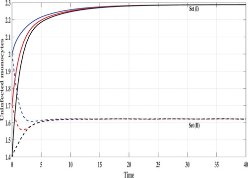
Figure 3. The concentration of latently infected monocytes.

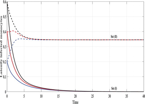
Figure 4. The concentration of actively infected monocytes.

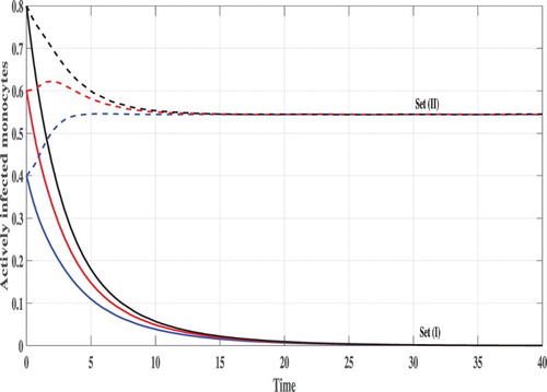
Figure 5. The concentration of free CHIKV particles.

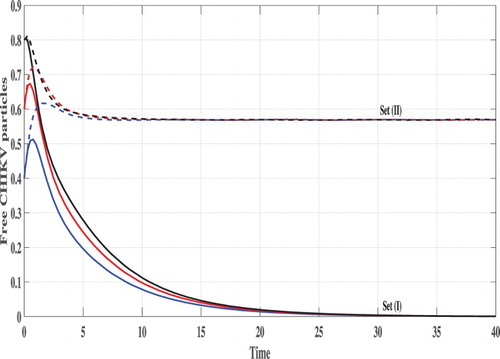
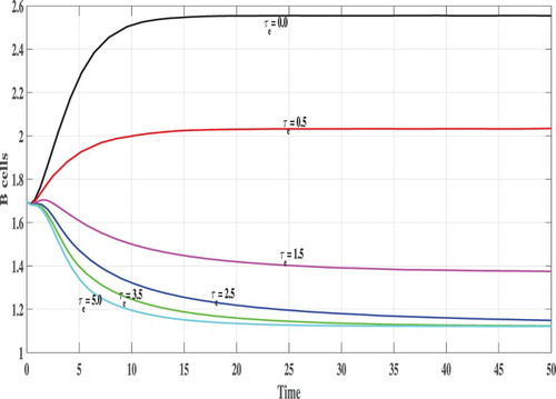
Figure 6. The concentration of B cells.

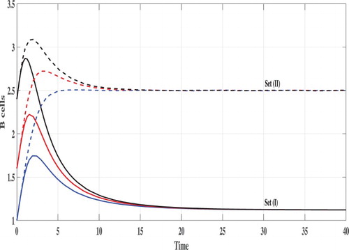
Set (II): We take $b=\mathrm{3.5.}$ Then, we compute ${\mathcal{R}}_0=3.4584>1.$ It means that, the system has two positive steady states $Q_0$ and $Q_1,$ where $Q_1$ is GAS. Figures 2–6 show that the concentration of uninfected monocytes are decreasing, while the concentrations of latently infected monocytes, actively infected monocytes and the CHIKV paticles are increasing. The increasing of the CHIKV paticles will increase the proliferation rate of the B cells and then the concentration of the B cells are also increased. The states of the system converge to the steady state $Q_1=(1.6217,0.3453,0.5443,0.5689,2.4994)$ for all the three initial conditions IC1–IC3. This confirms the result of Theorem 2.2.

Next, we investigate the effect of time delays on the stability of the steady states. We vary the parameter ${\tau }_e,$ and fix b=2.5. The following initial conditions are used: ${\varphi }_1\left(\vartheta \right)=2.0,{\varphi }_2\left(\vartheta \right)=0.2,{\varphi }_3\left(\vartheta \right)=0.3,{\varphi }_4\left(\vartheta \right)=0.3,{\varphi }_5\left(\vartheta \right)=1.7,\vartheta \in \left[-{\tau }_e,0\right].$ In Figures 7–11, we show the evolution of the states of system S, L, I, V and B with respect to the time. We can see that, for lower values of ${\tau }_e$ e.g. ${\tau }_e=0.0$, 0.5, 1.0 and $1.5,$ the corresponding values of ${\mathcal{R}}_0$ satisfy ${\mathcal{R}}_0>1,$ and the trajectory of the system tends to the steady states $Q_1$. This confirms the results of Theorem 2.2 that $Q_1$ is GAS. On the other hand, when ${\tau }_e$ becomes higher e.g. ${\tau }_e=3.5$ and $5.0,$ then ${\mathcal{R}}_0<1$, and the system has one positive steady state $Q_0$ which confirms the results of Theorem 2.1 that $Q_0$ is GAS. In this case, the CHIKV particles are cleared from the body.

Figure 7. The concentration of uninfected monocytes.

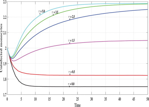
Figure 8. The concentration of latently infected monocytes.

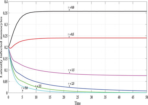
Figure 9. The concentration of actively infected monocytes.

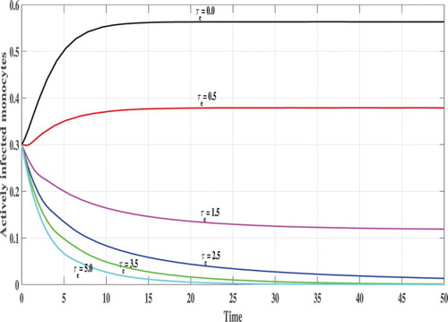
Figure 10. The concentration of free CHIKV particles.

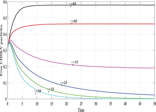
Figure 11. The concentration of B cells.

Let ${\tau }^{cr}$ be the critical value of the parameter ${\tau }_e$, such that ${\mathcal{R}}_0=\frac{m\left(\lambda (1-\rho ){\mathrm{e}}^{-{\delta }_1{\tau }^{cr}}+\rho {\mathrm{e}}^{-{\delta }_2{\tau }^{cr}}(\theta +\lambda )\right)b{S}_0^h}{{\alpha }_2ϵ(\theta +\lambda )(r+q{B}_0)\left({\alpha }_1+S_0^{h_1}\right)}=1.$ From Table 1 we obtain ${\tau }^{cr}=2.3086$. The value of ${\mathcal{R}}_0$ for different values of ${\tau }_e$ are listed in Table 2. We can observed that as ${\tau }_e$ is increased then ${\mathcal{R}}_0$ is decreased. Moreover, we have the following cases:

1. if $0\le {\tau }_e<2.3086$, then $Q_1$ exists and it is GAS,

2. if ${\tau }_e\ge 2.3086$, then $Q_0$ is GAS. It is clearly seen that, an increasing in time delay will stabilize the system around $Q_0$. In terms of biology, the time delay has a similar effect as the antiviral treatment which can be used to eliminate the CHIKV. We observe that, sufficiently large periods of delay reduce CHIKV replication and also clear the virus.

Table 2. The values of steady states, ${\mathcal{R}}_0$ for model (42(42) $\begin{array}{rl}\dot{S}\left(t\right)& =\mu -aS\left(t\right)-\frac{\beta S^h\left(t\right)V\left(t\right)}{\left({\alpha }_1+S^{h_1}\left(t\right)\right)\left({\alpha }_2+V^n\left(t\right)\right)},\end{array}$(42) )–(46(46) $\begin{array}{rl}\dot{B}\left(t\right)& =\eta +cB\left(t\right)V\left(t\right)-\delta B\left(t\right),\end{array}$(46) ) with different values of ${\tau }_e$.

${\tau }_e$	Steady states	$R_0$
0.0	$Q_1=(1.7510,0.3574,0.5634,0.5790,2.5549)$	3.1717
0.5	$Q_1=(1.8243,0.2404,0.3790,0.4627,2.0326)$	2.4703
1.0	$Q_1=(1.9230,0.1474,0.2324,0.3296,1.6470)$	1.9238
1.5	$Q_1=(2.0520,0.0743,0.1171,0.1879,1.3703)$	1.4983
2.0	$Q_1=(2.2085,0.0196,0.0309,0.0543,1.1830)$	1.1669
2.3086	$Q_0=(2.2885,0,0,0,1.1207)$	1.0000
2.5	$Q_0=(2.2885,0,0,0,1.1207)$	0.9088
3.0	$Q_0=(2.2885,0,0,0,1.1207)$	0.7077
3.5	$Q_0=(2.2885,0,0,0,1.1207)$	0.5512
4.0	$Q_0=(2.2885,0,0,0,1.1207)$	0.4293
4.5	$Q_0=(2.2885,0,0,0,1.1207)$	0.3343
5.0	$Q_0=(2.2885,0,0,0,1.1207)$	0.2604

5. Conclusion and discussion

In this paper, we have studied two within-host CHIKV dynamics models with antibody immune response. The incidence rate between the CHIKV and the uninfected monocytes has been modelled by a general nonlinear function Ψ. We have incorporated intracellular discrete or distributed time delays into the model. We have considered two types of infected monocytes, latently infected monocytes (such monocytes contain the CHIKV but are not producing it) and the actively infected monocytes (such monocytes are producing the CHIKV). We have shown that, the solutions of each model are nonnegative and ultimate bounded which ensure the well-posedness of the model. We have derived the basic reproduction number ${\mathcal{R}}_0$ for the model. Sufficient conditions on Ψ and ${\mathcal{R}}_0$ are established which guarantee the existence and global stability of the two steady states, CHIKV-free steady state $Q_0$ and endemic steady state $Q_1$. We have investigated the global stability of the steady states of the model by using Lyapunov method and LaSalle's invariance principle. We have conducted numerical simulations with a specific choice of the function Ψ and have shown that both the theoretical and numerical results are consistent.

The results show that, for the CHIKV infection model, the time delay has a significant effect on both global asymptotic properties of $Q_0$ and global asymptotic properties of $Q_1$. This is due to the dependence of the parameter ${\mathcal{R}}_0$ on the time delay. For model (42(42) $\begin{array}{rl}\dot{S}\left(t\right)& =\mu -aS\left(t\right)-\frac{\beta S^h\left(t\right)V\left(t\right)}{\left({\alpha }_1+S^{h_1}\left(t\right)\right)\left({\alpha }_2+V^n\left(t\right)\right)},\end{array}$(42) )–(46(46) $\begin{array}{rl}\dot{B}\left(t\right)& =\eta +cB\left(t\right)V\left(t\right)-\delta B\left(t\right),\end{array}$(46) ) ${\mathcal{R}}_0$ is given by ${\mathcal{R}}_0({\tau }_1,{\tau }_2)=\frac{m\left(\lambda (1-\rho ){\mathrm{e}}^{-{\delta }_1{\tau }_1}+\rho {\mathrm{e}}^{-{\delta }_2{\tau }_2}(\theta +\lambda )\right)b{S}_0^h}{{\alpha }_2ϵ(\theta +\lambda )(r+q{B}_0)\left({\alpha }_1+S_0^{h_1}\right)},$ which is a decreasing function in both ${\tau }_1$ and ${\tau }_2$. It has a clear meaning that, if the length of the delay is large, infected monocytes may die before it spreads CHIKV due to the small survival probability in the delay period between the infection phase and the CHIKV-producing phase. Clearly, ${\mathcal{R}}_0({\tau }_1,{\tau }_2)<{\mathcal{R}}_0(0,0)$, where ${\mathcal{R}}_0(0,0)$ is the basic reproduction number of system (42(42) $\begin{array}{rl}\dot{S}\left(t\right)& =\mu -aS\left(t\right)-\frac{\beta S^h\left(t\right)V\left(t\right)}{\left({\alpha }_1+S^{h_1}\left(t\right)\right)\left({\alpha }_2+V^n\left(t\right)\right)},\end{array}$(42) )–(46(46) $\begin{array}{rl}\dot{B}\left(t\right)& =\eta +cB\left(t\right)V\left(t\right)-\delta B\left(t\right),\end{array}$(46) ) without delay. It follows that, the system with delay is more stabilizable abound $Q_0$ than that without delay.

Acknowledgments

This article was funded by the Deanship of Scientific Research (DSR) at King Abdulaziz University, Jeddah. The authors, therefore, acknowledge with thanks DSR for technical and financial support.

Disclosure statement

No potential conflict of interest was reported by the authors.

References

- A. Alshorman, X. Wang, J. Meyer, and L. Rong, Analysis of HIV models with two time delays, J. Biol. Dyn. 11(S1) (2017), pp. 40–64. doi: 10.1080/17513758.2016.1148202
- C. Connell McCluskey and Y. Yang, Global stability of a diffusive virus dynamics model with general incidence function and time delay, Nonlinear Anal. 25 (2015), pp. 64–78. doi: 10.1016/j.nonrwa.2015.03.002
- Y. Dumont and F. Chiroleu, Vector control for the chikungunya disease, Math. Biosci. Eng. 7 (2010), pp. 313–345. doi: 10.3934/mbe.2010.7.313
- Y. Dumont and J.M. Tchuenche, Mathematical studies on the sterile insect technique for the chikungunya disease and aedes albopictus, J. Math. Biol. 65(5) (2012), pp. 809–854. doi: 10.1007/s00285-011-0477-6
- Y. Dumont, F. Chiroleu, and C. Domerg, On a temporal model for the chikungunya disease: Modeling, theory and numerics, Math. Biosci. 213 (2008), pp. 80–91. doi: 10.1016/j.mbs.2008.02.008
- A.M. Elaiw, Global properties of a class of HIV models, Nonlinear Anal. 11 (2010), pp. 2253–2263. doi: 10.1016/j.nonrwa.2009.07.001
- A.M. Elaiw, Global properties of a class of virus infection models with multitarget cells, Nonlinear Dyn. 69(1–2) (2012), pp. 423–435. doi: 10.1007/s11071-011-0275-0
- A.M. Elaiw, Global stability analysis of humoral immunity virus dynamics model including latently infected cells, J. Biol. Dyn. 9(1) (2015), pp. 215–228. doi: 10.1080/17513758.2015.1056846
- A.M. Elaiw and N.A. Almuallem, Global dynamics of delay-distributed HIV infection models with differential drug efficacy in cocirculating target cells, Math. Methods Appl. Sci. 39 (2016), pp. 4–31. doi: 10.1002/mma.3453
- A.M. Elaiw and N.H. AlShamrani, Global properties of nonlinear humoral immunity viral infection models, Int. J. Biomath. 8(5) (2015). Article ID 1550058. doi: 10.1142/S1793524515500588
- A.M. Elaiw and N.H. AlShamrani, Global stability of humoral immunity virus dynamics models with nonlinear infection rate and removal, Nonlinear Anal. 26 (2015), pp. 161–190. doi: 10.1016/j.nonrwa.2015.05.007
- A.M. Elaiw and N.H. AlShamrani, Stability of a general delay-distributed virus dynamics model with multi-staged infected progression and immune response, Math. Methods Appl. Sci. 40(3) (2017), pp. 699–719. doi: 10.1002/mma.4002
- A.M. Elaiw and N.H. AlShamrani, Stability of latent pathogen infection model with adaptive immunity and delays, J. Integr. Neurosci 2018. DOI:10.3233/JIN-180087.
- A.M. Elaiw and A.A. Raezah, Stability of general virus dynamics models with both cellular and viral infections and delays, Math. Methods Appl. Sci. 40(16) (2017), pp. 5863–5880. doi: 10.1002/mma.4436
- A.M. Elaiw and S.A. Azoz, Global properties of a class of HIV infection models with Beddington-DeAngelis functional response, Math. Methods Appl. Sci. 36 (2013), pp. 383–394. doi: 10.1002/mma.2596
- A.M. Elaiw, I.A. Hassanien, and S.A. Azoz, Global stability of HIV infection models with intracellular delays, J. Korean Math. Soc. 49(4) (2012), pp. 779–794. doi: 10.4134/JKMS.2012.49.4.779
- A.M. Elaiw, A. Raezah, and A.S. Alofi, Effect of humoral immunity on HIV-1 dynamics with virus-to-target and infected-to-target infections, AIP Adv. 6(8) (2016). Article ID 085204. doi: 10.1063/1.4960987
- A.M. Elaiw, N.H. AlShamrani, and K. Hattaf, Dynamical behaviors of a general humoral immunity viral infection model with distributed invasion and production, Int. J. Biomath. 10(3) (2017). Article ID 1750035. doi: 10.1142/S1793524517500358
- A.M. Elaiw, A.A. Raezah, and K. Hattaf, Stability of HIV-1 infection with saturated virus-target and infected-target incidences and CTL immune response, Int. J. Biomath. 10(5) (2017). Article ID 1750070. doi: 10.1142/S179352451750070X
- A.M. Elaiw, N.H. AlShamrani, and A.S. Alofi, Stability of CTL immunity pathogen dynamics model with capsids and distributed delay, AIP Adv. 7 (2017). Article ID 125111.
- A.M. Elaiw, A. Raezah, and A. Alofi, Stability of a general delayed virus dynamics model with humoral immunity and cellular infection, AIP Adv. 7(6) (2017). Article ID 065210. doi: 10.1063/1.4989569
- A.M. Elaiw, E. Kh. Elnahary, and A.A. Raezah, Effect of cellular reservoirs and delays on the global dynamics of HIV, Adv. Difference Equ. 2018 (2018), p. 85. doi: 10.1186/s13662-018-1523-0
- A.M. Elaiw, A.A. Raezah, and B.S. Alofi, Dynamics of delayed pathogen infection models with pathogenic and cellular infections and immune impairment, AIP Adv. 8 (2018). Article ID 025323.
- L. Gibelli, A. Elaiw, M.A. Alghamdi, and A.M. Althiabi, Heterogeneous population dynamics of active particles: Progression, mutations, and selection dynamics, Math. Models Methods Appl. Sci. 27 (2017), pp. 617–640. doi: 10.1142/S0218202517500117
- J.K. Hale and S.M. Verduyn Lunel, Introduction to Functional Differential Equations, Springer Verlag, New York, 1993.
- K. Hattaf, N. Yousfi, and A. Tridane, Mathematical analysis of a virus dynamics model with general incidence rate and cure rate, Nonlinear Anal. Real World Appl. 13(4) (2012), pp. 1866–1872. doi: 10.1016/j.nonrwa.2011.12.015
- G. Huang, Y. Takeuchi, and W. Ma, Lyapunov functionals for delay differential equations model of viral infections, SIAM J. Appl. Math. 70(7) (2010), pp. 2693–2708. doi: 10.1137/090780821
- D. Huang, X. Zhang, Y. Guo, and H. Wang, Analysis of an HIV infection model with treatments and delayed immune response, Appl. Math. Model. 40(4) (2016), pp. 3081–3089. doi: 10.1016/j.apm.2015.10.003
- X. Li and S. Fu, Global stability of a virus dynamics model with intracellular delay and CTL immune response, Math. Methods Appl. Sci. 38 (2015), pp. 420–430. doi: 10.1002/mma.3078
- B. Li, Y. Chen, X. Lu, and S. Liu, A delayed HIV-1 model with virus waning term, Math. Biosci. Eng. 13 (2016), pp. 135–157. doi: 10.3934/mbe.2016.13.135
- X. Liu and P. Stechlinski, Application of control strategies to a seasonal model of chikungunya disease, Appl. Math. Model. 39 (2015), pp. 3194–3220. doi: 10.1016/j.apm.2014.10.035
- S. Liu and L. Wang, Global stability of an HIV-1 model with distributed intracellular delays and a combination therapy, Math. Biosci. Eng. 7(3) (2010), pp. 675–685. doi: 10.3934/mbe.2010.7.675
- K.M. Long and M.T. Heise, Protective and pathogenic responses to Chikungunya virus infection, Curr. Trop. Med. Rep. 2(1) (2015), pp. 13–21. doi: 10.1007/s40475-015-0037-z
- F.M. Lum and L.F.P. Ng, Cellular and molecular mechanisms of Chikungunya pathogenesis, Antiviral Res. 120 (2015), pp. 165–174. doi: 10.1016/j.antiviral.2015.06.009
- C.A. Manore, K.S. Hickmann, S. Xu, H.J. Wearing, and J.M. Hyman, Comparing dengue and chikungunya emergence and endemic transmission in A. aegypti and A. albopictus, J. Theoret. Biol. 356 (2014), pp. 174–191. doi: 10.1016/j.jtbi.2014.04.033
- C. Monica and M. Pitchaimani, Analysis of stability and Hopf bifurcation for HIV-1 dynamics with PI and three intracellular delays, Nonlinear Anal. 27 (2016), pp. 55–69. doi: 10.1016/j.nonrwa.2015.07.014
- D. Moulay, M. Aziz-Alaoui, and M. Cadivel, The chikungunya disease: Modeling, vector and transmission global dynamics, Math. Biosci. 229 (2011), pp. 50–63. doi: 10.1016/j.mbs.2010.10.008
- D. Moulay, M. Aziz-Alaoui, and H.D. Kwon, Optimal control of chikungunya disease: Larvae reduction, treatment and prevention, Math. Biosci. Eng. 9 (2012), pp. 369–392. doi: 10.3934/mbe.2012.9.369
- A.U. Neumann, N.P. Lam, H. Dahari, D.R. Gretch, T.E. Wiley, T.J Layden, and A.S. Perelson, Hepatitis C viral dynamics in vivo and the antiviral efficacy of interferon-alpha therapy, Science 282 (1998), pp. 103–107. doi: 10.1126/science.282.5386.103
- P.K. Roy, A.N. Chatterjee, D. Greenhalgh, and Q.J.A. Khan, Long term dynamics in a mathematical model of HIV-1 infection with delay in different variants of the basic drug therapy model, Nonlinear Anal. 14 (2013), pp. 1621–1633. doi: 10.1016/j.nonrwa.2012.10.021
- X. Shi, X. Zhou, and X. Son, Dynamical behavior of a delay virus dynamics model with CTL immune response, Nonlinear Anal. 11 (2010), pp. 1795–1809. doi: 10.1016/j.nonrwa.2009.04.005
- H. Shu, L. Wang, and J. Watmough, Global stability of a nonlinear viral infection model with infinitely distributed intracellular delays and CTL imune responses, SIAM J. Appl. Math. 73(3) (2013), pp. 1280–1302. doi: 10.1137/120896463
- Y. Wang and X. Liu, Stability and Hopf bifurcation of a within-host chikungunya virus infection model with two delays, Math. Comput. Simul. 138 (2017), pp. 31–48. doi: 10.1016/j.matcom.2016.12.011
- L. Wang, M.Y. Li, and D. Kirschner, Mathematical analysis of the global dynamics of a model for HTLV-I infection and ATL progression, Math. Biosci. 179 (2002), pp. 207–217. doi: 10.1016/S0025-5564(02)00103-7
- K. Wang, A. Fan, and A. Torres, Global properties of an improved hepatitis B virus model, Nonlinear Anal. 11 (2010), pp. 3131–3138. doi: 10.1016/j.nonrwa.2009.11.008
- X. Wang, S. Tang, X. Song, and L. Rong, Mathematical analysis of an HIV latent infection model including both virus-to-cell infection and cell-to-cell transmission, J. Biol. Dyn. 11(S2) (2017), pp. 455–483. doi: 10.1080/17513758.2016.1242784
- J. Wang, J. Lang, and X. Zou, Analysis of an age structured HIV infection model with virus-to-cell infection and cell-to-cell transmission, Nonlinear Anal. 34 (2017), pp. 75–96. doi: 10.1016/j.nonrwa.2016.08.001
- L. Yakob and A.C. Clements, A mathematical model of chikungunya dynamics and control: The major epidemic on Reunion Island, PLoS One 8 (2013), p. e57448. doi: 10.1371/journal.pone.0057448