Modeling the seasonality of Methicillin-resistant Staphylococcus aureus infections in hospitals with environmental contamination

ABSTRACT

A deterministic mathematical model with periodic antibiotic prescribing rate is constructed to study the seasonality of Methicillin-resistant Staphylococcus aureus (MRSA) infections taking antibiotic exposure and environmental contamination into consideration. The basic reproduction number $R_0$ for the periodic model is calculated under the assumption that there are only uncolonized patients with antibiotic exposure at admission. Sensitivity analysis of $R_0$ with respect to some essential parameters is performed. It is shown that the infection would go to extinction if the basic reproduction number is less than unity and would persist if it is greater than unity. Numerical simulations indicate that environmental cleaning is the most important intervention to control the infection, which emphasizes the effect of environmental contamination in MRSA infections. It is also important to highlight the importance of effective antimicrobial stewardship programmes, increase active screening at admission and subsequent isolation of positive cases, and treat patients quickly and efficiently.

KEYWORDS:

• Seasonality
• basic reproduction number
• antibiotic exposure
• environmental contamination
• persistent

1. Introduction

Methicillin-resistant Staphylococcus aureus (MRSA), a type of staph bacteria first discovered in 1961, is one of the most common causes of hospital-acquired infections. As a considerable threat to global public health, MRSA causes many hard-to-treat infections such as serious skin infections, brain abscess (central nervous system infection), endophthalmitis, pneumonia (lung infection), and bloodstream infections. We usually treat staph bacteria with antibiotics, however, as antibiotics are abused to be prescribed to inhibit these kinds of bacteria infections, so far MRSA has been resistant to many common antibiotics such as methicillin, oxacillin, penicillin, and amoxicillin. Based on a Centers for Disease Control and Prevention (CDC) report [5], 30–50$\mathrm{\%}$ of antibiotics patients accepted in hospitals are unnecessary or inappropriate. Even though some antibiotics still work, MRSA is constantly adapting, which makes researchers difficult to keep developing new antibiotics. Hence whether a patient has antibiotic exposure or not is kind of important for his or her treatment. In fact, many studies observe that patients with antibiotic exposure tend to be more likely to be colonized by MRSA, which results in a lengthier duration in hospitals, a higher chance of failed treatment, a more expensive cost, a larger shedding rate of bacteria to environment, and even a higher mortality of death [6,10,23,24]. Hence it is necessary to consider antibiotic exposure and use of antibiotics in hospitals as influential factors in the transmission of MRSA.

Furthermore, in recent decades seasonal variation of MRSA infections in the hospital settings has been widely observed, especially in surgical wound, skin and soft tissue, urine, and respiratory tract in young children [12,14,17,18,21,22]. Reasons for this seasonal variation of MRSA infections in hospital are very complicated and still controversial. Previous studies believe that the seasonality involves temperature variation, insect bites, seasonal influenza, community-associated MRSA (CA-MRSA) infection, school season, seasonal community antibiotic use, which may result in a seasonal pattern of antibiotic prescriptions in hospitals. Especially, in the work of Sun et al. [22], seasonality in the prescription data was found (see Figure 1). Moreover, they performed a seasonal decomposition analysis for the MRSA isolates and found out that both fluoroquinolone prescriptions and the percentage of MRSA isolates that were resistant to ciprofloxacin peaked in the winter. Similar results were found for both the percentage of MRSA isolates resistant to clindamycin and macrolide/lincosamide prescriptions (see Figure 2). Though this does not totally reflect the antibiotic usage in hospitals, [21,22] indicate that the usage of antibiotics in hospitals should also fluctuate seasonally. We believe that the seasonal pattern of antibiotic consumption implies the seasonal circulation of pathogens, which could induce seasonal risk of infections for hospitalized patients due to their weakened immune systems, and thus results in seasonal antibiotic consumption rates among hospitalized patients. Therefore, in our model we assume the antibiotic prescribing rate as a periodic function depending on time t, which has a period of 365 days and represents that antibiotic prescribing rate increases starting at the beginning of August, gains a peak in winter and then decreases starting at the beginning of February according to the data shown in Figure 2.

Figure 1. Number of prescriptions for antibiotic drug classes, by month. Source: IMS Health, Xponent, 1999–2007. Abbreviation: TMP/Sulfra, trimethoprim/sulfamethoxazole [22].

Figure 2. (a) Seasonal pattern of fluoroquinolone prescriptions and MRSA isolates resistant to ciprofloxacin; Mean monthly seasonal variation for fluoroquinolone prescriptions and MRSA isolates resistant to clindamycin for inpatient, outpatient and combined isolates as calculated by STL method. Prescription data source: IMS Health, Xponent, 1999–2007; Resistance data source: The Surveillance Network (TSN) Database-USA (Focus Diagnostics, Herndon, VA, USA) and (b) Seasonal pattern of macrolide and lincosamide prescriptions and MRSA isolates resistant to ciprofloxacin; Mean monthly seasonal variation for macrolide and lincosamide prescriptions and MRSA isolates resistant to clindamycin for inpatient, outpatient and combined isolates as calculated by STL method. Prescription data source: IMS Health, Xponent, 1999–2007; Resistance data source: The Surveillance Network (TSN) Database-USA (Focus Diagnostics, Herndon, VA, USA) [22].

Mathematical modelling, as a powerful tool in quantifying the complex and numerous factors, has been widely developed to explore the transmission of MRSA [1,3,6-9,11,25,26,28]. In their work, the direct patient-healthcare worker transmission is shown to be an essential factor in the transmission of MRSA in hospitals, as well as the indirect transmission via environmental contamination based on the observation that MRSA has the ability to be alive for days, weeks or even months on environmental surfaces in healthcare facilities, doors, and gowns. To the best of our knowledge, no model has been developed to address the seasonality in the transmission of MRSA. Studying seasonality of MRSA infections is helpful in developing efficient control programmes, lowering the long-term health risks, and distributing public resources.

We organize the paper as follows. We develop a periodic mathematical model to describe a comprehensive transmission of MRSA in Section 2. In Section 3, boundedness and positivity of solutions, the basic reproduction number, the extinction and uniform persistence of infections are analyzed. Simulations and discussion of the model behaviours and sensitive analysis of the basic reproduction number are given in the last two sections.

2. The periodic deterministic model

In order to describe the seasonal transmission of MRSA by a mathematical model, we first denote the patients, health-care workers (HCWS) and free-living bacteria in the environment as the following seven compartments [16]:

• $P_u\left(t\right)=\text{number of uncolonized patients without antibiotic exposure at time }t$.

• $P_{uA}\left(t\right)=\text{number of uncolonized patients with antibiotic exposure at time }t$.

• $P_c\left(t\right)=\text{number of colonized patients without antibiotic exposure at time }t$.

• $P_{cA}\left(t\right)=\text{number of colonized patients with antibiotic exposure at time }t$.

• $H_u\left(t\right)\text{number of uncontaminated health care workers at time }t$.

• $H_c\left(t\right)=\text{number of contaminated health care workers at time }t$.

• $B_e\left(t\right)=\text{number of the free-living bacteria in the environment at time }t$.

The flowchart describing the transmission dynamics of MRSA in hospitals among these seven compartments is given in Figure 3. Our periodic deterministic model is derived based on the following assumptions and descriptions:

1. We assume that a patient would have antibiotic exposure if he or she has received antibiotics within the month at admission or is currently receiving antibiotic treatment in the hospital.

2. Based on the seasonal pattern of antibiotic usage found in Sun et al. [22], we use a periodic function $ϵ\left(t\right)={ϵ}_0(1+{ϵ}_1\sin (\left(2\pi /365\right)(t-240)\left)\right)$ to describe the antibiotic prescription rate in the hospital. $ϵ\left(t\right)$ has a period of 365 days, and represents that antibiotic prescription rate increases starting at the beginning of August, gains a peak in winter and then decreases starting at the beginning of February according to the data shown in Figures 1 and 2. ${ϵ}_0$ is the baseline antibiotic prescription rate and ${ϵ}_1$ is the magnitude of change.

3. The free-living bacteria are uniformly distributed in the environment.

4. The total number of patients in a unit is a constant $N_p$. That is equivalent to say that patients are admitted at a total rate $\mathrm{\Omega }\left(t\right)={\gamma }_u{P}_u+{\gamma }_c{P}_c+{\gamma }_{uA}{P}_{uA}+{\gamma }_{cA}{P}_{cA}$, where ${\gamma }_u,{\gamma }_{uA},{\gamma }_c,$ and ${\gamma }_{cA}$ are the corresponding discharge rates of patients from these four compartments. We also denote ${\theta }_u,{\theta }_{uA},{\theta }_c,{\theta }_{cA}$ as the corresponding proportion of patients $P_u,P_{uA},P_c,P_{cA}$ at admission. It was estimated that the fraction of patients with antibiotic exposure of new admission to be 0.38, i.e. ${\theta }_{uA}+{\theta }_{cA}$=0.38 [6,15].

5. The total number of health-care workers is a constant $N_h$.

6. We assume that the bacterial reproduction cannot occur due to lack of proper condition in the hospital, even though the free-living bacteria are able to survive in the environment for a long time. As a result, shedding from colonized patients is one of the key transmission of bacteria to contaminate environment ${\upsilon }_p{P}_c+{\upsilon }_{pA}{P}_{cA}$. ${\upsilon }_p$, and ${\upsilon }_{pA}$ are the shedding rate of bacteria from patients without or with antibiotic exposure, respectively. In addition, when the contaminated HCWs touch the environmental surfaces such as door handles, health facilities, bedding, they leave bacteria there ${\upsilon }_h{H}_c$, which is another way to contaminate the environment. Of course, hospitals always have a standard cleaning rate or disinfection rate ${\gamma }_b$.

7. We assume that there is no contact between patients, which means that if an uncolonized patient without antibiotic exposure becomes colonized without antibiotic exposure, he/she either contacts contaminated HCWs at rate ${\alpha }_p{\beta }_p(1-\eta )P_u{H}_c$ or touches the contaminated environment at rate ${\kappa }_p{P}_u{B}_e$. A similar process happens when an uncolonized patient with antibiotic exposure becomes colonized with antibiotic exposure at rate ${\alpha }_p{\beta }_{pA}(1-\eta )P_{uA}{H}_c+{\kappa }_{pA}{P}_{uA}{B}_e$. ${\alpha }_p$ is the contact rate per day, ${\beta }_p$ and ${\beta }_{pA}$ are the chance of colonization per contact for uncolonized patients without or with antibiotic exposure, respectively, η is the hand hygiene compliance, ${\kappa }_p$ and ${\kappa }_{pA}$ are the chance of colonization by touching contaminated environment for uncolonized patients without or with antibiotic exposure, respectively. Besides, when an uncolonized patient without antibiotic exposure is accepting an antibiotic treatment for other diseases, which is the reason for his/her hospitalization, he/she then becomes uncolonized patients with antibiotic exposure $ϵ\left(t\right)P_u$. That is similar to how a colonized patient without antibiotic exposure becomes colonized with antibiotic exposure $ϵ\left(t\right)P_c$. Note that an uncolonized patient without antibiotic exposure cannot move to the colonized with antibiotic exposure in one step.

8. An uncontaminated HCW becomes contaminated when he/she contacts colonized patients or touches contaminated environmental surfaces at rate ${\alpha }_p{\beta }_h(1-\eta )P_c{H}_u+{\alpha }_p{\beta }_{hA}(1-\eta )P_{cA}{H}_u$, where ${\beta }_h,{\beta }_{hA}$ are chance of contamination per contact with $P_c$ or $P_{cA}$, respectively. HCWs have a decontaminated rate ${\mu }_c$ to move from contaminated state to uncontaminated state.

9. Antibiotics can not only kill the bad bacteria that make patients sick, but also commensal bacteria, this may disturb the balance of patients' commensal microbiota. Then patients with prior antibiotic exposure are more likely to have a higher colonization rate of MRSA, so we assume ${\beta }_{pA}\ge {\beta }_p$. In addition, by previous studies [6,13], we estimate that uncolonized patients with antibiotic exposure are 1.67 times more vulnerable than uncolonized patients without antibiotic exposure, i.e. ${\beta }_{pA}=1.67\times {\beta }_p$. Moreover, patients with recent antibiotic exposure are more likely to experience adverse effects or new health problems (such as gastrointestinal symptoms, respiratory infections, skin rashes, and so on); and a higher probability of treatment failure because of the acquisition of resistance elements, which lead to lengthier hospital stays. So we assume that ${\gamma }_{cA}^{-1}\ge {\gamma }_c^{-1}\ge {\gamma }_{uA}^{-1}\ge {\gamma }_u^{-1}$. We also follow the assumptions and parametrizions from [6,13,25] for the values of ${\beta }_h,{\beta }_{hA},{\upsilon }_p,{\upsilon }_{pA},{\upsilon }_h,{\kappa }_p,{\kappa }_{pA},{\kappa }_h$ as shown in Table 1.

Figure 3. Transmission flowchart of MRSA among patients, health-care works and environment.

Table 1. Parameters and descriptions.

Parameter	Description	Parameter estimate	Reference
${ϵ}_0$	antibiotic prescription rate	0.12	[13,20]
${ϵ}_1$	magnitude of change of antibiotic prescription rate	0.25	[22]
${\theta }_u$	proportion of $P_u$ on admission	0.617	[6,13]
${\theta }_{uA}$	proportion of $P_{uA}$ on admission	0.349	[6,15]
${\theta }_c$	proportion of $P_c$ on admission	0.003	[6,13]
${\theta }_{cA}$	proportion of $P_{cA}$on admission	0.031	[6,15]
${\gamma }_u$	discharge rate of $P_u$ (1/day)	0.2	[6]
${\gamma }_{uA}$	discharge rate of $P_{uA}$ (1/day)	0.2	[6]
${\gamma }_c$	discharge rate of $P_c$ (1/day)	0.06	[13]
${\gamma }_{cA}$	discharge rate of $P_{cA}$ (1/day)	0.055	[6,13]
${\gamma }_b$	disinfection rate of environment	0.7	[26]
${\alpha }_p$	Contact rate	0.0435	[26]
${\beta }_p$	probability of colonization for $P_u$ after a contact with $H_c$	0.42	[26]
${\beta }_{pA}$	probability of colonization for $P_{uA}$ after a contact with $H_c$	0.42*1.67	[6,13]
${\beta }_h$	probability of contamination for HCW after a contact with $P_c$	0.2	[6,26]
${\beta }_{hA}$	probability of contamination for HCW after a contact with $P_{cA}$	0.25	[6]
η	hand hygiene compliance with HCWs	0.4	[26]
${\mu }_c$	decontaminated rate of HCWs	24	[26]
${\upsilon }_p$	contamination(shedding) rate to the environment from $P_c$	235	[26]
${\upsilon }_{pA}$	contamination(shedding) rate to theenvironment from $P_{cA}$	470	[13,28]
${\upsilon }_h$	contamination rate to the environment by contaminated HCWs	235	[26]
${\kappa }_p$	colonization rate from environment for $P_u$	0.000004	[26]
${\kappa }_{pA}$	colonization rate from environment for $P_{uA}$	0.000005	[6,26]
${\kappa }_h$	colonization rate from environment for uncontaminated HCWs	0.00001	[26]
$N_p$	total number of patients	23	[26]
$N_h$	total number of HCWs	23	[26]

Detailed parameter values are given in Table 1. We hence formulate the periodic mathematical model as follows: (1) $\begin{array}{r}\begin{array}{rl}\frac{\mathrm{d}{P}_u}{\mathrm{d}t}& ={\theta }_u\mathrm{\Omega }\left(t\right)-{\alpha }_p{\beta }_p(1-\eta )P_u{H}_c-{\kappa }_p{P}_u{B}_e-{\gamma }_u{P}_u-ϵ\left(t\right)P_u,\\ \frac{\mathrm{d}{P}_c}{\mathrm{d}t}& ={\theta }_c\mathrm{\Omega }\left(t\right)+{\alpha }_p{\beta }_p(1-\eta )P_u{H}_c+{\kappa }_p{P}_u{B}_e-{\gamma }_c{P}_c-ϵ\left(t\right)P_c,\\ \frac{\mathrm{d}{P}_{uA}}{\mathrm{d}t}& ={\theta }_{uA}\mathrm{\Omega }\left(t\right)-{\alpha }_p{\beta }_{pA}(1-\eta )P_{uA}{H}_c-{\kappa }_{pA}{P}_{uA}{B}_e-{\gamma }_{uA}{P}_{uA}+ϵ\left(t\right)P_u,\\ \frac{\mathrm{d}{P}_{cA}}{\mathrm{d}t}& ={\theta }_{cA}\mathrm{\Omega }\left(t\right)+{\alpha }_p{\beta }_{pA}(1-\eta )P_{uA}{H}_c+{\kappa }_{pA}{P}_{uA}{B}_e-{\gamma }_{cA}{P}_{cA}+ϵ\left(t\right)P_c,\\ \frac{\mathrm{d}{H}_u}{\mathrm{d}t}& =-{\alpha }_p{\beta }_h(1-\eta )P_c{H}_u-{\alpha }_p{\beta }_{hA}(1-\eta )P_{cA}{H}_u-{\kappa }_h{H}_u{B}_e+{\mu }_c{H}_c,\\ \frac{\mathrm{d}{H}_c}{\mathrm{d}t}& ={\alpha }_p{\beta }_h(1-\eta )P_c{H}_u+{\alpha }_p{\beta }_{hA}(1-\eta )P_{cA}{H}_u+{\kappa }_h{H}_u{B}_e-{\mu }_c{H}_c,\\ \frac{\mathrm{d}{B}_e}{\mathrm{d}t}& ={\upsilon }_p{P}_c+{\upsilon }_{pA}{P}_{cA}+{\upsilon }_h{H}_c-{\gamma }_b{B}_e\end{array}\end{array}$(1) with initial conditions $P_u\left(0\right)=P_u^0$, $P_{uA}\left(0\right)=P_{uA}^0$, $P_c\left(0\right)=P_c^0$, $P_{cA}\left(0\right)=P_{cA}^0$, $H_u\left(0\right)=H_u^0$, $H_c\left(0\right)=H_c^0$, $B_e\left(0\right)=B_e^0,$ where $\mathrm{\Omega }\left(t\right)=({\gamma }_u{P}_u+{\gamma }_c{P}_c+{\gamma }_{uA}{P}_{uA}+{\gamma }_{cA}{P}_{cA})$ and $ϵ\left(t\right)={ϵ}_0(1+{ϵ}_1\sin (\left(2\pi /365\right)(t-240)\left)\right).$

3. Mathematical analysis

3.1. Basic reproduction number

The basic reproduction number $R_0$ for the periodic deterministic model (1(1) $\begin{array}{r}\begin{array}{rl}\frac{\mathrm{d}{P}_u}{\mathrm{d}t}& ={\theta }_u\mathrm{\Omega }\left(t\right)-{\alpha }_p{\beta }_p(1-\eta )P_u{H}_c-{\kappa }_p{P}_u{B}_e-{\gamma }_u{P}_u-ϵ\left(t\right)P_u,\\ \frac{\mathrm{d}{P}_c}{\mathrm{d}t}& ={\theta }_c\mathrm{\Omega }\left(t\right)+{\alpha }_p{\beta }_p(1-\eta )P_u{H}_c+{\kappa }_p{P}_u{B}_e-{\gamma }_c{P}_c-ϵ\left(t\right)P_c,\\ \frac{\mathrm{d}{P}_{uA}}{\mathrm{d}t}& ={\theta }_{uA}\mathrm{\Omega }\left(t\right)-{\alpha }_p{\beta }_{pA}(1-\eta )P_{uA}{H}_c-{\kappa }_{pA}{P}_{uA}{B}_e-{\gamma }_{uA}{P}_{uA}+ϵ\left(t\right)P_u,\\ \frac{\mathrm{d}{P}_{cA}}{\mathrm{d}t}& ={\theta }_{cA}\mathrm{\Omega }\left(t\right)+{\alpha }_p{\beta }_{pA}(1-\eta )P_{uA}{H}_c+{\kappa }_{pA}{P}_{uA}{B}_e-{\gamma }_{cA}{P}_{cA}+ϵ\left(t\right)P_c,\\ \frac{\mathrm{d}{H}_u}{\mathrm{d}t}& =-{\alpha }_p{\beta }_h(1-\eta )P_c{H}_u-{\alpha }_p{\beta }_{hA}(1-\eta )P_{cA}{H}_u-{\kappa }_h{H}_u{B}_e+{\mu }_c{H}_c,\\ \frac{\mathrm{d}{H}_c}{\mathrm{d}t}& ={\alpha }_p{\beta }_h(1-\eta )P_c{H}_u+{\alpha }_p{\beta }_{hA}(1-\eta )P_{cA}{H}_u+{\kappa }_h{H}_u{B}_e-{\mu }_c{H}_c,\\ \frac{\mathrm{d}{B}_e}{\mathrm{d}t}& ={\upsilon }_p{P}_c+{\upsilon }_{pA}{P}_{cA}+{\upsilon }_h{H}_c-{\gamma }_b{B}_e\end{array}\end{array}$(1) ) is constructed according to the definition in Baca$\ddot{e}$r and Guenaoui [2] and follow the general calculation procedure in Wang and Zhao [27]. When ${\theta }_u$=0, ${\theta }_c$=0, and ${\theta }_{cA}$=0, that is only uncolonized patients with antibiotic exposure are admitted into hospital, the infection-free infection (IFE) is defined as $E_0=(P_u,P_c,P_{uA},P_{cA},H_u,H_c,B_e)=(0,0,N_p,0,N_h,0,0),$ We can rewrite the variables of periodic ODE system (1(1) $\begin{array}{r}\begin{array}{rl}\frac{\mathrm{d}{P}_u}{\mathrm{d}t}& ={\theta }_u\mathrm{\Omega }\left(t\right)-{\alpha }_p{\beta }_p(1-\eta )P_u{H}_c-{\kappa }_p{P}_u{B}_e-{\gamma }_u{P}_u-ϵ\left(t\right)P_u,\\ \frac{\mathrm{d}{P}_c}{\mathrm{d}t}& ={\theta }_c\mathrm{\Omega }\left(t\right)+{\alpha }_p{\beta }_p(1-\eta )P_u{H}_c+{\kappa }_p{P}_u{B}_e-{\gamma }_c{P}_c-ϵ\left(t\right)P_c,\\ \frac{\mathrm{d}{P}_{uA}}{\mathrm{d}t}& ={\theta }_{uA}\mathrm{\Omega }\left(t\right)-{\alpha }_p{\beta }_{pA}(1-\eta )P_{uA}{H}_c-{\kappa }_{pA}{P}_{uA}{B}_e-{\gamma }_{uA}{P}_{uA}+ϵ\left(t\right)P_u,\\ \frac{\mathrm{d}{P}_{cA}}{\mathrm{d}t}& ={\theta }_{cA}\mathrm{\Omega }\left(t\right)+{\alpha }_p{\beta }_{pA}(1-\eta )P_{uA}{H}_c+{\kappa }_{pA}{P}_{uA}{B}_e-{\gamma }_{cA}{P}_{cA}+ϵ\left(t\right)P_c,\\ \frac{\mathrm{d}{H}_u}{\mathrm{d}t}& =-{\alpha }_p{\beta }_h(1-\eta )P_c{H}_u-{\alpha }_p{\beta }_{hA}(1-\eta )P_{cA}{H}_u-{\kappa }_h{H}_u{B}_e+{\mu }_c{H}_c,\\ \frac{\mathrm{d}{H}_c}{\mathrm{d}t}& ={\alpha }_p{\beta }_h(1-\eta )P_c{H}_u+{\alpha }_p{\beta }_{hA}(1-\eta )P_{cA}{H}_u+{\kappa }_h{H}_u{B}_e-{\mu }_c{H}_c,\\ \frac{\mathrm{d}{B}_e}{\mathrm{d}t}& ={\upsilon }_p{P}_c+{\upsilon }_{pA}{P}_{cA}+{\upsilon }_h{H}_c-{\gamma }_b{B}_e\end{array}\end{array}$(1) ) as a vector $E_0=(P_c,P_{cA},H_c,B_e,P_u,P_{uA},H_u)=(0,0,0,0,0,N_p,N_h)$. Following the general calculation procedure in Wang and Zhao [27], we have $\begin{array}{rl}\mathcal{F}& =\left(\begin{array}{c}{\alpha }_p{\beta }_p(1-\eta )P_u{H}_c+{\kappa }_p{P}_u{B}_e\\ {\alpha }_p{\beta }_{pA}(1-\eta )P_{uA}{H}_c+{\kappa }_{pA}{P}_{uA}{B}_e\\ {\alpha }_p{\beta }_h(1-\eta )P_c{H}_u+{\alpha }_p{\beta }_{hA}(1-\eta )P_{cA}{H}_u+{\kappa }_h{H}_u{B}_e\\ 0\\ 0\\ 0\\ 0\end{array}\right),\\ \mathcal{V}& =\left(\begin{array}{c}{\gamma }_c{P}_c+ϵ\left(t\right)P_c-{\theta }_c\mathrm{\Omega }\\ {\gamma }_{cA}{P}_{cA}-\left[ϵ\right(t)P_c+{\theta }_{cA}\mathrm{\Omega }]\\ {\mu }_c{H}_c\\ {\gamma }_b{B}_e-({\upsilon }_p{P}_c+{\upsilon }_{pA}{P}_{cA}+{\upsilon }_h{H}_c)\\ {\alpha }_p{\beta }_p(1-\eta )P_u{H}_c+{\kappa }_p{P}_u{B}_e+{\gamma }_u{P}_u+ϵ\left(t\right)P_u-{\theta }_u\mathrm{\Omega }\\ {\alpha }_p{\beta }_{pA}(1-\eta )P_{uA}{H}_c+{\kappa }_{pA}{P}_{uA}{B}_e+{\gamma }_{uA}{P}_{uA}-\left[ϵ\right(t)P_u+{\theta }_{uA}\mathrm{\Omega }]\\ {\alpha }_p{\beta }_h(1-\eta )P_c{H}_u+{\alpha }_p{\beta }_{hA}(1-\eta )P_{cA}{H}_u+{\kappa }_h{H}_u{B}_e-{\mu }_c{H}_c\end{array}\right),\end{array}$ where $ϵ\left(t\right)={ϵ}_0(1+{ϵ}_1\sin (\left(2\pi /365\right)(t-240)\left)\right)$ and $\mathrm{\Omega }\left(t\right)=({\gamma }_u{P}_u+{\gamma }_c{P}_c+{\gamma }_{uA}{P}_{uA}+{\gamma }_{cA}{P}_{cA}).$ We also have $\begin{array}{rl}& {\mathcal{V}}^{-}=\left(\begin{array}{c}{\gamma }_c{P}_c+ϵ\left(t\right)P_c\\ {\gamma }_{cA}{P}_{cA}\\ {\mu }_c{H}_c\\ {\gamma }_b{B}_e\\ {\alpha }_p{\beta }_p(1-\eta )P_u{H}_c+{\kappa }_p{P}_u{B}_e+{\gamma }_u{P}_u+ϵ\left(t\right)P_u\\ {\alpha }_p{\beta }_{pA}(1-\eta )P_{uA}{H}_c+{\kappa }_{pA}{P}_{uA}{B}_e+{\gamma }_{uA}{P}_{uA}\\ {\alpha }_p{\beta }_h(1-\eta )P_c{H}_u+{\alpha }_p{\beta }_{hA}(1-\eta )P_{cA}{H}_u+{\kappa }_h{H}_u{B}_e\end{array}\right),\\ & {\mathcal{V}}^{+}=\left(\begin{array}{c}{\theta }_c\mathrm{\Omega }\\ ϵ\left(t\right)P_c+{\theta }_{cA}\mathrm{\Omega }\\ 0\\ {\upsilon }_p{P}_c+{\upsilon }_{pA}{P}_{cA}+{\upsilon }_h{H}_c\\ {\theta }_u\mathrm{\Omega }\\ ϵ\left(t\right)P_u+{\theta }_{uA}\mathrm{\Omega }\\ {\mu }_c{H}_c\end{array}\right).\end{array}$ So we derive that $\begin{array}{rl}F\left(t\right)& =\left(\begin{array}{cccc}0& 0& 0& 0\\ 0& 0& {\alpha }_p{\beta }_{pA}(1-\eta )N_p& {\kappa }_{pA}{N}_p\\ {\alpha }_p{\beta }_h(1-\eta )N_h& {\alpha }_p{\beta }_{hA}(1-\eta )N_h& 0& {\kappa }_h{N}_h\\ 0& 0& 0& 0\end{array}\right),\\ V\left(t\right)& =\left(\begin{array}{cccc}{\gamma }_c+ϵ\left(t\right)& 0& 0& 0\\ -ϵ\left(t\right)& {\gamma }_{cA}& 0& 0\\ 0& 0& {\mu }_c& 0\\ -{\upsilon }_p& -{\upsilon }_{pA}& -{\upsilon }_h& {\gamma }_b\end{array}\right),\end{array}$ and $M\left(t\right)=\left(\begin{array}{ccc}-{\gamma }_u-ϵ\left(t\right)& 0& 0\\ {\gamma }_u+ϵ\left(t\right)& 0& 0\\ 0& 0& 0\end{array}\right).$ Let $Y(t,s)$, $t\ge s$ be the evolution operator of the system (2) $\frac{\mathrm{d}y}{\mathrm{d}t}=-V\left(t\right)y.$(2) That is, for each $s\in \mathbb{R}$, the $4\times 4$ matrix $Y(t,s)$ satisfies $\frac{\mathrm{d}}{\mathrm{d}t}Y(t,s)=-V\left(t\right)Y(t,s),\mathrm{\forall }t\ge s,Y(s,s)=I,$ where I is the $4\times 4$ identity matrix. In order to characterize $R_0$, we consider the following linear ω-periodic system (3) $\frac{\mathrm{d}w}{\mathrm{d}t}=\left[-V\left(t\right)+\frac{F\left(t\right)}{\lambda }\right]\omega ,t\in {\mathbb{R}}_{+}$(3) with parameter $\lambda \in (0,\mathrm{\infty })$. Let $W(t,s,\lambda ),t\ge s$, be the evolution operator of the system (3(3) $\frac{\mathrm{d}w}{\mathrm{d}t}=\left[-V\left(t\right)+\frac{F\left(t\right)}{\lambda }\right]\omega ,t\in {\mathbb{R}}_{+}$(3) ) on ${\mathbb{R}}^4$. Clearly,${\mathrm{\Phi }}_{F-V}=W(t,0,1),\mathrm{\forall }t\ge 0$.

According to the method in Wang and Zhao [27], we let φ be ω-periodic in s and the initial distribution of infectious individuals. So $F\left(s\right)\phi \left(s\right)$ is the rate of new infections produced by the infected individuals who were introduced at time s. When $t\ge s,Y(t,s)F\left(s\right)\phi \left(s\right)$ gives the distribution of those infected individuals who were newly infected by $\phi \left(s\right)$ and remain in the infected compartments at time t. Naturally, ${\int }_{-\mathrm{\infty }}^{t}Y(t,s)F\left(s\right)\phi \left(s\right)\mathrm{d}s={\int }_0^{\mathrm{\infty }}Y(t,t-a)F(t-a)\phi (t-a)\mathrm{d}a$ is the distribution of accumulative new infections at time t produced by all those infected individuals $\phi \left(s\right)$ introduced at time previous to t.

Let $C_{\omega }$ be the ordered Banach space of all ω-periodic functions from $\mathbb{R}$ to ${\mathbb{R}}^4$, which is equipped with the maximum norm $\parallel \cdot \parallel$ and the positive cone $C_{\omega }^{+}:=\{\phi \in C_{\omega }:\phi (t)\ge 0,\mathrm{\forall }t\in {\mathbb{R}}_{+}\}$. Then we can define a linear operator $L:C_{\omega }\to C_{\omega }$ by $\left(L\phi \right)\left(t\right){\int }_0^{\mathrm{\infty }}Y(t,t-a)F(t,t-a)\phi (t-a)\mathrm{d}a,\mathrm{\forall }t\in {\mathbb{R}}_{+},\phi \in C_{\omega },$ L is called the next infection operator and the spectral radius of L is defined as the basic reproduction number $R_0:=\rho \left(L\right)$ for the periodic epidemic model. In order to determine the threshold dynamics, we use Theorems 2.1 and 2.2 in Wang and Zhao [27]. First of all, we need to verify the seven assuptions in the theorems.

(A1)–(A5) The first five conditions can be easily verified by observing $\mathcal{F}$, ${\mathcal{V}}^{+}$ and${\mathcal{V}}^{-}$.

(A6) $\rho \left({\mathrm{\Phi }}_M\right(\omega \left)\right)<1$, where $\rho \left({\mathrm{\Phi }}_M\right(\omega \left)\right)$ is the spectral radius of ${\mathrm{\Phi }}_M\left(\omega \right)$. ${\mathrm{\Phi }}_M\left(t\right)$ is the monodromy matrix of the linear ω-periodic system $\mathrm{d}q/\mathrm{d}t=M\left(t\right)q$ with $M=\left(\begin{array}{ccc}-{\gamma }_u-ϵ\left(t\right)& 0& 0\\ {\gamma }_u+ϵ\left(t\right)& 0& 0\\ 0& 0& 0\end{array}\right).$ Hence, we have, ${\mathrm{\Phi }}_M\left(t\right)=\left(\begin{array}{ccc}0& 0& e^{-\int {\gamma }_u+ϵ\left(t\right)\mathrm{d}t}\\ \frac{1}{2}& \frac{1}{2}& -e^{-\int {\gamma }_u+ϵ\left(t\right)\mathrm{d}t}\\ 0& \frac{1}{2}& 0\end{array}\right).$ It is obvious that $\rho \left({\mathrm{\Phi }}_M\right(t\left)\right)<1$, since $e^{-\int {\gamma }_u+ϵ\left(t\right)\mathrm{d}t}<1$ based on ${\gamma }_u+ϵ\left(t\right)>0$ in our parameter setting.

(A7) $\rho \left({\mathrm{\Phi }}_{-V}\right(\omega \left)\right)<1$, where ${\mathrm{\Phi }}_{-V}\left(t\right)$ is the monodromy matrix of the linear ω-periodic sysstem $\mathrm{d}y/\mathrm{d}t=-V\left(t\right)y$ with $-V=\left(\begin{array}{cccc}-{\gamma }_c-ϵ\left(t\right)& 0& 0& 0\\ ϵ\left(t\right)& -{\gamma }_{cA}& 0& 0\\ 0& 0& -{\mu }_c& 0\\ {\upsilon }_p& {\upsilon }_{pA}& {\upsilon }_h& -{\gamma }_b\end{array}\right).$ Hence, we have, ${\mathrm{\Phi }}_{-V}\left(t\right)=\left(\begin{array}{cccc}{e}^{-\int {\gamma }_u+ϵ\left(t\right)\mathrm{d}t}& 0& 0& 0\\ c_1& e^{-{\gamma }_{cA}t}& 0& 0\\ c_2& 0& e^{-{\mu }_{c}t}& 0\\ c_3& \frac{{\upsilon }_{pA}}{{\gamma }_b-{\gamma }_{cA}}{e}^{-{\gamma }_{cA}t}& \frac{{\upsilon }_h}{{\gamma }_b-{\mu }_c}{e}^{-{\mu }_{c}t}& e^{-{\gamma }_{b}t}\end{array}\right),$ where $c_1,c_2$ and $c_3$ are no need to be calculated, even though they can be calculated. Since it is a lower triangular matrix with all elements in diagonal are less than one,$\rho \left({\mathrm{\Phi }}_{-V}\right(\omega \left)\right)<1$.

Hence, all assumptions (A1)–(A7) hold, So by (ii) in Theorems 2.1 and 2.2 in Wang and Zhao [27], we have the following results.

Lemma 3.1

$R_0=\lambda$ is the unique solution of $\rho \left(W\right(\omega ,0,\lambda \left)\right)=1,$ where $W(t,s,\lambda ),t\ge s,$ is the evolution operator of system (3(3) $\frac{\mathrm{d}w}{\mathrm{d}t}=\left[-V\left(t\right)+\frac{F\left(t\right)}{\lambda }\right]\omega ,t\in {\mathbb{R}}_{+}$(3) ).

Theorem 3.2

If $R_0<1,$ then the infection-free equilibrium $E_0$ is locally asymptotically stable; If $R_0>1,$ then $E_0$ is unstable.

Lemma 3.3

For the basic reproduction number $R_0,$ we have

1. $R_0=1$ if and only of $\rho \left({\mathrm{\Phi }}_{F-V}\right(\omega \left)\right)=1$.

2. $R_0>1$ if and only of $\rho \left({\mathrm{\Phi }}_{F-V}\right(\omega \left)\right)>1$.

3. $R_0<1$ if and only of $\rho \left({\mathrm{\Phi }}_{F-V}\right(\omega \left)\right)<1$.

Remark 3.4

If $\rho \left({\mathrm{\Phi }}_{F-V}\right(\omega \left)\right)<1$, then the disease-free equilibrium $E_0$ is locally asymptotically stable; If $\rho \left({\mathrm{\Phi }}_{F-V}\right(\omega \left)\right)>1$, then $E_0$ is unstable.

In order to characteristic $R_0$, we consider $\frac{F\left(t\right)}{\lambda }-V\left(t\right)=\left(\begin{array}{cccc}-({\gamma }_c+ϵ(t\left)\right)& 0& 0& 0\\ ϵ\left(t\right)& -{\gamma }_{cA}& \frac{{\alpha }_p{\beta }_{pA}(1-\eta )N_p}{\lambda }& \frac{{\kappa }_{pA}{N}_p}{\lambda }\\ \frac{{\alpha }_p{\beta }_h(1-\eta )N_h}{\lambda }& \frac{{\alpha }_p{\beta }_{hA}(1-\eta )N_h}{\lambda }& -{\mu }_c& \frac{{\kappa }_h{N}_h}{\lambda }\\ {\upsilon }_p& {\upsilon }_{pA}& {\upsilon }_h& -{\gamma }_b\end{array}\right),$ where $ϵ\left(t\right)={ϵ}_0(1+{ϵ}_1\sin (\left(2\pi /365\right)(t-240)\left)\right)$. We want to calculate the monodromy matrix of the system (4) $\frac{\mathrm{d}x}{\mathrm{d}t}=\left(\frac{F\left(t\right)}{\lambda }-V\left(t\right)\right)x.$(4) By observing the matrix $F\left(t\right)/\lambda -V\left(t\right)$, we can see that $x_1\left(t\right)$ can be solved directly.

When $x_1\left(t\right)=0$, we have $\left(\begin{array}{c}{\dot{x}}_2\left(t\right)\\ {\dot{x}}_3\left(t\right)\\ {\dot{x}}_4\left(t\right)\end{array}\right)=A\left(\begin{array}{c}{x}_2\left(t\right)\\ x_3\left(t\right)\\ x_4\left(t\right)\end{array}\right),$ where $A=\left(\begin{array}{ccc}-{\gamma }_{cA}& \frac{{\alpha }_p{\beta }_{pA}(1-\eta )N_p}{\lambda }& \frac{{\kappa }_{pA}{N}_p}{\lambda }\\ \frac{{\alpha }_p{\beta }_{hA}(1-\eta )N_h}{\lambda }& -{\mu }_c& \frac{{\kappa }_h{N}_h}{\lambda }\\ {\upsilon }_{pA}& {\upsilon }_h& -{\gamma }_b\end{array}\right)$ is a constant matrix.

When $x_1\left(t\right)=-e^{-\int {\gamma }_u+ϵ\left(t\right)}$, we have $\left(\begin{array}{c}{\dot{x}}_2\left(t\right)\\ {\dot{x}}_3\left(t\right)\\ {\dot{x}}_4\left(t\right)\end{array}\right)=A\left(\begin{array}{c}{x}_2\left(t\right)\\ x_3\left(t\right)\\ x_4\left(t\right)\end{array}\right)+f\left(t\right),$ where $f\left(t\right)=\left(\begin{array}{c}-ϵ\left(t\right)e^{-\int {\gamma }_u+ϵ\left(t\right)}\\ -\frac{{\alpha }_p{\beta }_h(1-\eta )N_h}{\lambda }{e}^{-\int {\gamma }_u+ϵ\left(t\right)}\\ -{\upsilon }_p{e}^{-\int {\gamma }_u+ϵ\left(t\right)}\end{array}\right).$ According to the results in Chapter 1 of Perko [19], we are able to find the monodromy matrix of the system (4(4) $\frac{\mathrm{d}x}{\mathrm{d}t}=\left(\frac{F\left(t\right)}{\lambda }-V\left(t\right)\right)x.$(4) ). However, the high-dimension of the matrix $F/\lambda -V$ makes the analytical solution for $R_0$ complicated. Hence, we derive $R_0$ numerically in next section.

3.2. Extinction of infection

Based on the biological background of the model (1(1) $\begin{array}{r}\begin{array}{rl}\frac{\mathrm{d}{P}_u}{\mathrm{d}t}& ={\theta }_u\mathrm{\Omega }\left(t\right)-{\alpha }_p{\beta }_p(1-\eta )P_u{H}_c-{\kappa }_p{P}_u{B}_e-{\gamma }_u{P}_u-ϵ\left(t\right)P_u,\\ \frac{\mathrm{d}{P}_c}{\mathrm{d}t}& ={\theta }_c\mathrm{\Omega }\left(t\right)+{\alpha }_p{\beta }_p(1-\eta )P_u{H}_c+{\kappa }_p{P}_u{B}_e-{\gamma }_c{P}_c-ϵ\left(t\right)P_c,\\ \frac{\mathrm{d}{P}_{uA}}{\mathrm{d}t}& ={\theta }_{uA}\mathrm{\Omega }\left(t\right)-{\alpha }_p{\beta }_{pA}(1-\eta )P_{uA}{H}_c-{\kappa }_{pA}{P}_{uA}{B}_e-{\gamma }_{uA}{P}_{uA}+ϵ\left(t\right)P_u,\\ \frac{\mathrm{d}{P}_{cA}}{\mathrm{d}t}& ={\theta }_{cA}\mathrm{\Omega }\left(t\right)+{\alpha }_p{\beta }_{pA}(1-\eta )P_{uA}{H}_c+{\kappa }_{pA}{P}_{uA}{B}_e-{\gamma }_{cA}{P}_{cA}+ϵ\left(t\right)P_c,\\ \frac{\mathrm{d}{H}_u}{\mathrm{d}t}& =-{\alpha }_p{\beta }_h(1-\eta )P_c{H}_u-{\alpha }_p{\beta }_{hA}(1-\eta )P_{cA}{H}_u-{\kappa }_h{H}_u{B}_e+{\mu }_c{H}_c,\\ \frac{\mathrm{d}{H}_c}{\mathrm{d}t}& ={\alpha }_p{\beta }_h(1-\eta )P_c{H}_u+{\alpha }_p{\beta }_{hA}(1-\eta )P_{cA}{H}_u+{\kappa }_h{H}_u{B}_e-{\mu }_c{H}_c,\\ \frac{\mathrm{d}{B}_e}{\mathrm{d}t}& ={\upsilon }_p{P}_c+{\upsilon }_{pA}{P}_{cA}+{\upsilon }_h{H}_c-{\gamma }_b{B}_e\end{array}\end{array}$(1) ), we consider solutions of model (1(1) $\begin{array}{r}\begin{array}{rl}\frac{\mathrm{d}{P}_u}{\mathrm{d}t}& ={\theta }_u\mathrm{\Omega }\left(t\right)-{\alpha }_p{\beta }_p(1-\eta )P_u{H}_c-{\kappa }_p{P}_u{B}_e-{\gamma }_u{P}_u-ϵ\left(t\right)P_u,\\ \frac{\mathrm{d}{P}_c}{\mathrm{d}t}& ={\theta }_c\mathrm{\Omega }\left(t\right)+{\alpha }_p{\beta }_p(1-\eta )P_u{H}_c+{\kappa }_p{P}_u{B}_e-{\gamma }_c{P}_c-ϵ\left(t\right)P_c,\\ \frac{\mathrm{d}{P}_{uA}}{\mathrm{d}t}& ={\theta }_{uA}\mathrm{\Omega }\left(t\right)-{\alpha }_p{\beta }_{pA}(1-\eta )P_{uA}{H}_c-{\kappa }_{pA}{P}_{uA}{B}_e-{\gamma }_{uA}{P}_{uA}+ϵ\left(t\right)P_u,\\ \frac{\mathrm{d}{P}_{cA}}{\mathrm{d}t}& ={\theta }_{cA}\mathrm{\Omega }\left(t\right)+{\alpha }_p{\beta }_{pA}(1-\eta )P_{uA}{H}_c+{\kappa }_{pA}{P}_{uA}{B}_e-{\gamma }_{cA}{P}_{cA}+ϵ\left(t\right)P_c,\\ \frac{\mathrm{d}{H}_u}{\mathrm{d}t}& =-{\alpha }_p{\beta }_h(1-\eta )P_c{H}_u-{\alpha }_p{\beta }_{hA}(1-\eta )P_{cA}{H}_u-{\kappa }_h{H}_u{B}_e+{\mu }_c{H}_c,\\ \frac{\mathrm{d}{H}_c}{\mathrm{d}t}& ={\alpha }_p{\beta }_h(1-\eta )P_c{H}_u+{\alpha }_p{\beta }_{hA}(1-\eta )P_{cA}{H}_u+{\kappa }_h{H}_u{B}_e-{\mu }_c{H}_c,\\ \frac{\mathrm{d}{B}_e}{\mathrm{d}t}& ={\upsilon }_p{P}_c+{\upsilon }_{pA}{P}_{cA}+{\upsilon }_h{H}_c-{\gamma }_b{B}_e\end{array}\end{array}$(1) ) with nonnegative initial values: $P_u^0\ge 0,P_{uA}^0\ge 0,P_c^0\ge 0,P_{cA}^0\ge 0,H_u^0\ge 0,H_c^0\ge 0,B_e^0\ge 0.$

Lemma 3.5

If $P_u^0,P_{uA}^0,P_c^0,P_{cA}^0,H_u^0,H_c^0,B_e^0\ge 0,$ i.e. the initial values are nonnegative, then the solution of model (1(1) $\begin{array}{r}\begin{array}{rl}\frac{\mathrm{d}{P}_u}{\mathrm{d}t}& ={\theta }_u\mathrm{\Omega }\left(t\right)-{\alpha }_p{\beta }_p(1-\eta )P_u{H}_c-{\kappa }_p{P}_u{B}_e-{\gamma }_u{P}_u-ϵ\left(t\right)P_u,\\ \frac{\mathrm{d}{P}_c}{\mathrm{d}t}& ={\theta }_c\mathrm{\Omega }\left(t\right)+{\alpha }_p{\beta }_p(1-\eta )P_u{H}_c+{\kappa }_p{P}_u{B}_e-{\gamma }_c{P}_c-ϵ\left(t\right)P_c,\\ \frac{\mathrm{d}{P}_{uA}}{\mathrm{d}t}& ={\theta }_{uA}\mathrm{\Omega }\left(t\right)-{\alpha }_p{\beta }_{pA}(1-\eta )P_{uA}{H}_c-{\kappa }_{pA}{P}_{uA}{B}_e-{\gamma }_{uA}{P}_{uA}+ϵ\left(t\right)P_u,\\ \frac{\mathrm{d}{P}_{cA}}{\mathrm{d}t}& ={\theta }_{cA}\mathrm{\Omega }\left(t\right)+{\alpha }_p{\beta }_{pA}(1-\eta )P_{uA}{H}_c+{\kappa }_{pA}{P}_{uA}{B}_e-{\gamma }_{cA}{P}_{cA}+ϵ\left(t\right)P_c,\\ \frac{\mathrm{d}{H}_u}{\mathrm{d}t}& =-{\alpha }_p{\beta }_h(1-\eta )P_c{H}_u-{\alpha }_p{\beta }_{hA}(1-\eta )P_{cA}{H}_u-{\kappa }_h{H}_u{B}_e+{\mu }_c{H}_c,\\ \frac{\mathrm{d}{H}_c}{\mathrm{d}t}& ={\alpha }_p{\beta }_h(1-\eta )P_c{H}_u+{\alpha }_p{\beta }_{hA}(1-\eta )P_{cA}{H}_u+{\kappa }_h{H}_u{B}_e-{\mu }_c{H}_c,\\ \frac{\mathrm{d}{B}_e}{\mathrm{d}t}& ={\upsilon }_p{P}_c+{\upsilon }_{pA}{P}_{cA}+{\upsilon }_h{H}_c-{\gamma }_b{B}_e\end{array}\end{array}$(1) ) is nonnegative for all $t\ge 0$ and ultimately bounded. In particular, if $P_u^0,P_{uA}^0,P_c^0,P_{cA}^0,H_u^0,H_c^0,B_e^0>0,$ i.e. the initial values are positive, then the solutions of model (1(1) $\begin{array}{r}\begin{array}{rl}\frac{\mathrm{d}{P}_u}{\mathrm{d}t}& ={\theta }_u\mathrm{\Omega }\left(t\right)-{\alpha }_p{\beta }_p(1-\eta )P_u{H}_c-{\kappa }_p{P}_u{B}_e-{\gamma }_u{P}_u-ϵ\left(t\right)P_u,\\ \frac{\mathrm{d}{P}_c}{\mathrm{d}t}& ={\theta }_c\mathrm{\Omega }\left(t\right)+{\alpha }_p{\beta }_p(1-\eta )P_u{H}_c+{\kappa }_p{P}_u{B}_e-{\gamma }_c{P}_c-ϵ\left(t\right)P_c,\\ \frac{\mathrm{d}{P}_{uA}}{\mathrm{d}t}& ={\theta }_{uA}\mathrm{\Omega }\left(t\right)-{\alpha }_p{\beta }_{pA}(1-\eta )P_{uA}{H}_c-{\kappa }_{pA}{P}_{uA}{B}_e-{\gamma }_{uA}{P}_{uA}+ϵ\left(t\right)P_u,\\ \frac{\mathrm{d}{P}_{cA}}{\mathrm{d}t}& ={\theta }_{cA}\mathrm{\Omega }\left(t\right)+{\alpha }_p{\beta }_{pA}(1-\eta )P_{uA}{H}_c+{\kappa }_{pA}{P}_{uA}{B}_e-{\gamma }_{cA}{P}_{cA}+ϵ\left(t\right)P_c,\\ \frac{\mathrm{d}{H}_u}{\mathrm{d}t}& =-{\alpha }_p{\beta }_h(1-\eta )P_c{H}_u-{\alpha }_p{\beta }_{hA}(1-\eta )P_{cA}{H}_u-{\kappa }_h{H}_u{B}_e+{\mu }_c{H}_c,\\ \frac{\mathrm{d}{H}_c}{\mathrm{d}t}& ={\alpha }_p{\beta }_h(1-\eta )P_c{H}_u+{\alpha }_p{\beta }_{hA}(1-\eta )P_{cA}{H}_u+{\kappa }_h{H}_u{B}_e-{\mu }_c{H}_c,\\ \frac{\mathrm{d}{B}_e}{\mathrm{d}t}& ={\upsilon }_p{P}_c+{\upsilon }_{pA}{P}_{cA}+{\upsilon }_h{H}_c-{\gamma }_b{B}_e\end{array}\end{array}$(1) ) is also positive for all $t\ge 0$.

Proof.

According to the continuous dependence of solutions with respect to initial values, we only need to prove that when the initial values are positive, i.e. $P_u^0,P_{uA}^0,P_c^0,P_{cA}^0,H_u^0,H_c^0,B_e^0>0$, the solution of model (1(1) $\begin{array}{r}\begin{array}{rl}\frac{\mathrm{d}{P}_u}{\mathrm{d}t}& ={\theta }_u\mathrm{\Omega }\left(t\right)-{\alpha }_p{\beta }_p(1-\eta )P_u{H}_c-{\kappa }_p{P}_u{B}_e-{\gamma }_u{P}_u-ϵ\left(t\right)P_u,\\ \frac{\mathrm{d}{P}_c}{\mathrm{d}t}& ={\theta }_c\mathrm{\Omega }\left(t\right)+{\alpha }_p{\beta }_p(1-\eta )P_u{H}_c+{\kappa }_p{P}_u{B}_e-{\gamma }_c{P}_c-ϵ\left(t\right)P_c,\\ \frac{\mathrm{d}{P}_{uA}}{\mathrm{d}t}& ={\theta }_{uA}\mathrm{\Omega }\left(t\right)-{\alpha }_p{\beta }_{pA}(1-\eta )P_{uA}{H}_c-{\kappa }_{pA}{P}_{uA}{B}_e-{\gamma }_{uA}{P}_{uA}+ϵ\left(t\right)P_u,\\ \frac{\mathrm{d}{P}_{cA}}{\mathrm{d}t}& ={\theta }_{cA}\mathrm{\Omega }\left(t\right)+{\alpha }_p{\beta }_{pA}(1-\eta )P_{uA}{H}_c+{\kappa }_{pA}{P}_{uA}{B}_e-{\gamma }_{cA}{P}_{cA}+ϵ\left(t\right)P_c,\\ \frac{\mathrm{d}{H}_u}{\mathrm{d}t}& =-{\alpha }_p{\beta }_h(1-\eta )P_c{H}_u-{\alpha }_p{\beta }_{hA}(1-\eta )P_{cA}{H}_u-{\kappa }_h{H}_u{B}_e+{\mu }_c{H}_c,\\ \frac{\mathrm{d}{H}_c}{\mathrm{d}t}& ={\alpha }_p{\beta }_h(1-\eta )P_c{H}_u+{\alpha }_p{\beta }_{hA}(1-\eta )P_{cA}{H}_u+{\kappa }_h{H}_u{B}_e-{\mu }_c{H}_c,\\ \frac{\mathrm{d}{B}_e}{\mathrm{d}t}& ={\upsilon }_p{P}_c+{\upsilon }_{pA}{P}_{cA}+{\upsilon }_h{H}_c-{\gamma }_b{B}_e\end{array}\end{array}$(1) ) is also positive for all $t\ge 0$. Let $m\left(t\right)=min\left\{P_u\right(t),P_{uA}(t),P_c(t),P_{cA}(t),H_u(t),H_c(t),B_e(t\left)\right\},\mathrm{\forall }t>0.$ By the assumption that the initial values are positive, we clearly have, $m\left(0\right)>0$. So we assume that there exists a $t_1>0$ such that $m\left(t_1\right)=0$ and $m\left(t\right)>0$ for all $t\in [0,t_1)$.

If $m\left(t_1\right)=P_u\left(t_1\right)$, from the first equation of model (1(1) $\begin{array}{r}\begin{array}{rl}\frac{\mathrm{d}{P}_u}{\mathrm{d}t}& ={\theta }_u\mathrm{\Omega }\left(t\right)-{\alpha }_p{\beta }_p(1-\eta )P_u{H}_c-{\kappa }_p{P}_u{B}_e-{\gamma }_u{P}_u-ϵ\left(t\right)P_u,\\ \frac{\mathrm{d}{P}_c}{\mathrm{d}t}& ={\theta }_c\mathrm{\Omega }\left(t\right)+{\alpha }_p{\beta }_p(1-\eta )P_u{H}_c+{\kappa }_p{P}_u{B}_e-{\gamma }_c{P}_c-ϵ\left(t\right)P_c,\\ \frac{\mathrm{d}{P}_{uA}}{\mathrm{d}t}& ={\theta }_{uA}\mathrm{\Omega }\left(t\right)-{\alpha }_p{\beta }_{pA}(1-\eta )P_{uA}{H}_c-{\kappa }_{pA}{P}_{uA}{B}_e-{\gamma }_{uA}{P}_{uA}+ϵ\left(t\right)P_u,\\ \frac{\mathrm{d}{P}_{cA}}{\mathrm{d}t}& ={\theta }_{cA}\mathrm{\Omega }\left(t\right)+{\alpha }_p{\beta }_{pA}(1-\eta )P_{uA}{H}_c+{\kappa }_{pA}{P}_{uA}{B}_e-{\gamma }_{cA}{P}_{cA}+ϵ\left(t\right)P_c,\\ \frac{\mathrm{d}{H}_u}{\mathrm{d}t}& =-{\alpha }_p{\beta }_h(1-\eta )P_c{H}_u-{\alpha }_p{\beta }_{hA}(1-\eta )P_{cA}{H}_u-{\kappa }_h{H}_u{B}_e+{\mu }_c{H}_c,\\ \frac{\mathrm{d}{H}_c}{\mathrm{d}t}& ={\alpha }_p{\beta }_h(1-\eta )P_c{H}_u+{\alpha }_p{\beta }_{hA}(1-\eta )P_{cA}{H}_u+{\kappa }_h{H}_u{B}_e-{\mu }_c{H}_c,\\ \frac{\mathrm{d}{B}_e}{\mathrm{d}t}& ={\upsilon }_p{P}_c+{\upsilon }_{pA}{P}_{cA}+{\upsilon }_h{H}_c-{\gamma }_b{B}_e\end{array}\end{array}$(1) ), it follows that $\mathrm{d}{P}_u/\mathrm{d}t\ge -\left({\alpha }_p{\beta }_p\right(1-\eta \left)H_c\right(t)+{\kappa }_p{B}_e(t)+{\gamma }_u+ϵ(t\left)\right)P_u$ for all $t\in [0,t_1)$. Since $H_c\left(t\right),B_e\left(t\right)>0,ϵ\left(t\right)={ϵ}_0(1+{ϵ}_1\sin (\left(2\pi /365\right)(t-240)\left)\right)>0$ for all $t\in [0,t_1)$, we have $0=P_u\left(t_1\right)\ge P_u^0\exp \left(-{\int }_0^{t_1}\left({\alpha }_p{\beta }_p\right(1-\eta \left)H_c\right(s)+{\kappa }_p{B}_e(s)+{\gamma }_u+ϵ(s\left)\right)\mathrm{d}s\right)>0,$ which leads to a contradiction. We can get similar contradictions in the other cases. Hence, the solutions remain in the positive cone if the initial conditions are in the positive cone ${\mathbb{R}}^7$.

Next, denote $M\left(t\right)=P_u\left(t\right)+P_{uA}\left(t\right)+P_c\left(t\right)+P_{cA}\left(t\right)+H_u\left(t\right)+H_c\left(t\right)+B_e\left(t\right)$. Then $\begin{array}{rl}\frac{\mathrm{d}M\left(t\right)}{\mathrm{d}t}& =\frac{d{B}_e\left(t\right)}{\mathrm{d}t}={\upsilon }_p{P}_c+{\upsilon }_{pA}{P}_{cA}+{\upsilon }_h{H}_c-{\gamma }_b{B}_e\\ & \le {\upsilon }_p{N}_p+{\upsilon }_{pA}{N}_p+{\upsilon }_h{N}_h-{\gamma }_b{B}_e\left(t\right),\end{array}$ where $N_p=P_u\left(t\right)+P_{uA}\left(t\right)+P_c\left(t\right)+P_{cA}\left(t\right)$ and $N_h=H_u\left(t\right)+H_c\left(t\right)$, which implies that $B_e\left(t\right)\le \frac{({\upsilon }_p{N}_p+{\upsilon }_{pA}{N}_p+{\upsilon }_h{N}_h)}{{\gamma }_b}(1-e^{-{\gamma }_{b}t})+B_e^0{e}^{-{\gamma }_{b}t}.$ So $B_e\left(t\right)$ is bounded by a fixed number $K=\frac{({\upsilon }_p{N}_p+{\upsilon }_{pA}{N}_p+{\upsilon }_h{N}_h)}{{\gamma }_b}+B_e^0.$ Let $N=N_p+N_h+K$, we have $P_u\left(t\right)+P_{uA}\left(t\right)+P_c\left(t\right)+P_{cA}\left(t\right)+H_u\left(t\right)+H_c\left(t\right)+B_e\left(t\right)\le N.$ Thus, the solution is ultimately bounded. This completes the proof.

Remark 3.6

Denote $G:=\left\{\right(P_u,P_{uA},P_c,P_{cA},H_u,H_c,B_e)\in {\mathbb{R}}_{+}^7:P_u+P_{uA}+P_c+P_{cA}+H_u+H_c+B_e\le N)\},$ Lemma 3.5 implies that G is positively invariant set with respect to solutions of model (1(1) $\begin{array}{r}\begin{array}{rl}\frac{\mathrm{d}{P}_u}{\mathrm{d}t}& ={\theta }_u\mathrm{\Omega }\left(t\right)-{\alpha }_p{\beta }_p(1-\eta )P_u{H}_c-{\kappa }_p{P}_u{B}_e-{\gamma }_u{P}_u-ϵ\left(t\right)P_u,\\ \frac{\mathrm{d}{P}_c}{\mathrm{d}t}& ={\theta }_c\mathrm{\Omega }\left(t\right)+{\alpha }_p{\beta }_p(1-\eta )P_u{H}_c+{\kappa }_p{P}_u{B}_e-{\gamma }_c{P}_c-ϵ\left(t\right)P_c,\\ \frac{\mathrm{d}{P}_{uA}}{\mathrm{d}t}& ={\theta }_{uA}\mathrm{\Omega }\left(t\right)-{\alpha }_p{\beta }_{pA}(1-\eta )P_{uA}{H}_c-{\kappa }_{pA}{P}_{uA}{B}_e-{\gamma }_{uA}{P}_{uA}+ϵ\left(t\right)P_u,\\ \frac{\mathrm{d}{P}_{cA}}{\mathrm{d}t}& ={\theta }_{cA}\mathrm{\Omega }\left(t\right)+{\alpha }_p{\beta }_{pA}(1-\eta )P_{uA}{H}_c+{\kappa }_{pA}{P}_{uA}{B}_e-{\gamma }_{cA}{P}_{cA}+ϵ\left(t\right)P_c,\\ \frac{\mathrm{d}{H}_u}{\mathrm{d}t}& =-{\alpha }_p{\beta }_h(1-\eta )P_c{H}_u-{\alpha }_p{\beta }_{hA}(1-\eta )P_{cA}{H}_u-{\kappa }_h{H}_u{B}_e+{\mu }_c{H}_c,\\ \frac{\mathrm{d}{H}_c}{\mathrm{d}t}& ={\alpha }_p{\beta }_h(1-\eta )P_c{H}_u+{\alpha }_p{\beta }_{hA}(1-\eta )P_{cA}{H}_u+{\kappa }_h{H}_u{B}_e-{\mu }_c{H}_c,\\ \frac{\mathrm{d}{B}_e}{\mathrm{d}t}& ={\upsilon }_p{P}_c+{\upsilon }_{pA}{P}_{cA}+{\upsilon }_h{H}_c-{\gamma }_b{B}_e\end{array}\end{array}$(1) ).

Theorem 3.7

If $R_0<1,$ then the infection-free equilibrium $E_0=(0,0,N_p,0,N_h,0,0)$ is globally asymptotically stable.

Proof.

According to Theorem 3.2, $E_0$ is locally asymptotically stable when $R_0<1$. According to Lemma 3.3, we know that $R_0<1$ is equivalent to $\rho \left({\mathrm{\Phi }}_{F-V}\right(\omega \left)\right)<1$, where F−V is the defined as $F\left(t\right)-V\left(t\right)=\left(\begin{array}{cccc}-{\gamma }_c-ϵ\left(t\right)& 0& 0& 0\\ ϵ\left(t\right)& -{\gamma }_{cA}& {\alpha }_p{\beta }_{pA}(1-\eta )N_p& {\kappa }_{pA}{N}_p\\ {\alpha }_p{\beta }_h(1-\eta )N_h& {\alpha }_p{\beta }_{hA}(1-\eta )N_h& -{\mu }_c& {\kappa }_h{N}_h\\ {\upsilon }_p& {\upsilon }_{pA}& {\upsilon }_h& -{\gamma }_b\end{array}\right).$ By the continuity, we can always find a small enough positive constant δ such that $\rho \left({\mathrm{\Phi }}_{F-V+\delta N}\right(\omega \left)\right)<1,$ where $N\left(t\right)=\left(\begin{array}{cccc}0& 0& {\alpha }_p{\beta }_p(1-\eta )& {\kappa }_p\\ 0& 0& {\alpha }_p{\beta }_{pA}(1-\eta )& {\kappa }_{pA}\\ 0& 0& 0& 0& \\ 0& 0& 0& 0& \end{array}\right).$ Now we try to prove the global attractivity of the disease-free equilibrium $E_0$. By the non-negativity of solutions and the assumption that ${\theta }_u={\theta }_c={\theta }_{cA}=0,{\theta }_{uA}=1$, we have the following result from the first equation of the model (1(1) $\begin{array}{r}\begin{array}{rl}\frac{\mathrm{d}{P}_u}{\mathrm{d}t}& ={\theta }_u\mathrm{\Omega }\left(t\right)-{\alpha }_p{\beta }_p(1-\eta )P_u{H}_c-{\kappa }_p{P}_u{B}_e-{\gamma }_u{P}_u-ϵ\left(t\right)P_u,\\ \frac{\mathrm{d}{P}_c}{\mathrm{d}t}& ={\theta }_c\mathrm{\Omega }\left(t\right)+{\alpha }_p{\beta }_p(1-\eta )P_u{H}_c+{\kappa }_p{P}_u{B}_e-{\gamma }_c{P}_c-ϵ\left(t\right)P_c,\\ \frac{\mathrm{d}{P}_{uA}}{\mathrm{d}t}& ={\theta }_{uA}\mathrm{\Omega }\left(t\right)-{\alpha }_p{\beta }_{pA}(1-\eta )P_{uA}{H}_c-{\kappa }_{pA}{P}_{uA}{B}_e-{\gamma }_{uA}{P}_{uA}+ϵ\left(t\right)P_u,\\ \frac{\mathrm{d}{P}_{cA}}{\mathrm{d}t}& ={\theta }_{cA}\mathrm{\Omega }\left(t\right)+{\alpha }_p{\beta }_{pA}(1-\eta )P_{uA}{H}_c+{\kappa }_{pA}{P}_{uA}{B}_e-{\gamma }_{cA}{P}_{cA}+ϵ\left(t\right)P_c,\\ \frac{\mathrm{d}{H}_u}{\mathrm{d}t}& =-{\alpha }_p{\beta }_h(1-\eta )P_c{H}_u-{\alpha }_p{\beta }_{hA}(1-\eta )P_{cA}{H}_u-{\kappa }_h{H}_u{B}_e+{\mu }_c{H}_c,\\ \frac{\mathrm{d}{H}_c}{\mathrm{d}t}& ={\alpha }_p{\beta }_h(1-\eta )P_c{H}_u+{\alpha }_p{\beta }_{hA}(1-\eta )P_{cA}{H}_u+{\kappa }_h{H}_u{B}_e-{\mu }_c{H}_c,\\ \frac{\mathrm{d}{B}_e}{\mathrm{d}t}& ={\upsilon }_p{P}_c+{\upsilon }_{pA}{P}_{cA}+{\upsilon }_h{H}_c-{\gamma }_b{B}_e\end{array}\end{array}$(1) ): $\frac{\mathrm{d}{P}_u}{\mathrm{d}t}\le -{\gamma }_u{P}_u-ϵ\left(t\right)P_u.$ Note that $ϵ\left(t\right)={ϵ}_0(1+{ϵ}_1\sin (\left(2\pi /365\right)(t-240)\left)\right)>0,\mathrm{\forall }t$. That is, $\mathrm{\forall }\delta >0$, there exists $t_1>0$, such that $P_u\left(t\right)\le \delta ,\mathrm{\forall }t\ge t_1.$ Similarly, by the third equation of the model (1(1) $\begin{array}{r}\begin{array}{rl}\frac{\mathrm{d}{P}_u}{\mathrm{d}t}& ={\theta }_u\mathrm{\Omega }\left(t\right)-{\alpha }_p{\beta }_p(1-\eta )P_u{H}_c-{\kappa }_p{P}_u{B}_e-{\gamma }_u{P}_u-ϵ\left(t\right)P_u,\\ \frac{\mathrm{d}{P}_c}{\mathrm{d}t}& ={\theta }_c\mathrm{\Omega }\left(t\right)+{\alpha }_p{\beta }_p(1-\eta )P_u{H}_c+{\kappa }_p{P}_u{B}_e-{\gamma }_c{P}_c-ϵ\left(t\right)P_c,\\ \frac{\mathrm{d}{P}_{uA}}{\mathrm{d}t}& ={\theta }_{uA}\mathrm{\Omega }\left(t\right)-{\alpha }_p{\beta }_{pA}(1-\eta )P_{uA}{H}_c-{\kappa }_{pA}{P}_{uA}{B}_e-{\gamma }_{uA}{P}_{uA}+ϵ\left(t\right)P_u,\\ \frac{\mathrm{d}{P}_{cA}}{\mathrm{d}t}& ={\theta }_{cA}\mathrm{\Omega }\left(t\right)+{\alpha }_p{\beta }_{pA}(1-\eta )P_{uA}{H}_c+{\kappa }_{pA}{P}_{uA}{B}_e-{\gamma }_{cA}{P}_{cA}+ϵ\left(t\right)P_c,\\ \frac{\mathrm{d}{H}_u}{\mathrm{d}t}& =-{\alpha }_p{\beta }_h(1-\eta )P_c{H}_u-{\alpha }_p{\beta }_{hA}(1-\eta )P_{cA}{H}_u-{\kappa }_h{H}_u{B}_e+{\mu }_c{H}_c,\\ \frac{\mathrm{d}{H}_c}{\mathrm{d}t}& ={\alpha }_p{\beta }_h(1-\eta )P_c{H}_u+{\alpha }_p{\beta }_{hA}(1-\eta )P_{cA}{H}_u+{\kappa }_h{H}_u{B}_e-{\mu }_c{H}_c,\\ \frac{\mathrm{d}{B}_e}{\mathrm{d}t}& ={\upsilon }_p{P}_c+{\upsilon }_{pA}{P}_{cA}+{\upsilon }_h{H}_c-{\gamma }_b{B}_e\end{array}\end{array}$(1) ) and the fact that ${\gamma }_u=max\{{\gamma }_u,{\gamma }_c,{\gamma }_{cA}\}$, we get $\frac{\mathrm{d}{P}_{uA}}{\mathrm{d}t}\le {\gamma }_u(N_p-P_{uA})+{\gamma }_{uA}{P}_{uA}-{\gamma }_{uA}{P}_{uA}+ϵ\left(t\right)(N_p-P_{uA}),$ that is, $\frac{\mathrm{d}{P}_{uA}}{\mathrm{d}t}\le ({\gamma }_u+ϵ(t\left)\right)N_p-({\gamma }_u+ϵ(t\left)\right)P_{uA}.$ Then $\mathrm{\forall }\delta >0$, there exists $t_2>0$, such that $P_{uA}\left(t\right)\le N_p+\delta ,\mathrm{\forall }t\ge t_2.$ Let $T=max\{t_1,t_2\}$, If $t>T$, since ${\theta }_u={\theta }_c={\theta }_{cA}=0,{\theta }_{uA}=1$, then (5) $\begin{array}{r}\begin{array}{rl}& P_c^{\mathrm{\prime }}\left(t\right)\le {\alpha }_p{\beta }_p(1-\eta )\delta H_c+{\kappa }_p\delta B_e-{\gamma }_c{P}_c-ϵ\left(t\right)P_c,\\ & P_{cA}^{\mathrm{\prime }}\left(t\right)\le {\alpha }_p{\beta }_{pA}(1-\eta )(N_p+\delta )H_c+{\kappa }_{pA}(N_p+\delta )B_e-{\gamma }_{cA}{P}_{cA}+ϵ\left(t\right)P_c,\\ & H_c^{\mathrm{\prime }}\left(t\right)\le {\alpha }_p{\beta }_h(1-\eta )N_h{P}_c+{\alpha }_p{\beta }_{hA}(1-\eta )N_h{P}_{cA}+{\kappa }_h{N}_h{B}_e-{\mu }_c{H}_c,\\ & B_e^{\mathrm{\prime }}\left(t\right)\le {\upsilon }_p{P}_c+{\upsilon }_{pA}{P}_{cA}+{\upsilon }_h{H}_c-{\gamma }_b{B}_e.\end{array}\end{array}$(5) Considering the following auxiliary system: (6) $\begin{array}{r}\begin{array}{rl}{\widetilde{P^{\mathrm{\prime }}}}_c\left(t\right)& ={\alpha }_p{\beta }_p(1-\eta )\delta {\tilde{H}}_c+{\kappa }_p\delta {\tilde{B}}_e-{\gamma }_c{\tilde{P}}_c-ϵ\left(t\right){\tilde{P}}_c,\\ {\widetilde{P^{\mathrm{\prime }}}}_{cA}\left(t\right)& ={\alpha }_p{\beta }_{pA}(1-\eta )(N_p+\delta ){\tilde{H}}_c+{\kappa }_{pA}(N_p+\delta ){\tilde{B}}_e-{\gamma }_{cA}{\tilde{P}}_{cA}+ϵ\left(t\right){\tilde{P}}_c,\\ {\widetilde{H^{\mathrm{\prime }}}}_c\left(t\right)& ={\alpha }_p{\beta }_h(1-\eta )N_h{\tilde{P}}_c+{\alpha }_p{\beta }_{hA}(1-\eta )N_h{\tilde{P}}_{cA}+{\kappa }_h{N}_h{\tilde{B}}_e-{\mu }_c{\tilde{H}}_c,\\ {\widetilde{B^{\mathrm{\prime }}}}_e\left(t\right)& ={\upsilon }_p{\tilde{P}}_c+{\upsilon }_{pA}{\tilde{P}}_{cA}+{\upsilon }_h{\tilde{H}}_c-{\gamma }_b{\tilde{B}}_e,\end{array}\end{array}$(6) which can be written as, (7) $\frac{\mathrm{d}x\left(t\right)}{\mathrm{d}t}=\left(F\right(t)-V(t)+\delta N(t\left)\right)x\left(t\right),x\left(t\right)=\left({\tilde{P}}_c\right(t),{\tilde{P}}_{cA}(t),{\tilde{H}}_c(t),{\tilde{B}}_e(t){)}^T.$(7) Hence, there exists a positive ω-periodic function $f\left(t\right)=\left(f_1\right(t),f_2(t),f_3(t),f_4(t){)}^T$ such that $x\left(t\right)=e^{\mu t}f\left(t\right)$ is a solution of system (7(7) $\frac{\mathrm{d}x\left(t\right)}{\mathrm{d}t}=\left(F\right(t)-V(t)+\delta N(t\left)\right)x\left(t\right),x\left(t\right)=\left({\tilde{P}}_c\right(t),{\tilde{P}}_{cA}(t),{\tilde{H}}_c(t),{\tilde{B}}_e(t){)}^T.$(7) ) where $\mu =\frac{1}{\omega }\ln \rho \left({\mathrm{\Phi }}_{F-V+\delta N}\right(\omega \left)\right)$, according to the Lemma 2.1 in Zhang and Zhao [29]. Note that $\rho \left({\mathrm{\Phi }}_{F-V+\delta N}\right(\omega \left)\right)<1$, which implies that $\ln \rho \left({\mathrm{\Phi }}_{F-V+\delta N}\right(\omega \left)\right)<0$, that is to say, $\mu <0$. Then $\underset{t\to \mathrm{\infty }}{lim}x\left(t\right)=0$. Let $S\left(t\right)=\left(P_c\right(t),P_{cA}(t),H_c(t),B_e(t){)}^T$, by comparison principle, we have $\underset{t\to \mathrm{\infty }}{lim}S\left(t\right)=0$, which is equivalent to say that $\underset{t\to \mathrm{\infty }}{lim}{P}_c=0,\underset{t\to \mathrm{\infty }}{lim}{P}_{cA}=0,\underset{t\to \mathrm{\infty }}{lim}{H}_c=0,\underset{t\to \mathrm{\infty }}{lim}{B}_e=0.$ Therefore, $E_0$ is globally attractive when $R_0<1$. This completes the proof.

3.3. Persistence of infection

Finally, we prove that the model is uniformly persistent, which implies the the persistence of MRSA infections.

Theorem 3.8

If $R_0>1,$ then model (1(1) $\begin{array}{r}\begin{array}{rl}\frac{\mathrm{d}{P}_u}{\mathrm{d}t}& ={\theta }_u\mathrm{\Omega }\left(t\right)-{\alpha }_p{\beta }_p(1-\eta )P_u{H}_c-{\kappa }_p{P}_u{B}_e-{\gamma }_u{P}_u-ϵ\left(t\right)P_u,\\ \frac{\mathrm{d}{P}_c}{\mathrm{d}t}& ={\theta }_c\mathrm{\Omega }\left(t\right)+{\alpha }_p{\beta }_p(1-\eta )P_u{H}_c+{\kappa }_p{P}_u{B}_e-{\gamma }_c{P}_c-ϵ\left(t\right)P_c,\\ \frac{\mathrm{d}{P}_{uA}}{\mathrm{d}t}& ={\theta }_{uA}\mathrm{\Omega }\left(t\right)-{\alpha }_p{\beta }_{pA}(1-\eta )P_{uA}{H}_c-{\kappa }_{pA}{P}_{uA}{B}_e-{\gamma }_{uA}{P}_{uA}+ϵ\left(t\right)P_u,\\ \frac{\mathrm{d}{P}_{cA}}{\mathrm{d}t}& ={\theta }_{cA}\mathrm{\Omega }\left(t\right)+{\alpha }_p{\beta }_{pA}(1-\eta )P_{uA}{H}_c+{\kappa }_{pA}{P}_{uA}{B}_e-{\gamma }_{cA}{P}_{cA}+ϵ\left(t\right)P_c,\\ \frac{\mathrm{d}{H}_u}{\mathrm{d}t}& =-{\alpha }_p{\beta }_h(1-\eta )P_c{H}_u-{\alpha }_p{\beta }_{hA}(1-\eta )P_{cA}{H}_u-{\kappa }_h{H}_u{B}_e+{\mu }_c{H}_c,\\ \frac{\mathrm{d}{H}_c}{\mathrm{d}t}& ={\alpha }_p{\beta }_h(1-\eta )P_c{H}_u+{\alpha }_p{\beta }_{hA}(1-\eta )P_{cA}{H}_u+{\kappa }_h{H}_u{B}_e-{\mu }_c{H}_c,\\ \frac{\mathrm{d}{B}_e}{\mathrm{d}t}& ={\upsilon }_p{P}_c+{\upsilon }_{pA}{P}_{cA}+{\upsilon }_h{H}_c-{\gamma }_b{B}_e\end{array}\end{array}$(1) ) is uniformly persistent.

Proof.

We follow the persistence theory of nonautonomous models given in Zhao [30] to discuss the uniform persistence of model (1(1) $\begin{array}{r}\begin{array}{rl}\frac{\mathrm{d}{P}_u}{\mathrm{d}t}& ={\theta }_u\mathrm{\Omega }\left(t\right)-{\alpha }_p{\beta }_p(1-\eta )P_u{H}_c-{\kappa }_p{P}_u{B}_e-{\gamma }_u{P}_u-ϵ\left(t\right)P_u,\\ \frac{\mathrm{d}{P}_c}{\mathrm{d}t}& ={\theta }_c\mathrm{\Omega }\left(t\right)+{\alpha }_p{\beta }_p(1-\eta )P_u{H}_c+{\kappa }_p{P}_u{B}_e-{\gamma }_c{P}_c-ϵ\left(t\right)P_c,\\ \frac{\mathrm{d}{P}_{uA}}{\mathrm{d}t}& ={\theta }_{uA}\mathrm{\Omega }\left(t\right)-{\alpha }_p{\beta }_{pA}(1-\eta )P_{uA}{H}_c-{\kappa }_{pA}{P}_{uA}{B}_e-{\gamma }_{uA}{P}_{uA}+ϵ\left(t\right)P_u,\\ \frac{\mathrm{d}{P}_{cA}}{\mathrm{d}t}& ={\theta }_{cA}\mathrm{\Omega }\left(t\right)+{\alpha }_p{\beta }_{pA}(1-\eta )P_{uA}{H}_c+{\kappa }_{pA}{P}_{uA}{B}_e-{\gamma }_{cA}{P}_{cA}+ϵ\left(t\right)P_c,\\ \frac{\mathrm{d}{H}_u}{\mathrm{d}t}& =-{\alpha }_p{\beta }_h(1-\eta )P_c{H}_u-{\alpha }_p{\beta }_{hA}(1-\eta )P_{cA}{H}_u-{\kappa }_h{H}_u{B}_e+{\mu }_c{H}_c,\\ \frac{\mathrm{d}{H}_c}{\mathrm{d}t}& ={\alpha }_p{\beta }_h(1-\eta )P_c{H}_u+{\alpha }_p{\beta }_{hA}(1-\eta )P_{cA}{H}_u+{\kappa }_h{H}_u{B}_e-{\mu }_c{H}_c,\\ \frac{\mathrm{d}{B}_e}{\mathrm{d}t}& ={\upsilon }_p{P}_c+{\upsilon }_{pA}{P}_{cA}+{\upsilon }_h{H}_c-{\gamma }_b{B}_e\end{array}\end{array}$(1) ). We first define $X=\left\{\right(P_u,P_c,P_{uA},P_{cA},H_u,H_c,B_e):P_u\ge 0,P_c\ge 0,P_{uA}\ge 0,P_{cA}\ge 0,H_u\ge 0,H_c\ge 0,B_e\ge 0\},$ $X_0=\left\{\right(P_u,P_c,P_{uA},P_{cA},H_u,H_c,B_e)\in X:P_c>0,P_{cA}>0,H_c>0,B_e>0\},$ $\mathrm{\partial }{X}_0=X\mathrm{\setminus }{X}_0.$ Note that both X and $X_0$ are positively invariant with respect to system (1(1) $\begin{array}{r}\begin{array}{rl}\frac{\mathrm{d}{P}_u}{\mathrm{d}t}& ={\theta }_u\mathrm{\Omega }\left(t\right)-{\alpha }_p{\beta }_p(1-\eta )P_u{H}_c-{\kappa }_p{P}_u{B}_e-{\gamma }_u{P}_u-ϵ\left(t\right)P_u,\\ \frac{\mathrm{d}{P}_c}{\mathrm{d}t}& ={\theta }_c\mathrm{\Omega }\left(t\right)+{\alpha }_p{\beta }_p(1-\eta )P_u{H}_c+{\kappa }_p{P}_u{B}_e-{\gamma }_c{P}_c-ϵ\left(t\right)P_c,\\ \frac{\mathrm{d}{P}_{uA}}{\mathrm{d}t}& ={\theta }_{uA}\mathrm{\Omega }\left(t\right)-{\alpha }_p{\beta }_{pA}(1-\eta )P_{uA}{H}_c-{\kappa }_{pA}{P}_{uA}{B}_e-{\gamma }_{uA}{P}_{uA}+ϵ\left(t\right)P_u,\\ \frac{\mathrm{d}{P}_{cA}}{\mathrm{d}t}& ={\theta }_{cA}\mathrm{\Omega }\left(t\right)+{\alpha }_p{\beta }_{pA}(1-\eta )P_{uA}{H}_c+{\kappa }_{pA}{P}_{uA}{B}_e-{\gamma }_{cA}{P}_{cA}+ϵ\left(t\right)P_c,\\ \frac{\mathrm{d}{H}_u}{\mathrm{d}t}& =-{\alpha }_p{\beta }_h(1-\eta )P_c{H}_u-{\alpha }_p{\beta }_{hA}(1-\eta )P_{cA}{H}_u-{\kappa }_h{H}_u{B}_e+{\mu }_c{H}_c,\\ \frac{\mathrm{d}{H}_c}{\mathrm{d}t}& ={\alpha }_p{\beta }_h(1-\eta )P_c{H}_u+{\alpha }_p{\beta }_{hA}(1-\eta )P_{cA}{H}_u+{\kappa }_h{H}_u{B}_e-{\mu }_c{H}_c,\\ \frac{\mathrm{d}{B}_e}{\mathrm{d}t}& ={\upsilon }_p{P}_c+{\upsilon }_{pA}{P}_{cA}+{\upsilon }_h{H}_c-{\gamma }_b{B}_e\end{array}\end{array}$(1) ), and $\mathrm{\partial }{X}_0$ is relatively closed in X. Since our model (1(1) $\begin{array}{r}\begin{array}{rl}\frac{\mathrm{d}{P}_u}{\mathrm{d}t}& ={\theta }_u\mathrm{\Omega }\left(t\right)-{\alpha }_p{\beta }_p(1-\eta )P_u{H}_c-{\kappa }_p{P}_u{B}_e-{\gamma }_u{P}_u-ϵ\left(t\right)P_u,\\ \frac{\mathrm{d}{P}_c}{\mathrm{d}t}& ={\theta }_c\mathrm{\Omega }\left(t\right)+{\alpha }_p{\beta }_p(1-\eta )P_u{H}_c+{\kappa }_p{P}_u{B}_e-{\gamma }_c{P}_c-ϵ\left(t\right)P_c,\\ \frac{\mathrm{d}{P}_{uA}}{\mathrm{d}t}& ={\theta }_{uA}\mathrm{\Omega }\left(t\right)-{\alpha }_p{\beta }_{pA}(1-\eta )P_{uA}{H}_c-{\kappa }_{pA}{P}_{uA}{B}_e-{\gamma }_{uA}{P}_{uA}+ϵ\left(t\right)P_u,\\ \frac{\mathrm{d}{P}_{cA}}{\mathrm{d}t}& ={\theta }_{cA}\mathrm{\Omega }\left(t\right)+{\alpha }_p{\beta }_{pA}(1-\eta )P_{uA}{H}_c+{\kappa }_{pA}{P}_{uA}{B}_e-{\gamma }_{cA}{P}_{cA}+ϵ\left(t\right)P_c,\\ \frac{\mathrm{d}{H}_u}{\mathrm{d}t}& =-{\alpha }_p{\beta }_h(1-\eta )P_c{H}_u-{\alpha }_p{\beta }_{hA}(1-\eta )P_{cA}{H}_u-{\kappa }_h{H}_u{B}_e+{\mu }_c{H}_c,\\ \frac{\mathrm{d}{H}_c}{\mathrm{d}t}& ={\alpha }_p{\beta }_h(1-\eta )P_c{H}_u+{\alpha }_p{\beta }_{hA}(1-\eta )P_{cA}{H}_u+{\kappa }_h{H}_u{B}_e-{\mu }_c{H}_c,\\ \frac{\mathrm{d}{B}_e}{\mathrm{d}t}& ={\upsilon }_p{P}_c+{\upsilon }_{pA}{P}_{cA}+{\upsilon }_h{H}_c-{\gamma }_b{B}_e\end{array}\end{array}$(1) ) is ω-periodic ($\omega =365$ days), the Poincaré map associated with our model (1(1) $\begin{array}{r}\begin{array}{rl}\frac{\mathrm{d}{P}_u}{\mathrm{d}t}& ={\theta }_u\mathrm{\Omega }\left(t\right)-{\alpha }_p{\beta }_p(1-\eta )P_u{H}_c-{\kappa }_p{P}_u{B}_e-{\gamma }_u{P}_u-ϵ\left(t\right)P_u,\\ \frac{\mathrm{d}{P}_c}{\mathrm{d}t}& ={\theta }_c\mathrm{\Omega }\left(t\right)+{\alpha }_p{\beta }_p(1-\eta )P_u{H}_c+{\kappa }_p{P}_u{B}_e-{\gamma }_c{P}_c-ϵ\left(t\right)P_c,\\ \frac{\mathrm{d}{P}_{uA}}{\mathrm{d}t}& ={\theta }_{uA}\mathrm{\Omega }\left(t\right)-{\alpha }_p{\beta }_{pA}(1-\eta )P_{uA}{H}_c-{\kappa }_{pA}{P}_{uA}{B}_e-{\gamma }_{uA}{P}_{uA}+ϵ\left(t\right)P_u,\\ \frac{\mathrm{d}{P}_{cA}}{\mathrm{d}t}& ={\theta }_{cA}\mathrm{\Omega }\left(t\right)+{\alpha }_p{\beta }_{pA}(1-\eta )P_{uA}{H}_c+{\kappa }_{pA}{P}_{uA}{B}_e-{\gamma }_{cA}{P}_{cA}+ϵ\left(t\right)P_c,\\ \frac{\mathrm{d}{H}_u}{\mathrm{d}t}& =-{\alpha }_p{\beta }_h(1-\eta )P_c{H}_u-{\alpha }_p{\beta }_{hA}(1-\eta )P_{cA}{H}_u-{\kappa }_h{H}_u{B}_e+{\mu }_c{H}_c,\\ \frac{\mathrm{d}{H}_c}{\mathrm{d}t}& ={\alpha }_p{\beta }_h(1-\eta )P_c{H}_u+{\alpha }_p{\beta }_{hA}(1-\eta )P_{cA}{H}_u+{\kappa }_h{H}_u{B}_e-{\mu }_c{H}_c,\\ \frac{\mathrm{d}{B}_e}{\mathrm{d}t}& ={\upsilon }_p{P}_c+{\upsilon }_{pA}{P}_{cA}+{\upsilon }_h{H}_c-{\gamma }_b{B}_e\end{array}\end{array}$(1) ) $P:X\to X$ is defined by $P\left(x_0\right)=\phi (\omega ,x_0),\mathrm{\forall }{x}_0\in X,$ where $x_0=\left(P_u\right(0),P_c(0),P_{uA}(0),P_{cA}(0),H_u(0),H_c(0),B_e(0\left)\right)$ and $\phi (t,x_0)$ is the unique solution of model (1(1) $\begin{array}{r}\begin{array}{rl}\frac{\mathrm{d}{P}_u}{\mathrm{d}t}& ={\theta }_u\mathrm{\Omega }\left(t\right)-{\alpha }_p{\beta }_p(1-\eta )P_u{H}_c-{\kappa }_p{P}_u{B}_e-{\gamma }_u{P}_u-ϵ\left(t\right)P_u,\\ \frac{\mathrm{d}{P}_c}{\mathrm{d}t}& ={\theta }_c\mathrm{\Omega }\left(t\right)+{\alpha }_p{\beta }_p(1-\eta )P_u{H}_c+{\kappa }_p{P}_u{B}_e-{\gamma }_c{P}_c-ϵ\left(t\right)P_c,\\ \frac{\mathrm{d}{P}_{uA}}{\mathrm{d}t}& ={\theta }_{uA}\mathrm{\Omega }\left(t\right)-{\alpha }_p{\beta }_{pA}(1-\eta )P_{uA}{H}_c-{\kappa }_{pA}{P}_{uA}{B}_e-{\gamma }_{uA}{P}_{uA}+ϵ\left(t\right)P_u,\\ \frac{\mathrm{d}{P}_{cA}}{\mathrm{d}t}& ={\theta }_{cA}\mathrm{\Omega }\left(t\right)+{\alpha }_p{\beta }_{pA}(1-\eta )P_{uA}{H}_c+{\kappa }_{pA}{P}_{uA}{B}_e-{\gamma }_{cA}{P}_{cA}+ϵ\left(t\right)P_c,\\ \frac{\mathrm{d}{H}_u}{\mathrm{d}t}& =-{\alpha }_p{\beta }_h(1-\eta )P_c{H}_u-{\alpha }_p{\beta }_{hA}(1-\eta )P_{cA}{H}_u-{\kappa }_h{H}_u{B}_e+{\mu }_c{H}_c,\\ \frac{\mathrm{d}{H}_c}{\mathrm{d}t}& ={\alpha }_p{\beta }_h(1-\eta )P_c{H}_u+{\alpha }_p{\beta }_{hA}(1-\eta )P_{cA}{H}_u+{\kappa }_h{H}_u{B}_e-{\mu }_c{H}_c,\\ \frac{\mathrm{d}{B}_e}{\mathrm{d}t}& ={\upsilon }_p{P}_c+{\upsilon }_{pA}{P}_{cA}+{\upsilon }_h{H}_c-{\gamma }_b{B}_e\end{array}\end{array}$(1) ) with initial values $\phi (0,x_0)=x_0$. Note that a continuous mapping $f:X\to X$ is said to be compact if f maps any bounded set to a precompact set in X [30]. According to Lemma 3.5, the Poincaré map P is compact and point dissipative on X, which implies that there exists a global attractor by Theorem 1.1.3 in [30].

Define $M_{\mathrm{\partial }}=\{x_0\in \mathrm{\partial }{X}_0:P^n(x_0)\in \mathrm{\partial }{X}_0,n=1,2,\dots \},$ where $x_0=\left(P_u\right(0),P_c(0),P_{uA}(0),P_{cA}(0),H_u(0),H_c(0),B_e(0\left)\right)$. We want to verify that $M_{\mathrm{\partial }}=\left\{\right(P_u,0,P_{uA},0,H_u,0,0):P_u\ge 0,P_{uA}\ge 0,H_u=N_h\}.$ We first verify that $M_{\mathrm{\partial }}\subseteq \left\{\right(P_u,0,P_{uA},0,H_u,0,0):P_u\ge 0,P_{uA}\ge 0,H_u=N_h\}$, which is equivalent to verify that if $x_0\notin \left\{\right(P_u,0,P_{uA},0,H_u,0,0):P_u\ge 0,P_{uA}\ge 0,H_u=N_p\}$, then $x_0\notin M_{\mathrm{\partial }}$. For any point $x_0=\left(P_u\right(0),P_c(0),P_{uA}(0),P_{cA}(0),H_u(0),H_c(0),B_e(0\left)\right)$, we suppose that $x_0\notin \left\{\right(P_u,0,P_{uA},0,H_u,0,0):P_u\ge 0,P_{uA}\ge 0,H_u=N_p\}$, that is to say one of $P_c\left(0\right),P_{cA}\left(0\right),H_c\left(0\right),B_e\left(0\right)$ is not zero. Without loss of generality, we suppose that $P_c\left(0\right)>0,P_{cA}\left(0\right)=0,H_c\left(0\right)=0,B_e\left(0\right)=0$. By the fourth, sixth and seventh equations of model (1(1) $\begin{array}{r}\begin{array}{rl}\frac{\mathrm{d}{P}_u}{\mathrm{d}t}& ={\theta }_u\mathrm{\Omega }\left(t\right)-{\alpha }_p{\beta }_p(1-\eta )P_u{H}_c-{\kappa }_p{P}_u{B}_e-{\gamma }_u{P}_u-ϵ\left(t\right)P_u,\\ \frac{\mathrm{d}{P}_c}{\mathrm{d}t}& ={\theta }_c\mathrm{\Omega }\left(t\right)+{\alpha }_p{\beta }_p(1-\eta )P_u{H}_c+{\kappa }_p{P}_u{B}_e-{\gamma }_c{P}_c-ϵ\left(t\right)P_c,\\ \frac{\mathrm{d}{P}_{uA}}{\mathrm{d}t}& ={\theta }_{uA}\mathrm{\Omega }\left(t\right)-{\alpha }_p{\beta }_{pA}(1-\eta )P_{uA}{H}_c-{\kappa }_{pA}{P}_{uA}{B}_e-{\gamma }_{uA}{P}_{uA}+ϵ\left(t\right)P_u,\\ \frac{\mathrm{d}{P}_{cA}}{\mathrm{d}t}& ={\theta }_{cA}\mathrm{\Omega }\left(t\right)+{\alpha }_p{\beta }_{pA}(1-\eta )P_{uA}{H}_c+{\kappa }_{pA}{P}_{uA}{B}_e-{\gamma }_{cA}{P}_{cA}+ϵ\left(t\right)P_c,\\ \frac{\mathrm{d}{H}_u}{\mathrm{d}t}& =-{\alpha }_p{\beta }_h(1-\eta )P_c{H}_u-{\alpha }_p{\beta }_{hA}(1-\eta )P_{cA}{H}_u-{\kappa }_h{H}_u{B}_e+{\mu }_c{H}_c,\\ \frac{\mathrm{d}{H}_c}{\mathrm{d}t}& ={\alpha }_p{\beta }_h(1-\eta )P_c{H}_u+{\alpha }_p{\beta }_{hA}(1-\eta )P_{cA}{H}_u+{\kappa }_h{H}_u{B}_e-{\mu }_c{H}_c,\\ \frac{\mathrm{d}{B}_e}{\mathrm{d}t}& ={\upsilon }_p{P}_c+{\upsilon }_{pA}{P}_{cA}+{\upsilon }_h{H}_c-{\gamma }_b{B}_e\end{array}\end{array}$(1) ), note that $ϵ\left(t\right)>0\mathrm{\forall }t$, we have $\frac{\mathrm{d}{P}_{cA}\left(0\right)}{\mathrm{d}t}\ge ϵ\left(0\right)P_c\left(0\right)>0;\frac{rd{H}_c\left(0\right)}{\mathrm{d}t}\ge {\alpha }_p{\beta }_h{N}_p{P}_c\left(0\right)>0;\frac{\mathrm{d}{B}_e\left(0\right)}{\mathrm{d}t}\ge {\kappa }_p{P}_c\left(0\right)>0.$ Thus, there exists ${\delta }_0>0$, if $0<t<{\delta }_0$, then $P_c\left(t\right)>0,P_{cA}\left(t\right)>0,H_c\left(t\right)>0,B_e\left(t\right)>0$, which implies that $x_0\notin \mathrm{\partial }{X}_0$. Other cases ($P_c\left(0\right)>0$, or $P_{cA}\left(0\right)>0$, or $H_c\left(0\right)>0$) can be proved in the similar way. Thus $x_0\notin M_{\mathrm{\partial }}$. That is to say, for any $x_0\notin \left\{\right(P_u,0,P_{uA},0,H_u,0,0):P_u\ge 0,P_{uA}\ge 0,H_u=N_h\}$, $x_0\notin M_{\mathrm{\partial }}$. So $M_{\mathrm{\partial }}\subseteq \left\{\right(P_u,0,P_{uA},0,H_u,0,0):P_u\ge 0,P_{uA}\ge 0,H_u=N_h\}$.

Obviously we have $\left\{\right(P_u,0,P_{uA},0,H_u,0,0):P_u\ge 0,P_{uA}\ge 0,H_u=N_h\}\subseteq M_{\mathrm{\partial }}$, since if $x_0=\left(P_u\right(0),0,P_{uA}(0),0,N_p,0,0)$, then the solutions $\left(P_u\right(t),P_c(t),P_{uA}(t),P_{cA}(t),H_u(t),H_c(t),B_e(t\left)\right)\equiv \left(P_u\right(t),0,P_{uA}(t),0,N_h,0,0)$ where $P_u\left(t\right)>0,P_{uA}>0$. Therefore $M_{\mathrm{\partial }}=\left\{\right(P_u,0,P_{uA},0,H_u,0,0):P_u\ge 0,P_{uA}\ge 0,H_u=N_h\}$. There is only one equilibrium $E_0=(0,0,N_p,0,N_h,0,0)$ in $M_{\mathrm{\partial }}$, so ${\cup }_{x_0\in M_{\mathrm{\partial }}}\omega \left(x_0\right)=E_0$. Therefore $E_0$ is a compact and isolated invariant sets in$\mathrm{\partial }{X}_0$.

Let $x_0=\left(P_u\right(0),P_c(0),P_{uA}(0),P_{cA}(0),H_u(0),H_c(0),B_e(0\left)\right)\in X_0$ be any initial value. Next we claim that there exist a positive constant δ such that (8) $\underset{n\to \mathrm{\infty }}{lim sup}\parallel P^n\left(x_0\right)-E_0\parallel \ge \delta .$(8) Suppose that claim (8(8) $\underset{n\to \mathrm{\infty }}{lim sup}\parallel P^n\left(x_0\right)-E_0\parallel \ge \delta .$(8) ) is not true, i.e. for any $\delta >0$, $\underset{n\to \mathrm{\infty }}{lim sup}\parallel P^n\left(x_0\right)-E_0\parallel \le \delta$ for some $x_0\in X_0$. That is to say, there exists a big enough $n_1>0$, for all $n>n_1$, $\parallel P^n\left(x_0\right)-E_0\parallel \le \delta$ Followed by the continuity of solution $\phi (t,x_0)$ with respect to the initial values, we know $\mathrm{\forall }\ell >0$, there exists a $\delta >0$ such that if $\parallel x_0-E_0\parallel \le \delta$, then $\parallel \phi (t,x_0)-\phi (t,E_0)\parallel <\ell ,\mathrm{\forall }t\in [0,\omega ]$. Hence we obtain $\parallel \phi (t,P^n(x_0\left)\right)-\phi (t,E_0)\parallel <\ell$ for all $n>n_1$ and$t\in [0,\omega ]$.

Now for any big enough $t\ge 0$, we can rewrite $t=n\omega +\hat{t}$, where $n=\left[t/\omega \right]$ is the greatest integer less than or equal to $t/\omega$ and $\hat{t}\in [0,\omega ]$. We can always choose t big enough to make sure that $n>n_1$. Hence for big enough t , we have $\parallel \phi (t,x_0)-\phi (t,E_0)\parallel =\parallel \phi (\hat{t},P^n(x_0\left)\right)-\phi (\hat{t},E_0)\parallel <\ell$. It follows that $0\le P_u\left(t\right)\le \ell ,{\text{¶}}_c\left(t\right)\le \ell ,N_p-\ell \le P_{uA}\left(t\right)\le N_p+\ell ,P_{cA}\left(t\right)\le \ell ,N_h-\ell \le H_u\left(t\right)\le N_h+\ell ,H_c\left(t\right)\le \ell ,B_e\left(t\right)\le \ell ,$ for any t big enough. Thus for t big enough, we have (9) $\begin{array}{r}\begin{array}{rl}{P}_c^{\mathrm{\prime }}\left(t\right)& \ge -{\gamma }_c{P}_c-ϵ\left(t\right)P_c,\\ P_{cA}^{\mathrm{\prime }}\left(t\right)& \ge {\alpha }_p{\beta }_{pA}(1-\eta )(N_p-\ell )H_c+{\kappa }_{pA}(N_p-\ell )B_e-{\gamma }_{cA}{P}_{cA}+ϵ\left(t\right)P_c,\\ H_c^{\mathrm{\prime }}\left(t\right)& \ge {\alpha }_p{\beta }_h(1-\eta )(N_h-\ell )P_c+{\alpha }_p{\beta }_{hA}(1-\eta )(N_h-\ell )P_{cA}+{\kappa }_h(N_h-\ell )B_e-{\mu }_c{H}_c,\\ B_e^{\mathrm{\prime }}\left(t\right)& \ge {\upsilon }_p{P}_c+{\upsilon }_{pA}{P}_{cA}+{\upsilon }_h{H}_c-{\gamma }_b{B}_e.\end{array}\end{array}$(9) Consider the following auxiliary system: (10) $\begin{array}{r}\begin{array}{rl}{\widetilde{P^{\mathrm{\prime }}}}_c\left(t\right)& =-{\gamma }_c\widetilde{P_c}-ϵ\left(t\right)\widetilde{P_c},\\ {\widetilde{P^{\mathrm{\prime }}}}_{cA}\left(t\right)& ={\alpha }_p{\beta }_{pA}(1-\eta )(N_p-\ell )\widetilde{H_c}+{\kappa }_{pA}(N_p-\ell )\widetilde{B_e}-{\gamma }_{cA}\widetilde{P_{cA}}+ϵ\left(t\right)\widetilde{P_c},\\ {\widetilde{H^{\mathrm{\prime }}}}_c\left(t\right)& ={\alpha }_p{\beta }_h(1-\eta )(N_h-\ell )\widetilde{P_c}+{\alpha }_p{\beta }_{hA}(1-\eta )(N_h-\ell )\widetilde{P_{cA}}+{\kappa }_h(N_h-\ell )\widetilde{B_e}-{\mu }_c\widetilde{H_c},\\ {\widetilde{B^{\mathrm{\prime }}}}_e\left(t\right)& ={\upsilon }_p\widetilde{P_c}+{\upsilon }_{pA}\widetilde{P_{cA}}+{\upsilon }_h\widetilde{H_c}-{\gamma }_b\widetilde{B_e},\end{array}\end{array}$(10) which can be written as, (11) $\frac{\mathrm{d}x\left(t\right)}{\mathrm{d}t}=\left(F\right(t)-V(t)-\ell N(t\left)\right)x\left(t\right),x\left(t\right)=\left({\tilde{P}}_c\right(t),{\tilde{P}}_{cA}(t),{\tilde{H}}_c(t),{\tilde{B}}_e(t){)}^T,$(11) where $\begin{array}{rl}F\left(t\right)-V\left(t\right)& =\left(\begin{array}{cccc}-{\gamma }_c-ϵ\left(t\right)& 0& 0& 0\\ ϵ\left(t\right)& -{\gamma }_{cA}& {\alpha }_p{\beta }_{pA}(1-\eta )N_p& {\kappa }_{pA}{N}_p\\ {\alpha }_p{\beta }_h(1-\eta )N_h& {\alpha }_p{\beta }_{hA}(1-\eta )N_h& -{\mu }_c& {\kappa }_h{N}_h\\ {\upsilon }_p& {\upsilon }_{pA}& {\upsilon }_h& -{\gamma }_b\end{array}\right),\\ N\left(t\right)& =\left(\begin{array}{cccc}0& 0& 0& 0\\ 0& 0& {\alpha }_p{\beta }_{pA}(1-\eta )& {\kappa }_{pA}\\ {\alpha }_p{\beta }_h(1-\eta )& {\alpha }_p{\beta }_{hA}(1-\eta )& 0& {\kappa }_h\\ 0& 0& 0& 0\end{array}\right).\end{array}$ Hence there exists a positive ω-periodic function $g\left(t\right)=\left(g_1\right(t),g_2(t),g_3(t),g_4(t){)}^T$ such that $x\left(t\right)=e^{\mu t}g\left(t\right)$ is a solution of system (11(11) $\frac{\mathrm{d}x\left(t\right)}{\mathrm{d}t}=\left(F\right(t)-V(t)-\ell N(t\left)\right)x\left(t\right),x\left(t\right)=\left({\tilde{P}}_c\right(t),{\tilde{P}}_{cA}(t),{\tilde{H}}_c(t),{\tilde{B}}_e(t){)}^T,$(11) ) where $\mu =\frac{1}{\omega }\ln \rho \left({\mathrm{\Phi }}_{F-V-\ell N}\right(\omega \left)\right)$, according to the Lemma 2.1 in Zhang and Zhao [29]. Note that $\rho \left({\mathrm{\Phi }}_{F-V-\ell N}\right(\omega \left)\right)>1$, which implies that $\ln \rho \left({\mathrm{\Phi }}_{F-V-\ell N}\right(\omega \left)\right)>0$, that is to say, $\mu >0$. Then $\underset{t\to \mathrm{\infty }}{lim}x\left(t\right)=\mathrm{\infty }$. Let $J\left(t\right)=\left(P_c\right(t),P_{cA}(t),H_c(t),B_e(t){)}^T$, by comparison principle, we have $\underset{t\to \mathrm{\infty }}{lim}J\left(t\right)=\mathrm{\infty }$, which is equivalent to say that $\underset{t\to \mathrm{\infty }}{lim}{P}_c=\mathrm{\infty },\underset{t\to \mathrm{\infty }}{lim}{P}_{cA}=\mathrm{\infty },\underset{t\to \mathrm{\infty }}{lim}{H}_c=\mathrm{\infty },\underset{t\to \mathrm{\infty }}{lim}{B}_e=\mathrm{\infty }.$ The claim implies that $E_0$ is an isolated invariant set in X and $W^s\left(E_0\right)\cap X_0=\mathrm{\varnothing }$. Therefore the Poincar map P is uniformly persistent with respect to $(X_0,\mathrm{\partial }{X}_0)$ if $R_0>1$ by Theorems 1.3.1 and 3.1.1 in [30]. This completes the proof.

4. Numerical simulations

The deterministic model with periodic transmission rate is simulated for 1000 days with initial values $(P_u^0,P_{uA}^0,P_c^0,P_{cA}^0,H_u^0,H_c^0,B_e^0)=(4,6,7,6,17,6,1000)$ and detailed parameter values in Table 1. The simulated solutions of the model are periodic as shown in Figure 4. Based on the seasonal pattern of antibiotic usage observed in Sun et al. [22], we assume that antibiotic prescription rate in hospital increases starting at the beginning of August, gains a peak in winter and then decreases starting at the beginning of February according to the data shown in Figures 1 and 2, which results in the similar pattern of colonized patients with antibiotic exposure in Figures 4 and 5(a), but with a lag about 15-days. We suggest that there may be a temporal correlation between antibiotic use and resistance. Figures 4 and 5 tell us that the prevalence of colonized patients with antibiotic exposure has periodic phenomenon between about 34% and 39% and the prevalence of colonized patients without antibiotic exposure is between 4% and 6%. While when there is no admission of colonized patients, i.e. ${\theta }_c={\theta }_{cA}=0$, Figure 6 implies that the prevalence of colonized patients with antibiotic exposure reduces to between 20% and 23% and the prevalence of colonized patients without antibiotic exposure is between 3% and 5%. This means that detection and isolation of MRSA colonized patients on admission may be a useful intervention to control the hospital infection. While when only uncolonized patients without antibiotic exposure are admitted to hospital, Figure 7 indicates that the prevalence of colonized patients with antibiotic exposure is between 12% and 15% and the prevalence of colonized patients without antibiotic exposure is between 3% and 4%. We suggest that in order to control the infection in hospital, it is important to increase the public education about how to use antibiotics properly in community.

Figure 4. Solutions of uncolonized patients without or with antibiotic exposure ($P_u\left(t\right),P_{uA}$) and colonized patients without or with antibiotic exposure ($P_c\left(t\right),P_{cA}$) of the model (1(1) $\begin{array}{r}\begin{array}{rl}\frac{\mathrm{d}{P}_u}{\mathrm{d}t}& ={\theta }_u\mathrm{\Omega }\left(t\right)-{\alpha }_p{\beta }_p(1-\eta )P_u{H}_c-{\kappa }_p{P}_u{B}_e-{\gamma }_u{P}_u-ϵ\left(t\right)P_u,\\ \frac{\mathrm{d}{P}_c}{\mathrm{d}t}& ={\theta }_c\mathrm{\Omega }\left(t\right)+{\alpha }_p{\beta }_p(1-\eta )P_u{H}_c+{\kappa }_p{P}_u{B}_e-{\gamma }_c{P}_c-ϵ\left(t\right)P_c,\\ \frac{\mathrm{d}{P}_{uA}}{\mathrm{d}t}& ={\theta }_{uA}\mathrm{\Omega }\left(t\right)-{\alpha }_p{\beta }_{pA}(1-\eta )P_{uA}{H}_c-{\kappa }_{pA}{P}_{uA}{B}_e-{\gamma }_{uA}{P}_{uA}+ϵ\left(t\right)P_u,\\ \frac{\mathrm{d}{P}_{cA}}{\mathrm{d}t}& ={\theta }_{cA}\mathrm{\Omega }\left(t\right)+{\alpha }_p{\beta }_{pA}(1-\eta )P_{uA}{H}_c+{\kappa }_{pA}{P}_{uA}{B}_e-{\gamma }_{cA}{P}_{cA}+ϵ\left(t\right)P_c,\\ \frac{\mathrm{d}{H}_u}{\mathrm{d}t}& =-{\alpha }_p{\beta }_h(1-\eta )P_c{H}_u-{\alpha }_p{\beta }_{hA}(1-\eta )P_{cA}{H}_u-{\kappa }_h{H}_u{B}_e+{\mu }_c{H}_c,\\ \frac{\mathrm{d}{H}_c}{\mathrm{d}t}& ={\alpha }_p{\beta }_h(1-\eta )P_c{H}_u+{\alpha }_p{\beta }_{hA}(1-\eta )P_{cA}{H}_u+{\kappa }_h{H}_u{B}_e-{\mu }_c{H}_c,\\ \frac{\mathrm{d}{B}_e}{\mathrm{d}t}& ={\upsilon }_p{P}_c+{\upsilon }_{pA}{P}_{cA}+{\upsilon }_h{H}_c-{\gamma }_b{B}_e\end{array}\end{array}$(1) ) with initial values $(P_u^0,P_{uA}^0,P_c^0,P_{cA}^0,H_u^0,H_c^0,B_e^0)=(4,6,7,6,17,6,1000)$. Parameters are given in Table 1.

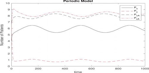
Figure 5. (a) Prevalence of colonized patients with or without antibiotic exposure of model (1(1) $\begin{array}{r}\begin{array}{rl}\frac{\mathrm{d}{P}_u}{\mathrm{d}t}& ={\theta }_u\mathrm{\Omega }\left(t\right)-{\alpha }_p{\beta }_p(1-\eta )P_u{H}_c-{\kappa }_p{P}_u{B}_e-{\gamma }_u{P}_u-ϵ\left(t\right)P_u,\\ \frac{\mathrm{d}{P}_c}{\mathrm{d}t}& ={\theta }_c\mathrm{\Omega }\left(t\right)+{\alpha }_p{\beta }_p(1-\eta )P_u{H}_c+{\kappa }_p{P}_u{B}_e-{\gamma }_c{P}_c-ϵ\left(t\right)P_c,\\ \frac{\mathrm{d}{P}_{uA}}{\mathrm{d}t}& ={\theta }_{uA}\mathrm{\Omega }\left(t\right)-{\alpha }_p{\beta }_{pA}(1-\eta )P_{uA}{H}_c-{\kappa }_{pA}{P}_{uA}{B}_e-{\gamma }_{uA}{P}_{uA}+ϵ\left(t\right)P_u,\\ \frac{\mathrm{d}{P}_{cA}}{\mathrm{d}t}& ={\theta }_{cA}\mathrm{\Omega }\left(t\right)+{\alpha }_p{\beta }_{pA}(1-\eta )P_{uA}{H}_c+{\kappa }_{pA}{P}_{uA}{B}_e-{\gamma }_{cA}{P}_{cA}+ϵ\left(t\right)P_c,\\ \frac{\mathrm{d}{H}_u}{\mathrm{d}t}& =-{\alpha }_p{\beta }_h(1-\eta )P_c{H}_u-{\alpha }_p{\beta }_{hA}(1-\eta )P_{cA}{H}_u-{\kappa }_h{H}_u{B}_e+{\mu }_c{H}_c,\\ \frac{\mathrm{d}{H}_c}{\mathrm{d}t}& ={\alpha }_p{\beta }_h(1-\eta )P_c{H}_u+{\alpha }_p{\beta }_{hA}(1-\eta )P_{cA}{H}_u+{\kappa }_h{H}_u{B}_e-{\mu }_c{H}_c,\\ \frac{\mathrm{d}{B}_e}{\mathrm{d}t}& ={\upsilon }_p{P}_c+{\upsilon }_{pA}{P}_{cA}+{\upsilon }_h{H}_c-{\gamma }_b{B}_e\end{array}\end{array}$(1) ) with initial values $(P_u^0,P_{uA}^0,P_c^0,P_{cA}^0,H_u^0,H_c^0,B_e^0)=(4,6,7,6,17,6,1000)$. Parameters are given in Table 1. Compared with antibiotic prescribing rate and (b) The free-living bacterial load in the environment.

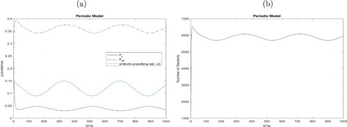
Figure 6. (a) Prevalence of colonized patients with or without antibiotic exposure of the model (1(1) $\begin{array}{r}\begin{array}{rl}\frac{\mathrm{d}{P}_u}{\mathrm{d}t}& ={\theta }_u\mathrm{\Omega }\left(t\right)-{\alpha }_p{\beta }_p(1-\eta )P_u{H}_c-{\kappa }_p{P}_u{B}_e-{\gamma }_u{P}_u-ϵ\left(t\right)P_u,\\ \frac{\mathrm{d}{P}_c}{\mathrm{d}t}& ={\theta }_c\mathrm{\Omega }\left(t\right)+{\alpha }_p{\beta }_p(1-\eta )P_u{H}_c+{\kappa }_p{P}_u{B}_e-{\gamma }_c{P}_c-ϵ\left(t\right)P_c,\\ \frac{\mathrm{d}{P}_{uA}}{\mathrm{d}t}& ={\theta }_{uA}\mathrm{\Omega }\left(t\right)-{\alpha }_p{\beta }_{pA}(1-\eta )P_{uA}{H}_c-{\kappa }_{pA}{P}_{uA}{B}_e-{\gamma }_{uA}{P}_{uA}+ϵ\left(t\right)P_u,\\ \frac{\mathrm{d}{P}_{cA}}{\mathrm{d}t}& ={\theta }_{cA}\mathrm{\Omega }\left(t\right)+{\alpha }_p{\beta }_{pA}(1-\eta )P_{uA}{H}_c+{\kappa }_{pA}{P}_{uA}{B}_e-{\gamma }_{cA}{P}_{cA}+ϵ\left(t\right)P_c,\\ \frac{\mathrm{d}{H}_u}{\mathrm{d}t}& =-{\alpha }_p{\beta }_h(1-\eta )P_c{H}_u-{\alpha }_p{\beta }_{hA}(1-\eta )P_{cA}{H}_u-{\kappa }_h{H}_u{B}_e+{\mu }_c{H}_c,\\ \frac{\mathrm{d}{H}_c}{\mathrm{d}t}& ={\alpha }_p{\beta }_h(1-\eta )P_c{H}_u+{\alpha }_p{\beta }_{hA}(1-\eta )P_{cA}{H}_u+{\kappa }_h{H}_u{B}_e-{\mu }_c{H}_c,\\ \frac{\mathrm{d}{B}_e}{\mathrm{d}t}& ={\upsilon }_p{P}_c+{\upsilon }_{pA}{P}_{cA}+{\upsilon }_h{H}_c-{\gamma }_b{B}_e\end{array}\end{array}$(1) ) with initial values $(P_u^0,P_{uA}^0,P_c^0,P_{cA}^0,H_u^0,H_c^0,B_e^0)=(4,6,7,6,17,6,1000)$, ${\theta }_u=0.62,{\theta }_{uA}=0.38,{\theta }_c=0,{\theta }_{cA}=0$ and other parameter values given in Table 1; (b) The free-living bacterial load in the environment.

Figure 7. (a) Prevalence of colonozied patients with or without antibiotic exposure of modified model (1(1) $\begin{array}{r}\begin{array}{rl}\frac{\mathrm{d}{P}_u}{\mathrm{d}t}& ={\theta }_u\mathrm{\Omega }\left(t\right)-{\alpha }_p{\beta }_p(1-\eta )P_u{H}_c-{\kappa }_p{P}_u{B}_e-{\gamma }_u{P}_u-ϵ\left(t\right)P_u,\\ \frac{\mathrm{d}{P}_c}{\mathrm{d}t}& ={\theta }_c\mathrm{\Omega }\left(t\right)+{\alpha }_p{\beta }_p(1-\eta )P_u{H}_c+{\kappa }_p{P}_u{B}_e-{\gamma }_c{P}_c-ϵ\left(t\right)P_c,\\ \frac{\mathrm{d}{P}_{uA}}{\mathrm{d}t}& ={\theta }_{uA}\mathrm{\Omega }\left(t\right)-{\alpha }_p{\beta }_{pA}(1-\eta )P_{uA}{H}_c-{\kappa }_{pA}{P}_{uA}{B}_e-{\gamma }_{uA}{P}_{uA}+ϵ\left(t\right)P_u,\\ \frac{\mathrm{d}{P}_{cA}}{\mathrm{d}t}& ={\theta }_{cA}\mathrm{\Omega }\left(t\right)+{\alpha }_p{\beta }_{pA}(1-\eta )P_{uA}{H}_c+{\kappa }_{pA}{P}_{uA}{B}_e-{\gamma }_{cA}{P}_{cA}+ϵ\left(t\right)P_c,\\ \frac{\mathrm{d}{H}_u}{\mathrm{d}t}& =-{\alpha }_p{\beta }_h(1-\eta )P_c{H}_u-{\alpha }_p{\beta }_{hA}(1-\eta )P_{cA}{H}_u-{\kappa }_h{H}_u{B}_e+{\mu }_c{H}_c,\\ \frac{\mathrm{d}{H}_c}{\mathrm{d}t}& ={\alpha }_p{\beta }_h(1-\eta )P_c{H}_u+{\alpha }_p{\beta }_{hA}(1-\eta )P_{cA}{H}_u+{\kappa }_h{H}_u{B}_e-{\mu }_c{H}_c,\\ \frac{\mathrm{d}{B}_e}{\mathrm{d}t}& ={\upsilon }_p{P}_c+{\upsilon }_{pA}{P}_{cA}+{\upsilon }_h{H}_c-{\gamma }_b{B}_e\end{array}\end{array}$(1) ) with initial values $(P_u^0,P_{uA}^0,P_c^0,P_{cA}^0,H_u^0,H_c^0,B_e^0)=(4,6,7,6,17,6,1000)$, ${\theta }_u=1,{\theta }_{uA}=0,{\theta }_c=0,{\theta }_{cA}=0$ and other parameter values given in Table 1 and (b) The free-living bacterial load in the environment.

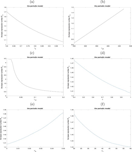
Based on the calculation procedure about the basic reproduction number discussed above, we calculate the basic reproduction number $R_0$ to be 1.476 with the parameter values in Table 1. By Theorem 3.8, we conclude that the infection will persist with the baseline parameter values. In Figure 8, we perform some sensitivity analysis to explore the effect of the following parameters on changing the basic reproduction number $R_0$: (a) The cleaning/disinfection rate of environment ${\gamma }_b$; (b) Shedding rate of bacteria from colonized patients with antibiotic exposure to environment ${\upsilon }_{pA}$; (c) The discharge rate of colonized patients with antibiotic exposure ${\gamma }_{cA}$; (d) The hand hygiene compliance with HCWs η; (e) The contact rate between patients and HCWs ${\alpha }_p$; (f) The decontaminated rate of HCWs ${\mu }_c$. Figure 8(a) shows that increasing the environmental cleaning/disinfection rate ${\gamma }_b$ from 0.6 to 1 can reduce the basic reproduction number from 1.705 to 1.065, which is the most efficient intervention. Since we assume that the free-living bacteria have no proper condition to reproduce themselves, shedding bacteria from colonized patients is a crucial factor in environmental contamination, which is verified in Figure 8(b) where if the shedding rate of colonized patients with antibiotic exposure ${\upsilon }_{pA}$ is below 300, the basic reproduction number can be below 1. This again emphasizes the importance of environmental cleaning. Figure 8(c) indicates that the discharge rate (the inverse of stay in hospital) of colonized patients with antibiotic exposure ${\gamma }_{cA}$ greatly increase the basic reproduction number especially when they have a lengthier stay than 18 days (baseline value i.e. ${0.055}^{-1}$ ). However, it is hard to treat colonized patients with antibiotic exposure efficiently and quickly since they have resistance to many common antibiotics, which usually leads to a lengthier stay to make the situation worse. Hence how to make an efficient and right treatment plan for colonized patients with antibiotic exposure is a challenge and also a key to control the infection. In Figure 8(d), it seems that the hand hygiene compliance of HCWs (from the baseline value 0.4 to 1) make little difference to change the basic reproduction number, which is a little surprising, since the hand hygiene is always thought to be an important intervention. We think that this is because the direct transmission through HCWs is well-known so hospitals have paid enough attention to the hand hygiene of HCWs while the indirect transmission through contaminated environment lacks our surveillance and is more important than we thought. That is why the environmental cleaning ${\gamma }_b$ and the shedding rate ${\gamma }_{cA}$ affect greatly the basic reproduction number in our sensitivity analysis Figure 8(a,b). Hence, we believe that it is necessary to strengthen the surveillance of environmental cleaning with feedback to cleaning team, and try to use more efficient cleaning products. Figure 8(e,f) imply how the contact rate ${\alpha }_p$ and decontaminated rate of HCWs ${\mu }_c$ affect the basic reproduction number.

Figure 8. Effects of parameters on the basic reproduction number $R_0$: (a) ${\gamma }_b$, (b) ${\upsilon }_{pA}$, (c) ${\gamma }_{cA}$, (d) η, (e) ${\alpha }_p$ and (f) ${\mu }_c$. Other parameters values are given in Tabel 1.

5. Discussion

We presented a comprehensive mathematical model with periodic transmission rate to study MRSA infections in hospitals, including key factors such as environmental contamination and antibiotic exposure. Both the direct transmission via HCWs and the indirect transmission via free-living bacteria in the environment were taken into account. Inspired by the work of Sun et al. [22], we modelled the antibiotic prescribing rate as a periodic function depending on time t in the transmission of MRSA, i.e. $ϵ\left(t\right)={ϵ}_0(1+{ϵ}_1\sin (\left(2\pi /365\right)(t-240)\left)\right)$, which has a period of one year (365 days) and implies that antibiotic prescribing rate increases starting at the beginning of August, gains a peak in winter and then decreases starting at the beginning of February according to the data shown in Figures 1 and 2. Based on the definition in Baca$\ddot{e}$r and Guenaoui [2] and the calculation procedure in Wang and Zhao [27], we deduced the basic reproduction number $R_0$ for the periodic deterministic model and carried out some mathematical analysis to prove that the infection would go to extinction if the basic reproduction number is less than unity and would persist if it is greater than unity. On the basis of parameter values given in Table 1, the basic reproduction number is estimated to be $1.476,$ which implies that MRSA infections persist in hospitals. Our simulations suggest that the prevalence of colonized patients with antibiotic exposure has periodic phenomenon between about 34% and 39% and the prevalence of colonized patients without antibiotic exposure is between 4% and 6% in Figures 4 and 5. In addition, since we observe a lag about 15 days between the pattern of colonized patients with antibiotic exposure and antibiotic prescription rate in Figure 5, we suggest that there may be a temporal correlation between antibiotic use and resistance. By controlling the proportion of patients from four compartments on admission, Figures 6 and 7 imply that the prevalence of colonized patients with or without antibiotic exposure would reduce greatly if only uncolonized patients without antibiotic exposure are admitted. This means that detection and isolation of MRSA colonized patients on admission may be a useful intervention to control the hospital infection, and also strengthens the importance to increase the public education about how to use antibiotics properly at community.

It follows from the sensitivity analysis that the basic reproduction number is sensitive to the cleaning/disinfection rate of environment ${\gamma }_b$, shedding rate of bacteria from colonized patients with antibiotic exposure to environment ${\upsilon }_{pA}$, and the discharge rate of colonized patients with antibiotic exposure ${\gamma }_{cA}$. In particular, environmental cleaning is the most important intervention to control the infection according to our sensitivity analysis. Figure 8(a) shows that increasing the environmental cleaning/disinfection rate ${\gamma }_b$ from 0.6 to 1 reduces the basic reproduction number from 1.705 to 1.065. Besides, if the shedding rate of colonized patients with antibiotic exposure ${\upsilon }_{pA}$ is below 300, the basic reproduction number can be below 1 (Figure 8(b)). Because the free-living bacteria have no proper condition to reproduce themselves in hospitals, shedding bacteria from colonized patients becomes a key factor in transmission of MRSA. This also indirectly shows the impact of environmental cleaning. We also found that if colonized patients with antibiotic exposure stay hospitals more than 18 days on average, the basic reproduction number increases dramatically. However, colonized patients with antibiotic exposure usually have resistance to many common antibiotics, which makes it harder and longer to treat them. So how to make an efficient and right treatment plan for colonized patients with antibiotic exposure is a challenge to control the infection. We also observed that the hand hygiene compliance of HCWs change little on the basic reproduction number. We guess the reason is that hospitals have paid enough attention to the hand hygiene of HCWs while still lack attention on the indirect transmission via contaminated environment that maybe is much more important than we thought. This again explains why the environmental cleaning ${\gamma }_b$ and the shedding rate ${\gamma }_{cA}$ affect greatly the basic reproduction number in our sensitivity analysis.

Hence, in order to control the infection, we believe it is necessary to strengthen the surveillance of environmental cleaning with feedback to cleaning team, try to use more efficient cleaning products, highlight the necessary of effective antimicrobial stewardship programmes, increase active screening on admission and subsequent isolation of positive cases, and treat patients quickly and efficiently. Nevertheless, a comprehensive cost-effectiveness analysis of control policy is needed in future work.

Our model emphasizes the importance of incorporating the indirect transmission via free-living bacteria in the environment, where they are assumed to be uniformly distributed. However, bacterial density varies in rooms of hospitals [4], so future work should take the environmental heterogeneity into consideration.

Acknowledgements

We would like to thank the two anonymous reviewers for their helpful comments and suggestions which helped us to improve the paper.

Disclosure statement

No potential conflict of interest was reported by the authors.

Additional information

Funding

This research was partially supported by National Science Foundation ( DMS-1412454) and the University of Miami Provost's Research Award; Directorate for Mathematical and Physical Sciences.

References

- D.J. Austin and R.M. Anderson, Studies of antibiotic resistance within the patient, hospitals and the community using simple mathematical models, Philos. Trans. R. Soc. Lond. B Biol. Sci. 354(1384) (1999), pp. 721–738. doi: 10.1098/rstb.1999.0425
- N. Bacaër and S. Guernaoui, The epidemic threshold of vector-borne diseases with seasonality, J. Math. Biol. 53(3) (2006), pp. 421–436. doi: 10.1007/s00285-006-0015-0
- J.M. Boyce, G. Potter-Bynoe, C. Chenevert and T. King, Environmental contamination due to Methicillin-resistant staphylococcus aureus possible infection control implications, Infect. Control Hosp. Epidemiol. 18(9) (1997), pp. 622–627. doi: 10.1086/502213
- C. Browne and G.F. Webb, A nosocomial epidemic model with infection of patients due to contaminated rooms, Discrete Continuous Dyn. Syst. Ser. B 12 (2015), pp. 761–787.
- Center for Disease Control and Prevention, Antibiotic/antimicrobial Resistance, last updated March 29, 2018. https://www.cdc.gov/drugresistance/index.html.
- F. Chamchod, S. Ruan, Modeling Methicillin-resistant staphylococcus aureus in hospitals: Transmission dynamics, antibiotic usage and its history. Theor. Biol. Med. Model. 9(1) (2012), 25. doi: 10.1186/1742-4682-9-25.
- E.M.C. D'Agata, M.A. Horn, S. Ruan … J.R. Wares, Efficacy of infection control interventions in reducing the spread of multidrug-resistant organisms in the hospital setting. PLoS One 7(2) (2012), e30170. doi: 10.1371/journal.pone.0030170.
- E.M.C. D'Agata, P. Magal, D. Olivier, S. Ruan and G.F. Webb, Modeling antibiotic resistance in hospitals: The impact of minimizing treatment duration, J. Theor. Biol. 249(3) (2007), pp. 487–499. doi: 10.1016/j.jtbi.2007.08.011
- E.M.C D'agata, G.F. Webb, M.A. Horn, R.C. Moellering and S. Ruan, Modeling the invasion of community-acquired Methicillin-resistant staphylococcus aureus into hospitals, Clin. Infect. Dis. 48(3) (2009), pp. 274–284. doi: 10.1086/595844
- S.J. Dancer, How antibiotics can make us sick: The less obvious adverse effects of antimicrobial chemotherapy, Lancet Infect. Dis. 4(10) (2004), pp. 611–619. doi: 10.1016/S1473-3099(04)01145-4
- S.J. Dancer, Importance of the environment in Meticillin-resistant staphylococcus aureus acquisition: The case for hospital cleaning, Lancet Infect. Dis. 8(2) (2008), pp. 101–113. doi: 10.1016/S1473-3099(07)70241-4
- T. Delorme, A. Garcia and P. Nasr, A longitudinal analysis of Methicillin-resistant and sensitive staphylococcus aureus incidence in respect to specimen source, patient location, and temperature variation, Int. J. Infect. Dis. 54 (2017), pp. 50–57. doi: 10.1016/j.ijid.2016.11.405
- T.N. Doan, D.C.M. Kong, C. Marshall, C.M.J. Kirkpatrick and E.S. McBryde, Modeling the impact of interventions against acinetobacter baumannii transmission in intensive care units, Virulence 7(2) (2016), pp. 141–152. doi: 10.1080/21505594.2015.1076615
- M.R. Eber, M. Shardell, M.L. Schweizer … E.N. Perencevich, Seasonal and temperature-associated increases in gram-negative bacterial bloodstream infections among hospitalized patients. PLoS One 6(9) (2011), e25298. doi: 10.1371/journal.pone.0025298.
- J.T. Fishbain, J.C. Lee, H.D. Nguyen, J.A. Mikita, C.P. Mikita, C.F.T Uyehara and D.R. Hospenthal, Nosocomial transmission of Methicillin-resistant staphylococcus aureus: A blinded study to establish baseline acquisition rates, Infect. Control Hosp. Epidemiol. 24(6) (2003), pp. 415–421. doi: 10.1086/502224
- Q. Huang, M.A. Horn and S. Ruan, Modeling the effect of antibiotic exposure on the transmission of Methicillin-resistant staphylococcus aureus in hospitals with environmental contamination. preprint
- S. Leekha, D.J. Diekema and E.N. Perencevich, Seasonality of staphylococcal infections, Clin. Microbiol. Infect. 18(10) (2012), pp. 927–933. doi: 10.1111/j.1469-0691.2012.03955.x
- L.A. Mermel, J.T. Machan, S. Parenteau, Seasonality of MRSA infections. PLoS One 6(3) (2011), e17925. doi: 10.1371/journal.pone.0017925.
- L. Perko, Differential Equations and Dynamical Systems, 3rd ed., Springer, New York, 2000.
- R.E. Polk, C. Fox, A. Mahoney, J. Letcavage and C. MacDougall, Measurement of adult antibacterial drug use in 130 US hospitals: Comparison of defined daily dose and days of therapy, Clin. Infect. Dis.44(5) (2007), pp. 664–670. doi: 10.1086/511640
- R.E. Polk, C.K. Johnson, D. McClish, R.P. Wenzel and M.B. Edmond, Predicting hospital rates of Fluoroquinolone-resistant pseudomonas aeruginosa from fluoroquinolone use in US hospitals and their surrounding communities, Clin. Infect. Dis. 39(4) (2004), pp. 497–503. doi: 10.1086/422647
- L. Sun, E.Y. Klein and R. Laxminarayan, Seasonality and temporal correlation between community antibiotic use and resistance in the United States, Clin. Infect. Dis. 55(5) (2012), pp. 687–694. doi: 10.1093/cid/cis509
- E. Tacconelli, Antimicrobial use: Risk driver of multidrug resistant microorganisms in healthcare settings, Curr. Opin. Infect. Dis. 22(4) (2009), pp. 352–358. doi: 10.1097/QCO.0b013e32832d52e0
- E. Tacconelli, G. De Angelis, M.A. Cataldo, E. Pozzi and R. Cauda, Does antibiotic exposure increase the risk of Methicillin-resistant staphylococcus aureus (MRSA) isolation? A systematic review and meta-analysis, J. Antimicrob. Chemother. 61(1) (2007), pp. 26–38. doi: 10.1093/jac/dkm416
- J. Wang, L. Wang, P. Magal, Y. Wang, S. Zhuo, X. Lu and S. Ruan, Modelling the transmission dynamics of Meticillin-resistant staphylococcus aureus in Beijing Tongren Hospital, J. Hosp. Infect.79(4) (2011), pp. 302–308. doi: 10.1016/j.jhin.2011.08.019
- L. Wang, S. Ruan, Modeling nosocomial infections of Methicillin-resistant staphylococcus aureus with environment contamination. Sci. Rep. 7 (2017), 580. doi: 10.1038/s41598-017-00261-1.
- W. Wang and X.-Q. Zhao, Threshold dynamics for compartmental epidemic models in periodic environments, J. Dyn. Differ. Equ. 20(3) (2008), pp. 699–717. doi: 10.1007/s10884-008-9111-8
- X. Wang, Y. Xiao, J. Wang and X. Lu, A mathematical model of effects of environmental contamination and presence of volunteers on hospital infections in China, J. Theor. Biol. 293 (2012), pp. 161–173. doi: 10.1016/j.jtbi.2011.10.009
- F. Zhang and X.-Q. Zhao, A periodic epidemic model in a patchy environment, J. Math. Anal. Appl.325(1) (2007), pp. 496–516. doi: 10.1016/j.jmaa.2006.01.085
- X.-Q. Zhao, Dynamical Systems in Population Biology, Springer, New York, 2003.