Stochastic differential game for management of non-renewable fishery resource under model ambiguity

ABSTRACT

A new bio-economic model for managing population of non-renewable inland fishery resource in uncertain environment is presented. Population dynamics of the resource is described with stochastic differential equations (SDEs) having ambiguous growth and mortality rates. The performance index to be maximized by the manager of the resource while minimized by nature is presented in the context of differential game theory. The dynamic programming principle leads to a Hamilton–Jacobi–Bellman–Isaacs (HJBI) equation that governs the optimal resource management strategy under the ambiguity. The main contribution of this paper is a series of theoretical analysis on the reduced HJBI equation for non-renewable fishery resources in a broad sense, indicating that the ambiguity critically affects the resulting optimal controls. Practical implications of the theoretical analysis results are also presented focusing on artificially hatched Plecoglossus altivelis (Ayu), an important inland fishery resource in Japan.

KEYWORDS:

• Non-renewable resource
• inland fisheries
• multiplier robust control
• Hamilton–Jacobi–Bellman–Isaacs equation
• Plecoglossus altivelis

CLASSIFICATION CODES:

• 49L20
• 62P20
• 93E20

1. Introduction

Fishery resources in inland waters are of importance from social, economic, ecological, and environmental viewpoints [40], and their sustainable use and conservation have been recent major concerns [12,39]. We are interested in establishment of a sound management strategy for inland fishery resources, which is an urgent problem in the world [6,13,36,57].

Mathematical modelling, especially optimization and optimal control [22,26,66], is a central tool for comprehension and assessment of population dynamics of biological resources from macroscopic viewpoints. Castro-Santis et al. [9] analysed feasibility of regulated fisheries subject to impulsive harvesting strategies. De Zeeuw and He [15] formulated an optimization problem of harvested population subject to catastrophic regime shift. Doyen and Péreau [17] applied static game theory to cooperative management of renewable commons like fishery resources subject to bio-economic constraints. Fenichel and Abbott [19] considered recreational fishing from the standpoint of resource management and analysed feedbacks between policy instruments and angler behaviour. Nowak [53] investigated a multi-generational dynamic game of resource extraction having exact solutions. Stochastic process models have been widely used for describing population dynamics of fishery resources, which are inherently stochastic due to unresolved ecological and environmental processes [31,48,67,76,81,82].

Ambiguity of parameters and coefficients arising from the unresolved processes and/or lack of data is an inevitable issue for identification and operation of a population dynamics model. A possible way for modelling optimal control of population dynamics considering the model ambiguity is to formulate a problem based on the multiplier robust control [23,24]. This mathematical concept handles the model ambiguity in the context of a worst-case, min–max differential game formalism where nature controls the ambiguity. This formalism is based on a penalized performance index to deal with the model ambiguity and has been effectively employed for decision-making problems in economic research areas [21,30,49,53]. The multiplier robust control would potentially serve as a useful mathematical tool for resource management with the potential model ambiguity; however, it has not been applied to management of inland fishery resources so far, which is a strong motivation of our research.

The objectives of this paper are formulation and theoretical analysis of a new bio-economic model for managing non-renewable inland fishery resources, which is a central fisheries problem worldwide including Japan [29,62]. The word ‘non-renewable’ here means that the resource cannot naturally reproduce. Problems of non-renewable fishery resources that the present model may apply to involve aquacultured fishes, and farmed fishes released into natural environment. Some of these resources, even though they are non-renewable, have indispensable economic, ecological, and social roles [2,67,68,75]. Non-renewability of the population distinguishes the present model from the conventional ones for renewable resources. Several researchers have approached optimal management of non-renewable resources from social and economic viewpoints indicating their high importance [3,16,18,35,37,50,63].

The problem focused on in this paper is to find an effective strategy to manage released fish into a river like artificially hatched Plecoglossus altivelis (Ayu) released into rivers in Japan, an important inland fishery resource in the country [62,67,68]. The released P. altivelis can be seen as a non-renewable fishery resource because they are not successful in spawning due to genetic reasons [61]. Nevertheless, this non-renewable inland fishery resource has been a central aquatic species for inland fisheries in Japan [62,67,68]. Therefore, exploring effective management policies of their population is currently an important topic for the inland fishery sector in the country. Our problem has thus fisheries, social, economic, and ecological backgrounds, and relies on a different mathematical formulation based on the multiplier robust control as a new attempt as explained below.

The goal of the present mathematical model is to find the optimal harvesting strategy of a non-renewable fishery resource subject to stochastic population dynamics driven by a Brownian motion and a Lévy process [54], which represent different stochastic fluctuations involved in the dynamics with each other. The population dynamics is also subject to ambiguous mortality and growth rates. The performance index, which is maximized by the manager of the fishery resource while minimized by nature through controlling the ambiguity, is formulated from economic, social and ecological standpoints. Based on the multiplier robust control [24], optimization of the performance index ultimately reduces to solving a terminal and boundary value problem of a Hamilton–Jacobi–Bellman–Isaacs (HJBI) equation. The optimal management strategy under the model ambiguity is derived by solving the HJBI equation. Several differential game problems driven by Lévy processes and the associated HJBI equations have been studied in finance and insurance research areas [14,46,70,80]. The present HJBI equation is exactly solvable under a certain condition where it has a solution of a separation of variables type. The main contribution of this paper is a series of theoretical analysis on the HJBI equation for non-renewable fishery resources in a broad sense. Practical implications of the theoretical analysis results are presented focusing on P. altivelis. Numerical analysis under a more realistic setting is carried out as well. From a standpoint of robust fishery resources management, this paper thus theoretically supports the results that the practitioners have found so far, which have not been achieved in previous studies. This paper can therefore be a first such attempt from a theoretical side to the authors’ knowledge.

The rest of this paper is organized as follows. Section 2 presents the mathematical model used in this paper, and derives the HJBI equation and its reduced counterpart: the main equations. Section 3 performs theoretical analysis on an exactly solvable case where parameter dependence of a solution to the reduced HJBI equation and the associated optimal strategies is tractable. Section 4 focuses on a more realistic case where numerical techniques are required for solving the equation. Section 5 gives conclusions and future perspectives of our research. Appendix A contains the proofs of several propositions in Section 2. Similarly, Appendix B contains the proofs of several propositions in Section 3. Appendix C summarizes theoretical results on a related problem.

2. Mathematical model

The core of the present mathematical model is the HJBI equation, which is derived from a system of stochastic differential equations (SDEs) for population dynamics of a non-renewable fishery resource and a performance index to decide its management strategy. The SDEs, performance index, HJBI equation, and its reduced counterpart are formulated below. Table 1 presents the explanation of the model parameters.

Table 1. Explanation of the model parameters. All the parameters are positive.

Parameter	Explanation
$T$	Terminal time of the problem considered
$R$	Natural mortality rate
$c_{max}$	Maximum harvesting pressure
$\gamma$	Jump intensity
$K$	Maximum body weight of the fish under no noise and ambiguity. This is referred to as the capacity.
$\theta$	Shape parameter of the growth rate $g$
$r$	Intrinsic growth rate of the body weight
$\sigma$	Environmental noise intensity
$\alpha$	Sensitivity constant with $0<\alpha <1$
$w$	Weight parameter for the profit by harvesting
$a$	Weight parameter that quantifies the knowledge of the human on the dynamics of $N_t$
$b$	Weight parameter that quantifies the knowledge of the human on the dynamics of $X_t$

2.1. Stochastic differential equations

Population dynamics of a non-renewable inland fishery resource in a closed habitat is considered. The time is denoted as $t$. The state of the population at $t$ is specified with the total number of population $N_t\left(\ge 0\right)$ in the habitat and their representative body weight $X_t\left(\ge 0\right)$, both of which evolve stochastically in time. Temporal evolution of $N_t$ is assumed to be density-independent, which is valid if there exist not too much individuals in the habitat.

Let $B_t$ with $t\ge 0$ be a standard 1-D Brownian motion on the complete probability space as in the usual setting [54]. Let $Z_t$ with $t\ge 0$ be a subordinator having a mean value with the Lévy’ measure $\nu$, which is a Lévy process having non-negative jumps on the complete probability space [Definition 1.7, of 1]. The simplest example of a subordinator is a standard Poisson process. Mathematical foundation of jump diffusion processes has been well-established [1,54] and is not discussed in detail here, so that this paper does not become too mathematical.

In the present setting, the process $Z_t$ should be a subordinator as assumed above since the population is non-renewable, meaning that $N_t$ decreases with respect to $t$. Since there exist a variety of subordinators [1], the present model would have applicability to wide range of resource management problems. Hereafter, the increment of $Z_t$ is assumed to be in the bounded range $\left(0,{\gamma }^{-1}\right)$, so that $N_t\ge 0$ for $t\ge 0$ almost surely when $N_{-0}\ge 0$ [Chapter 1.5 of 54]. This kind of restriction on the jump intensity exists even for simpler cases to have $N_t\ge 0$ as the analytical examples suggest [Chapter 15 of 56]. The boundedness of the increment of $Z_t$ is necessary to derive the exact solution in Section 3. The process $N_t$ is replaced by 0 once it vanishes ($N_t=0$). The same applies to $X_t$.

We consider a differential game between the two players: the human as the manager of the fishery resource and nature. The present model deals with the situation where the population dynamics is inherently stochastic and the human is aware of it, but the dynamics is subject to ambiguity controlled by nature. The multiplier robust control [24] effectively handles such a situation with a game-theoretic setting.

Assume that the initial condition $\left(N_{-0},X_{-0}\right)$ is given where the notation $\epsilon -0$ represents the left-side limit of $\epsilon \in \mathbb{R}$ and $-0$ for $\epsilon =0$. The governing equations of $N_t$ and $X_t$ for $t\ge 0$ are the jump-diffusion Itô’s SDEs (1) $\text{d}{N}_t=-N_{t-0}\left[\left(R+c_t+{\eta }_t\right)\text{d}t+\gamma \text{d}{Z}_t\right]$(1) and (2) $\text{d}{X}_t=X_t\left[\left(g\left(X_t\right)-{\omega }_t\right)\text{d}t+\sigma \text{d}{B}_t\right],g\left(X_t\right)=r\left(1-{\left(\frac{X_t}{K}\right)}^{\theta }\right),$(2) where $R>0$ is the natural mortality rate, $\sigma >0$ is the environmental noise intensity, $g$ is the growth rate of the generalized logistic type [52,58,59], $r>0$ is the intrinsic growth rate, $K>0$ represents the maximum body weight of the fish under no noise and ambiguity and is hereafter referred to as the capacity, and $\theta >0$ is the shape parameter. The variables $c_t$, ${\eta }_t$, and ${\omega }_t$ for $t\ge 0$ are measurable and adapted variables to be controlled, so that a performance index defined later is optimized. The control variable $c_t$ with the range $\left[0,c_{max}\right]$ is the harvesting pressure from the human to the population where $c_{max}>0$ represents the maximum harvesting pressure. The variables ${\eta }_t$ and ${\omega }_t$ having the range $\mathbb{R}$, which are controlled by nature, represent the model ambiguities involved in the dynamics of $N_t$ and $X_t$, respectively. Unless otherwise specified, the subscript of the control variables is omitted for the sake of simplicity of descriptions. It is shown later that the optimized $\eta$ and $\omega$ are non-negative. The SDE(2) without the model ambiguity has been successfully applied to growth of aquacultured fish in an artificial pool [72,73]. Mean-reverting SDEs like (2), such as the mean-reverting Lévy–Ornstein–Uhlenbeck type [Chapter 1 of 54], have been used in finance. The simpler case $g=r$ is regarded as the limit $\underset{K\to +\mathrm{\infty }}{lim}g=r$. The generalized logistic model serves as a flexible model for growth of organisms. We assume that $\sigma$ is sufficiently small, which is a key to have $X_t\ge 0$ for $t\ge 0$ almost surely when $X_{-0}\ge 0$ [9]. However, this does not provide a sufficient condition to have ‘$X_t\ge 0$ for $t\ge 0$’. The main difficulty is the unboundedness of ${\omega }_t$: if its range is set to be compact, directly following the existing results [Section 3 of 9], we can show $X_t\ge 0$ for $t\ge 0$ almost surely when $X_{-0}\ge 0$. We believe that the fact $\sigma$ is sufficiently small serves as the sufficient condition as well, but its proof can be complicated, which is beyond the scope of this paper. Therefore, hereafter it is assumed that we have $X_t\ge 0$ for $t\ge 0$ almost surely when $X_{-0}\ge 0$. Later, it is demonstrated that the optimized $\omega$ is bounded for some cases, implying that the above-mentioned assumption can be justified. Finally, the term $-\gamma N_{t-0}\text{d}{Z}_t$ with the intensity $\gamma >0$ represents irregular population decrease due to invasions by predators like waterfowls whose dynamics is stochastic [60,67].

2.2. Performance index

The performance index is a utility to be maximized by the human while minimized by nature, which is optimized by the three control variables $c$, $\eta$, and $\omega$. The performance index is formulated so that the utility by the harvesting and the penalization due to the ambiguity are quantified, and the resulting optimization problem can be analysed mathematically under certain additional assumptions. The period considered for managing the fishery resource is $\left[0,T\right)$ with a fixed terminal time $T>0$. The performance index is formulated as (3) $\phi \left(t,n,x;c,\eta ,\omega \right)={\text{E}}^{n,x}\left[{\int }_t^T\frac{{\left(N_s{X}_s\right)}^{1-\alpha }}{1-\alpha }\left(J_1+J_2+J_3\right)\text{d}s\right]$(3) with (4) $J_1=w{c}_s^{1-\alpha },J_2=\frac{a}{2}{\eta }_s^2,\text{and}{J}_3=\frac{b}{2}{\omega }_s^2$(4) where ${\text{E}}^{n,x}$ represents the expectation conditioned on $\left(N_{t-0},X_{t-0}\right)=\left(n,x\right)$ with $n,x\ge 0$, $0<\alpha <1$ is a sensitivity constant, $w$, $a$, and $b$ are positive weight parameters. $\phi$ represents the utility of the human accumulated during the period $\left[t,T\right)$.

Meaning of each term in the right-hand side of (3) is as follows. The first term represents the utility by harvesting the fish, which is assumed to be concave and increasing with respect to the biomass $N_s{X}_s$, having the form of the conventional Constant Relative Risk Aversion (CRRA) utility function widely-used in financial problems [5,38,55]. As in the case of P. altivelis in Japan, the harvested fish would be eaten by anglers, sold in market, or used for ecological education to the residents in some cases [74]. This term therefore evaluates economic, ecological, and social utilities of the harvesting in a lumped manner. The second term represents the penalization due to the ambiguity in the dynamics of $N_t$ following the multiplier robust control approach [23]. The coefficient $a>0$ quantifies the knowledge of the human on the dynamics of $N_t$, and formally larger $a$ represents smaller ambiguity of the dynamics. Similarly, the third term represents the penalization due to the ambiguity in the dynamics of $X_t$. The coefficient $b>0$ quantifies the knowledge of the human on the dynamics of $X_t$ as in the second term. In the present model, $J_2$ and $J_3$ serve as the penalty terms arising from the model ambiguity [24]. They are penalty terms, but we assumed that their magnitudes can be mitigated through improving the knowledge of the decision-maker: namely, through increasing $a$ and $b$. In addition, it is shown that the two terms $J_2$ and $J_3$ actually serve as the penalty to decrease $\phi$ under the present differential game formulation by directly following the equation (14) of Yoshioka and Yaegashi [77]. The coefficient $(1-\alpha {)}^{-1}(N_s{X}_s{)}^{1-\alpha }$ multiplied by the second and third terms, which is increasing with respect to the biomass $N_s{X}_s$, implies that the human has more knowledge on the population dynamics when $N_s{X}_s$ is larger. This functional form of the coefficient is partly for a technical reason to make the reduced HJBI equation, which is presented later, exactly solvable. However, this is a reasonable assumption since the human can less effectively observe the state of the fishery resource when there exists only small biomass. State-dependent coefficients considering problem characteristics as in the present case have been used for the ambiguity penalization [21,41,64].

The value function $\mathrm{\Phi }=\mathrm{\Phi }\left(t,n,x\right)$ is defined as the optimized performance index: (5) $\mathrm{\Phi }=\underset{c}{sup}\underset{\eta ,\omega }{inf}\phi \left(t,n,x;c,\eta ,\omega \right).$(5) This $\mathrm{\Phi }$ is an optimized value of $\phi$ minimized by nature while maximized by the human simultaneously. The optimal $c$, $\eta$, and $\omega$ to give $\mathrm{\Phi }$ are denoted as $c_{}^{\ast }$, ${\eta }_{}^{\ast }$, and ${\omega }_{}^{\ast }$, respectively. By (5), the net utility $P$ obtained during the period $\left[0,T\right)$ subject to the initial condition $\left(N_{-0},X_{-0}\right)=\left(n,x\right)$ is expressed as (6) $P=\mathrm{\Phi }\left(0,n,x\right).$(6) Hereafter in this section, we assume that $N_t$, $X_t$, and $\mathrm{\Phi }$ are sufficiently regular so that the following theoretical analysis is valid. This assumption is satisfied at least for the exactly solvable case in Section 3, and seems to be true for a more realistic case in Section 4.

The value function $\mathrm{\Phi }$ is bounded from below and above since $\mathrm{\Phi }\ge 0$ by its functional form and the inequality (7) $\begin{array}{rl}\mathrm{\Phi }& =\underset{c}{sup}\underset{\eta ,\omega }{inf}\phi \left(t,n,x;c,\eta ,\omega \right)\\ & \le \underset{c}{sup}\phi \left(t,n,x;c,0,0\right)\\ & \le \frac{w{c}_{max}^{1-\alpha }{n}^{1-\alpha }}{1-\alpha }{\text{E}}^{n,x}\left[{\int }_s^T{X_{s,0}}^{1-\alpha }\text{d}s\right]\\ & <+\mathrm{\infty }\end{array}$(7) where $X_{t,0}$ represents the solution to the SDE(2) with ${\omega }_t=0$ ($t\ge 0$). This inequality, especially its first and second lines, means an important fact that the ambiguity always reduces the value function as discussed in Yoshioka and Yaegashi [77] for river environmental management.

The following propositions theoretically characterize dependence of $\mathrm{\Phi }$ on the variables and parameters. We demonstrate that they have clear and intuitive implications. The proofs of Propositions 2.1, 2.2, and 2.3 are presented in Appendix A.

Proposition 2.1

$\mathrm{\Phi }$ is not decreasing with respect to $x\ge 0$ and $n\ge 0$.

Proposition 2.2

$\mathrm{\Phi }$ is not decreasing with respect to $r$ and $K$.

Proposition 2.3

$\mathrm{\Phi }$ is not decreasing with respect to $w$, $a$, and $b$.

Propositions 2.1 means that the net utility is larger for larger available biomass.

Proposition 2.2 shows that the net utility increases as the fishery resource grows better. The human can gain larger utility if the harvesting is more beneficial and he/she has more knowledge about the population dynamics as indicated in Proposition 2.3. The qualitative mathematical analysis results derived in the above-presented propositions can be interpreted as that releasing a larger amount of fish with better quality results in higher profit, which are intuitively reasonable results, and will be quantified later. The most important results of the propositions, which cannot be derived from a model without ambiguity, is that the ambiguity should be made small to achieve successful management of the fish (Proposition 2.3). This implies that, if it is not so costly, then the decision-maker should try to identify the model more accurately so that he/she can employ large $a$ and $b$. If such a trial is costly, then the performance index would have a term on the learning cost as in the literature on stochastic controls under incomplete information [49,39].

For the two terminal times $T_1\le T_2$, by (3), we have ${\phi }_{T=T_1}\le {\phi }_{T=T_2}$ for $0\le t\le min\left\{T_1,T_2\right\}$. Furthermore, by the time-homogeneity of the SDEs (1)-(2), we have ${\phi }_{t=t_1}\ge {\phi }_{t=t_2}$ for $0\le t_1\le t_2\le T$. These observations directly lead to the following proposition, which state that $\mathrm{\Phi }$ is larger for a larger period of harvesting.

Proposition 2.4

$\mathrm{\Phi }$ is not decreasing and not increasing with respect to $T$ and $t$ ($0\le t<T$).

Remark 2.1

Statements of Propositions 2.1 through 2.3 also hold when the coefficient $(1-\alpha {)}^{-1}(N_s{X}_s{)}^{1-\alpha }$ is replaced by a sufficiently regular function $h=h\left(N_s,X_s\right)$ that is increasing with respect to the first and second arguments if $\mathrm{\Phi }$ remains bounded. Therefore, Propositions 2.1 through 2.3 hold for wider class of the functional forms of the performance index. In addition, Propositions 2.1 and 2.4 imply $\frac{\mathrm{\partial \Phi }}{\mathrm{\partial }x}\ge 0$, $\frac{\mathrm{\partial \Phi }}{\mathrm{\partial }n}\ge 0$, and $\frac{\mathrm{\partial \Phi }}{\mathrm{\partial }t}\le 0$ if $\mathrm{\Phi }$ is partially differentiable with respect to the independent variables.

Remark 2.2

A remark on economic aspects of the present mathematical model are presented based on the results obtained in this section. Firstly, the boundedness of the value function $\mathrm{\Phi }$ in (7) seems to be somewhat not intuitive since it means that $\mathrm{\Phi }$ is bounded for arbitrary and possibly unbounded $T$ even if there exists no explicit discount factor as in the standard optimal control models [8,25,34]. This property distinguishes the present model for management of non-renewable resources from the existing ones for renewable ones. The reason of this property of the present model lies in the fact that the governing equation of $N_t$ is that of a death process, and the factor $N_s^{1-\alpha }$ implicitly serves as a time-inhomogeneous discount factor [42,43]. This implies an economic linkage between the present and existing models that the problem for non-renewable fishery resources can be formally seen as a discounted problem for renewable resources.

2.3. Hamilton–Jacobi–Bellman–Isaacs (HJBI) equation

The HJBI equation governs evolution of the value function $\mathrm{\Phi }$. The domain of $\mathrm{\Phi }$ is $\left(t,n,x\right)\text{ with }n>0,x>0,0\le t<T$. Hereafter, the parameter value $w=1$ has been specified without any loss of generality of analysis. This is because what is important here is not the values of the weights $w$, $a$, and $b$, but the ratios $a{w}^{-1}$ and $b{w}^{-1}$. Therefore, setting $w=1$ does not critically affect the model structure and the analysis results of this paper.

Straightforward calculation with the application of the dynamic programming principle [24,54] to (5) formally leads to the HJBI equation (8) $-\frac{\mathrm{\partial \Phi }}{\mathrm{\partial }t}+\underset{c\in \left[0,c_{max}\right]}{min}\underset{\eta ,\omega \in \mathbb{R}}{max}{L}_{c,\eta ,\omega }\mathrm{\Phi }=0,n>0,x>0,0\le t<T$(8) with the degenerate elliptic partial integro-differential operator $L_{c,\eta ,\omega }$ defined for generic sufficiently regular $f=f\left(t,n,x\right)$ as (9) $\begin{array}{rl}{L}_{c,\eta ,\omega }f& =\left(R+c+\eta \right)n\frac{\mathrm{\partial }f}{\mathrm{\partial }n}+\left(\omega -g\left(x\right)\right)x\frac{\mathrm{\partial }f}{\mathrm{\partial }x}-\frac{{\sigma }^2{x}^2}{2}\frac{{\mathrm{\partial }}^{2}f}{\mathrm{\partial }{x}^2}\\ & -{\int }_0^{{\gamma }^{-1}}\left[f\left(t,n\left(1-\gamma y\right),x\right)-f\left(t,n,x\right)\right]\nu \left(\text{d}y\right)\\ & -\frac{{\left(nx\right)}^{1-\alpha }}{1-\alpha }\left(c^{1-\alpha }+\frac{a}{2}{\eta }^2+\frac{b}{2}{\omega }^2\right).\end{array}$(9)

The HJBI equation (8) is subject to the terminal and boundary conditions (10) $\mathrm{\Phi }=0\text{for}nx\left(T-t\right)=0.$(10) Since the ‘max’ and ‘min’ terms in (8) are separable with each other, following the standard approach to obtain optimal controls [24,54], the optimal controls $c^{\ast }$, ${\eta }^{\ast }$, and ${\omega }^{\ast }$ to be chosen for each state $\left(t,n,x\right)$ are analytically expressed with $\mathrm{\Phi }$ and its partial derivatives as (11) $c^{\ast }=min\left\{c_{max},{\left(\frac{{\left(nx\right)}^{1-\alpha }}{n}{\left(\frac{\mathrm{\partial \Phi }}{\mathrm{\partial }n}\right)}^{-1}\right)}^{-1/\alpha }\right\},{\eta }^{\ast }=\frac{\left(1-\alpha \right)x}{a{\left(nx\right)}^{1-\alpha }}\frac{\mathrm{\partial \Phi }}{\mathrm{\partial }x},{\omega }^{\ast }=\frac{\left(1-\alpha \right)n}{b{\left(nx\right)}^{1-\alpha }}\frac{\mathrm{\partial \Phi }}{\mathrm{\partial }n}.$(11) Thus, finding the optimal controls reduces to solving the HJBI equation (8). In (11), we assumed that $\frac{\mathrm{\partial \Phi }}{\mathrm{\partial }n}$ is not negative by Proposition 2.1.

2.4. Reduced HJBI equation

The reduced HJBI equation that governs a solution of the HJBI equation of a separation of variables type is derived. Based on the functional form of $\phi$ in (3), we examine the functional form of the value function (12) $\mathrm{\Phi }\left(t,n,x\right)=\frac{n^{1-\alpha }}{1-\alpha }\mathrm{\Psi }\left(t,x\right)$(12) with a bi-variate function $\mathrm{\Psi }=\mathrm{\Psi }\left(t,x\right)$. This ansatz is based on the functional form of the performance index $\phi$ and the linearity of the SDE (1) with respect to $N_t$. The domain of $\mathrm{\Psi }$ is$\left(t,x\right)\text{ with }x>0,0\le t<T$. Substituting (12) into (8) yields the reduced HJBI equation (13) $-\frac{\mathrm{\partial \Psi }}{\mathrm{\partial }t}+\underset{c\in \left[0,c_{max}\right]}{min}\underset{\eta ,\omega \in \mathbb{R}}{max}{\hat{L}}_{c,\eta ,\omega }\mathrm{\Psi }=0,x>0,0\le t<T$(13) with the degenerate elliptic operator ${\hat{L}}_{c,\eta ,\omega }$ defined for generic sufficiently regular $f=f\left(t,x\right)$ as (14) $\begin{array}{rl}{\hat{L}}_{c,\eta ,\omega }f& =\left[\left(1-\alpha \right)\left(R+c+\eta \right)+\lambda \right]f+\left(\omega -g\left(x\right)\right)x\frac{\mathrm{\partial }f}{\mathrm{\partial }x}-\frac{{\sigma }^2{x}^2}{2}\frac{{\mathrm{\partial }}^{2}f}{\mathrm{\partial }{x}^2}\\ & -x^{1-\alpha }\left(c^{1-\alpha }+\frac{a}{2}{\eta }^2+\frac{b}{2}{\omega }^2\right)\end{array}$(14) with (15) $\lambda =-{\int }_0^{{\gamma }^{-1}}\left[{\left(1-\gamma y\right)}^{1-\alpha }-1\right]\nu \left(\text{d}y\right)>0.$(15) The quantity $-\left[{\left(1-\gamma y\right)}^{1-\alpha }-1\right]$ in (15) is non-negative and increasing with respect to $\gamma >0$ for $0\le y\le {\gamma }^{-1}$. The reduced HJBI equation (14) is subject to the terminal and boundary conditions (16) $\mathrm{\Psi }=0\text{for}x\left(T-t\right)=0,$(16) which are compatible with (10). By (11), the optimal controls $c^{\ast }$, ${\eta }^{\ast }$, and ${\omega }^{\ast }$ to be chosen for the state $\left(t,x\right)$ are expressed with $\mathrm{\Psi }$ as (17) $c^{\ast }=min\left\{c_{max},{\left(\frac{x^{1-\alpha }}{\mathrm{\Psi }}\right)}^{-1/\alpha }\right\},{\eta }^{\ast }=\frac{1}{a}{x}^{\alpha }\frac{\mathrm{\partial \Psi }}{\mathrm{\partial }x},{\omega }^{\ast }=\frac{1-\alpha }{b}\frac{\mathrm{\Psi }}{x^{1-\alpha }}.$(17)

Remark 2.3

The optimal controls $c^{\ast }$, ${\eta }^{\ast }$, and ${\omega }^{\ast }$ are independent from $n$ by (17) due to the assumption of the density independent population dynamics. In addition, Proposition 2.1 at least formally leads to that $c^{\ast }$, ${\eta }^{\ast }$, and ${\omega }^{\ast }$ are non-negative.

Remark 2.4

The HJBI equation (9) is a parabolic partial integro-differential equation, while the reduced counterpart (14) is a parabolic partial differential equation more convenient to handle both from mathematical and numerical viewpoints. This is a technical advantage of considering the present functional forms of the population dynamics model and the performance index.

Remark 2.5

The main difference between the present model and that of Yaegashi et al. [69] is that the former considers the model ambiguity and jump, while the latter does not. Therefore, the model of Yaegashi et al. [69] assumes that it has no ambiguity and no jump, which thus deals with a more restricted problem than that in this paper. In addition, although it may be a technical difference, the present mathematical model is at least partly tractable and its properties can be analysed exactly by the mathematical analysis carried out later. On the other hand, for the latter model, due to its model complexity, the behaviour of the value function and the optimal controls are analysed solely from numerical viewpoints. Mathematically exact and explicit results, even if they are somewhat idealized, can effectively characterize the fishery resource dynamics and its optimal management policy as the previous studies on the resources management show [11,45,65].

Remark 2.6

Although this paper focuses on fishery resources management in rivers under ambiguity, the present framework of mathematical modelling can also be applied to effectively handling problems in aquaculture systems [7,32,73,78], in which the population dynamics is seen as non-renewable. Robust management of the aquacultured fishery resources can be analysed by considering ambiguities of the body growth rate and the decrease of the population.

3. Theoretical analysis

An exactly solvable case of the reduced HJBI equation (13) is theoretically analysed in this section from a broad sense, and its practical implications are discussed focusing on P. altivelis in Japan. The problem discussed here is simpler than that dealt with numerically in the next section, but has clear practical implications.

3.1. Mathematical analysis results

The authors carried out interviews to officers of Hii River Fisheries Cooperatives, San-in area, Japan (December 15, 2017 at their office). The officers said that ‘We put importance on managing the predation from the waterfowl such as a cormorant to P. altivelis and riverbed conditions of the habitat of P. altivelis in Hii River.’ They also said that ‘We want to evaluate their effects on the population dynamics of P. altivelis’. In the context of the present model, this means that they put importance on the parameters $r$, $R$, and $\gamma$. Analysing their influences on the value function and the resulting optimal controls can show how they should manage the fishery resources under various conditions. This motivates the following sensitivity analysis of the present model on its parameters.

In this section, we assume $g=r>0$, meaning that the growth of the fishery resource is governed by an SDE of a Geometric Brownian type. The assumption of the constant growth rate $g=r$ leads to more optimistic results than the generalized logistic model in (2) since the growth with the former is not limited by the capacity $K$; namely, $rx\left(1-{\left(x/K\right)}^{\theta }\right)$ for $x>0$ is increasing with respect to $K$. We also assume that most of the population is out of the system by the terminal time $t=T$ due to harvesting, natural death, or predation. This assumption allows us to consider the limit $T\to +\mathrm{\infty }$. Then, the problem is formulated in an infinite time horizon where the terminal condition is not required and the first term of (13) is dropped. The present exact solution is useful for comprehension of behaviour of the value function and optimal controls because their parameter dependence is clearly evaluated.

We guess the solution to the reduced HJBI equation (13) having the form (18) $\mathrm{\Psi }=x^{1-\alpha }\hat{z}$(18) with a constant $\hat{z}>0$. The ansatz is based on the functional form of the performance index $\phi$ and the formal linearity of the SDE (2) ($g=r$) with respect to $X_t$. Under the stated assumptions, substituting (18) into (13) shows that the solution of the form (18) exists and is unique if $z=\hat{z}>0$ solves (19) $A{z}^2-{\hat{c}}^{1-\alpha }+\left(1-\alpha \right)\hat{c}z-Bz=0,\hat{c}=\hat{c}\left(z\right)=min\left\{c_{max},z^{-1/\alpha }\right\}$(19) with (20) $A=\frac{{\left(1-\alpha \right)}^2}{2}\left(\frac{1}{a}+\frac{1}{b}\right)>0\text{and }B=\left(1-\alpha \right)\left(r-R-\frac{\alpha {\sigma }^2}{2}\right)-\lambda .$(20) By (17), the optimal controls are expressed with $\hat{z}$ as (21) $c^{\ast }=\hat{c},{\eta }^{\ast }=\frac{1-\alpha }{a}\hat{z},{\omega }^{\ast }=\frac{1-\alpha }{b}\hat{z},$(21) which are now positive constants.

The following propositions hold for the equation (19). Proofs of the Propositions 3.1, 3.3, and 3.4 are provided in Appendix B. The proof of Proposition 3.2 is not provided since it can be checked by direct substitutions. Theoretical results for a problem with the discount are presented in Appendix C. It should be noted that the following propositions are universally valid for $0<\alpha <1$. In this paper, a classical solution is a solution to (8) or (13) that is continuously differentiable with respect to $t$ and twice continuously differentiable with respect to $x$.

Proposition 3.1

There exists a unique $z=\hat{z}>0$ that solves (19).

Proposition 3.2

$\mathrm{\Psi }$ in (18) is a time-independent classical solution to (13) that satisfies the boundary condition. In addition, $\mathrm{\Phi }$ with this $\mathrm{\Psi }$ is a time-independent classical solution to (8) that satisfies the boundary condition.

Remark 3.1

The existence of the second and third terms in (3) on the penalization is indispensable to have the non-trivial solution. Without this term ($a=b=0$), the equation (19) reduces to (22) $-{\hat{c}}^{1-\alpha }+\left(1-\alpha \right)\hat{c}z-Bz=0,$(22) which does not have positive solutions when $B\ge 0$.

Remark 3.2

$\mathrm{\Psi }$ in (18) is actually a time-independent continuous viscosity solution [Definition 4.2 of 20] to (13) that satisfies the boundary condition as well. Here, a viscosity solution is a ‘weak’ solution to (13) that may not be defined in the classical sense but complies with certain inequalities [20]. Since a classical solution is always a viscosity solution, the first sentence of this Remark seems to be trivial. However, this is an important result that characterizes the derived solution since solutions to elliptic and parabolic equations arising in stochastic control and differential game problems have been discussed from the view point of viscosity solutions.

Analysis of $\mathrm{\Psi }$ in (18) thus reduces to analysis of the parameter dependence of the coefficient $\hat{z}$. The following proposition holds for the coefficient $\hat{z}$ as a function of the parameters.

Proposition 3.3

$\frac{\mathrm{\partial }\hat{z}}{\mathrm{\partial }r},-\frac{\mathrm{\partial }\hat{z}}{\mathrm{\partial }R},-\frac{\mathrm{\partial }\hat{z}}{\mathrm{\partial }\gamma },-\frac{\mathrm{\partial }\hat{z}}{\mathrm{\partial }\left({\sigma }^2\right)},\frac{\mathrm{\partial }\hat{z}}{\mathrm{\partial }a},\frac{\mathrm{\partial }\hat{z}}{\mathrm{\partial }b}>0.$

Remark 3.3

Proposition 3.3 complies with Propositions 2.1 through 2.3.

Proposition 3.3 leads to the following key proposition on the optimal controls.

Proposition 3.4

$\frac{\mathrm{\partial }\mu }{\mathrm{\partial }r},-\frac{\mathrm{\partial }\mu }{\mathrm{\partial }R},-\frac{\mathrm{\partial }\mu }{\mathrm{\partial }\gamma },-\frac{\mathrm{\partial }\mu }{\mathrm{\partial }\left({\sigma }^2\right)},-\frac{\mathrm{\partial }\mu }{\mathrm{\partial }a},-\frac{\mathrm{\partial }\mu }{\mathrm{\partial }b}>0$ where $\mu$ represents ${\eta }^{\ast }$ or ${\omega }^{\ast }$. In addition, these inequalities hold for $-c^{\ast }$ when ‘$>$’ is replaced by ‘$\ge$’.

The following proposition characterizes parameter dependence of $\hat{z}$, the value function, and the optimal controls on the maximum harvesting pressure $c_{max}$.

Proposition 3.5

Let $\mu$ represent $-c^{\ast }$, ${\eta }^{\ast }$, or ${\omega }^{\ast }$. Assume $\hat{z}\ge c_{max}^{-\alpha }$. Then, $\frac{\mathrm{\partial }\hat{z}}{\mathrm{\partial }{c}_{max}}=0$ and $\frac{\mathrm{\partial }\mu }{\mathrm{\partial }{c}_{max}}=0$. On the other hand, assume $\hat{z}<c_{max}^{-\alpha }$. Then, $\frac{\mathrm{\partial }\hat{z}}{\mathrm{\partial }{c}_{max}}>0$ and $\frac{\mathrm{\partial }\mu }{\mathrm{\partial }{c}_{max}}>0$.

Proof of Proposition 3.5 is essentially the same with that of Proposition 3.4, and is therefore not presented.

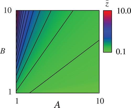
Figure 1 presents $\hat{z}$ for $\alpha =0.5$ as a function of $A$ and $B$ where $c_{max}$ is replaced by 1 without any loss of generality. This treatment corresponds to the following non-dimensionalization: $A\to A{c}_{max}^{1+\alpha }$, $B\to B{c}_{max}^{}$, $z\to z{c}_{max}^{-\alpha }$. Figure 1 actually contains dependence of $\hat{z}$ on each model parameter, since $A$ and $B$ are monotone functions of the model parameters as shown in (20). In addition, (21) presents explicit linkages among the optimal controls, model parameters, and $\hat{z}$. Therefore, this figure can be useful for graphically understanding the theoretical results. Figure 1 verifies the monotone dependence of $\hat{z}$ on the model parameters as indicated in Propositions 3.3 through 3.5, and Appendix B. The behaviour of $\hat{z}$ for other values of $0<\alpha <1$ has been checked to be qualitatively the same.

Figure 1. Dependence of $\hat{z}$ on $A$ and $B$.

3.2. Practical implications

Implications of the theoretical analysis results for the exactly solvable case from practical viewpoints are presented focusing on the artificially hatched P. altivelis in Japan, which is one of the most economically and culturally important inland fishery resources in the country. The explanation on the life history of the fish follows that of Yaegashi et al. [68]. The adult fishes spawn during autumn in downstream reaches of a river, and die afterwards. Hatched larvae descend to the downstream coastal areas, which is the sea or an estuary. They ascend into the midstream of the river in the coming spring until the next autumn to mature. The life history of artificially hatched P. altivelis is somewhat different from that of the natural one [29,62,67]. They are grown up in breeding facilities during winter, and released into a river in the coming spring by inland fishery cooperatives. The artificially hatched P. altivelis is thought to be non-renewable because they are unsuccessful in reproduction due to genetic issues [61].

Propositions 3.3 and 3.4 have significant importance for management of non-renewable fishery resources including the artificially hatched P. altivelis. Proposition 3.3 reveals dependence of $\hat{z}$, which is equivalent to the net utility for given $\left(n,x\right)$, on the environmental and ecological conditions. From Proposition 3.3, we see that $\hat{z}$ is larger for the larger growth rate, smaller mortality rate, smaller predation pressure, or smaller stochastic fluctuation of the growth. $\hat{z}$ is larger if the human has more knowledge on the population dynamics as well. In the real-world context focusing on P. altivelis, the above theoretical results indicate that the human can potentially gain larger utility when the following conditions are realized; there exist much diatoms, the staple food of the fish in the habitat. Predation by the waterfowls [47] and invasive fishes [10] should be suppressed to reduce the predation pressure, so that the net utility potentially increases. River water quality, such as water temperature and suspended sediment concentration, should be kept within appropriate ranges, outside which the mortality rate of the fish significantly increases [27,51]. Proposition 3.4, the statement on the key parameters $a$ and $b$, shows that the resulting ambiguities are smaller and the optimal harvesting pressure is larger if the human has more knowledge on the population dynamics of the fish. This theoretical result indicates the critical importance to have an accurate estimate on the population dynamics for the fisheries management. For example, regular monitoring, if it is simple and not costly, of river environment and ecology would be helpful for accumulating the knowledge on the fish population dynamics.

Proposition 3.5 shows that the optimal controls and the value function do not explicitly depend on $c_{max}$ if it is sufficiently large. This condition is satisfied when the model ambiguity, which is modulated by the parameters $a^{-1}$ and $b^{-1}$, is sufficiently small by (A7) of Appendix B. Otherwise, harvesting the fish with the maximum harvesting pressure $c_{max}$ results in optimal. Proposition 3.5 thus implies that to have sufficient knowledge on the population dynamics is crucial for their management with a not maximum level of the harvesting pressure.

Comparisons between the obtained results and the existing ones are briefly carried out. To the authors’ knowledge, similar problems (robust optimal control of the population of P. altivelis) to ours have not been addressed so far. There exist similar models without ambiguity, which are presented in Yaegashi et al. [68] and Yoshioka and Yaegashi [75]. These models do not have jumps in the population dynamics. The short paper Yoshioka and Yaegashi [75] discussed a deterministic variant of the present model without model ambiguity, carried out its qualitative mathematical analysis. This paper concluded that managing river environment with less predation and much staple food is essential for current inland fishery resources, especially P. altivelis. This is qualitatively consistent with the present mathematical analysis results. In addition, Yaegashi et al. [68], although not mathematically but numerically, carried out sensitivity analysis of a value function and statistical indices for assessing the performance of the management policy of the released P. altivelis. They reported qualitatively the same results with those stated in Proposition 3.3 on the parameters $R$, $\gamma$, and $\sigma$ from a standpoint of the present model. The above-mentioned previous papers did not simultaneously address qualitative analysis and numerical analysis, while the present mathematical analysis is both qualitative and quantitative since it is exactly solvable, and at least partly supports their results theoretically. Although not a research on fishery management, Evatt et al. [18] numerically showed for a non-renewable resource extraction problem that increasing the parameter $\sigma$ results in a decreased total profit as in Proposition 3.3. The computational results presented in the next section quantify the fishery resources management under different environmental conditions.

4. Numerical analysis

The reduced HJBI equation (13) is numerically solved to analyse the problem under a more realistic condition.

4.1. Computational method

The reduced HJBI(13) is a degenerate parabolic partial differential equation whose form is suited to numerically solve with the 1-D Petrov-Galerkin finite element scheme [71]. The scheme can handle degenerate parabolic equations in a stable manner, and has been successfully applied to degenerate parabolic partial differential equations such as Hamilton–Jacobi–Bellman equations arising in ecological and fisheries problems [67,68,73,76]. The true spatial domain $\left(0,+\mathrm{\infty }\right)$ to define the reduced HJBI(13) is unbounded, but is truncated as $\left(0,X_{max}\right)$ with a sufficiently positive large number $X_{max}>K$ where the homogenous Neumann condition ${\left.\frac{\mathrm{\partial \Psi }}{\mathrm{\partial }x}\right|}_{x=X_{max}}=0$ is specified, since practical interest would be in and near the sub-domain $\left(0,K\right)$. Therefore, this paper employs the value $X_{max}=4K$ in what follows, which was preliminary found to be sufficiently large for approximating solutions in and near $\left(0,K\right)$. A similar numerical treatment has already been employed in Yoshioka and Yaegashi [73]. The computational domain is uniformly discretized into 800 and 24,000 intervals, which is found to be sufficiently fine resolution for approximating solutions to the reduced HJBI equation. The equation is integrated backward in time with the terminal and boundary conditions directly specified.

4.2. Computational conditions

The model parameters are estimated from the previous research results on the artificially hatched P. altivelis released into Hii River, Japan [67,68]. The growth of the fish has been successfully modelled with the conventional logistic model $g\left(X_t\right)=r\left(1-X_t/K\right)$ ($\theta =1$) [72,73]. The process $Z_t$ is assumed to be a standard Poisson process with $\lambda =1.0\times {10}^{-2}$ (1/day) for the sake of simplicity of analysis, which corresponds to the same level of predation that is considered in Yaegashi et al. [67,68]. P. altivelis is introduced into Hii River in each May. Since the period allowed to harvest the fish in Hii River starts at the beginning of July and most of the fish population disappears from the river at the end of coming October, $T=120$ (day) is specified. Table 2 provides the above-presented and the other nominal model parameter values. The nominal values of the parameters $a$ and $b$, which do not appear in Yaegashi et al. [68], have been specified so that the magnitudes of the resulting ${\eta }^{\ast }$ and ${\omega }^{\ast }$ are less than or equal to those of $c_{max}$ and $r$. $\alpha$ is set as 0.5.

Table 2. Specified model parameter values.

Parameter	Nominal value	Non-dimensionalized value
$T$	120 (day)	1
$K$	$5.1\times {10}^{-2}$ (g)	1
$R$	$3.9\times {10}^{-3}$ (1/day)	$4.7\times {10}^{-1}$
$r$	$7.1\times {10}^{-2}$ (1/day)	$8.5\times {10}^0$
$c_{max}$	$1.0\times {10}^{-2}$ (1/day)	$1.2\times {10}^0$
$\lambda$	$5.0\times {10}^{-3}$ (1/day)	$6.0\times {10}^{-1}$
$\sigma$	$1.0\times {10}^{-1}$ (1/day^1/2)	$1.1\times {10}^1$
$a$	500 (day^3/2)	$3.8\times {10}^{-1}$
$b$	500 (day^3/2)	$3.8\times {10}^{-1}$

For the sake of brevity of descriptions, the following non-dimensionalization is employed in what follows: $t{T}^{-1}\to t$, $x{K}^{-1}\to x$, $\mu T\to \mu$ where $\mu$ represents $R$, $r$, ${\sigma }^2$, $\lambda$, $c_{max}$, or $c$, $a{T}^{1+\alpha }\to a$, $b{T}^{1+\alpha }\to b$, and $K^{\alpha -1}{T}^{-\alpha }\mathrm{\Psi }\to \mathrm{\Psi }$. The reduced HJBI equation (14) is now written with the non-dimensional variables and parameters as (23) $-\frac{\mathrm{\partial \Psi }}{\mathrm{\partial }t}+\underset{c\in \left[0,1\right]}{min}\underset{\eta ,\omega \in \mathbb{R}}{max}{\hat{L}}_{c,\eta ,\omega }\mathrm{\Psi }=0,$(23) where (24) $\begin{array}{rl}{\hat{L}}_{c,\eta ,\omega }\mathrm{\Psi }& =\left(D+c+\eta \right)\mathrm{\Psi }+\left(\omega -r\left(1-x\right)\right)x\frac{\mathrm{\partial \Psi }}{\mathrm{\partial }x}-\frac{{\sigma }^2{x}^2}{2}\frac{{\mathrm{\partial }}^2\mathrm{\Psi }}{\mathrm{\partial }{x}^2}\\ & -x^{1-\alpha }\left(c^{1-\alpha }+\frac{a}{2}{\eta }^2+\frac{b}{2}{\omega }^2\right)\end{array}$(24) with $D=\left(1-\alpha \right)R+\lambda$, demonstrating that the effective non-dimensional model parameters are $D$, $\sigma$, $r$, $a$, and $b$.

4.3. Computational results

Figures 2–5 show the computed $\mathrm{\Psi }$ and the optimal controls $c^{\ast }$, ${\eta }^{\ast }$, and ${\omega }^{\ast }$ for the nominal parameter values in Table 2. Figure 2 shows that the computed $\mathrm{\Psi }$ is increasing and decreasing with respect to $x$ and $t$, respectively, as theoretically indicated in Propositions 2.1 and 2.4. In addition, the computed $\mathrm{\Psi }$ seems to be concave with respect to $x$ as in the exactly solvable case. The concavity of $\mathrm{\Psi }$, however, is not a trivial fact due to the not simple functional shape of the objective function and the nonlinearity of the drift term of the SDE(2). Figure 3 shows that the optimal $c^{\ast }$ is increasing with respect to $x$ and implies that the harvesting should not be performed at the maximum rate when they do not sufficiently grow up except for the period near the terminal time $t=1$. This result means that it is more beneficial not to harvest the fish with small body weight near the initial time because the fish would have enough time to grow up during the period considered. Figures 4 and 5 show that the resulting ${\eta }^{\ast }$ and ${\omega }^{\ast }$ are smaller for better-grown fish. The computational results presented in Figures 4 and 5 indicate that ${\eta }^{\ast }$ and ${\omega }^{\ast }$ for each $x$ are decreasing with respect to $t$, meaning that the model ambiguity decreases as the time elapses. This is in accordance with the intuition that the knowledge about the population dynamics would increase as the time elapses and as the fish grows up. Figures 4 and 5 also indicate that ${\eta }^{\ast }$ and ${\omega }^{\ast }$ are significantly large for small $x$ and $t$, implying huge ambiguity is involved in the population dynamics. The result recommends to grow up the fish well especially at the beginning of the period. It should be noted that state-dependence of the optimal controls $c^{\ast }$, ${\eta }^{\ast }$, and ${\omega }^{\ast }$, as in the present case, does not result from the exactly solvable case that deals with a simpler situation with the constant growth rate $g=r$. In addition, the computational results demonstrate that the present finite element scheme can handle the reduced HJBI equation in a stable manner since the numerical solutions do not have spurious oscillations.

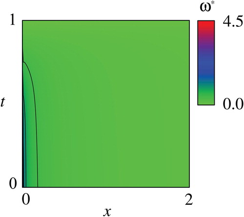
Figure 2. Computed value function $\mathrm{\Phi }$ with the parameter values in Table 2.

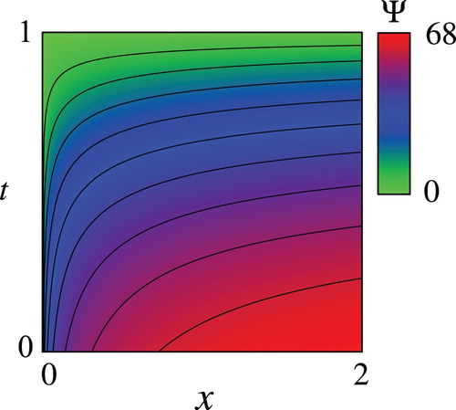
Figure 3. Computed optimal control $c^{\ast }$ with the parameter values in Table 2.

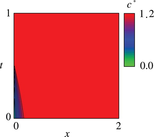
Figure 4. Computed optimal control ${\eta }^{\ast }$ with the parameter values in Table 2.

Figure 5. Computed optimal control ${\omega }^{\ast }$ with the parameter values in Table 2.

The quantity $\mathrm{\Psi }\left(0,x\right)$, which has a similar meaning with the net utility $P$ since $P=(1-\alpha {)}^{-1}{n}^{1-\alpha }\mathrm{\Psi }\left(0,x\right)$, is computed to see its dependence on the non-dimensional parameters $D$, $\sigma$, $r$, $a$, and $b$. The notation $\mathrm{\Psi }=\mathrm{\Psi }\left(0,x\right)$ is utilized for the sake of simplicity of descriptions in what follows. Figures 6 through 10 plot the computed $\mathrm{\Psi }$ for different values of the non-dimensional parameters $D$, $\sigma$, $r$, $a$, and $b$. Figures 6 and 7 show that $\mathrm{\Psi }$ decreases as $D$ increases or $\sigma$ increases, and Figures 8–10 indicate that $\mathrm{\Psi }$ increases as $r$, $a$ or $b$ increases. Figures 9 and 10 further imply that the impacts of the parameters $a$ and $b$ on $\mathrm{\Psi }$ are not significant and reach a plateau curve when they are sufficiently large ($a,b\to +\mathrm{\infty }$). Therefore, the results recommend that the human should try to reduce the mortality and increase the growth rate of the fish if they have sufficient knowledge about the fish. The computational results thus indicate monotone dependence of $P$ on the non-dimensional parameters except for that with $r$ in Figure 8. The result for $r$ indicates that $\mathrm{\Psi }$ for large $X_{-0}=x>1.2K$ is decreasing with respect to $r$, which is somewhat counterintuitive. However, such a situation would not be realized in the real world at least for the case of P. altivelis where juveniles ($X_{-0}=x<K$) are introduced into rivers. The computational results thus demonstrate that the computed $\mathrm{\Psi }$ with the logistic growth has qualitatively similar dependence on the model parameters with that of the exactly solvable case for not large $x$. These computational results also suggest that the exact solution (18) is valuable for comprehension of the qualitative solution behaviour. Furthermore, the obtained computational results in Figures 6–8 are consistent with the analysis results of Yaegashi et al. [68,69] and Yoshioka and Yaegashi [75] on the continuous population dynamics models of non-renewable fishery resources without model ambiguity and jump. This implies that, although they employ different mathematical formulations, there exists some underlying universal principle for the population management of released fish as a non-renewable resource.

Figure 6. Computed net utility for different values of $D$. In this figure, the values of $D$ are specified as 0.60 (red), 0.75 (brown), 0.90 (light green), 1.05 (deep green), and 1.20 (blue).

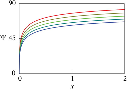
Figure 7. Computed net utility for different values of $\sigma$. In this figure, values of $\sigma$ are specified as 0.88 (red), 1.75 (brown), 2.63 (light green), 3.51 (deep green), and 4.38 (blue).

Figure 8. Computed net utility for different values of $r$. In this figure, values of $r$ are specified as 2.4 (red), 4.8 (brown), 7.2 (light green), 9.6 (deep green), and 12.0 (blue).

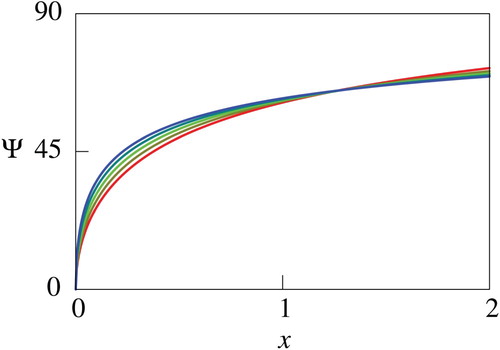
Figure 9. Computed net utility for different values of $a$. In this figure, values of $a$ are specified as $7.6\times {10}^{-3}$ (red), $7.6\times {10}^{-2}$ (brown), $7.6\times {10}^{-1}$ (light green), $7.6\times {10}^0$ (deep green), and $7.6\times {10}^1$ (blue).

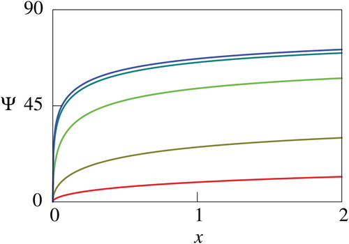
Figure 10. Computed net utility for different values of $b$. In this figure, values of $a$ are specified as $7.6\times {10}^{-3}$ (red), $7.6\times {10}^{-2}$ (brown), $7.6\times {10}^{-1}$ (light green), $7.6\times {10}^0$ (deep green), and $7.6\times {10}^1$ (blue).

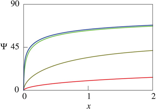
A comment on a consistency between the theoretical and numerical results are finally provided. The propositions in Section 3 are on theoretical results for the simplified model with $g=r$, while the numerical results are for the general model where $g$ is not a constant. Nevertheless, there are some consistency between the theoretical and numerical results. In fact, the parameter dependence of $\mathrm{\Psi }$ presented in Figures 6 through 10 agrees with the theoretical result of Proposition 3.3 except for large $x$ where $g<0$. This agreement would be because of the fact that the present $g$ approaches the constant $r$ when the body weight is small, namely when $x$ is small.

The computational results assess the impacts on the environmental and ecological model parameters on the fishery resource management from both qualitative and quantitative viewpoints. From a standpoint of robust fishery resources management, the obtained results theoretically support the empirics that the practitioners know. This paper can therefore be a first such attempt from a theoretical side.

5. Conclusions

A new stochastic differential game for management of non-renewable fishery resources subject to model ambiguity was formulated, and behaviour of the solutions to the HJBI equation and the associated optimal controls was analysed theoretically and numerically. The theoretical analysis with the exact solution implied the following things; to obtain higher net utility requires that the environment where the fishery resource is introduced is appropriately managed and the decision-maker has satisfactory knowledge about their population dynamics, so that the model ambiguity becomes small enough. The numerical analysis was also performed under a more realistic condition. The present mathematical modelling is a new attempt for effective management of non-renewable fishery resources. The exact and numerical solutions would be helpful for establishment of their management strategy. From the standpoint of robust fishery resources management, the mathematical and numerical analysis results in this paper supported the results that the practitioners have found.

Future research will focus on a problem where a part of a fishery resource is introduced into inland waters while the others are aquacultured. This kind of mixed management strategy is currently employed for P. altivelis in many inland fisheries cooperatives in Japan. The population dynamics model and the performance index will be then extended, so that the population dynamics of the released and aquacultured fishery resources [33,72] are concurrently managed. Human activities that were not focused on in this paper, such as taking countermeasures to suppress predation, can be handled with the present model. Another important topic to be addressed in future is coupling the present population dynamics model with a socio-economic model [4,44], so that fragility of the economy and society that rely on the fishery resources can be analysed. Modelling fishery resources management subject to catastrophic regime shifts [15,79] is also an interesting future research topic. For P. altivelis, sudden decrease of river water temperature triggers the fatal cold-water disease [28]. The presented model would serve as a key stone for approaching these advanced problems.

Acknowledgements

The authors thank Hii River Fishery Cooperatives for providing valuable comments on this research. The authors thank the reviewers for their helpful comments and suggestions.

Disclosure statement

No potential conflict of interest was reported by the authors.

ORCID

Hidekazu Yoshioka http://orcid.org/0000-0002-5293-3246

Additional information

Funding

This work was supported by Japan Society for the Promotion of Science [Grant Number 17J09125,17K15345]; Water Resources Environment Center [Grant Number 2016-02].

Appendices

Appendix A: Proofs of Propositions 2.1, 2.2, and 2.3.

This appendix provides proofs of Propositions 2.1, 2.2, and 2.3.

Proof of Proposition 2.1

The statement for $x$ is firstly proven. Given a triplet of controls $\left(c,\eta ,\omega \right)$ and $x_2\ge x_1\ge 0$, the two solutions $X_s^{\left(2\right)},X_s^{\left(1\right)}$ ($t\le s\le T$) to the SDE(2) subject to the initial conditions $x_2,x_1$ at $s=t-0$ satisfy $X_s^{\left(2\right)}\ge X_s^{\left(1\right)}\ge 0$ almost surely for $s\ge t$. This comparison result follows from a slight modification of Theorem 3 in Castro-Santis et al. [9] since both their and our problems are of the stochastic logistic type. The triplet of the optimizers $\left(c^{\ast },{\eta }^{\ast },{\omega }^{\ast }\right)$ for $\phi \left(t,n,x_i;c,\eta ,\omega \right)$ is denoted as $\left(c^{i\ast },{\eta }^{i\ast },{\omega }^{i\ast }\right)$ $(i=1,2)$. Then, $\phi \left(t,n,x_2;c,\eta ,\omega \right)\ge \phi \left(t,n,x_1;c,\eta ,\omega \right)$ by the form of $\phi$ in (3). We have (A1) $\phi \left(t,n,x_1;c,{\eta }^{2\ast },{\omega }^{2\ast }\right)\ge \phi \left(t,n,x_1;c,{\eta }^{1\ast },{\omega }^{1\ast }\right)$(A1) and (A2) $\phi \left(t,n,x_2;c,{\eta }^{2\ast },{\omega }^{2\ast }\right)\ge \phi \left(t,n,x_1;c,{\eta }^{2\ast },{\omega }^{2\ast }\right).$(A2) Combining (A1) and (A2) yields (A3) $\phi \left(t,n,x_2;c,{\eta }^{2\ast },{\omega }^{2\ast }\right)\ge \phi \left(t,n,x_1;c,{\eta }^{2\ast },{\omega }^{2\ast }\right)\ge \phi \left(t,n,x_1;c,{\eta }^{1\ast },{\omega }^{1\ast }\right),$(A3) and thus (A4) $\phi \left(t,n,x_2;c^{2\ast },{\eta }^{2\ast },{\omega }^{2\ast }\right)\ge \phi \left(t,n,x_2;c^{1\ast },{\eta }^{2\ast },{\omega }^{2\ast }\right)\ge \phi \left(t,n,x_1;c^{1\ast },{\eta }^{1\ast },{\omega }^{1\ast }\right).$(A4) This shows $\mathrm{\Phi }\left(t,n,x_2\right)\ge \mathrm{\Phi }\left(t,n,x_1\right)$ and the statement of the proposition for $x$ therefore follows. The statement for $n$ follows in the same way by observing that the two solutions $N_s^{\left(2\right)},N_s^{\left(1\right)}$ ($t\le s\le T$) to the SDE(1) subject to the initial conditions $n_2,n_1\ge 0$ at $s=t-0$ satisfy $N_s^{\left(2\right)}\ge N_s^{\left(1\right)}\ge 0$ almost surely for $s\ge t$.

Proof of Proposition 2.2

The statement for $r$ is firstly proven. Given a triplet of controls $\left(c,\eta ,\omega \right)$ and $r_2\ge r_1>0$, the two solutions $X_s^{\left(2\right)},X_s^{\left(1\right)}$ ($t\le s\le T$) to the SDE(2) subject to the initial conditions $X_{t-0}^{\left(1\right)}=X_{t-0}^{\left(2\right)}=x$ at $s=t-0$ satisfy $X_s^{\left(2\right)}\ge X_s^{\left(1\right)}\ge 0$ almost surely for $s\ge t$ as in the proof of Proposition 2.1. $\phi$ with $r=r_i$ is denoted as ${\phi }_i$ ($i=1,2$). The optimizer $\left(c^{\ast },{\eta }^{\ast },{\omega }^{\ast }\right)$ of ${\phi }_i$ is denoted as $\left(c^{i\ast },{\eta }^{i\ast },{\omega }^{i\ast }\right)$ $(i=1,2)$. Then, ${\phi }_2\ge {\phi }_1$ by (3). Straightforward calculation essentially the same with that of the proof of Proposition 2.1 proves the statement for $r$. The statement for $K$ follows in the same way.

Proof of Proposition 2.3

Given a triplet of controls $\left(c,\eta ,\omega \right)$, the integrand in (3) is increasing with respect to $w$, $a$, and $b$. The statement follows with a proof essentially the same with those of the Propositions 2.1 and 2.2.

Appendix B: Proofs of Propositions 3.1, 3.3, and 3.4.

This appendix provides proofs of Propositions 3.1, 3.3, and 3.4 stated in Section 3. Firstly, the proof of Proposition 3.1 is presented.

Proof of Proposition 3.1

For $z>0$, (19) can be expressed as (A5) $z=F\left(z\right)=\frac{1}{A}\left(\alpha z^{-1/\alpha }+B\right)$(A5) when $z\ge c_{max}^{-\alpha }$ and (A6) $G\left(z\right)=A{z}^2+\left[\left(1-\alpha \right)c_{max}-B\right]z-c_{max}^{1-\alpha }=0$(A6) when $0<z<c_{max}^{-\alpha }$. We have $z-F\left(z\right)\to -\mathrm{\infty }$ for $z\to +0$ and $z-F\left(z\right)\to +\mathrm{\infty }$ for $z\to +\mathrm{\infty }$, and $z-F\left(z\right)$ is strictly increasing with respect to $z>0$. Therefore, the classical intermediate value theorem shows that the equation (A5) has a unique positive solution $z=z_1>0$. By the above-mentioned geometric property of $z-F\left(z\right)$, the solution $z_1$ satisfies the condition $z_1\ge c_{max}^{-\alpha }$ when $c_{max}^{-\alpha }-F\left(c_{max}^{-\alpha }\right)\ge 0$, namely when (A7) $A\ge c_{max}^{\alpha }\left(\alpha c_{max}+B\right).$(A7) Next, on (A6), its positive solution $z=z_2$ exists uniquely and is expressed as (A8) $z_2=\frac{-u+\sqrt{u^2+4A{c}_{max}^{1-\alpha }}}{2A}$(A8) with (A9) $u=\left(1-\alpha \right)c_{max}-B.$(A9) The solution $z_2$ satisfies the condition $0<z_2<c_{max}^{-\alpha }$ when (A10) $0<\frac{-u+\sqrt{u^2+4A{c}_{max}^{1-\alpha }}}{2A}<c_{max}^{-\alpha }.$(A10) This condition is rewritten as (A11) $A<c_{max}^{\alpha }\left(\alpha c_{max}+B\right),$(A11) which is the complement of (A7). Therefore, we have shown that the solution to the equation (19) exists and is unique for both $z\ge c_{max}^{-\alpha }$ and $0<z<c_{max}^{-\alpha }$. This completes the proof.

Remark B.1

The unique solution $z=\hat{z}$ to the equation (19) is $z_1$ when (A7) and $z_2$ when (A11).

Secondly, the proof of Proposition 3.3 is presented.

Proof of Proposition 3.3

The proof is separated into the two cases, which are Case A: $z\ge c_{max}^{-\alpha }$ and Case B: $0<z<c_{max}^{-\alpha }$. For Case A, partially differentiating both-hand sides of (A5) for $z=\hat{z}$ with respect to $A$ yields (A12) $\begin{array}{rl}\frac{\mathrm{\partial }\hat{z}}{\mathrm{\partial }A}& =-\frac{1}{A^2}\left(\alpha {\hat{z}}^{-1/\alpha }+B\right)-\frac{1}{A}{\hat{z}}^{-\left(1+1/\alpha \right)}\frac{\mathrm{\partial }\hat{z}}{\mathrm{\partial }A}\\ & =-\frac{1}{A}\hat{z}-\frac{1}{A}{\hat{z}}^{-\left(1+1/\alpha \right)}\frac{\mathrm{\partial }\hat{z}}{\mathrm{\partial }A},\end{array}$(A12) which can be rewritten as (A13) $\frac{\mathrm{\partial }\hat{z}}{\mathrm{\partial }A}=-\frac{\hat{z}}{A+{\hat{z}}^{-\left(1+1/\alpha \right)}}<0.$(A13) Similarly, partially differentiating both-hand sides of (A5) for $z=\hat{z}$ with respect to $B$ yields (A14) $\frac{\mathrm{\partial }z}{\mathrm{\partial }B}=\frac{1}{A+z^{-\left(1+1/\alpha \right)}}>0.$(A14) The inequalities (A13) and (A14) prove the proposition for Case A. Indeed, (20) shows (A15) $\frac{\mathrm{\partial }A}{\mathrm{\partial }a}=-\frac{{\left(1-\alpha \right)}^2}{2a^2}<0$(A15) and thus (A16) $\frac{\mathrm{\partial }\hat{z}}{\mathrm{\partial }a}=\frac{\mathrm{\partial }\hat{z}}{\mathrm{\partial }A}\frac{\mathrm{\partial }A}{\mathrm{\partial }a}>0.$(A16) The statements on the other inequalities for Case A follow in the same way.

For Case B, the formula (A8) directly proves the proposition since (A17) $z_2=\frac{-u+\sqrt{u^2+4A{c}_{max}^{1-\alpha }}}{2A}=\frac{2c_{max}^{1-\alpha }}{u+\sqrt{u^2+4A{c}_{max}^{1-\alpha }}}$(A17) whose right-hand side is strictly decreasing with respect to $A$ and $u$. This observation with (20) and (A9) prove the proposition for Case B.

Finally, the proof of Proposition 3.4 is presented.

Proof of Proposition 3.4

The statements for the optimal controls are obvious due to their dependence on $\hat{z}$, except for the dependence of ${\eta }^{\ast }$ on $a$ and that of ${\omega }^{\ast }$ on $b$. Namely, we prove $\frac{\mathrm{\partial }{\eta }^{\ast }}{\mathrm{\partial }a}>0$ and $\frac{\mathrm{\partial }{\omega }^{\ast }}{\mathrm{\partial }b}>0$. Here, only the proof of the former is provided since the proof of the latter follows in the same way. The proof is separated in to the two cases, Case A: $z\ge c_{max}^{-\alpha }$ and Case B: $0<z<c_{max}^{-\alpha }$, as in the proof of Proposition 3.3. For both cases, we have (A18) $\frac{\mathrm{\partial }{\eta }^{\ast }}{\mathrm{\partial }a}=\frac{1-\alpha }{a}\hat{z}\left(\frac{1}{\hat{z}}\frac{\mathrm{\partial }\hat{z}}{\mathrm{\partial }A}-\frac{1}{a}\right),$(A18) and we show that the quantity $\frac{1}{\hat{z}}\frac{\mathrm{\partial }\hat{z}}{\mathrm{\partial }A}-\frac{1}{a}$ is negative.

For Case A, a direct computation with (A17) leads to (A19) $\begin{array}{rl}\frac{1}{\hat{z}}\frac{\mathrm{\partial }\hat{z}}{\mathrm{\partial }a}& =-\frac{1}{\hat{z}}\frac{{\hat{z}}^2}{\sqrt{u^2+4A{c}_{max}^{1-\alpha }}}\\ & =\frac{{\left(1-\alpha \right)}^2}{2a^2}\frac{\hat{z}}{\sqrt{u^2+4A{c}_{max}^{1-\alpha }}}\\ & <\frac{A\hat{z}}{a\sqrt{u^2+4A{c}_{max}^{1-\alpha }}}.\end{array}$(A19) Notice the relationship that is derived from (A8): (A20) $2A\hat{z}+u=\sqrt{u^2+4A{c}_{max}^{1-\alpha }}>0.$(A20) Combining (A19) and (A20) yields (A21) $\begin{array}{rl}a\left(\frac{1}{\hat{z}}\frac{\mathrm{\partial }\hat{z}}{\mathrm{\partial }a}-\frac{1}{a}\right)& <\frac{A\hat{z}}{2A\hat{z}+u}\\ & =\frac{A\hat{z}}{2A\hat{z}+u}-1\\ & =\frac{-\left(A\hat{z}+u\right)}{2A\hat{z}+u}.\end{array}$(A21) If $u\ge 0$, then (A21) shows (A22) $a\left(\frac{1}{\hat{z}}\frac{\mathrm{\partial }\hat{z}}{\mathrm{\partial }a}-\frac{1}{a}\right)<0,$(A22) which is the inequality to be proven. If $u<0$, by $0<z<c_{max}^{-\alpha }$, the right-hand side of (A21) is evaluated as (A23) $\frac{-\left(A\hat{z}+u\right)}{2A\hat{z}+u}<\frac{-\left(A{c}_{max}^{-\alpha }+u\right)}{2A{c}_{max}^{-\alpha }+u}$(A23) since $\frac{-\left(Az+u\right)}{2Az+u}$ is increasing with respect to $z$ when $2Az+u>0$. The condition (A11) then leads to (A24) $-\left(A{c}_{max}^{-\alpha }+u\right)<-u-\frac{\alpha }{1-\alpha }u-B=-\frac{\left(1-\alpha \right)c_{max}+\alpha }{1-\alpha }<0,$(A24) which again shows the desired inequality (A22).

For Case B, (A13) leads to (A25) $\begin{array}{rl}\frac{1}{\hat{z}}\frac{\mathrm{\partial }\hat{z}}{\mathrm{\partial }a}-\frac{1}{a}& =-\frac{1}{\hat{z}}\frac{\mathrm{\partial }A}{\mathrm{\partial }a}\frac{\hat{z}}{A+{\hat{z}}^{-\left(1+1/\alpha \right)}}-\frac{1}{a}\\ & =\frac{1}{a}\left(\frac{{\left(1-\alpha \right)}^2}{2a}\frac{1}{A+{\hat{z}}^{-\left(1+1/\alpha \right)}}-1\right)\\ & <\frac{1}{a}\left(\frac{A}{A+{\hat{z}}^{-\left(1+1/\alpha \right)}}-1\right)\\ & =\frac{-{\hat{z}}^{-\left(1+1/\alpha \right)}}{a\left(A+{\hat{z}}^{-\left(1+1/\alpha \right)}\right)}\\ & <0,\end{array}$(A25) which is the desired inequality. The proof is thus completed.

Appendix C: Discounted problem

This appendix gives theoretical results on a discounted problem, which seeks to optimize the performance index (A26) $\phi \left(t,n,x;c,\eta ,\omega \right)={\text{E}}^{n,x}\left[{\int }_t^T\frac{{\left(N_s{X}_s\right)}^{1-\alpha }}{1-\alpha }\left(J_1+J_2+J_3\right)\text{exp}\left(-\delta \left(s-t\right)\right)\text{d}s\right]$(A26) where $\delta >0$ is a discount factor, meaning that the fishery resource is managed from longer viewpoint with larger $\delta$. With the discounted performance index (A26), the HJBI equation and its reduced counterpart are derived as (A27) $-\frac{\mathrm{\partial \Phi }}{\mathrm{\partial }t}+\delta \mathrm{\Phi }+\underset{c\in \left[0,c_{max}\right]}{min}\underset{\eta ,\omega \in \mathbb{R}}{max}{L}_{c,\eta ,\omega }\mathrm{\Phi }=0$(A27) and (A28) $-\frac{\mathrm{\partial \Psi }}{\mathrm{\partial }t}+\delta \mathrm{\Psi }+\underset{c\in \left[0,c_{max}\right]}{min}\underset{\eta ,\omega \in \mathbb{R}}{max}{\hat{L}}_{c,\eta ,\omega }\mathrm{\Psi }=0,$(A28) respectively. The equations (A27) and (A28) have the corresponding linear decay terms. The reduced counterpart (A28) has mathematically the same structures with the non-discounted ones with an appropriate replacement of the parameters such as $\left(1-\alpha \right)R\to \left(1-\alpha \right)R+\delta$.

A quantity $\rho$ with the discount $\delta >0$ is denoted as ${\rho }_{\delta }$. The quantity without the discount is expressed as ${\rho }_0$. The definition (A26) of the discounted performance index and the above theoretical observation show the following results hold. Proposition C.1 is on the value function for the generalized logistic type $g$ and Proposition C.2 is on the exactly solvable case discussed in Section 3.

Proposition C.1

${\mathrm{\Phi }}_{\delta }$ is decreasing with respect to $\delta$.

Proposition C.2

$\frac{\mathrm{\partial }\mu }{\mathrm{\partial }\delta }<0$ where $\mu$ represents ${\hat{z}}_{\delta }$, $-{\eta }_{\delta }^{\ast }$, or $-{\omega }_{\delta }^{\ast }$. In addition, $\frac{\mathrm{\partial }{c}_{\delta }^{\ast }}{\mathrm{\partial }\delta }\le 0$.

All the propositions in the main text also hold for the discounted problem.

References

- M. Abdel-Hameed, Lévy Processes and Their Applications in Reliability and Storage, Springer, New York, 2014.
- S.I. Abe, Y. Tamaki, and K.I. Iguchi, Valuation of ecosystem services in restocking with ayu (Plecoglossus altivelis) in Japan. Proceedings of the Thirty-eighth US-Japan Aquaculture Panel Symposium, NOAA Technical Memorandum NMFS-F/SPO-113, Washington 2011; 47–51, 2011.
- E. Agliardi, Sustainability in uncertain economies, Environ. Resour. Econ. 48 (2011), pp. 71–82. doi:10.1007/s10640-010-9398-x.
- J. M. Anderies, Understanding the dynamics of sustainable social-ecological systems: human behavior, institutions, and regulatory feedback networks, Bull. Math. Biol. 77 (2015), pp. 259–280. doi:10.1007/s11538-014-0030-z.
- K. J. Arrow, Alternative approaches to the theory of choice in risk-taking situations, Econometrica. 19 (1951), pp. 404–437. doi:10.2307/1907465.
- B. K. Bhattacharjya, U. Bhaumik, and A. P. Sharma, Fish habitat and fisheries of Brahmaputra River in Assam, India, Aquat. Ecosyst. Health Manage. 20 (2017), pp. 102–115. doi: 10.1080/14634988.2017.1297171
- E. A. Blanchard, R. Loxton, and V. Rehbock, A computational algorithm for a class of non-smooth optimal control problems arising in aquaculture operations, Appl. Math. Comput. 219 (2013), pp. 8738–8746. doi:10.1016/j.amc.2013.02.070.
- D. A. Carlson, A. B. Haurie, A. Leizarowitz, Infinite Horizon Optimal Control: Deterministic and Stochastic Systems, Springer Science & Business Media, Berlin, 2012.
- R. Castro-Santis, F. Córdova-Lepe, and W. Chambio, An impulsive fishery model with environmental stochasticity. Feasibility, Math. Biosci. 277 (2016), pp. 71–76. doi:10.1016/j.mbs.2016.04.001.
- X. Chen, Y. Chen, T. Shimizu, J. Niu, K. I. Nakagami, X. Qian, … & J. Li, Water resources management in the urban agglomeration of the Lake Biwa region, Japan: An ecosystem services-based sustainability assessment, Sci. Total Environ. 586 (2017), pp. 174–187. doi:10.1016/j.scitotenv.2017.01.197.
- C.W. Clark, Bioeconomic Modelling and Fisheries Management, Wiley, New York, 1985.
- S. J. Cooke, E. H. Allison, T. D. Beard, R. Arlinghaus, A. H. Arthington, D. M. Bartley, … & A. J. Lynch, On the sustainability of inland fisheries: finding a future for the forgotten, Ambio. 45 (2016), pp. 753–764. doi:10.1007/s13280-016-0787-4.
- I. G. Cowx, Characterisation of inland fisheries in Europe, Fish. Manag. Ecol. 22 (2015), pp. 78–87. doi:10.1111/fme.12105.
- Ł. Delong and C. Klüppelberg, Optimal investment and consumption in a Black–Scholes market with Lévy-driven stochastic coefficients, Ann. Appl. Probab. 18 (2008), pp. 879–908. doi: 10.1214/07-AAP475
- A. De Zeeuw and X. He, Managing a renewable resource facing the risk of a regime shift in the ecological system, Resour. Energy Econ. 48 (2017), pp. 42–54. doi:10.1016/j.reseneeco.2017.01.003.
- E. Dockner, et al. Differential Games in Economics and Management Science, Cambridge University Press, Cambridge, 2000.
- L. Doyen and J. C. Péreau, Sustainable coalitions in the commons, Math. Soc. Sci. 63 (2012), pp. 57–64. doi:10.1016/j.mathsocsci.2011.10.006.
- G. W. Evatt, P. V. Johnson, P. W. Duck, and S. D. Howell, Optimal costless extraction rate changes from a non-renewable resource, Eur. J. Appl. Math. 25 (2014), pp. 681–705. doi:10.1017/S0956792514000229.
- E. P. Fenichel and J. K. Abbott, Heterogeneity and the fragility of the first best: putting the “micro” in bioeconomic models of recreational resources, Resour. Energy Econ. 36 (2014), pp. 351–369. doi:10.1016/j.reseneeco.2014.01.002.
- W. H. Fleming and H. M. Soner, Controlled Markov Processes and Viscosity Solutions (Vol. 25), Springer Science & Business Media, 2006.
- A. Gu, F. G. Viens, and B. Yi, Optimal reinsurance and investment strategies for insurers with mispricing and model ambiguity, Insurance Math. Econ. 72 (2017), pp. 235–249. doi:10.1016/j.insmatheco.2016.11.007.
- R. P. Gupta, M. Banerjee, and P. Chandra, The dynamics of two-species allelopathic competition with optimal harvesting, J. Biol. Dyn. 6 (2012), pp. 674–694. doi:10.1080/17513758.2012.677484.
- L. P. Hansen and T. J. Sargent, Misspecification in Recursive Macroeconomic Theory, Book Manuscript, New York University, New York, 2014.
- L. P. Hansen, T. J. Sargent, G. Turmuhambetova, and N. Williams, Robust control and model misspecification, J. Econ. Theory. 128 (2006), pp. 45–90. doi:10.1016/j.jet.2004.12.006.
- F. B. Hanson and D. Ryan, Optimal harvesting with both population and price dynamics, Math. Biosci. 148 (1998), pp. 129–146. doi:10.1016/S0025-5564(97)10011-6.
- N. Hritonenko, Y. Yatsenko, R. U. Goetz, and A. Xabadia, Optimal harvesting in forestry: steady-state analysis and climate change impact, J. Biol. Dyn. 7 (2013), pp. 41–58. doi:10.1080/17513758.2012.733425.
- K. I. Iguchi, K. Ogawa, M. Nagae, and F. Ito, The influence of rearing density on stress response and disease susceptibility of ayu (Plecoglossus altivelis), Aquaculture. 220 (2003), pp. 515–523. doi:10.1016/S0044-8486(02)00626-9.
- Y. Iida and A. Mizokami, Outbreaks of coldwater disease in wild ayu and pale chub, Fish. Pathol. 31 (1996), pp. 157–164. doi:10.3147/jsfp.31.157.
- H. Iwata, H. Takeshima, Y. Tago, K. Watanabe, K. Iguchi, and M. Nishida, Post-stocking dynamics of landlocked ayu Plecoglossus altivelis traced by a mitochondrial SNP marker, Nippon Suisan Gakkaishi. 73 (2007), pp. 278–283. doi:10.2331/suisan.73.278.
- B. G. Jang and S. Park, Ambiguity and optimal portfolio choice with value-at-risk constraint, Finance Res. Lett. 18 (2016), pp. 158–176. doi:10.1016/j.frl.2016.04.013.
- A. B. Johannesen and A. Skonhoft, Growth and measurement uncertainty in an unregulated fishery, Nat. Resour. Model. 22 (2009), pp. 370–392. doi:10.1111/j.1939-7445.2009.00041.x.
- D. Karimanzira, K. Keesman, W. Kloas, D. Baganz, and T. Rauschenbach, Efficient and economical way of operating a recirculation aquaculture system in an aquaponics farm, Aquacult. Econ. Manage. (2016), pp. 1–18. doi:10.1080/13657305.2016.1259368.
- O. Katano, H. Hakoyama, S. Shinichiro, Japanese inland fisheries and aquaculture: status and trends. in Freshwater Fisheries Ecology, J. E. Craig, eds., John Wiley and Sons, Ltd, UK, 2012, pp. 231–240. doi:10.1002/9781118394380.ch20.
- K. Kugarajh, L. K. Sandal, and G. Berge, Implementing a stochastic bioeconomic model for the North-East Arctic cod fishery, J. Bioecon. 8 (2006), pp. 35–53. doi:10.1007/s10818-005-5783-x.
- G. Lafforgue, Stochastic technical change, non-renewable resource and optimal sustainable growth, Resour Energy Econ. 30 (2008), pp. 540–554. doi:10.1016/j.reseneeco.2008.07.001.
- S. D. Langhans, J. Gessner, V. Hermoso, and C. Wolter, Coupling systematic planning and expert judgement enhances the efficiency of river restoration, Sci. Total Environ. 560 (2016), pp. 266–273. doi:10.1016/j.scitotenv.2016.03.232.
- T. Le and C. Le Van, Transitional dynamics in an R&D-based growth model with natural resources, Math. Soc. Sci. 82 (2016), pp. 1–17. doi:10.1016/j.mathsocsci.2016.04.001.
- M. Longo and A. Mainini, Learning and portfolio decisions for CRRA investors, Int. J. Theor. Appl. Finance, 19 (2016), pp. 1650018. doi:10.1142/S0219024916500187.
- K. Lorenzen, I. G. Cowx, R. E. M. Entsua-Mensah, N. P. Lester, J. D. Koehn, R. G. Randall, and S. D. Bower, Stock assessment in inland fisheries: a foundation for sustainable use and conservation, Rev. Fish. Biol. Fish. 26 (2016), pp. 405–440. doi:10.1007/s11160-016-9435-0.
- A. J. Lynch, S. J. Cooke, A. M. Deines, S. D. Bower, D. B. Bunnell, I. G. Cowx, and M. W. Rogers, The social, economic, and environmental importance of inland fish and fisheries, Environ. Rev. 24 (2016), pp. 115–121. doi:10.1139/er-2015-0064.
- P. J. Maenhout, Robust portfolio rules and detection-error probabilities for a mean-reverting risk premium, J. Econ. Theory. 128 (2006), pp. 136–163. doi:10.1016/j.jet.2005.12.012.
- J. Marín-Solano and J. Navas, Consumption and portfolio rules for time-inconsistent investors, Eur. J. Oper. Res. 201 (2010), pp. 860–872. doi:10.1016/j.ejor.2009.0W4.005. doi: 10.1016/j.ejor.2009.04.005
- J. Marín-Solano and E. V. Shevkoplyas, Non-constant discounting and differential games with random time horizon, Automatica (Oxf). 47 (2011), pp. 2626–2638. doi:10.1016/j.automatica.2011.09.010.
- S. Marsiglio and D. La Torre, Economic growth and abatement activities in a stochastic environment: a multi-objective approach, Ann. Oper. Res. (2016), pp. 1–14. doi:10.1007/s10479-016-2357-3.
- T. Marutani, On the optimal path in the dynamic pool model for a fishery, Rev. Fish. Biol. Fish. 18 (2008), pp. 133–141. doi:10.1007/s11160-007-9065-7.
- S. Mataramvura and B. Øksendal, Risk minimizing portfolios and HJBI equations for stochastic differential games, Stochastics Int. J. Probab. Stochastic Processes. 80 (2008), pp. 317–337. doi:10.1080/17442500701655408.
- R. Matsuyama, N. Kuninaga, T. Morimoto, T. Shibano, A. Sudo, K. Sudo, and T. Asai, Isolation and antimicrobial susceptibility of Plesiomonas shigelloides from great cormorants (Phalacrocorax carbo hanedae) in Gifu and Shiga Prefectures, Japan, J. Vet. Med. Sci. 77 (2015), pp. 1179–1181. doi:10.1292/jvms.15-0014.
- S. I. S. Matsuzaki and T. Kadoya, Trends and stability of inland fishery resources in Japanese lakes: introduction of exotic piscivores as a driver, Ecol. Appl. 25 (2015), pp. 1420–1432. doi:10.1890/13-2182.1.
- G. Moscarini and L. Smith, The optimal level of experimentation, Econometrica. 69 (2011), pp. 1629–1644. doi:10.1111/1468-0262.00259.
- J. Miao and A. Rivera, Robust contracts in continuous time, Econometrica. 84 (2016), pp. 1405–1440. doi:10.3982/ECTA13127.
- K. Muraoka, K. Amano, T. Doi, H. Kubota, and J. Miwa Effects of suspended solid concentrations and particle size on survival of Ayu (Plecoglossus altivelis altivelis), Jpn. J. Ichthyol. 58 (2011), pp. 141–151. ( in Japanese with English Abstract) doi:10.11369/jji.58.141.
- J. D. Murray, Mathematical Biology, Springer, Berlin, 1993.
- A. S. Nowak, A multigenerational dynamic game of resource extraction, Math. Soc. Sci. 51 (2006), pp. 327–336. doi:10.1016/j.mathsocsci.2005.12.003.
- B. Øksendal, & A. Sulem, Applied Stochastic Control of Jump Diffusions, Springer-Verlag Berlin Heidelberg, 2007.
- J. W. Pratt, Risk aversion in the small and in the large, Econometrica. 32 (1964), pp. 122–136. doi:10.1007/978-94-015-7957-5_3. doi: 10.2307/1913738
- N. Privault, Notes on Stochastic Finance. Available at http://www.ntu.edu.sg/home/nprivault/indext.html.
- M. Rechencq, P. H. Vigliano, G. E. Lippolt, M. F. Alonso, P. J. Macchi, P. A. Alvear, and M. V. Fernandez, Modelling and management options for salmonid sport fisheries: A case study from Patagonia, Argentina, Fish. Manag. Ecol. 24 (2017), pp. 103–116. doi:10.1111/fme.12208.
- F. J. Richards, A flexible growth function for empirical use, J. Exp. Bot. 10 (1959), pp. 290–300. doi:10.1093/jxb/10.2.290.
- J. V. Ross, A note on density dependence in population models, Ecol. Modell. 220 (2009), pp. 3472–3474. doi:10.1016/j.ecolmodel.2009.08.024.
- W. Steffens, Great Cormorant–substantial danger to fish populations and fishery in Europe, Bulg. J. Agric. Sci. 16 (2010), pp. 322–331.
- Y. Tago, Survival of a landlocked form of Ayu fry released in the Shou River, Aquacult. Sci. 47 (1999), pp. 111–112. (in Japanese with English Abstract) doi:10.11233/aquaculturesci1953.47.111.
- K. Takamura, Invasive species from the highly endemic fish fauna of Lake Biwa threatening freshwater fish in rivers of the Kanto region, Jpn. J. Limnol. (Rikusuigaku Zasshi). 70 (2009), pp. 249–253. (in Japanese with English Abstract) doi:10.3739/rikusui.70.249.
- G. Vardas, A. Xepapadeas, Uncertainty aversion, robust control and asset holdings, Quant. Finance, 15 (2015), pp. 477–491. doi:10.1080/14697688.2011.637077.
- H. Wang, Robust asset pricing with stochastic hyperbolic discounting, Finance Res. Lett. 21 (2017), pp. 178–185. doi:10.1016/j.frl.2017.01.005.
- A. Xepapadeas and C. Roseta-Palma, Instabilities and robust control in natural resource management, Portuguese Econ. J. 12 (2013), pp. 161–180. doi:org/10.1007/s10258-013-0092-0.
- H. Xiang, C. C. Zhu, and H. F. Huo, Modelling the effect of immigration on drinking behaviour, J. Biol. Dyn. 11 (2017), pp. 275–298. doi:10.1080/17513758.2017.1337243.
- Y. Yaegashi, H. Yoshioka, K. Unami, and M. Fujihara, Numerical simulation of a Hamilton-Jacobi-Bellman equation for optimal management strategy of released Plecoglossus altivelis in river systems, Model Design Simul. Anal. Commun. Comput. Inf. Sci. 603 (2016) (Chi S.D. and Ohn S.Y., Eds.), Springer Science+Business Media Singapore, pp. 91–101. doi:10.1007/978-981-10-2158-9_8.
- Y. Yaegashi, H. Yoshioka, K. Unami, and M. Fujihara, An optimal management strategy for stochastic population dynamics of released Plecoglossus altivelis in rivers, Int. J. Model. Simul. Sci. Comput. 8 (2017), pp. 1750039, 16pp. doi:10.1142/S1793962317500398.
- Y. Yaegashi, H. Yoshioka, K. Unami, and M. Fujihara, Optimal policy of predator suppression for sustainable inland fishery management, Proceedings of 12th SDEWES Conference, Dubrovnik, Croatia, Proceedings, pp. 309-1–309-11, 2017.
- B. Yi, Z. Li, F. G. Viens, and Y. Zeng, Robust optimal control for an insurer with reinsurance and investment under Heston’s stochastic volatility model, Insurance Math. Econ. 53 (2013), pp. 601–614. doi:10.1016/j.insmatheco.2013.08.011.
- H. Yoshioka, K. Unami, M. Fujihara, Mathematical analysis on a conforming finite element scheme for advection-dispersion-decay equations on connected graphs, J. Jpn. Soc. Civil Eng. A2, 70 (2014), pp. I_265–I_274. doi:10.2208/jscejam.70.I_265.
- H. Yoshioka and Y. Yaegashi, Finding the optimal opening time of harvesting farmed fishery resources, Pac. J. Math. Ind. 8 (2016), pp. 6. doi:10.1186/s40736-016-0025-9.
- H. Yoshioka and Y. Yaegashi Optimization model to start harvesting in stochastic aquaculture system, Appl. Stoch. Models Bus. Ind. 33 (2017), pp. 476–493. doi:10.1002/asmb.2250.
- H. Yoshioka and Y. Yaegashi, Optimization model of aquacultured fish for selling and ecological education, J. Math. Ind. 7 (2017). doi: 10.1186/s13362-017-0038-8
- H. Yoshioka, & Y. Yaegashi Mathematical analysis for management of released fish, Optimal Control Appl. Methods. doi:10.1002/oca.2392/full (Accepted on Nov. 13, 2017)
- H. Yoshioka, & Y. Yaegashi Stochastic control model of dam discharge for algae growth management, J. Biol. Dyn. 12 (2018), pp. 242–270. doi: 10.1080/17513758.2018.1436197
- H. Yoshioka and Y. Yaegashi, Robust stochastic control modeling of dam discharge to suppress overgrowth of downstream harmful algae, Appl. Stoch. Models Bus. Ind. (in press). doi:10.1002/asmb.2301.
- R. Yu and P. Leung, Optimal partial harvesting schedule for aquaculture operations, Mar. Resour. Econ. 21 (2006), pp. 301–315. doi:10.1086/mre.21.3.42629513.
- A. Zemel, Precaution under mixed uncertainty: implications for environmental management, Resour. Energy Econ. 34 (2012), pp. 188–197. doi:10.1016/j.reseneeco.2011.11.002.
- Y. Zeng, D. Li, and A. Gu, Robust equilibrium reinsurance-investment strategy for a mean–variance insurer in a model with jumps, Insurance: Math. Econ. 66 (2016), pp. 138–152. doi:10.1016/j.insmatheco.2015.10.012.
- Z. Zhang, X. Zhang, and J. Tong, Exponential ergodicity for population dynamics driven by α-stable processes, Stat. Probab. Lett. 125 (2017), pp. 149–159. doi:10.1016/j.spl.2017.02.010.
- X. Zou and K. Wang, Optimal harvesting for a logistic population dynamics driven by a Lévy process, J. Optim. Theory Appl. 161 (2014), pp. 969–979. doi:10.1007/s10957-013-0451-0.