Complex contagion leads to complex dynamics in models coupling behaviour and disease

ABSTRACT

Models coupling behaviour and disease as two unique but interacting contagions have existed since the mid 2000s. In these coupled contagion models, behaviour is typically treated as a ‘simple contagion’. However, the means of behaviour spread may in fact be more complex. We develop a family of disease-behaviour coupled contagion compartmental models in order to examine the effect of behavioural contagion type on disease-behaviour dynamics. Coupled contagion models treating behaviour as a simple contagion and a complex contagion are investigated, showing that behavioural contagion type can have a significant impact on dynamics. We find that a simple contagion behaviour leads to simple dynamics, while a complex contagion behaviour supports complex dynamics with the possibility of bistability and periodic orbits.

KEYWORDS:

• Mathematical epidemiology
• behaviour
• coupled contagion
• compartmental model
• bistability
• periodic orbits

1. Introduction

The desire to better understand the interaction between disease and behaviour has led to the development of ‘coupled contagion models’ (see e.g. [15–17, 21, 40, 44, 51, 54–57]) in which both disease and behaviour are treated as contagious processes and subsequently coupled. Typically these models treat both contagions as ‘simple contagions’, assuming recruitment can occur through a single contact. However, an added complication is that mechanisms for behavioural contagion may differ from those for disease transmission. For example, behavioural change might occur through ‘complex contagions’, where adoption requires reinforcement or contact from multiple sources [6, 8, 38, 48]. The objective of this paper is to study the dynamic implications of simple versus complex behavioural contagion in the coupling of behaviour and disease. We shall show that when behaviour is viewed as a complex contagion, complex disease dynamics can arise in a family of ordinary differential equation (ODE) models that couple behaviour and disease.

Recognition of infectious disease as a contagious process dates back to the establishment of the germ theory of disease [47], and the use of mathematical models for describing disease dynamics has a long history [2, 3, 30]. In contrast, mathematical modelling of the spread of ideas and behavioural change as a contagion is of more recent origin, with frameworks such as ‘susceptible-infectious-susceptible’ (SIS) dynamics being adopted for modelling ‘thought contagion’ [20, 36]. The coupling of disease and behaviour has long been recognized, and continues to be critically important to public health. Proper condom usage [5, 29] and treatment seeking [33] are behaviours that directly impact the incidence and prevalence of sexually transmitted infections (STIs). On the other hand, disease may also impact behaviour. For example, the outbreak of HIV in the 1980s led to an ‘epidemic’ of stigma against HIV-positive individuals [26, 37].

There has been recent interest in developing and understanding mathematical models that combine behaviour and disease dynamics as coupled contagions [11, 15, 16, 21, 33, 40, 44, 51, 54–57]. This interest stems both from applied and theoretical interest. Fu, Christakis, and Fowler [13] recently presented empirical evidence that the absence of behaviour as a contagion from models can lead to faulty predictions of critical disease statistics such as the basic reproduction number and final outbreak size [13]. Indeed, understanding how and to what extent behaviour should be explicitly incorporated into infectious disease models is one of the largest challenges facing mathematical modellers of infectious disease [14]. On the other hand, understanding coupled contagion dynamics is of theoretical interest as well, as this coupling can result in dynamics that do not occur when the two are uncoupled [1].

In much of the existing coupled contagion literature, behavioural contagion is modelled as a ‘simple contagion’ [11, 15, 16, 21, 33, 40, 44, 51, 55–57]. With a simple contagion the spread of the contagion requires only a single contact, often being modelled with mass action incidence. However, it is possible that some behaviours require multiple exposures and/or social reinforcement to spread [6, 8, 38, 48]. Contagions that spread in this manner will be referred to as ‘complex contagions’. The effect that behavioural contagion type has on coupled disease-behaviour dynamics is not well understood. The intention of this paper is to help fill this gap.

In this paper, we present an ODE coupled contagion framework that allows us to compare the qualitative differences between a coupled contagion model treating behaviour as a simple contagion and one that treats behaviour as a complex contagion. We show that the complex contagion model provides much richer dynamics, having the potential for unforced oscillations and bistability in certain parameter regimes.

The remainder of the paper is organized as follows. Section 2 presents the general model in which disease and behaviour are coupled, followed by the stability analysis of the disease-free equilibrium (DFE) based on the derived basic reproduction number. Sections 3 and 4 insert behaviour into our general model as a simple and complex contagion, respectively. Particularly, a thorough bifurcation analysis is conducted for the simple behavioural contagion model in Section 3; a detailed equilibrium analysis is carried out in a special case for a complex behavioural contagion model and more general investigations are addressed with numerical results in Section 4. Final conclusions and remarks are given in Section 5.

2. The general model

We present a model coupling disease with a behaviour that inhibits disease spread.

The basic structure builds upon SIS dynamics for both disease and behaviour, with coupling of the two contagion processes via the respective incidence terms. Let S denote the proportion of the population that is susceptible to disease, I the proportion that is infected, U the proportion that has not adopted (i.e. are ‘susceptible’ to) the behaviour, and A the proportion that has adopted (i.e. are ‘infected’ with) the behaviour.

The general family of models we consider is: (1) $\begin{array}{rl}\dot{S}& =-\beta h\left(A\right)SI+\gamma I,\\ \dot{I}& =\beta h\left(A\right)SI-\gamma I,\\ \dot{U}& =-\alpha \ell \left(I\right)g(U,A)+\xi A,\\ \dot{A}& =\alpha \ell \left(I\right)g(U,A)-\xi A.\end{array}$(1) Incorporated into system (1(1) $\begin{array}{rl}\dot{S}& =-\beta h\left(A\right)SI+\gamma I,\\ \dot{I}& =\beta h\left(A\right)SI-\gamma I,\\ \dot{U}& =-\alpha \ell \left(I\right)g(U,A)+\xi A,\\ \dot{A}& =\alpha \ell \left(I\right)g(U,A)-\xi A.\end{array}$(1) ) are the following assumptions:

1. There is no explicit tracking of behaviour status within the disease compartments, or of disease status within the behaviour compartments (i.e. the S, I, U, and A compartments are not divided into sub-compartments).

2. Both disease transmission and behaviour adoption are assumed to occur through the interaction between ‘susceptible’ and ‘infected’ individuals with respect to the corresponding contagion.

3. behaviour prevalence modulates disease transmission, for example by altering the probability that a contact leads to disease transmission.

4. Disease prevalence modulates behaviour transmission, again by altering the probability that a contact results in behaviour transmission.

Assumptions (iii) and (iv) are the basis of how disease and behaviour are coupled in the family of models we consider. In particular, the $h\left(A\right)$ and $\ell \left(I\right)$ terms in system (1(1) $\begin{array}{rl}\dot{S}& =-\beta h\left(A\right)SI+\gamma I,\\ \dot{I}& =\beta h\left(A\right)SI-\gamma I,\\ \dot{U}& =-\alpha \ell \left(I\right)g(U,A)+\xi A,\\ \dot{A}& =\alpha \ell \left(I\right)g(U,A)-\xi A.\end{array}$(1) ) correspond to how behaviour prevalence modulates disease incidence and how disease prevalence modulates behaviour incidence, respectively. We will assume throughout that $h\left(A\right)$ and $\ell \left(I\right)$ are continuous on $[0,1]$, continuously differentiable on $(0,1)$, and satisfy:

1. $h\left(0\right)=1$.

2. $0\le h\left(A\right)\le 1$ for $A\in [0,1]$.

3. $h^{\prime }\left(A\right)\le 0$ for $A\in (0,1)$.

4. $\ell \left(0\right)=0$.

5. $0\le \ell \left(I\right)\le 1$ for $I\in [0,1]$.

6. ${\ell }^{\prime }\left(I\right)\ge 0$ for $I\in (0,1)$.

We are thus considering protective behaviours that limit disease transmission, assume that motivation to adopt behaviour increases with the perception of disease risk, and assume that in the absence of disease the system will converge to a population where no one adopts the behaviour.

Assumption (i) is an approximation, and will not hold in situations where disease and behaviour status are highly dependent. An advantage of assumption (i) is that it reduces the dimension of the system, allowing for analytic results and biological insight into how different behavioural contagion processes affect disease dynamics that could otherwise be obfuscated by more complicated approaches. There are furthermore situations where this approximation may be reasonable. As a motivating example, consider condom usage and gonorrhoea among men who have sex with men. SIS models have been used to model gonorrhoea, including the classical work of Hethcote and Yorke (1984) [27]. A high proportion of gonorrhoea infections are asymptomatic, and thus condom usage being independent of an individual's infection status may be a reasonable approximation (assumption (i)). Perceived costs of condom usage can be significant [39], leading to unprotected sex in some cases, and condom usage would likely decline if neither disease nor birth control was concerns. Condom use decreases the transmission of sexually transmitted infections (STIs), and it is possible that condom usage would increase with increased prevalence and perceived risk of STIs such as gonorrhoea [19] (assumption (iii)). Sexual behaviours are intimate and changes in sexual behaviour may be heavily influenced by direct interaction with individuals exhibiting the behaviour or advocating behaviour change [31, 43, 46] (assumption (ii)). We note that condom usage is variable within an individual between sex acts [12, 41], and thus behaviour adoption may correspond to changes in the frequency of condom usage (e.g. ‘unadopted’ corresponding to rarely uses a condom, and ‘adopted’ corresponding to often uses a condom) rather than an all or nothing outcome.

Throughout the paper, we fix the disease transmission process to follow mass action kinetics and investigate the effects of varying the form of the behavioural contagion incidence term. Contacts between U and A individuals are modelled with $g(U,A)$. The actual form of g depends upon the behavioural contagion type being considered, as we will discuss in the following sections.

Taking S+I=U+A=1 (conservation of the population) allows for the following reduced model: (2) $\begin{array}{rl}\dot{I}& =\beta h\left(A\right)(1-I)I-\gamma I,\\ \dot{A}& =\alpha \ell \left(I\right)f\left(A\right)-\xi A,\end{array}$(2) where $f\left(A\right)=g\left(\right(1-A),A)$.

Figure 1 below is a flow diagram of the model and Table 1 is an accompanying parameter table. We will use the requirements for the parameters listed in Table 1 in various proofs throughout the paper without explicitly stating them. Also for the remainder of this paper let Ω denote $[0,1]\times [0,1]$ where I is the first coordinate and A is the second coordinate. This is the biologically relevant region for model (2(2) $\begin{array}{rl}\dot{I}& =\beta h\left(A\right)(1-I)I-\gamma I,\\ \dot{A}& =\alpha \ell \left(I\right)f\left(A\right)-\xi A,\end{array}$(2) ).

Figure 1. Compartmental transition diagram for model (1(1) $\begin{array}{rl}\dot{S}& =-\beta h\left(A\right)SI+\gamma I,\\ \dot{I}& =\beta h\left(A\right)SI-\gamma I,\\ \dot{U}& =-\alpha \ell \left(I\right)g(U,A)+\xi A,\\ \dot{A}& =\alpha \ell \left(I\right)g(U,A)-\xi A.\end{array}$(1) ). Red indicates disease contributions, and blue indicates behavioural contributions. Note the coupling of both processes is the mutual modulation of rates, $\beta h\left(A\right)$ for disease and $\alpha \ell \left(I\right)$ for behaviour.

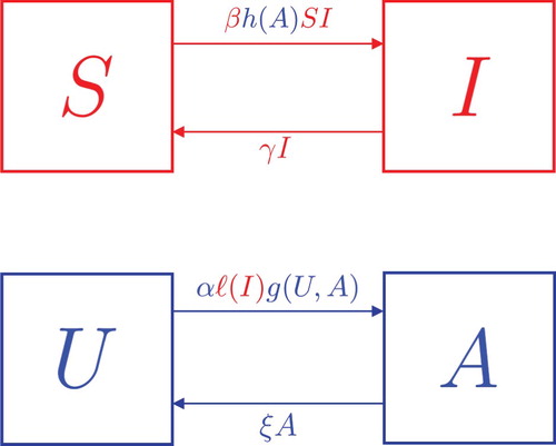
Table 1. Reference table for model (4(4) $\begin{array}{rl}\dot{I}& =\beta h\left(A\right)(1-I)I-\gamma I,\\ \dot{A}& =\alpha If\left(A\right)-\xi A.\end{array}$(4) ) that provides a definition of relevant parameters and regions.

Symbol	Meaning	Requirements
β	Disease transmission rate	$>0$
γ	Recovery rate	$>0$
α	Behavioural adoption rate	$>0$
ξ	Forgetting rate	$>0$
Ω	Biologically relevant region	$[0,1]\times [0,1]$

In the following sections, we will make two choices for $g(U,A)$, one that corresponds to simple contagion and another corresponding to complex contagion. First, however, there are some features of this framework that will hold regardless of the choice of $g(U,A)$. The first such result is the form of the disease's basic reproduction number, ${\mathcal{R}}_0$. Assuming that $h\left(A\right)$ is differentiable at A=0 and $\ell \left(I\right)$ is differentiable at I=0, we use the next generation matrix approach [9, 53] with $(I,A)=(0,0)$ as the DFE. The basic reproduction number for (2(2) $\begin{array}{rl}\dot{I}& =\beta h\left(A\right)(1-I)I-\gamma I,\\ \dot{A}& =\alpha \ell \left(I\right)f\left(A\right)-\xi A,\end{array}$(2) ) is found to be: (3) ${\mathcal{R}}_0=\frac{\beta }{\gamma }.$(3) Note that (3(3) ${\mathcal{R}}_0=\frac{\beta }{\gamma }.$(3) ) does not depend upon behaviour. This is because behaviour adoption is contingent upon disease prevalence, which is 0 at the DFE. The absence of behaviour related parameters in (3(3) ${\mathcal{R}}_0=\frac{\beta }{\gamma }.$(3) ) paired with the following result will show that in model (2(2) $\begin{array}{rl}\dot{I}& =\beta h\left(A\right)(1-I)I-\gamma I,\\ \dot{A}& =\alpha \ell \left(I\right)f\left(A\right)-\xi A,\end{array}$(2) ) despite the presence of a preventative behaviour disease still becomes endemic when ${\mathcal{R}}_0>1$, meaning that behaviour does not alter the disease invasion threshold.

Theorem 2.1

The DFE of system (2(2) $\begin{array}{rl}\dot{I}& =\beta h\left(A\right)(1-I)I-\gamma I,\\ \dot{A}& =\alpha \ell \left(I\right)f\left(A\right)-\xi A,\end{array}$(2) ) is globally asymptotically stable in Ω when ${\mathcal{R}}_0\le 1$ and unstable when ${\mathcal{R}}_0>1$.

Proof.

Suppose ${\mathcal{R}}_0\le 1$. Following the Lyapunov function used by Eisenberg et al. (2013) [10] let $V\left(I\right)={\mathcal{R}}_{0}I$. V is positive definite on Ω and $\dot{V}=\beta {\mathcal{R}}_{0}I(1-I)h\left(A\right)-\beta I$. It holds that $\dot{V}<0$ on $\mathrm{\Omega }\setminus \{I=0\}$. If I=0 then $\dot{V}=0$ and if $\dot{V}=0$ it holds that $I\le 0$. Thus on Ω we have that $\dot{V}=0$ if and only if I=0. Therefore the system decays to $\{I=0\}.$ By assumption (2), restricting the system to $\{I=0\}$ shows that all trajectories approach the DFE as $t\to \mathrm{\infty }$. Thus the DFE of system (2(2) $\begin{array}{rl}\dot{I}& =\beta h\left(A\right)(1-I)I-\gamma I,\\ \dot{A}& =\alpha \ell \left(I\right)f\left(A\right)-\xi A,\end{array}$(2) ) must be globally asymptotically stable when ${\mathcal{R}}_0\le 1$.

If ${\mathcal{R}}_0>1$ then Theorem 2 of van den Driessche and Watmough (2002) gives that the DFE is unstable [53].

The finding that behaviour change alone is insufficient to prevent disease outbreaks is a common feature of models where disease is required for behaviour adoption [15, 16, 33]. However as we will see in the following two sections, behavioural contagion can have an impact on the future course of a disease once an outbreak has occurred.

For the remainder of the paper we take $\ell \left(I\right)=I$. This choice gives a simple functional form relating perceived disease risk to disease prevalence and is convenient for mathematical analysis. We expect similar qualitative dynamics for $\ell \left(I\right)$ monotone increasing and concave down on $(0,1)$.

This final assumption gives our reduced model the following form: (4) $\begin{array}{rl}\dot{I}& =\beta h\left(A\right)(1-I)I-\gamma I,\\ \dot{A}& =\alpha If\left(A\right)-\xi A.\end{array}$(4)

3. Behaviour as a simple contagion

For behaviours that spread as a simple contagion, we take $g(U,A)=UA$. This corresponds to behaviour transmission following mass action kinetics, resulting in the reduced system: (5) $\begin{array}{rl}\dot{I}& =\beta h\left(A\right)(1-I)I-\gamma I\\ \dot{A}& =\alpha I(1-A)A-\xi A.\end{array}$(5) This approach follows from the social science literature [20, 36], and many prior coupled contagion models utilize mass action kinetics as well [11, 15, 16, 33, 40, 51].

The simplicity of (5(5) $\begin{array}{rl}\dot{I}& =\beta h\left(A\right)(1-I)I-\gamma I\\ \dot{A}& =\alpha I(1-A)A-\xi A.\end{array}$(5) ) allows for a full analysis without reliance on numerical tools. We show below that our model is able to recover similar dynamics to other coupled contagion models that treat behaviour as a simple contagion. In particular, the dynamics of our behavioural simple contagion model mimic those of models in which disease compartments are broken into sub-compartments that denote behavioural status [11, 15, 16, 33, 40, 51].

3.1. Analysis and results

The right hand side of (5(5) $\begin{array}{rl}\dot{I}& =\beta h\left(A\right)(1-I)I-\gamma I\\ \dot{A}& =\alpha I(1-A)A-\xi A.\end{array}$(5) ) is continuously differentiable everywhere $h\left(A\right)$ is continuously differentiable, and thus for initial conditions starting in the interior of Ω there exist unique solutions. Checking the system on the boundary guarantees that any trajectory that starts in Ω remains in Ω for all time; that is, the domain Ω is positively invariant for model (5(5) $\begin{array}{rl}\dot{I}& =\beta h\left(A\right)(1-I)I-\gamma I\\ \dot{A}& =\alpha I(1-A)A-\xi A.\end{array}$(5) ).

We are now interested in finding all steady states in which disease is present. In order to do this we first introduce a key parameter for determining when behaviour is able to invade the system: (6) ${\mathcal{R}}_b=\frac{\alpha }{\xi }.$(6) Note that ${\mathcal{R}}_b$ can be interpreted as a reproduction number for information in system (5(5) $\begin{array}{rl}\dot{I}& =\beta h\left(A\right)(1-I)I-\gamma I\\ \dot{A}& =\alpha I(1-A)A-\xi A.\end{array}$(5) ). Specifically, in a completely unadopted population the number of secondary adopters that a single adopter produces during its lifespan is ${\mathcal{R}}_b$.

There are possibly two distinct fixed points with nonzero disease prevalence. The first can be found by setting $\dot{I}$ and $\dot{A}$ equal to 0. When ${\mathcal{R}}_0>1$ this gives a biologically meaningful endemic point, $(1-1/{\mathcal{R}}_0,0)$. To prove the existence of the other point we look at the intersection of the interior nullclines of system (5(5) $\begin{array}{rl}\dot{I}& =\beta h\left(A\right)(1-I)I-\gamma I\\ \dot{A}& =\alpha I(1-A)A-\xi A.\end{array}$(5) ).

Theorem 3.1

The A-nullcline, $I_A\left(A\right)=1/{\mathcal{R}}_b(1-A)$, and the I-nullcline, $I_I\left(A\right)=1-1/{\mathcal{R}}_{0}h\left(A\right)$, of system (5(5) $\begin{array}{rl}\dot{I}& =\beta h\left(A\right)(1-I)I-\gamma I\\ \dot{A}& =\alpha I(1-A)A-\xi A.\end{array}$(5) ) intersect exactly once in the interior of Ω when $0<1/{\mathcal{R}}_b<1-1/{\mathcal{R}}_0$ and never in the interior of Ω when $1/{\mathcal{R}}_b\ge 1-1/{\mathcal{R}}_0\ge 0$ .

Proof.

$I_A^{\prime }\left(A\right)>0$ and $I_I^{\prime }\left(A\right)\le 0$ on $[0,1)$. Thus the absolute minimum for $I_A$ on $[0,1)$ is $I_A\left(0\right)=1/{\mathcal{R}}_b$. The absolute maximum for $I_I$ on $[0,1)$ is $I_I\left(0\right)=1-1/{\mathcal{R}}_0$.

Suppose $0<1/{\mathcal{R}}_b<1-1/{\mathcal{R}}_0$. Then because $\underset{A\to 1}{lim}{I}_A\left(A\right)=\mathrm{\infty }$, and $I_A$ is continuous and strictly increasing on $[0,1)$ it must hold that $I_A$ and $I_I$ cross exactly once inside the interior of Ω.

On the other hand if $1/{\mathcal{R}}_b\ge 1-1/{\mathcal{R}}_0\ge 0$ it is not possible for $I_A$ and $I_I$ to intersect inside the interior of Ω.

The equilibrium that results from Theorem 3.1 will be denoted as $(I^{\ast },A^{\ast })$ and will be referred to as the coexistence point of system (5(5) $\begin{array}{rl}\dot{I}& =\beta h\left(A\right)(1-I)I-\gamma I\\ \dot{A}& =\alpha I(1-A)A-\xi A.\end{array}$(5) ). This is because it is a steady state where both disease and behaviour prevalence are nonzero. It can be seen from the proof of Theorem 3.1 that $I^{\ast }<1-1/{\mathcal{R}}_0$, therefore when behaviour is present there is a lower disease prevalence.

We now see that model (5(5) $\begin{array}{rl}\dot{I}& =\beta h\left(A\right)(1-I)I-\gamma I\\ \dot{A}& =\alpha I(1-A)A-\xi A.\end{array}$(5) ) has at most three biologically relevant fixed points, (7) $(I,A)=(0,0),$(7) (8) $(I,A)=(1-\frac{1}{{\mathcal{R}}_0},0)\mathrm{when}{\mathcal{R}}_0>1,$(8) (9) $(I,A)=(I^{\ast },A^{\ast })\mathrm{when}{\mathcal{R}}_0\ge \frac{{\mathcal{R}}_b}{{\mathcal{R}}_b-1}\ge 0.$(9) From the previous section we have a full understanding of how the DFE is affected by the infectiousness of both the disease and behaviour contagions. We would like to know under which conditions, if any, the endemic and coexistence points are stable.

As a first step towards this stability analysis, we show that for any choice of parameters system (5(5) $\begin{array}{rl}\dot{I}& =\beta h\left(A\right)(1-I)I-\gamma I\\ \dot{A}& =\alpha I(1-A)A-\xi A.\end{array}$(5) ) does not allow for periodic solutions.

Theorem 3.2

System (5(5) $\begin{array}{rl}\dot{I}& =\beta h\left(A\right)(1-I)I-\gamma I\\ \dot{A}& =\alpha I(1-A)A-\xi A.\end{array}$(5) ) does not admit periodic orbits in Ω.

Proof.

Let $B(I,A)=1/IA$. Then in $\mathrm{\Omega \setminus }\{A=0\}$ $\frac{\mathrm{\partial }\left(B\dot{I}\right)}{\mathrm{\partial }I}=\frac{-\beta h\left(A\right)}{A}\le 0,\text{ and }\frac{\mathrm{\partial }\left(B\dot{A}\right)}{\mathrm{\partial }A}=-\alpha <0.\text{ Thus }\frac{\mathrm{\partial }\left(B\dot{I}\right)}{\mathrm{\partial }I}+\frac{\mathrm{\partial }\left(B\dot{A}\right)}{\mathrm{\partial }A}<0,$ and so by the Bendixson–Dulac criterion there is no periodic orbit in $\mathrm{\Omega \setminus }\{A=0\}$.

On the set $\{A=0\}$ our system becomes: $\begin{array}{rl}\dot{I}& =\beta (1-I)I-\gamma I\\ \dot{A}& =0\end{array},$ which will tend to $(0,0)$ or $(1-1/{\mathcal{R}}_0,0)$ as $t\to \mathrm{\infty }$.

Thus for any choice of parameters system (5(5) $\begin{array}{rl}\dot{I}& =\beta h\left(A\right)(1-I)I-\gamma I\\ \dot{A}& =\alpha I(1-A)A-\xi A.\end{array}$(5) ) does not admit periodic solutions.

Theorems 3.3 and 3.4 below show that when ${\mathcal{R}}_0$ is greater than one but below ${\mathcal{R}}_b/({\mathcal{R}}_b-1)$, then almost all solution trajectories approach the endemic equilibrium, whereas for ${\mathcal{R}}_0>{\mathcal{R}}_b/({\mathcal{R}}_b-1)$ the coexistence point is globally asymptotically stable.

Theorem 3.3

The endemic equilibrium of (5(5) $\begin{array}{rl}\dot{I}& =\beta h\left(A\right)(1-I)I-\gamma I\\ \dot{A}& =\alpha I(1-A)A-\xi A.\end{array}$(5) ) is globally asymptotically stable in $\mathrm{\Omega }\setminus \{I=0\}$ when $1<{\mathcal{R}}_0<{\mathcal{R}}_b/\left({\mathcal{R}}_b-1\right)$ and is unstable otherwise.

Proof.

The Jacobian of (5(5) $\begin{array}{rl}\dot{I}& =\beta h\left(A\right)(1-I)I-\gamma I\\ \dot{A}& =\alpha I(1-A)A-\xi A.\end{array}$(5) ) evaluated at (8(8) $(I,A)=(1-\frac{1}{{\mathcal{R}}_0},0)\mathrm{when}{\mathcal{R}}_0>1,$(8) ) is $\left(\begin{array}{cc}\gamma -\beta & \ast \\ 0& \alpha (1-\frac{1}{{\mathcal{R}}_0})-\xi \end{array}\right),$ where $\ast$ denotes some nonzero entry we do not need because our matrix is upper triangular. When ${\mathcal{R}}_0>1$ it holds that $\gamma -\beta <0$. The other eigenvalue is strictly negative when ${\mathcal{R}}_0<{\mathcal{R}}_b/\left({\mathcal{R}}_b-1\right)$. Thus the endemic point is locally asymptotically stable when $1<{\mathcal{R}}_0<{\mathcal{R}}_b/\left({\mathcal{R}}_b-1\right)$. In this regime the only two fixed points in the invariant set Ω are (7(7) $(I,A)=(0,0),$(7) ) and (8(8) $(I,A)=(1-\frac{1}{{\mathcal{R}}_0},0)\mathrm{when}{\mathcal{R}}_0>1,$(8) ). The unstable manifold of the DFE goes from the DFE along the I-axis into the endemic point, while the stable manifold of the DFE corresponds to the I=0 axis. This rules out a homoclinic orbit emanating out of the DFE. Note also that for $1<{\mathcal{R}}_0<{\mathcal{R}}_b/\left({\mathcal{R}}_b-1\right)$ the coexistence point (9(9) $(I,A)=(I^{\ast },A^{\ast })\mathrm{when}{\mathcal{R}}_0\ge \frac{{\mathcal{R}}_b}{{\mathcal{R}}_b-1}\ge 0.$(9) ) does not exist in the biologically relevant region. Together with Theorems 2.1 and 3.2, for $1<{\mathcal{R}}_0<{\mathcal{R}}_b/\left({\mathcal{R}}_b-1\right)$ we have that the endemic equilibrium (8(8) $(I,A)=(1-\frac{1}{{\mathcal{R}}_0},0)\mathrm{when}{\mathcal{R}}_0>1,$(8) ) is the only attractor for the planar system (5(5) $\begin{array}{rl}\dot{I}& =\beta h\left(A\right)(1-I)I-\gamma I\\ \dot{A}& =\alpha I(1-A)A-\xi A.\end{array}$(5) ), and thus is globally asymptotically stable on $\mathrm{\Omega }\setminus \{I=0\}$. Finally, when ${\mathcal{R}}_0$ is not in $(1,{\mathcal{R}}_b/({\mathcal{R}}_b-1\left)\right)$ the Jacobian has at least one strictly positive eigenvalue, so the endemic point is unstable.

Theorem 3.4

If ${\mathcal{R}}_0>{\mathcal{R}}_b/\left({\mathcal{R}}_b-1\right)>0$ point (9(9) $(I,A)=(I^{\ast },A^{\ast })\mathrm{when}{\mathcal{R}}_0\ge \frac{{\mathcal{R}}_b}{{\mathcal{R}}_b-1}\ge 0.$(9) ) of system (5(5) $\begin{array}{rl}\dot{I}& =\beta h\left(A\right)(1-I)I-\gamma I\\ \dot{A}& =\alpha I(1-A)A-\xi A.\end{array}$(5) ) is globally asymptotically stable on the set $\mathrm{\Omega }\setminus \left(\right\{A=0\}\cup \{I=0\left\}\right)$.

Proof.

Suppose ${\mathcal{R}}_0>{\mathcal{R}}_b/\left({\mathcal{R}}_b-1\right)>0$. By Theorems 2.1 and 3.3 both the DFE and endemic point are unstable, and from Theorem 3.2 there are no periodic solutions. Note also that the DFE and endemic point have one dimensional stable manifolds corresponding to the I=0 and A=0 axes, respectively, and thus saddle connections involving these fixed points do not exist. As system (5(5) $\begin{array}{rl}\dot{I}& =\beta h\left(A\right)(1-I)I-\gamma I\\ \dot{A}& =\alpha I(1-A)A-\xi A.\end{array}$(5) ) is planar, we conclude that solution trajectories starting in the interior of Ω must approach the coexistence point as $t\to \mathrm{\infty }$. Therefore (9(9) $(I,A)=(I^{\ast },A^{\ast })\mathrm{when}{\mathcal{R}}_0\ge \frac{{\mathcal{R}}_b}{{\mathcal{R}}_b-1}\ge 0.$(9) ) is globally asymptotically stable.

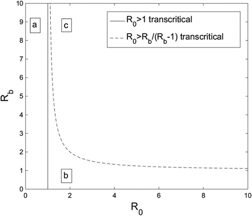
Theorems 3.3 and 3.4 imply that the dynamics of system (5(5) $\begin{array}{rl}\dot{I}& =\beta h\left(A\right)(1-I)I-\gamma I\\ \dot{A}& =\alpha I(1-A)A-\xi A.\end{array}$(5) ) are completely determined by ${\mathcal{R}}_0$ and ${\mathcal{R}}_b$. The ${\mathcal{R}}_0$-${\mathcal{R}}_b$ parameter plane is presented below in Figure 2 with bifurcation curves that break the plane into three distinct dynamical regions. The ${\mathcal{R}}_0=1$ curve corresponds to a transcritical bifurcation where disease (but not behaviour) invades the system, and is a common feature in disease models. In addition, there exists a second curve of transcritical bifurcations at ${\mathcal{R}}_0={\mathcal{R}}_b/\left({\mathcal{R}}_b-1\right)$, where points (8(8) $(I,A)=(1-\frac{1}{{\mathcal{R}}_0},0)\mathrm{when}{\mathcal{R}}_0>1,$(8) ) and (9(9) $(I,A)=(I^{\ast },A^{\ast })\mathrm{when}{\mathcal{R}}_0\ge \frac{{\mathcal{R}}_b}{{\mathcal{R}}_b-1}\ge 0.$(9) ) collide and exchange stability. Information invasion and behavioural change correspond to crossing this latter curve of transcriticals.

Figure 2. The ${\mathcal{R}}_0$-${\mathcal{R}}_b$ parameter space broken into three regions by the transcritical bifurcation curves for system (5(5) $\begin{array}{rl}\dot{I}& =\beta h\left(A\right)(1-I)I-\gamma I\\ \dot{A}& =\alpha I(1-A)A-\xi A.\end{array}$(5) ). In region (a) The DFE is the sole biologically relevant fixed point, and it is globally stable. In (b) (7(7) $(I,A)=(0,0),$(7) ) and (8(8) $(I,A)=(1-\frac{1}{{\mathcal{R}}_0},0)\mathrm{when}{\mathcal{R}}_0>1,$(8) ) exist in Ω, with (8(8) $(I,A)=(1-\frac{1}{{\mathcal{R}}_0},0)\mathrm{when}{\mathcal{R}}_0>1,$(8) ) globally stable. In region (c) all three fixed points are present in Ω, and point (9(9) $(I,A)=(I^{\ast },A^{\ast })\mathrm{when}{\mathcal{R}}_0\ge \frac{{\mathcal{R}}_b}{{\mathcal{R}}_b-1}\ge 0.$(9) ) is globally asymptotically stable. Figure generated in MATLAB.

There are three dynamical features of system (5(5) $\begin{array}{rl}\dot{I}& =\beta h\left(A\right)(1-I)I-\gamma I\\ \dot{A}& =\alpha I(1-A)A-\xi A.\end{array}$(5) ) that we wish to highlight. First, the disease invasion threshold is not altered by behaviour in model (5(5) $\begin{array}{rl}\dot{I}& =\beta h\left(A\right)(1-I)I-\gamma I\\ \dot{A}& =\alpha I(1-A)A-\xi A.\end{array}$(5) ). This is expected because our behavioural adoption function, $\alpha IA(1-A)$, is modulated by disease prevalence. Previous prevalence-driven compartmental coupled contagion models [15, 16, 33] have observed this same feature. Second, disease infection drives behaviour adoption, in that ${\mathcal{R}}_0$ must be sufficiently large in order for behaviour adoption to occur. Indeed, for any ${\mathcal{R}}_b>1$ there exists a region for ${\mathcal{R}}_0$, namely $(1,{\mathcal{R}}_b/({\mathcal{R}}_b-1\left)\right)$, where disease is present but not behaviour. Again this reflects the fact that behaviour transmission requires the presence of disease in system (5(5) $\begin{array}{rl}\dot{I}& =\beta h\left(A\right)(1-I)I-\gamma I\\ \dot{A}& =\alpha I(1-A)A-\xi A.\end{array}$(5) ). Other studies have found similar results, as Funk et. al. (2009) found that awareness spreads only when sufficiently many carry the disease [16], Wang et al. (2014) found that information propagation is promoted by disease spreading [56], and Granell et al. (2013) found that increasing disease infectivity can also increase the fraction of aware individuals [21]. Finally, we also find that when behaviour is able to invade, disease prevalence at the attracting fixed point is lowered. Again this is expected, as lowered prevalence should occur when a behaviour that prevents disease spread is considered [11, 15, 16, 21, 33, 40, 44, 51, 55–57]. System (5(5) $\begin{array}{rl}\dot{I}& =\beta h\left(A\right)(1-I)I-\gamma I\\ \dot{A}& =\alpha I(1-A)A-\xi A.\end{array}$(5) ) has been sufficiently analysed and we can now examine the differences that occur with a complex contagion approach for behaviour spread.

4. Behaviour as a complex contagion

To model behaviour as a complex contagion we take $g(U,A)=U{A}^2/\left({\delta }^2+A^2\right)$, where δ is the Hill activation coefficient. This gives the reduced system: (10) $\begin{array}{rl}\dot{I}& =\beta h\left(A\right)(1-I)I-\gamma I,\\ \dot{A}& =\frac{\alpha I(1-A)A^2}{{\delta }^2+A^2}-\xi A.\end{array}$(10) A Hill function is utilized to emulate the cooperativity required in spreading a complex contagion. Repeated exposures are necessary for the transmission of complex contagions. When prevalence is very low (e.g. a single individual), repeated exposures do not occur and thus there is very little or no transmission. Now consider the force of behavioural infection with the Hill function in system (10(10) $\begin{array}{rl}\dot{I}& =\beta h\left(A\right)(1-I)I-\gamma I,\\ \dot{A}& =\frac{\alpha I(1-A)A^2}{{\delta }^2+A^2}-\xi A.\end{array}$(10) ), $\alpha I{A}^2/\left({\delta }^2+A^2\right)$. Similar to the complex contagion scenario described above, the rate of change of the force of infection is 0 when A=0, with an accelerating force of infection for sufficiently low information prevalence. Specifically, the Hill function has positive curvature for $A<\delta /\sqrt{3}$. Note also that the force of infection begins to plateau as A increases, indicating a saturation effect that occurs when individuals that do not exhibit the behaviour are difficult to encounter. This saturation effect begins to occur as the curvature of the force of infection becomes negative when $A>\delta /\sqrt{3}$.

Hill functions have been widely used as a nonlinear force of infection term in the disease modelling literature [28, 34, 35]. In particular, it is a specific instance of a general class of function used to model diseases that require multiple exposures for spread and exhibit the saturation effect [34]. Empirical evidence for behavioural complex contagion, where multiple concurrent exposures are required for transmission, has been documented in several different settings [6, 38, 48].

We use a Hill function here as a mathematically simple incidence function that captures the initial acceleration of the force of infection with prevalence, a key feature of complex contagion. However, whether or not the analytical results of this choice for $g(U,A)$ generalize to a broader class of functions is beyond the scope of the presented work. We comment further on the potential for generalization in Section 5.

In the remainder of the paper we will assume that $\delta \in [0,\sqrt{3}]$, so that both cooperativity and saturation in the force of infection for behaviour can occur in the biologically relevant range $0\le A\le 1$.

4.1. Analysis and results

Next we examine the the dynamics of system (10(10) $\begin{array}{rl}\dot{I}& =\beta h\left(A\right)(1-I)I-\gamma I,\\ \dot{A}& =\frac{\alpha I(1-A)A^2}{{\delta }^2+A^2}-\xi A.\end{array}$(10) ). Model (10(10) $\begin{array}{rl}\dot{I}& =\beta h\left(A\right)(1-I)I-\gamma I,\\ \dot{A}& =\frac{\alpha I(1-A)A^2}{{\delta }^2+A^2}-\xi A.\end{array}$(10) ) is more complicated than (5(5) $\begin{array}{rl}\dot{I}& =\beta h\left(A\right)(1-I)I-\gamma I\\ \dot{A}& =\alpha I(1-A)A-\xi A.\end{array}$(5) ) and as such numerical tools will be relied upon. When the need for numerical tools arises the generality of $h\left(A\right)$ will be dropped in favour of a specific function.

The right hand side of (10(10) $\begin{array}{rl}\dot{I}& =\beta h\left(A\right)(1-I)I-\gamma I,\\ \dot{A}& =\frac{\alpha I(1-A)A^2}{{\delta }^2+A^2}-\xi A.\end{array}$(10) ) is continuously differentiable everywhere as $h\left(A\right)$ is continuously differentiable. The vector field points inward on the boundary of the compact set Ω, and thus there exist unique solutions in all of Ω, and any solution that begins in Ω remains in Ω for all positive time.

Our goal is to describe the dynamics of system (10(10) $\begin{array}{rl}\dot{I}& =\beta h\left(A\right)(1-I)I-\gamma I,\\ \dot{A}& =\frac{\alpha I(1-A)A^2}{{\delta }^2+A^2}-\xi A.\end{array}$(10) ). For this we will continue to use the notation ${\mathcal{R}}_b=\alpha /\xi$, however, it is important to note that in system (10(10) $\begin{array}{rl}\dot{I}& =\beta h\left(A\right)(1-I)I-\gamma I,\\ \dot{A}& =\frac{\alpha I(1-A)A^2}{{\delta }^2+A^2}-\xi A.\end{array}$(10) ) ${\mathcal{R}}_b$ loses its previous biological interpretation. Here ${\mathcal{R}}_b$ only gives an upper bound on the number of secondary adopters an adopter can create. Once we incorporate cooperativity an adopter's ability to spread the behaviour becomes more complicated, but ${\mathcal{R}}_b$ still plays an important role.

To understand the dynamics of model (10(10) $\begin{array}{rl}\dot{I}& =\beta h\left(A\right)(1-I)I-\gamma I,\\ \dot{A}& =\frac{\alpha I(1-A)A^2}{{\delta }^2+A^2}-\xi A.\end{array}$(10) ) we again look for non-DFE fixed points. Solving $\dot{I}=0$ and $\dot{A}=0$ simultaneously we find that $(1-1/{\mathcal{R}}_0,0)$ is also an equilibrium for this system. We will refer to this point as the endemic point of model (10(10) $\begin{array}{rl}\dot{I}& =\beta h\left(A\right)(1-I)I-\gamma I,\\ \dot{A}& =\frac{\alpha I(1-A)A^2}{{\delta }^2+A^2}-\xi A.\end{array}$(10) ).

While behaviour was able to destabilize the endemic point of model (5(5) $\begin{array}{rl}\dot{I}& =\beta h\left(A\right)(1-I)I-\gamma I\\ \dot{A}& =\alpha I(1-A)A-\xi A.\end{array}$(5) ), the same is not true of the endemic point of model (10(10) $\begin{array}{rl}\dot{I}& =\beta h\left(A\right)(1-I)I-\gamma I,\\ \dot{A}& =\frac{\alpha I(1-A)A^2}{{\delta }^2+A^2}-\xi A.\end{array}$(10) ).

Theorem 4.1

If ${\mathcal{R}}_0>1$ the endemic fixed point of system (10(10) $\begin{array}{rl}\dot{I}& =\beta h\left(A\right)(1-I)I-\gamma I,\\ \dot{A}& =\frac{\alpha I(1-A)A^2}{{\delta }^2+A^2}-\xi A.\end{array}$(10) ) is locally stable.

Proof.

The Jacobian of (10(10) $\begin{array}{rl}\dot{I}& =\beta h\left(A\right)(1-I)I-\gamma I,\\ \dot{A}& =\frac{\alpha I(1-A)A^2}{{\delta }^2+A^2}-\xi A.\end{array}$(10) ) evaluated at the endemic point is: $\left(\begin{array}{cc}\gamma -\beta & \ast \\ 0& -\xi \end{array}\right),$ where $\ast$ denotes a potentially nonzero entry. Both eigenvalues are strictly negative when ${\mathcal{R}}_0>1$. Thus the endemic point is locally asymptotically stable when ${\mathcal{R}}_0>1$.

Theorem 4.1 suggests that merely introducing a deterrent behaviour into the population is not enough to alter the course of an already established infectious disease in system (10(10) $\begin{array}{rl}\dot{I}& =\beta h\left(A\right)(1-I)I-\gamma I,\\ \dot{A}& =\frac{\alpha I(1-A)A^2}{{\delta }^2+A^2}-\xi A.\end{array}$(10) ). In order to better understand the role behaviour plays in system (10(10) $\begin{array}{rl}\dot{I}& =\beta h\left(A\right)(1-I)I-\gamma I,\\ \dot{A}& =\frac{\alpha I(1-A)A^2}{{\delta }^2+A^2}-\xi A.\end{array}$(10) ) we look for other nontrivial equilibria. Once again we look to the intersection of nullclines in the interior of Ω to prove their existence.

Lemma 4.2

A necessary condition for the existence of equilibria for system (10(10) $\begin{array}{rl}\dot{I}& =\beta h\left(A\right)(1-I)I-\gamma I,\\ \dot{A}& =\frac{\alpha I(1-A)A^2}{{\delta }^2+A^2}-\xi A.\end{array}$(10) ) in the interior of Ω is ${\mathcal{R}}_0>\left({\mathcal{R}}_b(-\delta +\sqrt{{\delta }^2+1})\right)/\left({\mathcal{R}}_b(-\delta +\sqrt{{\delta }^2+1})-2\delta \right)\ge 1$.

Proof.

Interior equilibria for system (10(10) $\begin{array}{rl}\dot{I}& =\beta h\left(A\right)(1-I)I-\gamma I,\\ \dot{A}& =\frac{\alpha I(1-A)A^2}{{\delta }^2+A^2}-\xi A.\end{array}$(10) ) correspond to intersections of the nullclines $I_A\left(A\right)=\left({\delta }^2+A^2\right)/{\mathcal{R}}_b(1-A)A$ and $I_I\left(A\right)=1-1/{\mathcal{R}}_{0}h\left(A\right)$ in $(0,1)$. $I_A^{\prime }=0$ only when $A=(-\delta \pm \sqrt{{\delta }^2+1})\delta$, and of these two critical points only $A^{\ast }=(-\delta +\sqrt{{\delta }^2+1})\delta$ is in $(0,1)$. As $I_A$ is continuously differentiable on $(0,1)$ and $\underset{A\to 0^{+}}{lim}{I}_A=\underset{A\to 1^{-}}{lim}{I}_A=\mathrm{\infty }$ it holds that $I_A$ has a global minimum at $A^{\ast }$. Thus the smallest value of $I_A$ in $(0,1)$ is $I_A\left(A^{\ast }\right)=2\delta /\left({\mathcal{R}}_b(-\delta +\sqrt{{\delta }^2+1})\right)$. From the proof of Theorem 3.1 we have that $I_I$ is monotone decreasing on $[0,1]$ and thus $\underset{A\in (0,1)}{sup}{I}_I\left(A\right)=I_I\left(0\right)=1-1/{\mathcal{R}}_0$.

Interior equilibria correspond to intersections of $I_A$ and $I_I$ in $(0,1)$. This is only possible when $sup{I}_I\ge min{I}_A$, which corresponds to ${\mathcal{R}}_0>\left({\mathcal{R}}_b(-\delta +\sqrt{{\delta }^2+1})\right)/\left({\mathcal{R}}_b\right(-\delta +\sqrt{{\delta }^2+1})-2\delta )\ge 1$.

Lemma 4.2 gives a condition for when interior equilibria are possible for system (10(10) $\begin{array}{rl}\dot{I}& =\beta h\left(A\right)(1-I)I-\gamma I,\\ \dot{A}& =\frac{\alpha I(1-A)A^2}{{\delta }^2+A^2}-\xi A.\end{array}$(10) ). Whether interior equilibria in fact occur when this condition is met depends upon the specific choice of $h\left(A\right)$.

To further study the dynamics of system (10(10) $\begin{array}{rl}\dot{I}& =\beta h\left(A\right)(1-I)I-\gamma I,\\ \dot{A}& =\frac{\alpha I(1-A)A^2}{{\delta }^2+A^2}-\xi A.\end{array}$(10) ), we set $h\left(A\right)=1-A$ for the remainder of the section. This choice gives a force of disease infection $\beta (1-A)I$ that can be interpreted as random, independent mixing with respect to disease and behaviour status, with behaviour adoption conferring complete protection from disease infection.

Under this choice of $h\left(A\right)$ we can give an exact parameter regime for the existence of other fixed points. As with model (5(5) $\begin{array}{rl}\dot{I}& =\beta h\left(A\right)(1-I)I-\gamma I\\ \dot{A}& =\alpha I(1-A)A-\xi A.\end{array}$(5) ) we use the term coexistence point when referring to a fixed point with both nonzero I and A.

Theorem 4.3

Let ${\mathcal{R}}_b>2/\left(-1+\sqrt{1+(1/\delta {)}^2}\right)$ for system (10(10) $\begin{array}{rl}\dot{I}& =\beta h\left(A\right)(1-I)I-\gamma I,\\ \dot{A}& =\frac{\alpha I(1-A)A^2}{{\delta }^2+A^2}-\xi A.\end{array}$(10) ) with $h\left(A\right)=1-A$. Then we have the following trichotomy:

1. For ${\mathcal{R}}_0<1/\left(1-2\delta \sqrt{1/{\mathcal{R}}_b+(1/{\mathcal{R}}_b{)}^2}\right)$ there are no coexistence points in $\stackrel{\circ }{\mathrm{\Omega }}$,

2. For ${\mathcal{R}}_0=1/\left(1-2\delta \sqrt{1/{\mathcal{R}}_b+(1/{\mathcal{R}}_b{)}^2}\right)$ there is a single coexistence point in $\stackrel{\circ }{\mathrm{\Omega }}$,

3. For ${\mathcal{R}}_0>1/\left(1-2\delta \sqrt{1/{\mathcal{R}}_b+(1/{\mathcal{R}}_b{)}^2}\right)$ there are two distinct coexistence points in $\stackrel{\circ }{\mathrm{\Omega }}$,

where $\stackrel{\circ }{\mathrm{\Omega }}$ is referred to as the interior of Ω.

Proof.

To find interior fixed points we set the nullclines from Lemma 4.2 equal to one another and solve for A. Solving $I_I\left(A\right)=I_A\left(A\right)$ for A gives: $A_{\pm }=\frac{(1-\frac{1}{{\mathcal{R}}_0})\pm \sqrt{{(1-\frac{1}{{\mathcal{R}}_0})}^2-4(1+\frac{1}{{\mathcal{R}}_b})\frac{{\delta }^2}{{\mathcal{R}}_b}}}{2}(1+\frac{1}{{\mathcal{R}}_b}).$ The square root term is real precisely when $(1-1/{\mathcal{R}}_0{)}^2-4{\delta }^2(1/{\mathcal{R}}_b+\left(1/{\mathcal{R}}_b{)}^2\right)\ge 0$, which happens when $1-1/{\mathcal{R}}_0\ge 2\delta \sqrt{1/{\mathcal{R}}_b+(1/{\mathcal{R}}_b{)}^2}$ or $1-1/{\mathcal{R}}_0\le -2\delta \sqrt{\begin{array}{c}1/{\mathcal{R}}_b+\\ (1/{\mathcal{R}}_b{)}^2\end{array}}$. However, we can ignore the latter inequality because Lemma 4.2 tells us that in order for interior equilibria to exist it must hold that ${\mathcal{R}}_0\ge 1$. Thus we are left with $1-1/{\mathcal{R}}_0\ge 2\delta \sqrt{1/{\mathcal{R}}_b+(1/{\mathcal{R}}_b{)}^2}$ or rather $1-2\delta \sqrt{1/{\mathcal{R}}_b+(1/{\mathcal{R}}_b{)}^2}\ge 1/{\mathcal{R}}_0$. In order for this inequality to hold it must be true that ${\mathcal{R}}_b>2/(-1+\sqrt{1+(1/\delta {)}^2})$ because ${\mathcal{R}}_0\ge 0$, i.e. the square root term can only be real if ${\mathcal{R}}_b>2/(-1+\sqrt{1+(1/\delta {)}^2})$ and ${\mathcal{R}}_0\ge 1/(1-2\delta \sqrt{1/{\mathcal{R}}_b+(1/{\mathcal{R}}_b{)}^2})$.

Let $r=1/(1-2\delta \sqrt{1/{\mathcal{R}}_b+(1/{\mathcal{R}}_b{)}^2})$. When ${\mathcal{R}}_0<r$ the square root term is negative, and so no intersection points occur in $\stackrel{\circ }{\mathrm{\Omega }}$. If ${\mathcal{R}}_0=r$ the square root term is 0 and thus the two nullclines have exactly one intersection point in $\stackrel{\circ }{\mathrm{\Omega }}$. Finally, if ${\mathcal{R}}_0>r$ the square root term is strictly positive and hence it follows from $0<A_{-}<A_{+}<1$ that there are two distinct intersection points in $\stackrel{\circ }{\mathrm{\Omega }}$.

The transition from zero to two coexistence points described in Theorem 4.3 as ${\mathcal{R}}_0$ crosses r corresponds to a saddle-node bifurcation, where r denotes the value presented in the proof of Theorem 4.3.

As in the simple contagion model (5(5) $\begin{array}{rl}\dot{I}& =\beta h\left(A\right)(1-I)I-\gamma I\\ \dot{A}& =\alpha I(1-A)A-\xi A.\end{array}$(5) ), disease needs to be sufficiently contagious for coexistence equilibria to exist in the complex contagion model (10(10) $\begin{array}{rl}\dot{I}& =\beta h\left(A\right)(1-I)I-\gamma I,\\ \dot{A}& =\frac{\alpha I(1-A)A^2}{{\delta }^2+A^2}-\xi A.\end{array}$(10) ) as well. However, the bifurcations underlying behaviour invasion for the two classes of models differ, with a transcritical bifurcation and loss of stability of the endemic point for simple behavioural contagions, versus a saddle-node bifurcation for complex behavioural contagions. This difference has practical implications for disease control. Consider a population that is at the endemic equilibrium, where disease is present but behaviour absent. Suppose that a preventative behaviour is introduced in an effort to lessen disease prevalence. Under simple behavioural contagion, introducing a small amount of behaviour change can lead to a sustained decrease in disease prevalence, whereas under complex behavioural contagion a lasting reduction in disease prevalence requires sufficiently large initial introduction of behaviour for the system to leave the basin of attraction of the endemic point.

Theorems 2.1, 4.1, and 4.3 also provide us with a parameter region in which the endemic point of system (10(10) $\begin{array}{rl}\dot{I}& =\beta h\left(A\right)(1-I)I-\gamma I,\\ \dot{A}& =\frac{\alpha I(1-A)A^2}{{\delta }^2+A^2}-\xi A.\end{array}$(10) ) is globally stable in $\mathrm{\Omega }\setminus \{I=0\}$.

Corollary 4.4

If either 4.4 or 4.4 below hold then the endemic point of system (10(10) $\begin{array}{rl}\dot{I}& =\beta h\left(A\right)(1-I)I-\gamma I,\\ \dot{A}& =\frac{\alpha I(1-A)A^2}{{\delta }^2+A^2}-\xi A.\end{array}$(10) ) is globally asymptotically stable in $\mathrm{\Omega }\setminus \{I=0\}.$

1. ${\mathcal{R}}_b<\frac{2}{-1+\sqrt{1+{\left(1/\delta \right)}^2}},$

2. ${\mathcal{R}}_b>\frac{2}{-1+\sqrt{1+{\left(1/\delta \right)}^2}}\text{ and }{\mathcal{R}}_0<\frac{1}{1-2\delta \sqrt{\frac{1}{{\mathcal{R}}_b}+{\left(\frac{1}{{\mathcal{R}}_b}\right)}^2}}.$

Proof.

The boundary of Ω is invariant, so if a periodic orbit exists it must be in the interior of Ω. But a periodic orbit in a planar system must enclose at least one fixed point, and by Theorem 4.3 if either 4.4 or 4.4 hold then no fixed points exist in the interior of Ω. Thus no periodic orbits exist in the interior of Ω.

Because the endemic point is the only attractor of the planar system (10(10) $\begin{array}{rl}\dot{I}& =\beta h\left(A\right)(1-I)I-\gamma I,\\ \dot{A}& =\frac{\alpha I(1-A)A^2}{{\delta }^2+A^2}-\xi A.\end{array}$(10) ) in $\mathrm{\Omega }\setminus \{I=0\}$ and Ω is an invariant set, it must hold that any trajectory starting in $\mathrm{\Omega }\setminus \{I=0\}$ tends to the endemic point as $t\to \mathrm{\infty }.$

Once ${\mathcal{R}}_0\ge 1/\left(1-2\delta \sqrt{1/{\mathcal{R}}_b+(1/{\mathcal{R}}_b{)}^2}\right)$ the coexistence fixed points exist in the interior of Ω and thus we can only prove that the endemic point is locally stable. We will refer to the two coexistence points as $(I_{+},A_{+})$ and $(I_{-},A_{-})$ when they exist in Ω. We will take $I_{+}\le I_{-}$ and so $A_{+}\ge A_{-}$. Thus the four possible biologically relevant fixed points for model (10(10) $\begin{array}{rl}\dot{I}& =\beta h\left(A\right)(1-I)I-\gamma I,\\ \dot{A}& =\frac{\alpha I(1-A)A^2}{{\delta }^2+A^2}-\xi A.\end{array}$(10) ) are: (11) $(I,A)=(0,0),$(11) (12) $(I,A)=(1-\frac{1}{{\mathcal{R}}_0},0),$(12) (13) $(I,A)=(I_{+},A_{+}),$(13) (14) $(I,A)=(I_{-},A_{-}).$(14) To understand the stability of the coexistence points and any other potential dynamics we move on to purely numerical results. We perform both one- and two- parameter bifurcation analyses using the MatCont package of MATLAB as well as XPPAUT.

First we fix δ at 0.55, and examine what happens when ${\mathcal{R}}_0$ and ${\mathcal{R}}_b$ are varied. Similar to the model (5(5) $\begin{array}{rl}\dot{I}& =\beta h\left(A\right)(1-I)I-\gamma I\\ \dot{A}& =\alpha I(1-A)A-\xi A.\end{array}$(5) ) the value of ${\mathcal{R}}_b$ determines the dynamical changes as ${\mathcal{R}}_0$ is varied. 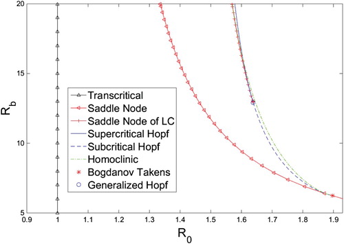There are four important ${\mathcal{R}}_b$ values which can be seen in the ${\mathcal{R}}_0$-${\mathcal{R}}_b$ bifurcation diagram in Figure 3. We work our way up from 0.

Figure 3. ${\mathcal{R}}_0$-${\mathcal{R}}_b$ bifurcation diagram for system (10(10) $\begin{array}{rl}\dot{I}& =\beta h\left(A\right)(1-I)I-\gamma I,\\ \dot{A}& =\frac{\alpha I(1-A)A^2}{{\delta }^2+A^2}-\xi A.\end{array}$(10) ) when $\delta =0.55$ created with the MATLAB MatCont package, and XPPAUT. The homoclinic curve was created using a bisection method.

From Theorem 4.3 the first critical ${\mathcal{R}}_b$ value is ${\mathcal{R}}_b^1=2/\left(1+\sqrt{1+1/{\delta }^2}\right).$ When ${\mathcal{R}}_b<{\mathcal{R}}_b^1$ behaviour is unable to invade, and our system is qualitatively similar to a classical SIS model. The DFE is globally stable when ${\mathcal{R}}_0<1$, and when ${\mathcal{R}}_0>1$ the endemic equilibrium exists in Ω and is stable. There are no other fixed points or cycles.

The second important ${\mathcal{R}}_b$ value occurs at a Bogdanov Takens (BT) point. The ${\mathcal{R}}_b$ value of this point will be denoted as ${\mathcal{R}}_b^2$. Varying ${\mathcal{R}}_0$ while ${\mathcal{R}}_b^2>{\mathcal{R}}_b>{\mathcal{R}}_b^1$ allows behaviour to invade. After the transcritical bifurcation creates the locally stable endemic point, ${\mathcal{R}}_0$ crosses $1/\left(1-2\delta \sqrt{1/{\mathcal{R}}_b+(1/{\mathcal{R}}_b{)}^2}\right)$ causing the system to undergo a saddle-node bifurcation creating a stable fixed point (13(13) $(I,A)=(I_{+},A_{+}),$(13) ) and a saddle (14(14) $(I,A)=(I_{-},A_{-}).$(14) ). The stable manifold of the saddle separates the basins of attraction of the two stable equilibria. In this parameter region the coexistence point of the complex contagion model is locally but not globally stable. This is in contrast with the simple contagion model, where (9(9) $(I,A)=(I^{\ast },A^{\ast })\mathrm{when}{\mathcal{R}}_0\ge \frac{{\mathcal{R}}_b}{{\mathcal{R}}_b-1}\ge 0.$(9) ) is globally stable, provided ${\mathcal{R}}_0$ is sufficiently large. An ${\mathcal{R}}_0$ bifurcation diagram for this ${\mathcal{R}}_b$ regime can be seen in Figure 5.

Figure 4. Cartoon of the ${\mathcal{R}}_0$-${\mathcal{R}}_b$ bifurcation diagram for system (10(10) $\begin{array}{rl}\dot{I}& =\beta h\left(A\right)(1-I)I-\gamma I,\\ \dot{A}& =\frac{\alpha I(1-A)A^2}{{\delta }^2+A^2}-\xi A.\end{array}$(10) ) when $\delta =0.55$. The bifurcation curves break the parameter space into seven distinct regions. Brief descriptions of these regions can be found in Table 2.

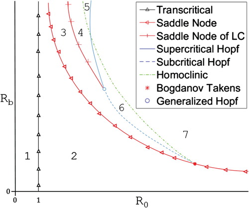
Figure 5. ${\mathcal{R}}_0$ bifurcation diagram for system (10(10) $\begin{array}{rl}\dot{I}& =\beta h\left(A\right)(1-I)I-\gamma I,\\ \dot{A}& =\frac{\alpha I(1-A)A^2}{{\delta }^2+A^2}-\xi A.\end{array}$(10) ) with $\delta =0.55$ and ${\mathcal{R}}_b=6$, which is in $({\mathcal{R}}_b^1,{\mathcal{R}}_b^2)$. Solid curves are stable fixed points, and dashed curves are unstable fixed points. Figure created with MATLAB and XPPAUT.

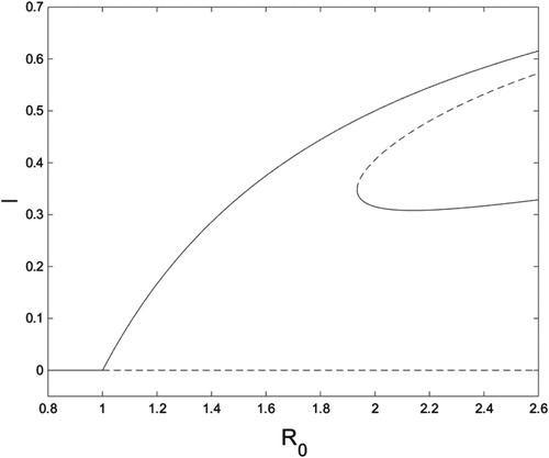
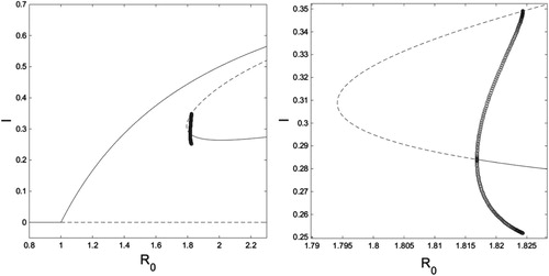
Above the BT point a generalized Hopf (GH) point occurs. The ${\mathcal{R}}_b$ value of the GH point is denoted ${\mathcal{R}}_b^3$. Increasing ${\mathcal{R}}_0$ while ${\mathcal{R}}_b\in ({\mathcal{R}}_b^2,{\mathcal{R}}_b^3)$ shows system (10(10) $\begin{array}{rl}\dot{I}& =\beta h\left(A\right)(1-I)I-\gamma I,\\ \dot{A}& =\frac{\alpha I(1-A)A^2}{{\delta }^2+A^2}-\xi A.\end{array}$(10) ) departs from system (5(5) $\begin{array}{rl}\dot{I}& =\beta h\left(A\right)(1-I)I-\gamma I\\ \dot{A}& =\alpha I(1-A)A-\xi A.\end{array}$(5) ) even further. In this interval the coexistence points (13(13) $(I,A)=(I_{+},A_{+}),$(13) ) and (14(14) $(I,A)=(I_{-},A_{-}).$(14) ) created through the saddle-node bifurcation are initially both unstable. As ${\mathcal{R}}_0$ increases the system undergoes a subcritical Hopf bifurcation, corresponding to (13(13) $(I,A)=(I_{+},A_{+}),$(13) ) becoming locally stable and the creation of an unstable limit cycle surrounding (13(13) $(I,A)=(I_{+},A_{+}),$(13) ). Continuing to increase ${\mathcal{R}}_0$ causes the unstable cycle to be destroyed through a homoclinic bifurcation, leaving a phase plane with the two stable fixed points separated by the stable manifold of the saddle, (14(14) $(I,A)=(I_{-},A_{-}).$(14) ), together with the unstable DFE. These transitions can be seen in Figure 6.

Figure 6. On the left is an ${\mathcal{R}}_0$ bifurcation diagram for system (10(10) $\begin{array}{rl}\dot{I}& =\beta h\left(A\right)(1-I)I-\gamma I,\\ \dot{A}& =\frac{\alpha I(1-A)A^2}{{\delta }^2+A^2}-\xi A.\end{array}$(10) ) with $\delta =0.55$ and ${\mathcal{R}}_b=7$, which is in $({\mathcal{R}}_b^2,{\mathcal{R}}_b^3)$. On the right is a close-up of the region where limit cycles occur. Solid curves are stable fixed points, dashed curves are unstable fixed points, and open circles are the minimum and maximum values of an unstable limit cycle. Figure created with MATLAB and XPPAUT.

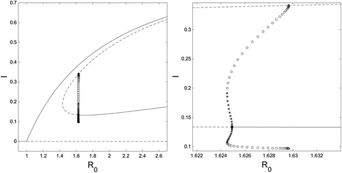
Above the GH point is the final important ${\mathcal{R}}_b$ value, ${\mathcal{R}}_b^4$. At ${\mathcal{R}}_b^4$ the ${\mathcal{R}}_0$-${\mathcal{R}}_b$ Hopf and homoclinic curves intersect. For ${\mathcal{R}}_b^4>{\mathcal{R}}_b>{\mathcal{R}}_b^3$ the saddle-node bifurcation again generates the unstable points (13(13) $(I,A)=(I_{+},A_{+}),$(13) ) and (14(14) $(I,A)=(I_{-},A_{-}).$(14) ). However, now as we increase ${\mathcal{R}}_0$ a saddle-node bifurcation of limit cycles occurs, creating both a stable and unstable limit cycle. Here the unstable limit cycle surrounds the stable limit cycle which circles (13(13) $(I,A)=(I_{+},A_{+}),$(13) ). Further raising ${\mathcal{R}}_0$ causes the stable cycle to shrink into (13(13) $(I,A)=(I_{+},A_{+}),$(13) ) until a supercritical Hopf bifurcation occurs and (13(13) $(I,A)=(I_{+},A_{+}),$(13) ) becomes a stable node. While this is occurring the unstable cycle grows until it is destroyed through a homoclinic bifurcation involving (14(14) $(I,A)=(I_{-},A_{-}).$(14) ) at an ${\mathcal{R}}_0$ value greater than the Hopf bifurcation value. Again we are left with two stable fixed points separated by the stable manifold of (14(14) $(I,A)=(I_{-},A_{-}).$(14) ) along with the DFE. These bifurcations can be examined in Figure 7.

Figure 7. On the left is an ${\mathcal{R}}_0$ bifurcation diagram for system (10(10) $\begin{array}{rl}\dot{I}& =\beta h\left(A\right)(1-I)I-\gamma I,\\ \dot{A}& =\frac{\alpha I(1-A)A^2}{{\delta }^2+A^2}-\xi A.\end{array}$(10) ) with $\delta =0.55$ and ${\mathcal{R}}_b=14$, which is in $({\mathcal{R}}_b^3,{\mathcal{R}}_b^4)$. On the right is a close-up of the region where limit cycles occur. Solid curves are stable fixed points, dashed curves are unstable fixed points, and open circles are the minimum and maximum values of an unstable limit cycle, and closed stars are the minimum and maximum values of a stable LC. Figure created with MATLAB and XPPAUT.

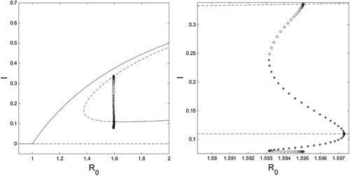
The only difference between the regions $({\mathcal{R}}_b^4,\mathrm{\infty })$ and $({\mathcal{R}}_b^3,{\mathcal{R}}_b^4)$ is the order of the supercritical Hopf and homoclinic bifurcations. In $({\mathcal{R}}_b^4,\mathrm{\infty })$, after the saddle-node bifurcation of limit cycles first the unstable cycle is destroyed through the homoclinic, and the stable limit cycle and endemic point are separated by the stable manifold of (14(14) $(I,A)=(I_{-},A_{-}).$(14) ). As ${\mathcal{R}}_0$ increases the stable cycle shrinks until it is absorbed by (13(13) $(I,A)=(I_{+},A_{+}),$(13) ) through a supercritical Hopf. Beyond this bifurcation the phase plane is made of two stable fixed points separated by the stable manifold of (14(14) $(I,A)=(I_{-},A_{-}).$(14) ), as well as the DFE. The difference can be explored by comparing Figures 7 and 8.

Figure 8. On the left is an ${\mathcal{R}}_0$ bifurcation diagram for system (10(10) $\begin{array}{rl}\dot{I}& =\beta h\left(A\right)(1-I)I-\gamma I,\\ \dot{A}& =\frac{\alpha I(1-A)A^2}{{\delta }^2+A^2}-\xi A.\end{array}$(10) ) with $\delta =0.55$ and ${\mathcal{R}}_b=17$, which is in $({\mathcal{R}}_b^4,\mathrm{\infty })$. On the right is a close-up of the region where limit cycles occur. Solid curves are stable fixed points, dashed curves are unstable fixed points, and open circles are the minimum and maximum values of an unstable limit cycle, and closed stars are the minimum and maximum values of a stable LC. Figure created with MATLAB and XPPAUT.

The above dynamical regions can be visually explored in a ${\mathcal{R}}_0$ -${\mathcal{R}}_b$ bifurcation diagram that is presented in Figures 3 and 4. A corresponding summary table of all the dynamics discussed is presented in Table 2.

Table 2. Steady state stability classification table for system (10(10) $\begin{array}{rl}\dot{I}& =\beta h\left(A\right)(1-I)I-\gamma I,\\ \dot{A}& =\frac{\alpha I(1-A)A^2}{{\delta }^2+A^2}-\xi A.\end{array}$(10) ) in each of the regions shown in Figures 4 and 10. LC means limit cycle and DNE means does not exist.

		Steady states
		DFE	Endemic	Point (13(13) $(I,A)=(I_{+},A_{+}),$(13) )	Point (14(14) $(I,A)=(I_{-},A_{-}).$(14) )	Unstable LC	Stable LC
	1	Globally stable	DNE	DNE	DNE	DNE	DNE
	2	Saddle	Globally stable	DNE	DNE	DNE	DNE
Region	3	Saddle	Locally stable	Unstable	Saddle	DNE	DNE
	4	Saddle	Locally stable	Unstable	Saddle	Around stable LC	Around Point (13(13) $(I,A)=(I_{+},A_{+}),$(13) )
	5	Saddle	Locally stable	Unstable	Saddle	DNE	Around Point (13(13) $(I,A)=(I_{+},A_{+}),$(13) )
	6	Saddle	Locally stable	Locally stable	Saddle	Around Point (13(13) $(I,A)=(I_{+},A_{+}),$(13) )	DNE
	7	Saddle	Locally stable	Locally stable	Saddle	DNE	DNE

Also of interest is how ${\mathcal{R}}_b$ and the half-saturation threshold parameter, δ, interact. Below we present a brief numerical analysis of the δ-${\mathcal{R}}_b$ parameter space when ${\mathcal{R}}_0$ is fixed at 1.6.

Varying δ and ${\mathcal{R}}_b$ together while holding ${\mathcal{R}}_0$ fixed gives dynamics that are similar to the ${\mathcal{R}}_0$-${\mathcal{R}}_b$ case. ${\mathcal{R}}_b$ determines the dynamical changes as δ is varied. There are again four critical ${\mathcal{R}}_b$ values. In ascending order they are: a cusp point (occurring at $(0,0)$), a BT point, a GH point, and where the δ-${\mathcal{R}}_b$ homoclinic and Hopf curves cross. These critical ${\mathcal{R}}_b$ values give four intervals for ${\mathcal{R}}_b$ that determine what bifurcations occur as δ is decreased. In increasing order the dynamics these four intervals produce are qualitatively the same as in $({\mathcal{R}}_b^1,{\mathcal{R}}_b^2),({\mathcal{R}}_b^2,{\mathcal{R}}_b^3),({\mathcal{R}}_b^3,{\mathcal{R}}_b^4),$ and $({\mathcal{R}}_b^4,\mathrm{\infty })$. Bifurcation diagrams in the δ-${\mathcal{R}}_b$ plane are given in Figures 9 and 10. We omit one-parameter δ bifurcation curves in this scenario because they are qualitatively the same as Figures 5 – 8 with the x-axis flipped because the bifurcations here occur as δ is decreased.

Figure 9. δ - ${\mathcal{R}}_b$ bifurcation diagram for system (10(10) $\begin{array}{rl}\dot{I}& =\beta h\left(A\right)(1-I)I-\gamma I,\\ \dot{A}& =\frac{\alpha I(1-A)A^2}{{\delta }^2+A^2}-\xi A.\end{array}$(10) ) with ${\mathcal{R}}_0=1.6$ created with the MATLAB MatCont package, and XPPAUT. The homoclinic curve was created using a bisection method.

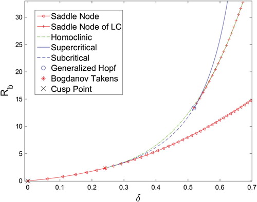
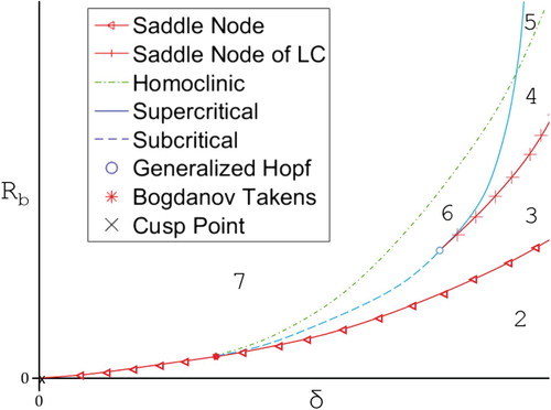
Figure 10. Cartoon of the $\delta -{\mathcal{R}}_b$ bifurcation diagram for system (10(10) $\begin{array}{rl}\dot{I}& =\beta h\left(A\right)(1-I)I-\gamma I,\\ \dot{A}& =\frac{\alpha I(1-A)A^2}{{\delta }^2+A^2}-\xi A.\end{array}$(10) ) with ${\mathcal{R}}_0=1.6$ showing the 6 regions the parameter space is broken into. Region descriptions can be found in Table 2.

As we can see the complex contagion model allows for much richer dynamics than simple contagion, with unforced periodic cycles, bistability, codimension 2 bifurcations, and the potential for codimension 3 bifurcations all supported.

5. Discussion

In this paper we have presented a family of models with the intention of examining how the mechanics of behavioural contagion can affect the coupled dynamics of behaviour and disease. The main finding of this work is that modelling behaviour transmission as a complex contagion can support much richer dynamics than treating it as a simple contagion in disease-behaviour coupled contagion models, including the possibility of both unforced oscillations and bistability.

These more complex dynamics of linked disease-social contagions may be useful for better understanding current disease propagation phenomena. For example, behaviour change has been implicated in the resurgence of syphilis in the United States [49], as well as increased gonorrhoea incidence rates [7]. Whether this is a precursor to sustained syphilis or gonorrhoea prevalence, or is instead part of a cycle involving changing behavioural practices and disease transmission, may depend in part on the mechanisms by which sexual norms, practices, and partner finding spreads between individuals and communities.

Although this model potentially provides insight into current disease phenomena it is important to carefully consider the assumptions underlying the modelling framework used here.

For example, a key assumption is that disease prevalence informs behavioural change. Empirical data on whether STI prevalence influences condom usage are equivocal [19]. Resolution of this issue would benefit from improved methods for collecting accurate data on condom usage [18].

Additionally, proper choices for $h\left(A\right)$ and $\ell \left(I\right)$ may very well differ between disease-behaviour pairings. In the work presented we made assumptions regarding the modulation factors, $\ell \left(I\right)$ and $h\left(A\right)$, that may not be true for all disease-behaviour pairings. For example, assumption (2) may depend on many factors including the disease and population being modelled. It is conceivable that ${\ell }^{\prime }\left(I\right)$ changes sign on $(0,1)$ when disease prevalence passes a threshold after which members of the population no longer perceive adopting the protective behaviour as beneficial. Such a situation could be relevant in settings where serosorting is widespread (e.g. condom usage decreasing for partnerships between HIV-positive individuals).

The different dynamics of the coupled contagion framework considered here also have implications for public health interventions targeting behaviour change. In system (5(5) $\begin{array}{rl}\dot{I}& =\beta h\left(A\right)(1-I)I-\gamma I\\ \dot{A}& =\alpha I(1-A)A-\xi A.\end{array}$(5) ) introducing any number of adopters has the potential to lower disease prevalence, provided that behaviour is sufficiently contagious. However, the bistability that can occur with system (10(10) $\begin{array}{rl}\dot{I}& =\beta h\left(A\right)(1-I)I-\gamma I,\\ \dot{A}& =\frac{\alpha I(1-A)A^2}{{\delta }^2+A^2}-\xi A.\end{array}$(10) ) makes lowering prevalence more difficult under complex behavioural contagion, and suggests that an initial high intensity campaign to enforce behaviour change may be needed to be effective. In addition, the possibility of oscillations with complex contagion behaviours could affect disease containment strategies as well. For instance, oscillations suggest that it could be critical to continue to invest in behavioural strategies despite low disease prevalence in order to prevent disease resurgence. Finally, interventions can target two different aspects of behaviour under complex contagion, namely the dissemination rate (α) and the half-saturation threshold (δ). It is possible that for some behaviours developing a media campaign that aims to lower the half-saturation threshold may be most effective, while targeting the adoption rate may be most beneficial for others.

The robustness of the dynamics observed above to model structure is an important question for future research on coupled contagion. For example, a robust feature is the finding that prevalence-based behaviours require the presence of a significantly infectious disease to spread. This finding held in both the simple and complex contagion settings considered here, where there existed regions for ${\mathcal{R}}_0$ in which behaviour is unable to invade the system. Similar findings are present in other studies of coupled contagion using compartmental [15] and static network models [21, 56].

Whether the qualitative dynamics observed in model (10(10) $\begin{array}{rl}\dot{I}& =\beta h\left(A\right)(1-I)I-\gamma I,\\ \dot{A}& =\frac{\alpha I(1-A)A^2}{{\delta }^2+A^2}-\xi A.\end{array}$(10) ) are also observed in other modelling frameworks is an area for future work. Given previous results on dynamics supported by nonlinear incidence functions [28, 34, 35], we expect similar qualitative dynamics when assumption (2) is relaxed and the model is extended to include sub-compartments. As discussed in Section 3, existing sub-compartmental models with simple behavioural contagion exhibit similar dynamics as system (5(5) $\begin{array}{rl}\dot{I}& =\beta h\left(A\right)(1-I)I-\gamma I\\ \dot{A}& =\alpha I(1-A)A-\xi A.\end{array}$(5) ), but formulation and analysis is required for a complex behavioural contagion model. Comparison of the dynamics found here with coupled complex contagion in the network setting is of interest as well. Of particular interest is the active field of epidemic spread on multiplex networks [4, 21, 58]. Our presented modelling framework could be expanded to a setting in which disease spreads over a layer modelling physical contacts while behaviour spreads over a second layer modelling the medium by which behaviour spreads (be it through physical or virtual interaction) among the same nodes [21].

An important question is how the specific choice of behavioural incidence function, g, affects system dynamics. Our choice here of a Hill function is as an example of an incidence function which changes concavity from up to down on the biologically relevant domain. This is meant to correspond to the initial acceleration and subsequent saturation of the force of infection corresponding to complex contagion. For many epidemiological models [28, 34, 35], incidence functions of this form support rich dynamics, in contrast with the simple dynamics associated with incidence functions that are concave down throughout, suggesting that the general finding of complex behavioural contagion supporting complex dynamics may be robust. However, definitive proof of this hypothesis requires further investigation.

The details of how behaviour impacts disease transmission are likewise important to further study. Other studies have explicitly modelled the effects of disease on behaviour, for example via rewiring in adaptive network models [22–24, 32, 45, 50, 52] and game theoretic models [25, 42], and have found that behavioural-driven oscillations are possible.

Nonlinear incidence functions have long been known to produce interesting bifurcations and oscillations in disease models that do not explicitly include behaviour [28, 34, 35]. The finding here of rich dynamics by itself is thus not novel. The point that we wish to make is that careful consideration of behavioural contagion type when incorporating behaviour as a contagious process into epidemic models may be important, as differing contagion types can lead to dramatically different dynamics. This can have important practical considerations for preventative behaviours recommended by public health authorities. Preventative behaviours may spread in different manners, and thus it is crucial to understand both the theoretical and practical implications of different behavioural contagion types.

Acknowledgements

The authors declare only academically motivated interest, and the funding sources played no role in any of the research presented above.

Disclosure statement

No potential conflict of interest was reported by the authors.

ORCID

Matthew Osborne http://orcid.org/0000-0001-5217-0392

Additional information

Funding

This work was supported by the National Science Foundation [grant number OCE-1115881], and the Mathematical Biosciences Institute [grant number DMS-0931642]. MTO was supported by a Rhodus Graduate Fellowship from the Ohio State University's Department of Mathematics. XW acknowledges support from the Simons Foundation [grant number #317047] and a long-term visitor fellowship from the Mathematical Biosciences Institute.

References

- C.T. Bauch, A.P. Galvani, Social and biological contagions. Science (New York, NY) 342 (2013), pp. 47. doi: 10.1126/science.1244492
- D. Bernoulli, Essai d'une nouvelle analyse de la mortalité causée par la petite vérole et des avantages de l'inoculation pour la prévenir, Histoire de l'Acad. Roy. Sci.(Paris) avec Mém. des Math. et Phys. and Mém 1 (1760), pp. 1–45.
- D. Bernoulli and S. Blower, An attempt at a new analysis of the mortality caused by smallpox and of the advantages of inoculation to prevent it, Rev. Med. Virol. 14 (2004), pp. 275–288. doi: 10.1002/rmv.443
- S. Boccaletti, G. Bianconi, R. Criado, C.I. Del Genio, J. Gómez-Gardenes, M. Romance, I. Sendina-Nadal, Z. Wang, and M. Zanin, The structure and dynamics of multilayer networks, Phys. Rep. 544 (2014), pp. 1–122. doi: 10.1016/j.physrep.2014.07.001
- W. Cates Jr and K.M. Stone, Family planning, sexually transmitted diseases and contraceptive choice: A literature update–part I, Fam. Plann. Perspectives 24 (1992), pp. 75–84. doi: 10.2307/2135469
- D. Centola, The spread of behavior in an online social network experiment, Science 329 (2010), pp. 1194–1197. doi: 10.1126/science.1185231
- Y. Choudhri, J. Miller, J. Sandhu, A. Leon, and J. Aho, Infectious and congenital syphilis in canada, 2010–2015, Sex. Trans. Infect. 44 (2018), pp. 43.
- N.A. Christakis and J.H. Fowler, The spread of obesity in a large social network over 32 years, New Engl. J. Med. 2007 (2007), pp. 370–379. doi: 10.1056/NEJMsa066082
- O. Diekmann, J.A.P. Heesterbeek, and J.A. Metz, On the definition and the computation of the basic reproduction ratio R0 in models for infectious diseases in heterogeneous populations, J. Math. Biol. 28 (1990), pp. 365–382. doi: 10.1007/BF00178324
- M.C. Eisenberg, Z. Shuai, J.H. Tien, and P. Van den Driessche, A cholera model in a patchy environment with water and human movement, Math. Biosci. 246 (2013), pp. 105–112. doi: 10.1016/j.mbs.2013.08.003
- J.M. Epstein, J. Parker, D. Cummings, and R.A. Hammond, Coupled contagion dynamics of fear and disease: Mathematical and computational explorations, PLoS One 3 (2008), pp. e3955. doi: 10.1371/journal.pone.0003955
- J.D. Fortenberry, W. Tu, J. Harezlak, B.P. Katz, and D.P. Orr, Condom use as a function of time in new and established adolescent sexual relationships, Am. J. Public Health 92 (2002), pp. 211–213. doi: 10.2105/AJPH.92.2.211
- F. Fu, N.A. Christakis, and J.H. Fowler, Dueling biological and social contagions, Sci. Rep. 7 (2017), pp. 43634. doi: 10.1038/srep43634
- S. Funk, S. Bansal, C.T. Bauch, K.T. Eames, W.J. Edmunds, A.P. Galvani, and P. Klepac, Nine challenges in incorporating the dynamics of behaviour in infectious diseases models, Epidemics 10 (2015), pp. 21–25. doi: 10.1016/j.epidem.2014.09.005
- S. Funk, E. Gilad, and V. Jansen, Endemic disease, awareness, and local behavioural response, J. Theor. Biol. 264 (2010), pp. 501–509. doi: 10.1016/j.jtbi.2010.02.032
- S. Funk, E. Gilad, C. Watkins, and V.A. Jansen, The spread of awareness and its impact on epidemic outbreaks, Proc. Natl. Acad. Sci. 106 (2009), pp. 6872–6877. doi: 10.1073/pnas.0810762106
- S. Funk, M. Salathé, and V.A.A. Jansen, Modelling the influence of human behaviour on the spread of infectious diseases: A review, J. R. Soc. Interface 7 (2010), pp. 1247–1256. doi: 10.1098/rsif.2010.0142
- M.F. Gallo, M.J. Steiner, M.M. Hobbs, L. Warner, D.J. Jamieson, and M. Macaluso, Biological markers of sexual activity: Tools for improving measurement in HIV/sexually transmitted infection prevention research, Sex. Trans. Dis. 40 (2013), pp. 447–452. doi: 10.1097/OLQ.0b013e31828b2f77
- M. Gerrard, F.X. Gibbons, and B.J. Bushman, Relation between perceived vulnerability to HIV and precautionary sexual behavior, Psychol. Bull. 119 (1996), pp. 390. doi: 10.1037/0033-2909.119.3.390
- W. Goffman and V.A. Newill, Generalization of epidemic theory: An application to the transmission of ideas, Nature 204 (1964), pp. 225–228. doi: 10.1038/204225a0
- C. Granell, S. Gómez, and A. Arenas, Dynamical interplay between awareness and epidemic spreading in multiplex networks, Phys. Rev. Lett. 111 (2013), pp. 128701. doi: 10.1103/PhysRevLett.111.128701
- T. Gross and B. Blasius, Adaptive coevolutionary networks: A review, J. R. Soc. Interface 5 (2008), pp. 259–271. doi: 10.1098/rsif.2007.1229
- T. Gross, C.J.D. D'Lima, and B. Blasius, Epidemic dynamics on an adaptive network, Phys. Rev. Lett. 96 (2006), pp. 208701. doi: 10.1103/PhysRevLett.96.208701
- T. Gross and I.G. Kevrekidis, Robust oscillations in SIS epidemics on adaptive networks: Coarse graining by automated moment closure, EPL (Europhys. Lett.) 82 (2008), pp. 38004. doi: 10.1209/0295-5075/82/38004
- M.A. Hayashi and M.C. Eisenberg, Effects of adaptive protective behavior on the dynamics of sexually transmitted infections, J. Theor. Biol. 388 (2016), pp. 119–130. doi: 10.1016/j.jtbi.2015.08.022
- G.M. Herek, E.K. Glunt, An Epidemic of Stigma: Public Reactions to AIDS. vol. 43, American Psychological Association, Washington D.C., 1988
- H. Hethcote and J. Yorke, Gonorrhea Transmission Dynamics and Control (Lecture Notes in Biomathematics 56), Springer-Verlag, New York, 1984.
- H.W. Hethcote and P. Van Den Driessche, Some epidemiological models with nonlinear incidence, J. Math. Biol. 29 (1991), pp. 271–287. doi: 10.1007/BF00160539
- K.K. Holmes, R. Levine, and M. Weaver, Effectiveness of condoms in preventing sexually transmitted infections, Bull. World Health Organ. 82 (2004), pp. 454–461.
- W.O. Kermack and A.G. McKendrick, A contribution to the mathematical theory of epidemics, in Proceedings of the Royal Society of London A: Mathematical, Physical and Engineering Sciences, vol. 115, The Royal Society, 1927, pp. 700–721
- S.B. Kinsman, D. Romer, F.F. Furstenberg, and D.F. Schwarz, Early sexual initiation: The role of peer norms, Pediatrics 102 (1998), pp. 1185–1192. doi: 10.1542/peds.102.5.1185
- I.Z. Kiss, L. Berthouze, T.J. Taylor, and P.L. Simon, Modelling approaches for simple dynamic networks and applications to disease transmission models, in Proc. R. Soc. A, vol. 468, The Royal Society, 2012, pp. 1332–1355
- I.Z. Kiss, J. Cassell, M. Recker, and P.L. Simon, The impact of information transmission on epidemic outbreaks, Math. Biosci. 225 (2010), pp. 1–10. doi: 10.1016/j.mbs.2009.11.009
- W.-m. Liu, H.W. Hethcote, and S.A. Levin, Dynamical behavior of epidemiological models with nonlinear incidence rates, J. Math. Biol. 25 (1987), pp. 359–380. doi: 10.1007/BF00277162
- W.-m. Liu, S.A. Levin, and Y. Iwasa, Influence of nonlinear incidence rates upon the behavior of SIRS epidemiological models, J. Math. Biol. 23 (1986), pp. 187–204. doi: 10.1007/BF00276956
- A. Lynch, Thought contagion as abstract evolution, J. Ideas 2 (1991), pp. 3–10.
- J.M. Mann, AIDS in the World, Harvard University Press, Cambridge, MA, 1992.
- B. Mønsted, P. Sapieżyński, E. Ferrara, and S. Lehmann, Evidence of complex contagion of information in social media: An experiment using twitter bots, PloS One 12 (2017), pp. e0184148. doi: 10.1371/journal.pone.0184148
- J.T. Parsons, P.N. Halkitis, D. Bimbi, and T. Borkowski, Perceptions of the benefits and costs associated with condom use and unprotected sex among late adolescent college students, J. Adolesc. 23 (2000), pp. 377–391. doi: 10.1006/jado.2000.0326
- N. Perra, D. Balcan, B. Gonçalves, and A. Vespignani, Towards a characterization of behavior-disease models, PloS One 6 (2011), pp. e23084. doi: 10.1371/journal.pone.0023084
- J.H. Pleck, F.L. Sonenstein, and L.C. Ku, Adolescent males' condom use: Relationships between perceived cost-benefits and consistency, J. Marriage Fam. 53 (1991), pp. 733–745. doi: 10.2307/352747
- T.C. Reluga, C.T. Bauch, and A.P. Galvani, Evolving public perceptions and stability in vaccine uptake, Math. Biosci. 204 (2006), pp. 185–198. doi: 10.1016/j.mbs.2006.08.015
- D. Romer, M. Black, I. Ricardo, S. Feigelman, L. Kaljee, J. Galbraith, R. Nesbit, R.C. Hornik, and B. Stanton, Social influences on the sexual behavior of youth at risk for HIV exposure, Am. J. Public Health 84 (1994), pp. 977–985. doi: 10.2105/AJPH.84.6.977
- F.D. Sahneh, F.N. Chowdhury, and C.M. Scoglio, On the existence of a threshold for preventive behavioral responses to suppress epidemic spreading, Sci. Rep. 2 (2012), pp. 632. doi: 10.1038/srep00632
- L.B. Shaw and I.B. Schwartz, Fluctuating epidemics on adaptive networks, Phys. Rev. E 77 (2008), pp. 066101. doi: 10.1103/PhysRevE.77.066101
- P. Sheeran, C. Abraham, and S. Orbell, Psychosocial correlates of heterosexual condom use: A meta-analysis, Psychol. Bull. 125 (1999), pp. 90. doi: 10.1037/0033-2909.125.1.90
- J. Snow, On the Mode of Communication of Cholera, John Churchill, New Burlington Street. London, 1855.
- D.A. Sprague and T. House, Evidence for complex contagion models of social contagion from observational data, PloS one 12 (2017), pp. e0180802. doi: 10.1371/journal.pone.0180802
- L.V. Stamm and B. Mudrak, Old foes, new challenges: Syphilis, cholera and TB, Future Microbiol. 8 (2013), pp. 177–189. doi: 10.2217/fmb.12.148
- A. Szabó-Solticzky, L. Berthouze, I.Z. Kiss, and P.L. Simon, Oscillating epidemics in a dynamic network model: Stochastic and mean-field analysis, J. Math. Biol. 72 (2016), pp. 1153–1176. doi: 10.1007/s00285-015-0902-3
- S.M. Tracht, S.Y. DelValle, and J.M. Hyman, Mathematical modelling of the effectiveness of facemasks in reducing the spread of novel influenza A (H1N1), PloS One 5 (2010), pp. e9018. doi: 10.1371/journal.pone.0009018
- I. Tunc and L.B. Shaw, Effects of community structure on epidemic spread in an adaptive network, Phys. Rev. E 90 (2014), pp. 022801. doi: 10.1103/PhysRevE.90.022801
- P. Van den Driessche and J. Watmough, Reproduction numbers and sub-threshold endemic equilibria for compartmental models of disease transmission, Math. Biosci. 180 (2002), pp. 29–48. doi: 10.1016/S0025-5564(02)00108-6
- Z. Wang, M.A. Andrews, Z.-X. Wu, L. Wang, and C.T. Bauch, Coupled disease–behavior dynamics on complex networks: A review, Phys. Life Rev. 15 (2015), pp. 1–29. doi: 10.1016/j.plrev.2015.07.006
- W. Wang, Q.-H. Liu, S.-M. Cai, M. Tang, L.A. Braunstein, and H.E. Stanley, Suppressing disease spreading by using information diffusion on multiplex networks, Sci. Rep. 6 (2016), pp. 29259. doi: 10.1038/srep29259
- W. Wang, M. Tang, H. Yang, Y. Do, Y.-C. Lai, and G. Lee, Asymmetrically interacting spreading dynamics on complex layered networks, Sci. Rep. 4 (2014), pp. 5097. doi: 10.1038/srep05097
- Q. Wu, X. Fu, M. Small, and X.-J. Xu, The impact of awareness on epidemic spreading in networks, Chaos: Interdiscip. J. Nonlinear Sci. 22 (2012), pp. 013101.
- D. Zhao, L. Li, H. Peng, Q. Luo, and Y. Yang, Multiple routes transmitted epidemics on multiplex networks, Phys. Lett. A 378 (2014), pp. 770–776. doi: 10.1016/j.physleta.2014.01.014