Weather-driven malaria transmission model with gonotrophic and sporogonic cycles

ABSTRACT

Malaria is mainly a tropical disease and its transmission cycle is heavily influenced by environment: The life-cycles of the Anopheles mosquito vector and Plasmodium parasite are both strongly affected by ambient temperature, while suitable aquatic habitat is necessary for immature mosquito development. Therefore, how global warming may affect malaria burden is an active question, and we develop a new ordinary differential equations-based malaria transmission model that explicitly considers the temperature-dependent Anopheles gonotrophic and Plasmodium sporogonic cycles. Mosquito dynamics are coupled to infection among a human population with symptomatic and asymptomatic disease carriers, as well as temporary immunity. We also explore the effect of incorporating diurnal temperature variations upon transmission. Rigorous analysis of the model show that the non-trivial disease-free equilibrium is locally-asymptotically stable when the associated reproduction number is less than unity (this equilibrium is globally-asymptotically for a special case with no density-dependent larval and disease-induced host mortality). Numerical simulations of the model, for the case where the ambient temperature is held constant, suggest a nonlinear, hyperbolic relationship between the reproduction number and clinical malaria burden. Moreover, malaria burden peaks at 29.5 ${}^{\mathrm{o}}$C when daily ambient temperature is held constant, but this peak decreases with increasing daily temperature variation, to about 23–25 ${}^{\mathrm{o}}$C. Malaria burden also varies nonlinearly with temperature, such that small temperature changes influent disease mainly at marginal temperatures, suggesting that in areas where malaria is highly endemic, any response to global warming may be highly nonlinear and most typically minimal, while in areas of more marginal malaria potential (such as the East African highlands), increasing temperatures may translate nearly linearly into increased disease potential. Finally, we observe that while explicitly modelling the stages of the Plasmodium sporogonic cycle is essential, explicitly including the stages of the Anopheles gonotrophic cycle is of minimal importance.

KEYWORDS:

• Malaria
• gonotrophic cycle
• sporogonic cycle
• reproduction number
• thermal-response
• weather-driven model

1. Introduction

Malaria, one of the world's oldest vector-borne diseases (VBD) and caused by evolutionarily ancient Plasmodium parasites, has burdened humanity for many tens of thousands of years, but it was probably not until about 10,000 years ago that the most virulent form of the disease, P. falciparum, arose in proto-agricultural Africa [17,52] to plague humanity to this day. Nearly half a million deaths are still attributable to malaria annually [99], with over 90% of mortality due to P. falciparum in Africa, and, moveover, most fatal cases occur in children under the age of five. Despite the existence of effective preventative measures and treatment, malaria remains endemic in 91 countries, with the morbidity and mortality heavily concentrated in resource-poor areas of sub-Saharan Africa [99].

Malaria is one of the earliest diseases subject to mathematical inquiry, beginning with the work of Sir Ronald Ross (who discovered the malaria lifecycle) in the early 1900s [84], and its extensions in the early 1950s by the highly influential British malariologist George Macdonald [54]. Since these seminal works, numerous mathematical models have been introduced to study malaria transmission (a very partial reference list includes [1,21,26,33,49,68], see also [79] for a review of malaria models). More recently, numerous authors (e.g., [4,22,31,32,69,73,75,102]) have turned to modelling to quantify the impact of weather and climate on malaria transmission, mainly focussing on temperature and rainfall, and how anthropogenic climate change might be expected to affect (potential) disease burden, especially in tropical Africa. Climate is expected to influence malaria because both vector and parasite have highly temperature- and rainfall-dependent lifecycles, as now briefly reviewed.

The life-cycle of the Anopheles mosquito consists of adult and aquatic juvenile stages. At the aquatic stage, immature mosquitoes develop from eggs, through four larval instar stages, and finally into pupae that hatch into adults. Both survival and development at the aquatic stage are temperature-dependent, with survival peaking around 20${}^{\circ }$C [11], and developmental rates increasing with temperature up to at least 30${}^{\circ }$C [10]. Furthermore, the existence of aquatic habitats depends upon appropriate land cover and (away from permanent standing or running water), sufficient rainfall to support the small, ephemeral pools often preferred by malaria mosquitoes, such as An. gambiae [60].

At the adult stage, the female mosquito lifecycle is defined by the gonotrophic cycle (Greek “offspring feeding”), whereby the female mosquito takes mammalian bloodmeals to nourish egg development and then deposits them on the surface of appropriate waters, and classically divided into three stages [25]:

Stage I:	Search for suitable host and the taking of a bloodmeal.
Stage II:	Digestion of blood meal and egg maturation (this process is highly temperature dependent).
Stage III:	Search for, and oviposition into, a suitable body of water.

Much like immature development, the rate at which Stage II (egg development) progresses depends upon ambient temperature, increasing up to around 30${}^{\circ }$C, levelling off, and possibly sharply declining at very high temperature [44]. Survival, likewise, peaks in the mid-20s (${}^{\circ }$C), and is impaired at both low and high temperatures. The Anopheles lifecycle is depicted schematically in Figure 1.

Figure 1. Anopheles mosquito lifecycle. Immature mosquitoes pass through aquatic egg, larvae, and pupae stages, with the actively feeding larvae divided into four instar stages. Adult female mosquitoes pass through the gonotrophic cycle, by which blood meals nourish the development of new eggs.

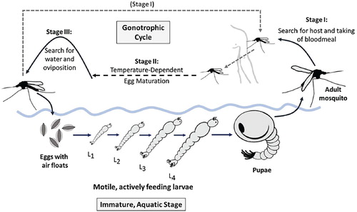
Malaria transmission occurs when, during Stage I of the gonotrophic cycle, a susceptible mosquito takes a bloodmeal from an infectious host with Plasmodium gametocytes in their red blood cells. This initiates the sporogonic (or extrinsic) cycle, by which the gametocytes undergo several transformations to penetrate the wall of the mosquito midgut, eventually yielding sporozoites that infest the mosquito's salivary glands, where they can infect the victim of the anopheline's next bloodmeal. As with other developmental processes, the sporogonic cycle also generally progresses more rapidly at higher temperatures [25].

As the extrinsic incubation period can be similar to the average life expectancy of the female Anopheles mosquito [14,25,67,74], we see how suboptimal temperatures can severely impair malaria transmission potential via a decrease in adult survival, but also via impaired immature survival, a decrease in the number of larval that successfully become adults, a decrease in the biting rate (via an increase in the gonotrophic cycle duration) and by lengthening the sporogonic cycle such that it rarely completes within the lifetime of the host mosquito. Indeed, the consideration of the delay from initial mosquito infection to infectiousness was a key factor in Macdonald's malaria model, with the model suggesting that interruption of the sporogonic cycle is the main benefit of insecticidal control measures that reduce adult survival [54].

It follows that anthropogenic climate change may alter the (potential) distribution of malarial disease, and this has been the focus of many mechanistic (or process-based) malaria transmission models. Overall, such models have reached divergent conclusions, with some predicting a large expansion in the continental land area suitable for transmission [19,57,93] and in the number of people at risk of malaria [57,76,77], while others predict only modest poleward (and altitudinal) shifts in the burden of disease, with little net effect [36,39,83]. In other words, the current related debate within the ecology community is on poleward-expansion of malaria from tropical latitudes vs. poleward-shift-with-no-net-expansion in malaria cases. Similarly, malaria burden may expand into equatorial highland areas, such as those of Eastern Africa, with uncertain changes at lower altitude [15,36,45,46,76,83]; several recent works suggest possible increases in disease potential in Central and Eastern Africa, but little change in Western Africa [32,85,101]. Additionally, models differ regarding the expected optimum temperature for transmission [61,69]. In particular, Mordecai et al. [61] showed that earlier models which use monotonic functions for the vector and parasite temperature-dependent vital rates, may have over-estimated the optimal temperature range for malaria transmission. Furthermore, most of the aforementioned modelling studies used constant or mean monthly temperature in their formulation. Recent studies have shown that the incorporation of daily (diurnal) temperature fluctuations in the model may also affect predictions [12,13,74].

The sporogonic and gonotrophic cycles are clearly central to malaria transmission dynamics and should, we argue, be explicitly addressed in any mathematical model for the process. To explicitly account for the effect of the gonotrophic cycle on malaria transmission, Ngonghala et al. [65] considered a mathematical model for the dynamics of malaria transmission that integrates the gonotrophic cycle of the adult female mosquitoes and its interaction with the human population (their model was an extension of the mosquito population ecology model developed by Ngwa [64, to incorporate disease dynamics in both the human and adult vector populations). The model in Ngonghala et al. [65], which considered infection of the female Anopheles mosquitoes to result in infectiousness immediately after interaction with an infected human, was later extended to include the exposed class of mosquitoes, thereby explicitly accounting for the effect of the duration of Plasmodium development in the vector [66]. As shown in the classical Macdonald's malaria model [54], the sporogonic cycle plays a profound role in the epidemiological effectiveness of malaria vectors and, consequently, on malaria incidence in human host populations. Hence, it is likely necessary to explicitly incorporate the duration of both the temperature-dependent gonotrophic and sporogony cycles in the transmitting vector in models for malaria transmission dynamics in populations.

We extend the previous autonomous (temperature-independent) models by Ngonghala et al. [65,66] to a non-autonomous (temperature-dependent) model with sporogony represented via the division of the adult female mosquito population into three classes (susceptible, exposed and infectious), while gonotrophy is modelled by additionally splitting the adult mosquito population into three classes corresponding to the gonotrophic stages discussed above (yielding a nine-compartment model for the dynamics of the adult female mosquitoes). Further, we model the immature mosquito lifecycle by including compartments for all major developmental stages (eggs, four larval instars, and pupae), and incorporate dependence on temperature at this stage as well. Finally, we incorporate disease transmission to vectors by asymptomatically-infectious humans, reduced malaria susceptibility in humans due to recovery from prior infection, the possibility of progression from a symptomatically-infected to asymptomatically-infected state, and the complete loss of partial immunity in humans.

The paper is organized as follows. The mathematical model for malaria transmission dynamics, incorporating gontrophic and sporogonic cycles in adult female mosquitoes and the variability in local weather (temperature) patterns, is presented in Section 2. The autonomous equivalent of the model, where the temperature-dependent parameters of the model are assumed to be constant, is analyzed in Section 3. Sensitivity analysis is also carried out in this section to determine the parameters that have the most influence on the disease dynamics. The full non-autonomous model is analyzed and simulated in Section 4.

2. Description and formulation of model

We extend the model of Ngonghala et al. [65], to a non-autonomous (temperature-dependent) model which includes all immature stages of mosquitoes (eggs, four larval instars and pupae), as well as an exposed class (to account for the delay to infectiousness in the Plasmodium sporogonic cycle) for each stage of the gonotrophic cycle of the adult female mosquitoes. In addition, we consider epidemiological features of malaria transmission such as disease transmission to mosquitoes by asymptomatically-infectious humans, reduced malaria susceptibility in humans due to recovery from prior malaria infection, the possibility of progression from a symptomatically infected to asymptomatically infected state, and the complete loss of partial immunity in humans.

2.1. State variables

The total human population at time t, $N_H\left(t\right)$, is divided into the sub-populations of wholly-susceptible humans ($S_H\left(t\right))$, susceptible humans with prior immunity due to past exposure and recovery from malaria infection ($W_H\left(t\right))$, exposed (infected but not yet infectious) humans without prior malaria immunity (i.e., exposed and malaria naive humans) ($E_{HN}\left(t\right))$, exposed humans with partial malaria immunity due to recovery from prior infection ($E_{HR}\left(t\right))$, symptomatic and infectious humans ($I_H\left(t\right))$, asymptomatic and infectious humans ($A_H\left(t\right))$ and recovered ($R_H\left(t\right))$ humans, so that $N_H\left(t\right)=S_H\left(t\right)+W_H\left(t\right)+E_{HN}\left(t\right)+E_{HR}\left(t\right)+I_H\left(t\right)+A_H\left(t\right)+R_H\left(t\right).$ The immature mosquito population at time t is divided into compartments for eggs ($E\left(t\right))$, four larval instar stages ($L_1\left(t\right),L_2\left(t\right),L_3\left(t\right),L_4\left(t\right))$, and pupae ($P\left(t\right)$). The adult female mosquito gonotrophic cycle is divided into three stages (as discussed in the Introduction): (I) temperature-independent host-seeking, (II) temperature-dependent bloodmeal digestion, and (III) temperature-independent oviposition. Vectors in Stages I, II and III at time t are denoted by $X\left(t\right)$, $Y\left(t\right)$ and $Z\left(t\right)$, respectively. With respect to Plasmodium infection and the sporogonic cycle, vectors in each gonotrophic stage is further subdivided into susceptible ($S_X\left(t\right),S_Y\left(t\right),S_Z\left(t\right)$), exposed ($E_X\left(t\right),E_Y\left(t\right),E_Z\left(t\right)$) and infected ($I_X\left(t\right),I_Y\left(t\right),I_Z\left(t\right)$) compartments. Thus, the total number of adult mosquitoes at time t, $N_M\left(t\right)$, is given as $N_M\left(t\right)=S_X\left(t\right)+E_X\left(t\right)+I_X\left(t\right)+S_Y\left(t\right)+E_Y\left(t\right)+I_Y\left(t\right)+S_Z\left(t\right)+E_Z\left(t\right)+I_Z\left(t\right).$ The equations for the dynamics of each of the major sub-components of the model are derived below.

2.2. Equations for dynamics of immature mosquitoes

Eggs are produced according to the logistic term, ${\psi }_E{\varphi }_Z(1-\frac{E}{K_E}{)}_{+}(S_Z+E_Z+I_Z),$ where ${\psi }_E$ is the number of eggs laid per oviposition, ${\varphi }_Z$ is the rate at which female mosquitoes transition from Stage III to Stage I of the gonotrophic cycle (i.e., the rate of oviposition for mosquitoes in Stage III) and $K_E$ is the environmental carrying capacity of eggs (the notation $r_{+}=max\{0,r\}$ is used to ensure the non-negativity of the logistic term). The equations for the dynamics of immature mosquitoes are given as (where T_W is water temperature): (1) $\begin{array}{rl}\frac{\mathrm{d}E}{\mathrm{d}t}& ={\psi }_E{\varphi }_Z{\left(1-\frac{E}{K_E}\right)}_{+}(S_Z+E_Z+I_Z)-[{\sigma }_E\left(T_W\right)+{\eta }_E+{\mu }_E]E,\\ \frac{\mathrm{d}{L}_1}{\mathrm{d}t}& ={\sigma }_E\left(T_W\right)E-[{\sigma }_{L_1}\left(T_W\right)+{\eta }_L+k_{L}L+{\mu }_L\left(T_W\right)]L_1,\\ \frac{\mathrm{d}{L}_j}{\mathrm{d}t}& ={\sigma }_{L_{(j-1)}}\left(T_W\right)L_{j-1}-[{\sigma }_{Lj}\left(T_W\right)+{\eta }_L+k_{L}L+{\mu }_L\left(T_W\right)]L_j,j=2,3,4,\\ \frac{\mathrm{d}P}{\mathrm{d}t}& ={\sigma }_{L_4}\left(T_W\right)L_4-[{\sigma }_P\left(T_W\right)+{\eta }_P+{\mu }_P]P.\end{array}$(1) The parameters ${\mu }_i\left(T_W\right)$ and ${\eta }_i$ (i=E, L, P) represent the temperature-dependent and temperature-independent death rates, respectively, for immature mosquitoes of type i, where the latter may be due to processes such as predation, anthropogenic vector control measures, etc. Density-dependent larval mortality occurs at a rate $k_{L}L$ (where $L=L_1+L_2+L_3+L_4$), although we generally set $k_L$ = 0 and consider the population to be limited only at the oviposition stage. Finally, ${\sigma }_E\left(T_W\right)$ is the temperature-dependent hatching rate of eggs into larvae, ${\sigma }_{Lj}\left(T_W\right)(j=1,2,3)$ is the temperature-dependent progression rate of larvae from instar stage j to stage j+1, and ${\sigma }_P\left(T_W\right)$ is the temperature-dependent rate at which pupae mature into adult mosquitoes.

2.3. Equations for dynamics of adult mosquitoes

It should be noted, first of all, that only mosquitoes in Stage I of the gonotrophic cycle (i.e., mosquitoes of type X in our formulation, regardless of infection status) will bite humans. That is, only mosquitoes in classes $S_X,E_X$ and $I_X$ bite humans. The fraction of these bites that potentially result in an infection is given as: ${\mathcal{G}}_H=\frac{I_H+A_H}{N_H}.$ That is, ${\mathcal{G}}_H$ is the proportion of infectious humans (both symptomatic and asymptomatic) in the community (for mathematical tractability, we do not distinguish the transmissibility of the two infectious classes). The equations for the dynamics of adult female mosquitoes are given by (where T_A is air/ambient temperature): (2) $\begin{array}{rl}\frac{\mathrm{d}{S}_X}{\mathrm{d}t}& =f{\sigma }_P\left(T_W\right)P+{\varphi }_Z{S}_Z-[b_H+{\eta }_M+{\mu }_M\left(T_A\right)]S_X,\\ \frac{\mathrm{d}{E}_X}{\mathrm{d}t}& ={\varphi }_Z{E}_Z-[b_H+{\kappa }_M\left(T_A\right)+{\eta }_M+{\mu }_M\left(T_A\right)]E_X,\\ \frac{\mathrm{d}{I}_X}{\mathrm{d}t}& ={\varphi }_Z{I}_Z+{\kappa }_M\left(T_A\right)E_X-[b_H+{\eta }_M+{\mu }_M\left(T_A\right)]I_X,\\ \frac{\mathrm{d}{S}_Y}{\mathrm{d}t}& =b_H(1-{\beta }_V){\mathcal{G}}_H{S}_X+b_H(1-{\mathcal{G}}_H)S_X-[{\theta }_Y\left(T_A\right)+{\eta }_M+{\mu }_M\left(T_A\right)]S_Y,\\ \frac{\mathrm{d}{E}_Y}{\mathrm{d}t}& =b_H{\beta }_V{\mathcal{G}}_H{S}_X+b_H{E}_X-[{\theta }_Y\left(T_A\right)+{\kappa }_M\left(T_A\right)+{\eta }_M+{\mu }_M\left(T_A\right)]E_Y,\\ \frac{\mathrm{d}{I}_Y}{\mathrm{d}t}& ={\kappa }_M\left(T_A\right)E_Y+b_H{I}_X-[{\theta }_Y\left(T_A\right)+{\eta }_M+{\mu }_M\left(T_A\right)]I_Y,\\ \frac{\mathrm{d}{S}_Z}{\mathrm{d}t}& ={\theta }_Y\left(T_A\right)S_Y-[{\varphi }_Z+{\eta }_M+{\mu }_M\left(T_A\right)]S_Z,\\ \frac{\mathrm{d}{E}_Z}{\mathrm{d}t}& ={\theta }_Y\left(T_A\right)E_Y-[{\varphi }_Z+{\kappa }_M\left(T_A\right)+{\eta }_M+{\mu }_M\left(T_A\right)]E_Z,\\ \frac{\mathrm{d}{I}_Z}{\mathrm{d}t}& ={\theta }_Y\left(T_A\right)I_Y+{\kappa }_M\left(T_A\right)E_Z-[{\varphi }_Z+{\eta }_M+{\mu }_M\left(T_A\right)]I_Z,\end{array}$(2) where f is the fraction of new adult mosquitoes that are females, ${\sigma }_P\left(T_W\right)$ is the hatching rate of pupae, ${\varphi }_Z$ is the rate at which Stage III mosquitoes oviposit (as above), and $b_H$ is the per capita biting rate of adult female mosquitoes in Stage I of the gonotrophic cycle. Stage II of the gonotrophic cycle progresses at rate ${\theta }_Y\left(T_A\right)$, and is thus the transition rate from the Y to Z mosquito class.

The parameters ${\mu }_M\left(T_A\right)$ and ${\eta }_M$ represent, respectively, the temperature-dependent and temperature-independent adult mosquito death rates, with the latter possibly related to predation, accidents, or human control efforts. Parasites mature in exposed mosquitoes at a temperature-dependent rate ${\kappa }_M\left(T_A\right)$, implying that this is the transition rate from the exposed (E) to infectious class (I). Finally, the probability that a susceptible mosquito is infected by an infectious human is given as ${\beta }_V$.

2.4. Equations for human dynamics

As briefly stated in Section 2.1, the human population is divided into: malaria-naive, susceptible hosts ($S_H\left(t\right)$), latently infected, previously malaria-naive hosts ($E_{HN}\left(t\right)$), clinically ill (i.e., suffering severe illness) and infectious humans ($I_H\left(t\right)$), asymptomatic or minimally ill, but still infectious, humans ($A_H\left(t\right)$), a lumped recovered class ($R_H\left(t\right)$), malaria-experienced but susceptible hosts ($W_H\left(t\right)$) and latently infected, previously malaria-experienced hosts ($E_{HR}\left(t\right)$). Following recovery from either the $I_H$ or $A_H$ class, malaria-experience humans are assumed to have some degree of both anti-disease and anti-parasite immunity. Thus, humans in the $W_H$ class may still be infected but at lower rates, and those in the $E_{HR}$ class are more likely to proceed to asymptomatic (or mild) infection. This immunity is assumed to be slowly lost, and after some time without reinfection, malaria-experienced hosts revert to a functionally malaria-naive state. The equations for the dynamics of the human populations are given as: (3) $\begin{array}{rl}\frac{\mathrm{d}{S}_H}{\mathrm{d}t}& ={\mathrm{\Pi }}_H-{\lambda }_H{S}_H+{\rho }_H{W}_H-{\mu }_H{S}_H,\\ \frac{\mathrm{d}{W}_H}{\mathrm{d}t}& ={\xi }_H{R}_H-(1-ϵ){\lambda }_H{W}_H-({\rho }_H+{\mu }_H)W_H,\\ \frac{\mathrm{d}{E}_{HN}}{\mathrm{d}t}& ={\lambda }_H{S}_H-({\gamma }_{HN}+{\mu }_H)E_{HN},\\ \frac{\mathrm{d}{E}_{HR}}{\mathrm{d}t}& =(1-ϵ){\lambda }_H{W}_H-({\gamma }_{HR}+{\mu }_H)E_{HR},\\ \frac{\mathrm{d}{I}_H}{\mathrm{d}t}& =r{\gamma }_{HN}{E}_{HN}+q{\gamma }_{HR}{E}_{HR}-({\alpha }_H+{\nu }_H+{\mu }_H+{\delta }_H)I_H,\\ \frac{\mathrm{d}{A}_H}{\mathrm{d}t}& =(1-r){\gamma }_{HN}{E}_{HN}+(1-q){\gamma }_{HR}{E}_{HR}+{\nu }_H{I}_H-({\alpha }_{HA}+{\mu }_H+{\delta }_{HA})A_H,\\ \frac{\mathrm{d}{R}_H}{\mathrm{d}t}& ={\alpha }_H{I}_H+{\alpha }_{HA}{A}_H-({\xi }_H+{\mu }_H)R_H,\end{array}$(3) where ${\mathrm{\Pi }}_H$ is the susceptible human recruitment rate (by birth or immigration), ${\mu }_H$ is the natural death rate for all humans, and ${\lambda }_H$ is the rate at which susceptible human are infected, given as: ${\lambda }_H=b_H{\beta }_H\frac{I_X}{N_H},$ where $b_H$ is the biting rate for host-seeking (Stage I) mosquitoes, and ${\beta }_H$ is the probability a human is infected by an infectious bite. Upon an infectious bite, susceptible humans transition to the $E_{HN}$ class, while those with partial immunity, $W_H$, transition to the $E_{HR}$ class, with the probability of infection also modified by the $(1-ϵ)$ factor. The parameter ${\gamma }_{HR}$ (${\gamma }_{HN}$) gives the rate at which humans transition from the exposed $E_{HR}$ ($E_{HN}$) class, a proportion r (q) of which develops clinical symptoms of malaria (and moves to the $I_H$ class), while the remaining proportion, 1−r (1−q), becomes asymptomatically-infectious (and moves to the $A_H$ class). Infectious humans in the $I_H$ ($A_H$) recover at rate ${\alpha }_H$ (${\alpha }_{HA}$) and die due to malaria at rate ${\delta }_H$ (${\delta }_{HA}$). Symptomatic humans also shift to the asymptomatic class $A_H$ at a rate ${\nu }_H$. Upon recovery, both symptomatic and asymptomatic humans enter the recovered class, $R_H$, where they are refractory to further infection, and then quickly enter into a state of partial protective immunity against further infection [29], moving to the $W_H$ class at rate ${\xi }_H$. These partially immune individuals eventually lose immunity at rate ${\rho }_H$ (to become wholly-susceptible again).

The flow diagram of the model is depicted in Figure 2. The state variables, description of model parameters and baseline values are described in Tables 1, 2 and 3.

Figure 2. Flowchart of model $\left\{\right(1),(2),(3\left)\right\}$.

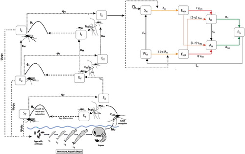
Table 1. Summary of state variables of the model $\left\{\right(1),(2),(3\left)\right\}$.

Variables	Description
E	Number of eggs
$L_j$	Number of larvae at instar stage j (with j=1,2,3,4)
P	Number of pupae
$S_X,E_X,I_X$	Number of susceptible, exposed, and infectious
	female mosquitoes in gonotrophic Stage I, respectively
$S_Y,E_Y,I_Y$	Number of susceptible, exposed, and infectious
	female mosquitoes in gonotrophic Stage II, respectively
$S_Z,E_Z,I_Z$	Number of susceptible, exposed, and infectious,
	female mosquitoes in gonotrophic Stage III, respectively
$S_H$	Number of wholly susceptible humans
$W_H$	Number of susceptible humans with reduced malaria
	susceptibility due to recovery from prior malaria infection
$E_{HN}$	Number of exposed (newly-infected but not infectious) humans without malaria immunity due to prior infection
	(i.e., exposed and malaria-naive humans)
$E_{HR}$	Number of exposed humans with prior partial immunity to malaria
	due to recovery from prior malaria infection
$I_H$	Number of symptomatic infectious humans
$A_H$	Number of asymptomatic infectious humans
$R_H$	Number of recovered humans

Table 2. Description of parameters of the model $\left\{\right(1),(2),(3\left)\right\}$.

Parameters	Description
${\mathrm{\Pi }}_H$	Recruitment rate of humans
${\mu }_H$	Natural death rate of humans
${\rho }_H$	Rate of complete loss of partial immunity (from $W_H$ to $S_H$ class)
$b_H$	Per capita mosquito biting rate in Stage I of the gonotrophic cycle
${\beta }_H$	Transmission probability from infectious mosquitoes to susceptible humans
${\xi }_H$	Rate of loss of infection-acquired immunity (from the $R_H$ to the $W_H$ class)
ε	Modification parameter for the reduction of human susceptibility to malaria infection after recovery from prior malaria infection
${\gamma }_{HN}$	Progression rate of exposed humans without prior malaria immunity to the infectious class (A_H or I_H)
${\gamma }_{HR}$	Progression rate of exposed humans with prior malaria immunity to infectious class
r	Probability of exposed humans without prior malaria immunity showing clinical symptoms of the disease
q	Probability of exposed humans with prior malaria immunity showing clinical symptoms of the disease
${\nu }_H$	Transition rate of symptomatic humans to the asymptomatically-infectious class ($A_H$)
${\delta }_H,{\delta }_{HA}$	Malaria-induced death rates of humans in the infectious class $I_H$ and $A_H$, respectively
${\alpha }_H$	Recovery rate of symptomatically infectious humans
${\alpha }_{HA}$	Recovery rate of asymptomatically infectious humans
${\psi }_E$	Number of eggs laid per oviposition
${\sigma }_E,{\sigma }_P$	Maturation rate of eggs and pupae, respectively
${\sigma }_{Lj}$	Maturation rate of larvae from larval Stage j to Stage j+1 (or to pupa) (for j=1,2,3,4)
f	Proportion of adult mosquitoes that are females
${\mu }_E,{\mu }_L,{\mu }_P,{\mu }_M$	Temperature-dependent death rates of eggs, larvae, pupae and adult mosquitoes, respectively
${\eta }_E,{\eta }_L,{\eta }_P,{\eta }_M$	Temperature-independent death rates for eggs, larvae, pupae and adult female mosquitoes, respectively
$k_L$	Density-dependent mortality rate of larvae
${\beta }_V$	Transmission probability from infectious humans to susceptible mosquitoes
${\theta }_Y$	Rate of progression from Stage II to Stage III of the gonotrophic cycle
${\varphi }_Z$	Rate of oviposition for adult mosquitoes in Stage III of the gonotrophic cycle
${\kappa }_M$	Progression rate of exposed adult female mosquitoes to infectious stage
$K_E$	Carrying capacity of eggs

Table 3. Ranges and baseline values for the temperature-independent parameters of the model (detailed derivation of the values of these parameters is given in Section 2.5).

Parameters	Range	Baseline	Reference
${\mu }_H$	$1/(50\times 365)-1/(70\times 365)$ day^−1	$1/(60\times 365)$ day^−1	See text
${\mathrm{\Pi }}_H$	4−5.5 humans day^−1	4.5 humans day^−1	See text
${\xi }_H$	0.02−−0.0714 day^−1	1/14 day^−1	[82]
${\alpha }_H$	$1/1500-1$ day^−1	1/30 day^−1	[7,89]
${\alpha }_{HA}$	$1/1500-1/100$ day^−1	1/180 day^−1	[7,89]
r, q	0.67−1.0, 0.01−0.33	0.9, 0.33	[23], See text
${\gamma }_{HN}$, ${\gamma }_{HR}$	1/17–1/14 day^−1	1/14 day^−1	[6]
${\delta }_H$	See text	0.0021	[5,28,80], See text
${\delta }_{HA}$	See text	$5.61\times {10}^{-6}$	[5,28,80], See text
$b_H$	0.5−4 day^−1	2 day^−1	[25]
${\beta }_H$	0.01−0.50	0.50	[81,89]
${\nu }_H$	0.001−0.05	1/30	Assumed
ε	0.1−1.0	0.5	[90]
${\beta }_V$	0.02−0.25	0.15	[20,50]
${\rho }_H$	$1/(3\times 365)-1/(7\times 365)$ day^−1	$1/(3\times 365)$ day^−1	[34]
f	0.5−0.8	0.5	[41,63]
${\sigma }_E$	0.33−1 day^−1	0.5	[103]
${\sigma }_P$	0.33−1 day^−1	0.5	[10]
${\eta }_E$	0−0.075 day^−1	0	[87], See text
${\eta }_L$	0−0.6 day^−1	0	[87]
${\eta }_P$	0−0.3 day^−1	0	[87]
${\eta }_M$	0−0.2 day^−1	0	[59,71]
${\varphi }_Z$	0.5−4 day^−1	2 day^−1	[25]
${\psi }_E$	10−150 eggs oviposition^−1	65 eggs oviposition^−1	[92]
$K_E$	$1.0\times {10}^4-1.0\times {10}^6$	$1.0\times {10}^5$	Derived, see text
$k_L$	0−0.0001 larvae^−1 day^−1	0	[2]

The non-autonomous model $\left\{\right(1),(2),(3\left)\right\}$ is an extension of the autonomous model by Ngonghala et al. [66] by, inter alia,

1. Adding the dynamics of immature mosquitoes (i.e., including compartments for eggs, four larval instars and pupae).

2. Adding effect of temperature variability.

3. Adding a compartment (W) for humans with partial immunity due to recovery from prior malaria infection.

4. Allowing for disease transmission by asymptomatically-infectious humans.

5. Stratifying the population of exposed humans in terms of whether they have had prior malaria infection (i.e., splitting the population of malaria-exposed humans into the compartments $E_{HN}$ and $E_{HR}$).

2.5. Estimation of temperature-independent parameters

In this section, the justification for the estimate of the numerical value of each of the temperature-independent parameters of the model $\left\{\right(1),(2),(3\left)\right\}$ is briefly discussed.

2.5.1. Human parameters

We may reasonably estimate ${\rho }_H$, the rate at which malaria-experienced humans revert to a naive state, from the previous work of Filipe et al. [34], who proposed that clinical immunity decays with a half-life of approximately 5 years. If we take 5 years as the expected duration of immunity, then ${\rho }_H=1/(5\times 365)$ day⁻¹. The probability of developing a blood-stage infection after an infectious mosquito bite, ${\beta }_H$ in our model, may range from 0.01 to 0.5. In 1956, Macdonald [53] concluded that only 1 in 20 or 100 (depending upon region) bites containing sporozoites resulted in an actual infection. Similarly, Pull and Grab [78] estimated ${\beta }_H$ at $1.5-2.6\mathrm{\%}$ in Eastern Africa, in 1974, but some more recent works suggest 0.5 as a reasonable value for malaria-naive hosts [81,89]. Also complicating matters, ${\beta }_H$ may be highly variable between individuals [89], and likely decreases somewhat with exposure history, although the effect of prior exposures is likely small [90]. Therefore, a reasonable range for ε, the parameter that accounts for the reduced probability of acquiring infection from an infectious bite for individuals with prior malaria exposure in comparison to malaria-naive individuals, may be 0.1−1.

The delay from initial infection to clinical disease is on the order of about two weeks, as Plasmodium sporozoites first infect hepatocytes, undergoing pre-erythrocyte schizogony, and then there is a “pre-patent” period prior to the first appearance of malaria trophozoites in the blood. For P. falciparum, these stages respectively last 5–7 days and 9–10 days [6], giving ${\gamma }_{HN}$ = ${\gamma }_{HR}$ = 1/17–1/14 day⁻¹. Untreated P. falciparum infections are quite long-lasting, with a variety of classical works concluding that infection could persist for over two years, with parasitemia lasting perhaps 6–10 months on average [7]. For example, Jeffery and Eyles [42] reported a mean infection time of $279.5\pm 19.9$ days, with a range of 114 to 503 days, across 23 inadequately treated malaria patients. As reported by Sama et al. [86], intentional malaria infection was previously used therapeutically against syphilis, with such infections tending to last 200−300 days.

More recently, Sama et al. [86] used a simple mathematical model to re-analyze several datasets and determined average infection times between 602 and 1,329 days, the latter number their estimate for infections in the Garki Project, while another modelling work by Smith et al. [89] concluded that infection might reasonably last 5.5 to 11 months, on average. Case studies of accidental P. falciparum infection leading to asymptomatic infection demonstrate that such parasitemias can last as long as 13 years [7], with a median duration of roughly two years. In sum then, the natural recovery rate for asymptomatic and untreated symptomatic infections may plausibly range from about 1/1500 to 1/100 day⁻¹. Effective treatment rapidly clears blood-stage infections. Thus, the recovery rate for symptomatic humans could be as high as about 1 day⁻¹, if all such patients receive prompt and effective therapy.

The transition rate, ${\xi }_H$, out of the recovered class in which humans are refractory to further infection, is likely rather rapid. This is owing to the fact that Rodriguez-Barraquer et al. [82] observed a median time to re-infection, following treatment, of just 44 days in children in a holoendemic area of Uganda. Drug treatment can confer transient protection against new infections for perhaps a few weeks. Based on these observations, and the fact that new malaria infections have been clinically defined as new febrile episodes with parasitemia occurring at least 14 days after prior infection [82], we assume that mean waiting time in the recovered class is at least 14 days, and no more than 50 days, yielding ${\xi }_H=0.02-0.0714$ day⁻¹. We note that in a modelling work, O'Meara et al. [72] assumed either a 28 or 370 day-long period during which non-immune and semi-immune individuals, respectively, are refractory to reinfection following recovery from malaria, although, due to differences in model formulation, this was not directly comparable to our ${\xi }_H$ parameter.

The excess mortality rate from malaria infection, for malaria-naive patients, can be inferred from case-mortality rates. Considering symptomatic patients, for a given case-fatality fraction denoted ${\tau }_H$, recovery rate ${\alpha }_H$, background mortality rate ${\mu }_H$, and excess mortality rate ${\delta }_H$, we have that the portion of infected humans who die from malaria is (4) ${\tau }_H=\frac{{\delta }_H}{{\alpha }_H+{\mu }_H+{\delta }_H},$(4) and solving for ${\delta }_H$ gives (5) ${\delta }_H=\frac{{\tau }_H({\alpha }_H+{\mu }_H)}{1-{\tau }_H}.$(5) Similar relations hold for asymptomatic patients and ${\tau }_{HA}$, ${\alpha }_{HA}$, and ${\delta }_{HA}$.

For previously unexposed patients, case-mortality is on the order of at least $1-2\mathrm{\%}$, even when there is access to treatment, and is more generally in the $5-20\mathrm{\%}$ range [5]. Despite treatment, case-fatality rates are quite high in children suffering from severe disease, who have limited (if any) immunity, and was 8.5% in one trial of sub-Saharan children receiving highly effective artesunate [28]. In a large study conducted in Northeastern Tanzania [80], 0.9% of 5,076 parasite-positive patients presenting to hospital and deemed to have non-severe disease died, while 7% of 1,984 patients with severe disease succumbed. We can conclude that average excess mortality from a single episode of symptomatic mortality is probably in the 1–20% range (with $3-5\mathrm{\%}$ a reasonable default estimate), while asymptomatic malaria kills (directly or indirectly) <1% of sufferers.

Since the majority of symptomatic patients do not suffer severe malaria, and by adolescence most malaria presents as uncomplicated febrile disease, if at all [23], we assume, in our model framework, that the majority of malaria-experience patients who are re-infected are unlikely to develop severe disease. In particular, we set $q\le 0.33$. On the other hand, given how deadly malaria is in those with no prior experience of it, it is likely that very few of these patients are initially asymptomatic. Hence, we set $r\ge 0.67$.

Human birth and natural death rates are assumed to occur according to first-order kinetics at rates ${\mathrm{\Pi }}_H$ and ${\mu }_H$, respectively. This implies an exponential age distribution for the population, which is generally unrealistic (as the probability of death increases with age). Nevertheless, if we suppose an average lifespan of Φ days and a steady-state population of Ω (in the absence of malaria-induced mortality), then ${\mu }_H$ follows easily as $1/\mathrm{\Phi }$, and ${\mathrm{\Pi }}_H={\mu }_H\mathrm{\Omega }$. We might reasonably assume Φ in the 50−70 year range, and while Ω is location-specific, supposing Ω = ${10}^5$ individuals (which is the typical size of towns/communities in endemic areas in sub-Saharan Africa), then ${\mathrm{\Pi }}_H\approx$ 4–5.5 persons day⁻¹. It should also be noted that in the well-mixed setting, Ω are ${\mathrm{\Pi }}_H$ are essentially arbitrary.

2.5.2. Mosquito parameters

Roughly half (42−63%) of An. stephensi mosquitoes fed gametocyte-rich cultures in a laboratory setting went on to develop detectable sporozoites [81], implying ${\beta }_V$ of about 0.5. However, field studies suggest lower values: One study [50] of five villages in a holoendemic area of Northern Tanzania finding ${\beta }_V$ to be 21% for An. gambiae, while Charlwood et al. [20] estimated the same parameter to be either 1.9% for An. gambiae or 3.4% for An. funestus in southern Tanzania, and as reviewed in [38,50], most previous estimates in Africa have been on the order of 5−15%. It should further be noted that a genuine increase in infectivity of humans to mosquitoes (in Africa) may have occurred between earlier work in the 1960s and the 1990s, likely due to widespread chloroquine use in the earlier era that suppressed transmission, and possibly exerted selective pressure for increased virulence [50]. Overall, 0.02−0.25 seems a reasonable range for ${\beta }_V$ in the field.

The number of eggs per oviposition event, ${\psi }_E$, may vary from 10 to 150 for An. gambiae [3,92], but is typically about 40 to 85 under field conditions [3]. In a laboratory setting, the female fraction of emerging imago, f, was about 0.5 under nutrient replete conditions but almost 0.8 with larval competition for food [41], and a field study [63] showed a slight female preference (f=0.57) among emerging An. gambiae s.l.. Eggs hatch into larvae in 1−3 days, and while this is a temperature-dependent process, most eggs hatch by the third day regardless [103], and therefore as a first approximation the maturation rate for eggs, ${\sigma }_E$, is assumed constant and in the range 0.33−1 day⁻¹. Similarly, pupae hatch within a few days [10], and we therefore take ${\sigma }_P=0.33-1$ day⁻¹, with all temperature-dependence manifested at the larval stage of development.

The Anopheles egg carrying capacity, $K_E$, and density-dependent larval competition coefficient, $k_L$, are lumped measures of the habitat and resources available for mosquito breeding, and are therefore expected to be highly variable. If $k_L=0$, and if we suppose that the mosquitoes per human ratio, M, is anywhere from 0.01 to 100 mosquitoes person⁻¹, then we can get a very crude idea of the magnitude of $K_E$ by assuming an average larval development time, d, of 15 days, and average daily survival probability, p=0.8, and an expected adult survival time, s, of perhaps 10 days, and therefore giving (6) $K_E=\frac{M\mathrm{\Omega }}{s{p}^d}\approx 3M\mathrm{\Omega }\approx 0.03\mathrm{\Omega }-300\mathrm{\Omega }.$(6)

We estimate temperature-independent death rates for larvae and pupae, ${\eta }_L$, and ${\eta }_P$, respectively, from life table analysis of An. gambiae larvae and pupae sampled from either a marsh or burrow-pits in Kenya [87]. This study suggested a net larval death rate ${\eta }_L+{\mu }_L$ ranging 0.07115–0.33273 day⁻¹ (mean 0.2064) and 0.06373–0.588251 day⁻¹(mean 0.3154) for the marsh and burrow-pits, respectively, while respective pupal death rates, ${\eta }_P+{\mu }_P$, were 0.18350 and 0.32577 day⁻¹. Since ${\mu }_L,{\mu }_P\ge 0$, we suppose these are upper limits to ${\eta }_L$. Moreover, we assume that eggs have a total death rate similar to first larval instars, which was 0.06373 or 0.07115 in [87], suggesting ${\eta }_E$ is small. Field studies [59,71] suggest adult mosquito daily survival probabilities typically in the 0.80 to 0.95 range, for An. gambiae and An. funestus, and thus we may reasonably assume ${\eta }_M+{\mu }_M$ on the order of 0.05–0.25 day⁻¹, or perhaps 0–0.2 day⁻¹ for ${\eta }_M$.

Temperature-independent parameter values and ranges are summarized in Table 3.

2.6. Functional forms of thermal-response functions

The functional forms of the thermal response (temperature-dependent) functions in the model are formulated based on available laboratory data and prior work as follows. The mean death rates, ${\mu }_M\left(T_A\right)$, for adult Anopheles, are determined using data from [9], who reported An. gambiae survival in a laboratory setting under constant ambient temperatures ranging from 5 to 40${}^{\circ }$C (in 5${}^{\circ }$C intervals), and for a range of relative humidities. We use the survival curve for $60\mathrm{\%}$ relative humidity, and fit a quadratic polynomial as follows: $\frac{1}{{\mu }_M\left(T_A\right)}=max(-11.8239+3.3292T_A-0.0771T_A^2,0.1).$ Using larval survival times reported by Bayoh and Lindsay [11], we fit the per-capita death rate (inverse of survival time) of the immature mosquitoes (${\mu }_E,{\mu }_L,$ and ${\mu }_P$) fairly well using the following fourth-order polynomial (for i=E,L,P): ${\mu }_i\left(T_W\right)=8.929\times {10}^{-6}{T}_W^4-9.271\times {10}^{-4}{T}_W^3+3.536\times {10}^{-2}{T}_W^2-0.5814T_W+\mathrm{3.509.}$ Eggs hatch into larvae in 1−3 days, and while this is a temperature-dependent process, most eggs hatch by the third day regardless [103], and therefore as a first approximation the maturation rate for eggs, ${\sigma }_E$, is assumed constant and in the range 0.33−1 day⁻¹. Similarly, pupae hatch within a few days [10], and thus we assume ${\sigma }_P$ = 0.33−1 day⁻¹. Moreover, larval development is described using the unimodal relation derived by Bayoh and Lindsay [10], where the overall time from egg to adult, denoted by ${\mathcal{D}}_{EA}\left(T_W\right)$, is described as (7) ${\mathcal{D}}_{EA}\left(T_W\right)=(a+b{T}_W+c{e}^{T_W}+d{e}^{-T_W}{)}^{-1},$(7) with a=−0.05, b=0.005, $c=-2.139\times {10}^{-16}$, and $d=-2.81357\times {10}^5$. We assume that all four larval stages are equal in duration, from which it follows that ${\sigma }_{L_j}\left(T_W\right)=4{\left({\mathcal{D}}_{EA}\left(T_W\right)-\frac{1}{{\sigma }_E}-\frac{1}{{\sigma }_P}\right)}^{-1}\mathrm{for}j=1,2,3,4.$ Note, finally, that we restrict ${\sigma }_{L_j}\left(T_W\right)$ to be strictly positive.

The transition rate from exposed mosquito class to infectious mosquito (${\kappa }_M\left(T_A\right)$) is the inverse of the mean sporogonic cycle duration (in days). We describe the duration of sporogony using the formula of Moshkovsky [25,67], but with the further restrictions that sporogony cannot progress either below 16 ${}^{\circ }$C or above 40 ${}^{\circ }$C, giving ${\kappa }_M\left(T_A\right)=\left\{\begin{array}{ll}\frac{T_A-T_{min}}{D},& \mathrm{if}{16}^{\circ }\mathrm{C}<T_A<{40}^{\circ }\mathrm{C},\\ 0,& \mathrm{if}{T}_A\le {16}^{\circ }\mathrm{C},T_A\ge {40}^{\circ }\mathrm{C}.\end{array}\right.$ where D=111 and $T_{min}={16}^{\circ }$C [25].

Similarly, the rate at which mosquitoes complete Stage II of the gonotrophic cycle (i.e., the transition rate from the Y to Z compartments) is described using Moshkovky's formula [25,67]: ${\theta }_Y\left(T_A\right)=\left\{\begin{array}{ll}\frac{T_A-9.9}{36.5},& \mathrm{if}{9.9}^{\circ }\mathrm{C}<T_A<{40}^{\circ }\mathrm{C},\\ 0,& \mathrm{if}{T}_A\le {9.9}^{\circ }\mathrm{C},T_A\ge {40}^{\circ }\mathrm{C}.\end{array}\right.$Furthermore, as a first approximation, we assume air and water temperature to be equal for all t (i.e., $T_A\left(t\right)=T_W\left(t\right)$), although some studies have used a linear offset between air and water temperature [4], and air and water temperatures are expected to be dissimilar in general, with the relationship changing over the course of the day [74]. In some of our theoretical analysis (particularly in Section 3), we assume that ambient temperature is constant. However, in some other settings (particularly in some of our numerical simulations, such as in Section 4.1.1), we assume daily fluctuations in ambient temperature. When such daily fluctuations are considered, we employ the following sinusoidal function to capture hourly changes in the ambient temperature: (8) $T_A\left(t\right)=T_{A0}-\frac{\mathrm{DTR}}{2}\sin [\frac{2\pi }{24}(t_h+14)],$(8) where $T_{A0}$ is the mean daily air temperature, the daily temperature range (DTR) is the magnitude of variation about the mean (twice the amplitude of the sinusoid), and $t_h\in [0,24)$ is the time in hours for any given day. The profiles of some of the temperature-dependent parameters of the model are depicted in Figure 3.

Figure 3. Profile of temperature-dependent parameters of the model $\{$(1(1) $\begin{array}{rl}\frac{\mathrm{d}E}{\mathrm{d}t}& ={\psi }_E{\varphi }_Z{\left(1-\frac{E}{K_E}\right)}_{+}(S_Z+E_Z+I_Z)-[{\sigma }_E\left(T_W\right)+{\eta }_E+{\mu }_E]E,\\ \frac{\mathrm{d}{L}_1}{\mathrm{d}t}& ={\sigma }_E\left(T_W\right)E-[{\sigma }_{L_1}\left(T_W\right)+{\eta }_L+k_{L}L+{\mu }_L\left(T_W\right)]L_1,\\ \frac{\mathrm{d}{L}_j}{\mathrm{d}t}& ={\sigma }_{L_{(j-1)}}\left(T_W\right)L_{j-1}-[{\sigma }_{Lj}\left(T_W\right)+{\eta }_L+k_{L}L+{\mu }_L\left(T_W\right)]L_j,j=2,3,4,\\ \frac{\mathrm{d}P}{\mathrm{d}t}& ={\sigma }_{L_4}\left(T_W\right)L_4-[{\sigma }_P\left(T_W\right)+{\eta }_P+{\mu }_P]P.\end{array}$(1) )–(3(3) $\begin{array}{rl}\frac{\mathrm{d}{S}_H}{\mathrm{d}t}& ={\mathrm{\Pi }}_H-{\lambda }_H{S}_H+{\rho }_H{W}_H-{\mu }_H{S}_H,\\ \frac{\mathrm{d}{W}_H}{\mathrm{d}t}& ={\xi }_H{R}_H-(1-ϵ){\lambda }_H{W}_H-({\rho }_H+{\mu }_H)W_H,\\ \frac{\mathrm{d}{E}_{HN}}{\mathrm{d}t}& ={\lambda }_H{S}_H-({\gamma }_{HN}+{\mu }_H)E_{HN},\\ \frac{\mathrm{d}{E}_{HR}}{\mathrm{d}t}& =(1-ϵ){\lambda }_H{W}_H-({\gamma }_{HR}+{\mu }_H)E_{HR},\\ \frac{\mathrm{d}{I}_H}{\mathrm{d}t}& =r{\gamma }_{HN}{E}_{HN}+q{\gamma }_{HR}{E}_{HR}-({\alpha }_H+{\nu }_H+{\mu }_H+{\delta }_H)I_H,\\ \frac{\mathrm{d}{A}_H}{\mathrm{d}t}& =(1-r){\gamma }_{HN}{E}_{HN}+(1-q){\gamma }_{HR}{E}_{HR}+{\nu }_H{I}_H-({\alpha }_{HA}+{\mu }_H+{\delta }_{HA})A_H,\\ \frac{\mathrm{d}{R}_H}{\mathrm{d}t}& ={\alpha }_H{I}_H+{\alpha }_{HA}{A}_H-({\xi }_H+{\mu }_H)R_H,\end{array}$(3) )$\}$: (a) Survival time of larvae, $\left({\mu }_L\right(T_W){)}^{-1}$ (b) Survival time of adult mosquitoes, $\left({\mu }_M\right(T_W){)}^{-1}$ (c) Sporogonic cycle duration in adult female mosquitoes, $\left({\kappa }_M\right(T_A){)}^{-1}$ (d) Duration of Stage II of the gonotrophic cycle, $\left({\theta }_Y\right(T_A){)}^{-1}$, and (e) total time for immature mosquito development.

2.7. Basic qualitative properties

In this section, the basic qualitative properties of the developed model,given by the equations $\{$(1(1) $\begin{array}{rl}\frac{\mathrm{d}E}{\mathrm{d}t}& ={\psi }_E{\varphi }_Z{\left(1-\frac{E}{K_E}\right)}_{+}(S_Z+E_Z+I_Z)-[{\sigma }_E\left(T_W\right)+{\eta }_E+{\mu }_E]E,\\ \frac{\mathrm{d}{L}_1}{\mathrm{d}t}& ={\sigma }_E\left(T_W\right)E-[{\sigma }_{L_1}\left(T_W\right)+{\eta }_L+k_{L}L+{\mu }_L\left(T_W\right)]L_1,\\ \frac{\mathrm{d}{L}_j}{\mathrm{d}t}& ={\sigma }_{L_{(j-1)}}\left(T_W\right)L_{j-1}-[{\sigma }_{Lj}\left(T_W\right)+{\eta }_L+k_{L}L+{\mu }_L\left(T_W\right)]L_j,j=2,3,4,\\ \frac{\mathrm{d}P}{\mathrm{d}t}& ={\sigma }_{L_4}\left(T_W\right)L_4-[{\sigma }_P\left(T_W\right)+{\eta }_P+{\mu }_P]P.\end{array}$(1) )–(3(3) $\begin{array}{rl}\frac{\mathrm{d}{S}_H}{\mathrm{d}t}& ={\mathrm{\Pi }}_H-{\lambda }_H{S}_H+{\rho }_H{W}_H-{\mu }_H{S}_H,\\ \frac{\mathrm{d}{W}_H}{\mathrm{d}t}& ={\xi }_H{R}_H-(1-ϵ){\lambda }_H{W}_H-({\rho }_H+{\mu }_H)W_H,\\ \frac{\mathrm{d}{E}_{HN}}{\mathrm{d}t}& ={\lambda }_H{S}_H-({\gamma }_{HN}+{\mu }_H)E_{HN},\\ \frac{\mathrm{d}{E}_{HR}}{\mathrm{d}t}& =(1-ϵ){\lambda }_H{W}_H-({\gamma }_{HR}+{\mu }_H)E_{HR},\\ \frac{\mathrm{d}{I}_H}{\mathrm{d}t}& =r{\gamma }_{HN}{E}_{HN}+q{\gamma }_{HR}{E}_{HR}-({\alpha }_H+{\nu }_H+{\mu }_H+{\delta }_H)I_H,\\ \frac{\mathrm{d}{A}_H}{\mathrm{d}t}& =(1-r){\gamma }_{HN}{E}_{HN}+(1-q){\gamma }_{HR}{E}_{HR}+{\nu }_H{I}_H-({\alpha }_{HA}+{\mu }_H+{\delta }_{HA})A_H,\\ \frac{\mathrm{d}{R}_H}{\mathrm{d}t}& ={\alpha }_H{I}_H+{\alpha }_{HA}{A}_H-({\xi }_H+{\mu }_H)R_H,\end{array}$(3) )$\}$, will be explored.

Lemma 2.1

Each component of the solution of the model $\{$(1(1) $\begin{array}{rl}\frac{\mathrm{d}E}{\mathrm{d}t}& ={\psi }_E{\varphi }_Z{\left(1-\frac{E}{K_E}\right)}_{+}(S_Z+E_Z+I_Z)-[{\sigma }_E\left(T_W\right)+{\eta }_E+{\mu }_E]E,\\ \frac{\mathrm{d}{L}_1}{\mathrm{d}t}& ={\sigma }_E\left(T_W\right)E-[{\sigma }_{L_1}\left(T_W\right)+{\eta }_L+k_{L}L+{\mu }_L\left(T_W\right)]L_1,\\ \frac{\mathrm{d}{L}_j}{\mathrm{d}t}& ={\sigma }_{L_{(j-1)}}\left(T_W\right)L_{j-1}-[{\sigma }_{Lj}\left(T_W\right)+{\eta }_L+k_{L}L+{\mu }_L\left(T_W\right)]L_j,j=2,3,4,\\ \frac{\mathrm{d}P}{\mathrm{d}t}& ={\sigma }_{L_4}\left(T_W\right)L_4-[{\sigma }_P\left(T_W\right)+{\eta }_P+{\mu }_P]P.\end{array}$(1) )–(3(3) $\begin{array}{rl}\frac{\mathrm{d}{S}_H}{\mathrm{d}t}& ={\mathrm{\Pi }}_H-{\lambda }_H{S}_H+{\rho }_H{W}_H-{\mu }_H{S}_H,\\ \frac{\mathrm{d}{W}_H}{\mathrm{d}t}& ={\xi }_H{R}_H-(1-ϵ){\lambda }_H{W}_H-({\rho }_H+{\mu }_H)W_H,\\ \frac{\mathrm{d}{E}_{HN}}{\mathrm{d}t}& ={\lambda }_H{S}_H-({\gamma }_{HN}+{\mu }_H)E_{HN},\\ \frac{\mathrm{d}{E}_{HR}}{\mathrm{d}t}& =(1-ϵ){\lambda }_H{W}_H-({\gamma }_{HR}+{\mu }_H)E_{HR},\\ \frac{\mathrm{d}{I}_H}{\mathrm{d}t}& =r{\gamma }_{HN}{E}_{HN}+q{\gamma }_{HR}{E}_{HR}-({\alpha }_H+{\nu }_H+{\mu }_H+{\delta }_H)I_H,\\ \frac{\mathrm{d}{A}_H}{\mathrm{d}t}& =(1-r){\gamma }_{HN}{E}_{HN}+(1-q){\gamma }_{HR}{E}_{HR}+{\nu }_H{I}_H-({\alpha }_{HA}+{\mu }_H+{\delta }_{HA})A_H,\\ \frac{\mathrm{d}{R}_H}{\mathrm{d}t}& ={\alpha }_H{I}_H+{\alpha }_{HA}{A}_H-({\xi }_H+{\mu }_H)R_H,\end{array}$(3) )$\}$, subject to non-negative initial conditions, remains nonnegative and bounded for all t>0.

The proof of Lemma 2.1 is given in Appendix 1. Furthermore, consider the following feasible region for the model $\{$(1(1) $\begin{array}{rl}\frac{\mathrm{d}E}{\mathrm{d}t}& ={\psi }_E{\varphi }_Z{\left(1-\frac{E}{K_E}\right)}_{+}(S_Z+E_Z+I_Z)-[{\sigma }_E\left(T_W\right)+{\eta }_E+{\mu }_E]E,\\ \frac{\mathrm{d}{L}_1}{\mathrm{d}t}& ={\sigma }_E\left(T_W\right)E-[{\sigma }_{L_1}\left(T_W\right)+{\eta }_L+k_{L}L+{\mu }_L\left(T_W\right)]L_1,\\ \frac{\mathrm{d}{L}_j}{\mathrm{d}t}& ={\sigma }_{L_{(j-1)}}\left(T_W\right)L_{j-1}-[{\sigma }_{Lj}\left(T_W\right)+{\eta }_L+k_{L}L+{\mu }_L\left(T_W\right)]L_j,j=2,3,4,\\ \frac{\mathrm{d}P}{\mathrm{d}t}& ={\sigma }_{L_4}\left(T_W\right)L_4-[{\sigma }_P\left(T_W\right)+{\eta }_P+{\mu }_P]P.\end{array}$(1) )–(3(3) $\begin{array}{rl}\frac{\mathrm{d}{S}_H}{\mathrm{d}t}& ={\mathrm{\Pi }}_H-{\lambda }_H{S}_H+{\rho }_H{W}_H-{\mu }_H{S}_H,\\ \frac{\mathrm{d}{W}_H}{\mathrm{d}t}& ={\xi }_H{R}_H-(1-ϵ){\lambda }_H{W}_H-({\rho }_H+{\mu }_H)W_H,\\ \frac{\mathrm{d}{E}_{HN}}{\mathrm{d}t}& ={\lambda }_H{S}_H-({\gamma }_{HN}+{\mu }_H)E_{HN},\\ \frac{\mathrm{d}{E}_{HR}}{\mathrm{d}t}& =(1-ϵ){\lambda }_H{W}_H-({\gamma }_{HR}+{\mu }_H)E_{HR},\\ \frac{\mathrm{d}{I}_H}{\mathrm{d}t}& =r{\gamma }_{HN}{E}_{HN}+q{\gamma }_{HR}{E}_{HR}-({\alpha }_H+{\nu }_H+{\mu }_H+{\delta }_H)I_H,\\ \frac{\mathrm{d}{A}_H}{\mathrm{d}t}& =(1-r){\gamma }_{HN}{E}_{HN}+(1-q){\gamma }_{HR}{E}_{HR}+{\nu }_H{I}_H-({\alpha }_{HA}+{\mu }_H+{\delta }_{HA})A_H,\\ \frac{\mathrm{d}{R}_H}{\mathrm{d}t}& ={\alpha }_H{I}_H+{\alpha }_{HA}{A}_H-({\xi }_H+{\mu }_H)R_H,\end{array}$(3) )$\}$: $\begin{array}{rl}\mathrm{\Omega }& =\{\mathcal{B}\left(t\right)\in {\mathbb{R}}_{+}^{22}:N_H\left(t\right)\le \frac{{\mathrm{\Pi }}_H}{{\mu }_H},0\le E\left(t\right)<K_E,0\le L_j\left(t\right)\le {\overline{L}}_j(j=1,2,3,4),\\ & 0\le P\left(t\right)\le \overline{P},0\le N_V\left(t\right)\le {\overline{N}}_V\},\end{array}$ where, $\mathcal{B}=(S_H,W_H,E_{HN},E_{HR},I_H,A_H,R_H,E,L_1,L_2,L_3,L_4,P,S_X,E_X,I_X,S_Y,E_Y,I_Y,S_Z,E_Z,I_Z),$ and, ${\overline{L}}_j(j=1,2,3,4),\overline{P}$, ${\overline{N}}_V$ are defined in Appendix 1. It follows from Lemma 2.1 that Ω is positively-invariant for the model $\left\{\right(1),(2),(3\left)\right\}$. Therefore, it is sufficient to consider the dynamics of the model in Ω [40].

3. Analysis of autonomous version of the model

It is instructive, first of all, to gain insight into the dynamics of the autonomous version of the model $\left\{\right(1),(2),(3\left)\right\}$. That is, we are studying the dynamics of the model for the case where all temperature-dependent parameters of the model are considered to be constants (i.e., we consider the model $\left\{\right(1),(2),(3\left)\right\}$ with ${\mu }_M\left(T_A\right)={\mu }_M,{\mu }_i\left(T_W\right)={\mu }_i(i=E,L,P),{\sigma }_{L_j}\left(T_W\right)={\sigma }_{L_j}(j=1,2,3,4),{\kappa }_M\left(T_A\right)={\kappa }_M$ and ${\theta }_Y\left(T_A\right)={\theta }_Y$). The model $\left\{\right(1),(2),(3\left)\right\}$ with the temperature-dependent parameters treated as constant is denoted as the autonomous model. It is convenient to define the threshold quantity ${\mathcal{R}}_{MP}=\frac{{\psi }_E{\varphi }_Z{\sigma }_E{\displaystyle \prod _{k=1}^4{\sigma }_{Lk}f{\sigma }_P{\theta }_Y{b}_H}}{({\sigma }_E+{\eta }_E+{\mu }_E)({\sigma }_P+{\eta }_P+{\mu }_P)(C_X{C}_Y{C}_Z-{\theta }_Y{b}_H{\varphi }_Z){\displaystyle \prod _{k=1}^4({\sigma }_{Lk}+{\eta }_L+{\mu }_L)}},$ where $C_X=b_H+{\eta }_M+{\mu }_M$, $C_Y={\theta }_Y+{\eta }_M+{\mu }_M$, $C_Z={\varphi }_Z+{\eta }_M+{\mu }_M$ and $C_X{C}_Y{C}_Z-{\theta }_Y{b}_H{\varphi }_Z=({\eta }_M+{\mu }_M)\left[C_Z\right(C_X+{\theta }_Y)+b_H{\theta }_Y]>0$ (so that ${\mathcal{R}}_{MP}>0$).

The threshold quantity (${\mathcal{R}}_{MP}$) is similar to the vectorial reproduction number described in [70], for which mosquito population exists whenever ${\mathcal{R}}_{MP}>1$ (and no mosquito exists for ${\mathcal{R}}_{MP}\le 1$). Ecologically, ${\mathcal{R}}_{MP}$ measures the average number of new adult female mosquitoes produced by one reproductive mosquito during its entire reproductive period.

3.1. Existence and asymptotic stability of disease-free equilibria

The autonomous model has:

1. a trivial disease-free equilibrium (where no mosquitoes exist), given by: ${\mathcal{T}}_0=\left(\frac{{\mathrm{\Pi }}_H}{{\mu }_H},0,0,0,0,0,0,0,0,0,0,0,0,0,0,0,0,0,0,0,0,0\right).$

2. at least one non-trivial disease-free equilibrium (NDFE) if and only if ${\mathcal{R}}_{MP}>1$. The NDFE is unique when the density-dependent larval mortality rate ($k_L$) is set to zero. The unique NDFE is given by ${\mathcal{E}}_0=\left(\frac{{\mathrm{\Pi }}_H}{{\mu }_H},0,0,0,0,0,0,E^{\diamond },L_1^{\diamond },L_2^{\diamond },L_3^{\diamond },L_4^{\diamond },P^{\diamond },S_X^{\diamond },0,0,S_Y^{\diamond },0,0,S_Z^{\diamond },0,0\right),$ where, (9) $\begin{array}{rl}& E_V^{\diamond }=K_E(1-\frac{1}{{\mathcal{R}}_{MP}}),L_1^{\diamond }=\frac{{\sigma }_E}{C_{L1}}{E}^{\diamond },L_j^{\diamond }=\frac{{\sigma }_{L_{j-1}}}{C_{Lj}}{L}_{j-1}^{\diamond },j=2,3,4,\\ & P_V^{\diamond }=\frac{{\sigma }_{L_4}}{C_P}{L}_4^{\diamond },\\ & S_X^{\diamond }=\frac{1}{C_X}(f{\sigma }_P{P}^{\diamond }+{\varphi }_Z{S}_Z^{\diamond }),S_Y^{\diamond }=\frac{1}{C_Y}{b}_H{S}_X^{\diamond },S_Z^{\diamond }=\frac{{\theta }_Y{b}_{H}f{\sigma }_P{P}^{\diamond }}{C_X{C}_Y{C}_Z-{\theta }_Y{b}_H{\varphi }_Z},\end{array}$(9) with $C_{Lj}={\sigma }_{Lj}+{\eta }_L+{\mu }_L(j=1,2,3,4)$, $C_P={\sigma }_P+{\eta }_P+{\mu }_P$.

It should be noted that since mosquitoes always exist in malaria-endemic regions, the asymptotic stability property of the trivial disease-free equilibrium (${\mathcal{T}}_0$) is not analyzed in this study (since ${\mathcal{T}}_0$ is unrealistic ecologically).

NDFE: special case

Consider the special case of the autonomous model with no density-dependent larval mortality (i.e., $k_L=0$). Furthermore, let ${\mathcal{R}}_{MP}>1$ (so that the unique NDFE, ${\mathcal{E}}_0$, exists). It can be shown, using the next generation operator method [27,96], that the associated reproduction number of the autonomous model (denoted by ${\mathcal{R}}_0$) is given by: (10) ${\mathcal{R}}_0=\sqrt{{\mathcal{R}}_{HV}\times {\mathcal{R}}_{VH}},$(10) where, (11) ${\mathcal{R}}_{HV}=b_H{\beta }_V\frac{S_X^{\diamond }}{N_H^{\ast }}[\frac{r{\gamma }_{HN}}{g_1}\frac{1}{g_3}+\frac{r{\gamma }_{HN}}{g_1}\frac{{\nu }_H}{g_3}\frac{1}{g_4}+\frac{(1-r){\gamma }_{HN}}{g_1}\frac{1}{g_4}],$(11) and, (12) ${\mathcal{R}}_{VH}=b_H{\beta }_H\frac{S_H^{\diamond }}{N_H^{\ast }}\frac{{\kappa }_M{\varphi }_Z{\theta }_Y(C_Y{C}_Z+C_Y{g}_X+g_X{g}_Z)}{(C_X{C}_Y{C}_Z-b_H{\varphi }_Z{\theta }_Y)(g_X{g}_Y{g}_Z-b_H{\varphi }_Z{\theta }_Y)},$(12) with $N_H^{\ast }={\mathrm{\Pi }}_H/{\mu }_H$, $g_1={\gamma }_{HN}+{\mu }_H$, $g_2={\gamma }_{HR}+{\mu }_H$, $g_3={\alpha }_H+{\nu }_H+{\delta }_H+{\mu }_H$, $g_4={\alpha }_{HA}+{\delta }_{HA}+{\mu }_H$, $g_X=C_X+{\kappa }_M$, $g_Y=C_Y+{\kappa }_M$, $g_Z=C_Z+{\kappa }_M$. The result below follows from Theorem 2 of [96].

Theorem 3.1

The NDFE, ${\mathcal{E}}_0$, of the autonomous model with $k_L=0$ and ${\mathcal{R}}_{EP}>1$ is locally-asymptotically stable in $\mathrm{\Omega }\setminus \left\{{\mathcal{T}}_0\right\}$ if ${\mathcal{R}}_0<1$, and unstable if ${\mathcal{R}}_0>1$.

Interpretation of ${\mathcal{R}}_0$

The threshold quantity ${\mathcal{R}}_0$, given by Equation (10(10) ${\mathcal{R}}_0=\sqrt{{\mathcal{R}}_{HV}\times {\mathcal{R}}_{VH}},$(10) ), measures the average number of new infections in humans (vectors) generated by an infectious vector (human). Its components are epidemiologically interpreted as follows.

1. Interpretation of ${\mathcal{R}}_{HV}$: The quantity ${\mathcal{R}}_{HV}$, given by (11(11) ${\mathcal{R}}_{HV}=b_H{\beta }_V\frac{S_X^{\diamond }}{N_H^{\ast }}[\frac{r{\gamma }_{HN}}{g_1}\frac{1}{g_3}+\frac{r{\gamma }_{HN}}{g_1}\frac{{\nu }_H}{g_3}\frac{1}{g_4}+\frac{(1-r){\gamma }_{HN}}{g_1}\frac{1}{g_4}],$(11) ), is associated with the infection of susceptible mosquitoes by infectious (asymptomatic and symptomatic) humans. It can further be expressed as (13) ${\mathcal{R}}_{HV}={\mathcal{R}}_{I_{H}V}+{\mathcal{R}}_{A_{H}V},$(13) where, $\begin{array}{rl}& {\mathcal{R}}_{I_{H}V}=b_H{\beta }_V\frac{S_X^{\diamond }}{N_H^{\ast }}\frac{r{\gamma }_{HN}}{g_1}\frac{1}{g_3}\mathrm{and}\\ & {\mathcal{R}}_{A_{H}V}=b_H{\beta }_V\frac{S_X^{\diamond }}{N_H^{\ast }}[\frac{r{\gamma }_{HN}}{g_1}\frac{{\nu }_H}{g_3}+\frac{(1-r){\gamma }_{HN}}{g_1}]\frac{1}{g_4},\end{array}$ with ${\mathcal{R}}_{I_{H}V}$ accounting for the average number of new infectious adult female mosquitoes generated by symptomatically infectious humans ($I_H$) and ${\mathcal{R}}_{A_{H}V}$ measures the average number of new infectious adult female mosquitoes generated by asymptomatically infectious humans ($A_H$).

2. Interpretation of ${\mathcal{R}}_{VH}$: The threshold quantity ${\mathcal{R}}_{VH}$, given by (12(12) ${\mathcal{R}}_{VH}=b_H{\beta }_H\frac{S_H^{\diamond }}{N_H^{\ast }}\frac{{\kappa }_M{\varphi }_Z{\theta }_Y(C_Y{C}_Z+C_Y{g}_X+g_X{g}_Z)}{(C_X{C}_Y{C}_Z-b_H{\varphi }_Z{\theta }_Y)(g_X{g}_Y{g}_Z-b_H{\varphi }_Z{\theta }_Y)},$(12) ), is associated with the infection of susceptible humans by infected mosquitoes at Stage I of the gonotrophic cycle ($I_X$). It can further be expressed as (14) ${\mathcal{R}}_{VH}=b_H{\beta }_H\frac{S_H^{\diamond }}{N_H^{\ast }}\frac{1}{C_X}({\mathcal{R}}_{V1H}+{\mathcal{R}}_{V2H}+{\mathcal{R}}_{V3H}),$(14) where, ${\mathcal{R}}_{V1H},{\mathcal{R}}_{V2H}$ and ${\mathcal{R}}_{V3H}$ account for all possible routes at which an exposed mosquito in Stage II of the gonotrophic cycle ($E_Y$) mosquito survives to become (and remain) an infected mosquito at Stage I of the gonotrophic cycle ($I_X$) (i.e., the sum ${\mathcal{R}}_{V1H}+{\mathcal{R}}_{V2H}+{\mathcal{R}}_{V3H}$ is the probability that an exposed mosquito in $E_Y$ class survives to become an infected mosquito in $I_X$ class). Consider the following definitions:

Definition 3.1

1. $X\to Y$ means the fraction of adult mosquitoes that survives the X class and moves to the Y class;

2. $X\to Y\to Z$ is the product of the proportions of adult mosquitoes that survived $X\to Y$ and $Y\to Z$ transmissions;

3. $(\to X\to Y\to Z{)}^j=\to X\to Y\to Z\to X\to Y\to Z\to \cdots \to X\to Y\to Z$ (j times, $j\in \mathbb{N}$). That is, for j=2, $(\to X\to Y\to Z{)}^2=\to X\to Y\to Z\to X\to Y\to Z$.

4. $(\to X\to Y\to Z{)}^0=1$.

Thus, the quantities ${\mathcal{R}}_{V1H},{\mathcal{R}}_{V2H}$ and ${\mathcal{R}}_{V3H}$ defined in Equation 14(14) ${\mathcal{R}}_{VH}=b_H{\beta }_H\frac{S_H^{\diamond }}{N_H^{\ast }}\frac{1}{C_X}({\mathcal{R}}_{V1H}+{\mathcal{R}}_{V2H}+{\mathcal{R}}_{V3H}),$(14) can be described as follows:

1. The quantity ${\mathcal{R}}_{V1H}$, which accounts for the infection route (for $j,k\in \mathbb{Z}$) $E_Y\to E_Z\to E_X(\to E_Y\to E_Z\to E_X{)}^j\to I_X(\to I_Y\to I_Z\to I_X{)}^k,$ is given by ${\mathcal{R}}_{V1H}=\frac{{\theta }_Y}{g_Y}\frac{{\varphi }_Z}{g_Z}\times \sum _{j=0}^n(\frac{b_H}{g_X}\frac{{\theta }_Y}{g_Y}\frac{{\varphi }_Z}{g_Z}{)}^j\times \frac{{\kappa }_M}{g_X}\times \sum _{k=0}^m(\frac{b_H}{C_X}\frac{{\theta }_Y}{C_Y}\frac{{\varphi }_Z}{C_Z}{)}^k.$ That is, there are two routes for an exposed mosquito in the second stage of the gonotrophic cycle ($E_Y$) to reach $I_X$ class (so that it can transmit infection to a susceptible human), namely

   1. Direct route: $E_Y\to E_Z\to E_X\to I_X$ (when n=0);

   2. Indirect route (i.e., $E_Y$ fails to show symptoms the first time it become an $E_X$ mosquito): $E_Y\to E_Z\to E_X(\to E_Y\to E_Z\to E_X{)}^j\to I_X$ (when n>0).

   This mosquito will remain in $I_X$ where it can undergo the gonotrophic cycle (with m>0) or not (with m=0).

2. The quantity ${\mathcal{R}}_{V2H}$ which accounts for the infection route (for $j,k\in \mathbb{Z}$) $E_Y\to E_Z(\to E_X\to E_Y\to E_Z{)}^j\to I_Z\to I_X(\to I_Y\to I_Z\to I_X{)}^k,$ is given by ${\mathcal{R}}_{V2H}=\frac{{\theta }_Y}{g_Y}\times \sum _{j=0}^n(\frac{{\varphi }_Z}{g_Z}\frac{b_H}{g_X}\frac{{\theta }_Y}{g_Y}{)}^j\times \frac{{\kappa }_M}{g_Z}\frac{{\varphi }_Z}{C_Z}\times \sum _{k=0}^m(\frac{b_H}{C_X}\frac{{\theta }_Y}{C_Y}\frac{{\varphi }_Z}{C_Z}{)}^k.$

3. The quantity ${\mathcal{R}}_{V3H}$ which accounts for the infection route (for $j,k\in \mathbb{Z}$) $E_Y(\to E_Z\to E_X\to E_Y{)}^j\to I_Y\to I_Z\to I_X(\to I_Y\to I_Z\to I_X{)}^k,$ is given by ${\mathcal{R}}_{V3H}=\sum _{j=0}^n(\frac{{\theta }_Y}{g_Y}\frac{{\varphi }_Z}{g_Z}\frac{b_H}{g_X}{)}^j\times \frac{{\kappa }_M}{g_Y}\frac{{\theta }_Y}{C_Y}\frac{{\varphi }_Z}{C_Z}\times \sum _{k=0}^m(\frac{b_H}{C_X}\frac{{\theta }_Y}{C_Y}\frac{{\varphi }_Z}{C_Z}{)}^k.$

It is worth nothing that $0\le n,m\le 6$, since an adult mosquito undergoes the gonotrophic cycle at most six times in its lifetime [55].

Global asymptotic stability of the NDFE: special case

The epidemiological implication of Theorem 3.1 is that the disease can be effectively controlled in a population if the initial sizes of the subpopulations of the model are close enough to the non-trivial disease-free equilibrium $\left({\mathcal{E}}_0\right)$. For such control to be independent of the initial size of the subpopulation, a global asymptotic stability result need to be established for the NDFE $\left({\mathcal{E}}_0\right)$. This is done below for a special case of the autonomous model with no disease-induced mortality (i.e., ${\delta }_H={\delta }_{HA}=0$) and no density-dependent larval mortality (i.e., $k_L=0$).

Theorem 3.2

The unique NDFE of the special case of the autonomous version of the model with $k_L={\delta }_H={\delta }_{HA}=0$ and ${\mathcal{R}}_{MP}>1$, is globally-asymptotically stable in $\mathrm{\Omega }\setminus \left\{{\mathcal{T}}_0\right\}$ whenever ${\mathcal{R}}_1={\mathcal{R}}_0{|}_{{\delta }_H={\delta }_{HA}=0}\le 1$.

The proof of Theorem 3.2, based on the approach in [30,69], is given in Appendix 2. The epidemiological implication of Theorem 3.2 is that, for the special case of the autonomous model considered in Theorem 3.2, bringing (and maintaining) the threshold quantity ${\mathcal{R}}_1$ to a value less than unity is necessary and sufficient for the effective control (or elimination) of malaria in the population. It is worth mentioning that, as in prior models for spread of malaria and other vector-borne diseases (such as those in [18,33,35]), the autonomous model undergoes the phenomenon of backward bifurcation if the assumption on disease-induced mortality rate is relaxed (i.e., ${\delta }_H\ne 0,{\delta }_{HA}\ne 0$).

3.2. Basic relationship between ${\mathcal{R}}_0$ and endemic populations

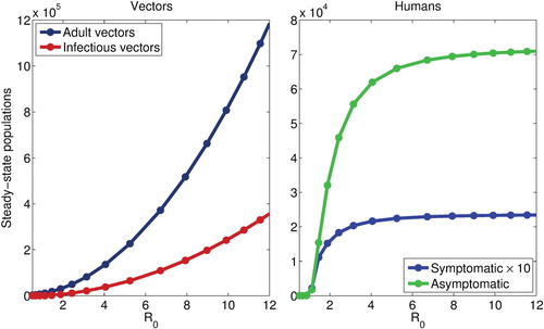
For the autonomous model, we plot the steady-state solution of the model for the total and infectious mosquito population, as well as the infected human populations (symptomatic and asymptomatic), against ${\mathcal{R}}_0$, revealing a quasi-linear relationship between ${\mathcal{R}}_0$ and the mosquito populations but a hyperbolic relationship between the human populations. The results obtained, depicted in Figure 4, suggest that, when ${\mathcal{R}}_0$ is relatively small, smaller changes in ${\mathcal{R}}_0$, whether due to changing climate or other factors, may significantly affect the burden of disease. However, when the baseline ${\mathcal{R}}_0$ is high, disease burden, but not the infectious vector population, is insensitive to such small changes. Thus, marginal changes in epidemiologic parameters and climate variables, such as temperature, are expected to significantly affect disease burden only in areas with a relatively low baseline ${\mathcal{R}}_0$.

Figure 4. Steady-state vector (total and infectious) and infected human populations (symptomatic and asymptomatic), as a function of ${\mathcal{R}}_0$, when the egg carrying capacity, $K_E$, is used to modulate ${\mathcal{R}}_0$ (similar results are obtained when other parameters are varied). Both vector populations increase super-linearly with ${\mathcal{R}}_0$, while a hyperbolic relationship between both infected human populations is seen, with little variation observed when ${\mathcal{R}}_0>4$. All other parameters values are as given in Table 3.

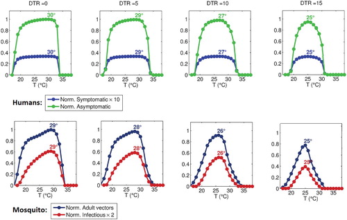
3.3. Temperature, ${\mathcal{R}}_0$, and endemic populations

For constant temperature, we may simply solve for ${\mathcal{R}}_0$ as a function of ambient temperature (using the thermal-response functions detailed in Section 2.6), yielding a unimodal curve, as seen in Figure 5. We may also simultaneously plot the endemic mosquito and infected human populations (under appropriate scaling), to see how this thermal-response function in ${\mathcal{R}}_0$ translates into disease burden.

Figure 5. Steady-state infectious vector (left panels) and infected human populations (right panels) as a function of ambient temperature, using either $K_E=2\times {10}^4$ (top panels) or $K_E=2\times {10}^5$ (bottom panels), with ${\mathcal{R}}_0$ normalized to the peak of either population also inscribed (the dotted line gives ${\mathcal{R}}_0\equiv 1$); peak ${\mathcal{R}}_0$ values are also indicated in the right panels. We see that infectious vectors track ${\mathcal{R}}_0$ quite well regardless, whereas infected human populations are nearly invariant when ${\mathcal{R}}_0$ is large across most of the temperature range where transmission is possible.

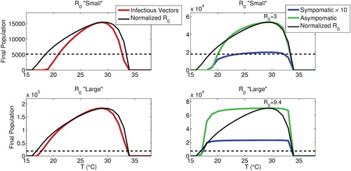
We see that this relationship depends upon the possible range for ${\mathcal{R}}_0$, as depicted in Figure 5, which shows how steady-state populations vary with temperature when ${\mathcal{R}}_0$ is relatively small versus large: When ${\mathcal{R}}_0$ is small over the temperature range where transmission is possible, infectious human populations also vary significantly, while when ${\mathcal{R}}_0$ is large over this temperature range, these populations are almost invariant, and the model tends to the same steady-state regardless. However, the infectious vector population still varies markedly with temperature even when ${\mathcal{R}}_0$ is large enough such that $I_H\left(\mathrm{\infty }\right)$ and $A_H\left(\mathrm{\infty }\right)$ do not. In all cases shown, ${\mathcal{R}}_0$ is modulated by $K_E$.

3.4. Sensitivity analysis

The model developed in this study contains numerous parameters. Hence, it is instructive to determine the model parameters that have the most influence on the disease transmission dynamics. To achieve this, a global sensitivity analysis, using latin hypercube sampling (LHS) and partial rank correlation coefficients (PRCC), is carried out to quantify the impact of the variations or sensitivity of each parameter of the model on the associated numerical simulations [16,56,58,100]. While PRCCs provide a measure of monotonicity after the removal of the linear effects of all but one variable [56], LHS, a stratified sampling without replacement technique, enables for the assessment of parameter variations across simultaneous uncertainty ranges in each parameter of the model. The sensitivity analysis is carried out for the autonomous model using the basic reproduction number (${\mathcal{R}}_0$) as the response function. The parameter values and ranges in Table 3 are used in this analysis, and it is assumed that each of the parameters of the model obey a uniform distribution [16,56]). The sensitivity analysis results obtained, tabulated in Table 4, show that the top PRCC-ranked parameters of the model are, in descending order, the aggregate (natural and biological control-related) death rate of adult female mosquitoes (${\mu }_M+{\eta }_M$), mosquito biting rate in stage I of the gonotrophic cycle ($b_H$), transmission probability from infected mosquitoes to susceptible humans $\left({\beta }_H\right)$, and the recovery rate for asymptomatically infected humans (${\alpha }_{HA})$. Thus, control strategies that increase the death rate of adult female mosquitoes (e.g., using indoor residual spraying), minimize biting rate (e.g., using long lasting insecticidal nets and other forms of personal protection against mosquito bite), and/or increase recovery of infected humans (e.g., via the use of artemisinin-based combination therapy) will be effective in reducing the disease burden in the community.

Table 4. PRCC values for the parameters of the autonomous model using the basic reproduction number ${\mathcal{R}}_0$ as the response function. The top (most-dominant) parameters that affect the dynamics of the model are highlighted in bold font. Parameter values and ranges used are as given in Table 3.

Parameters	PRCC	Parameters	PRCC	Parameters	PRCC	Parameters	PRCC
${\mathrm{\Pi }}_H$	$-0.18$	$b_H$	$\mathbf{+}\mathbf{0.57}$	${\beta }_H$	$\mathbf{+}\mathbf{0.53}$	${\gamma }_{HN}$	$+0.013$
${\mu }_H$	$-0.0234$	r	$-0.35$	${\nu }_H$	$+0.081$	${\delta }_H$	$+0.046$
${\delta }_{HA}$	$-0.034$	${\alpha }_{HA}$	$-0.44$	${\alpha }_H$	$-0.26$	${\psi }_E$	$+0.061$
${\sigma }_E$	$+0.32$	${\sigma }_{L_1}$	$+0.15$	${\sigma }_{L_2}$	$+0.17$	${\sigma }_{L_3}$	$+0.15$
${\sigma }_{L_4}$	$+0.12$	${\sigma }_P$	$+0.23$	f	$+0.13$	${\beta }_V$	$-0.42$
${\mu }_E+{\eta }_E$	$+0.15$	${\mu }_L+{\eta }_L$	$-0.15$	${\mu }_P+{\eta }_P$	$-0.034$	${\mu }_M+{\eta }_M$	$\mathbf{-}\mathbf{0.72}$
${\theta }_Y$	$+0.22$	${\varphi }_Z$	$-0.29$	${\kappa }_M$	$+0.34$	$K_E$	$+0.28$

4. Mathematical analysis of non-autonomous model

In this section, the full non-autonomous model $\left\{\right(1),(2),(3\left)\right\}$ will be analysed to gain insight into its dynamical features. It should be noted, first of all, that, as in the case of the autonomous model, the special case of the non-autonomous model with no density-dependent larval mortality (i.e., the model with $k_L=0$) has two disease-free equilibrium solutions, namely, the trivial disease-free equilibrium (${\mathcal{T}}_0$) and a non-trivial disease-free periodic solution (NDFS). Moreover, only NDFS will be analyzed (since the former, associated with the absence of mosquitoes in the population, is ecologically unrealistic). The non-trivial disease-free solution (denoted by ${\mathcal{E}}_N\left(t\right)$) exists whenever a vectorial reproduction ratio of the mosquito-only compartments, denoted by ${\mathcal{R}}_{Mt}$, exceeds unity (the detailed computation of ${\mathcal{R}}_{Mt}$, based on using the theory of linear operators [8,97], is given in Section 4.1 of [70], and not repeated here to save space). The NDFS is given by: (15) $\begin{array}{rl}{\mathcal{E}}_N\left(t\right)& =(\frac{{\mathrm{\Pi }}_H}{{\mu }_H},0,0,0,0,0,0,E^{\ast }\left(t\right),L_1^{\ast }\left(t\right),L_2^{\ast }\left(t\right),L_3^{\ast }\left(t\right),L_4^{\ast }\left(t\right),P^{\ast }\left(t\right),\\ & S_X^{\ast }\left(t\right),0,0,S_Y^{\ast }\left(t\right),0,0,S_Z^{\ast }\left(t\right),0,0),\end{array}$(15) where, $\left(E^{\ast }\right(t),L_1^{\ast }(t),L_2^{\ast }(t),L_3^{\ast }(t),L_4^{\ast }(t),P^{\ast }(t),S_X^{\ast }(t),0,0,S_Y^{\ast }(t),0,0,S_Z^{\ast }(t),0,0)$ is a periodic solution of the mosquito-only equivalent of the model at disease-free solution (i.e., they are periodic solutions of the model $\left\{\right(1),(2\left)\right\}$ only). The following stability results are obtained.

Theorem 4.1

1. Let ${\mathcal{R}}_{Mt}>1$. The NDFS of the non-autonomous model $\left\{\right(1),(2),(3\left)\right\}$, is locally-asymptotically stable whenever the threshold quantity ${\mathcal{R}}_{0t}<1$ and unstable if ${\mathcal{R}}_{0t}>1$.

2. Consider a special case of the non-autonomous model $\left\{\right(1),(2),(3\left)\right\}$ with ${\delta }_H={\delta }_{HA}=0$ (so that $N_H\left(t\right)\to {\mathrm{\Pi }}_H/{\mu }_H$ as $t\to \mathrm{\infty }$) and $k_L=0$. The NDFS of the resulting model is globally-asymptotically stable in $\mathrm{\Omega }\setminus \left\{{\mathcal{T}}_0\right\}$ if ${\mathcal{R}}_{1t}={\mathcal{R}}_{0t}{|}_{{\delta }_H={\delta }_R=k_L=0}\le 1$.

The proof of Item (1) of Theorem 4.1, based on using the theory of linear operators [8,70,97], is given in Appendix 3. The proof of Item (2) of Theorem 4.1, based on using the approach in [30,69], is given in Appendix 4. Thus, as in the case of the autonomous equivalent of the model (Theorem 3.2, the epidemiological implication of Theorem 4.1(2) is that, for the case of the non-autonomous model with no disease-induced mortality in the host population and no density-dependent larval mortality, malaria can be effectively controlled (or eliminated) from the community if the associated reproduction threshold (${\mathcal{R}}_{1t}$) can be brought to (and maintained at) a value less than unity. Thus, these analyses show that both the non-autonomous (with temperature fluctuations) model $\left\{\right(1),(2),(3\left)\right\}$ and its autonomous equivalent (where ambient temperature is fixed) have the same qualitative dynamics with respect to the local and global asymptotic dynamics of the associated non-trivial disease-free equilibrium (or solution).

4.1. Numerical simulations of non-autonomous model

The non-autonomous model $\left\{\right(1),(2),(3\left)\right\}$ is numerically simulated to illustrate the effect of temperature variability and diurnal temperature range (DTR) on malaria transmission dynamics. The temperature-dependent parameters are determined using the expressions given in Section 2.6 (for temperature values in the range $[14-40{]}^{\circ }$C, with daily variation about the mean given by Equation 8(8) $T_A\left(t\right)=T_{A0}-\frac{\mathrm{DTR}}{2}\sin [\frac{2\pi }{24}(t_h+14)],$(8) ). In addition, the effect of omitting explicit modelling of the gonotrophic and sprogonic cycles in the malaria transmission model is assessed.

4.1.1. Effect of daily temperature fluctuation

We run the model for various mean ambient temperatures, with superimposed (sinusoidal) diurnal temperature variation (as given by Equation 8(8) $T_A\left(t\right)=T_{A0}-\frac{\mathrm{DTR}}{2}\sin [\frac{2\pi }{24}(t_h+14)],$(8) ), with the DTR varying from 0${}^{\circ }$C to 15${}^{\circ }$C. The model is run until a stable periodic solution is reached, and the average values of this periodic solution are plotted against daily mean temperature for different values of DTR values, as shown in Figure 6. Results show that increasing DTR decreases both the possible temperature range for malaria transmission, and reduces the peak temperature value of maximum malaria transmission. Specifically, transmission is maximized at about 29.5${}^{\circ }$C when $\mathrm{DTR}=0^{\circ }$C (i.e., constant temperature), while peak transmission occurs at 25${}^{\circ }$C with $\mathrm{DTR}={15}^{\circ }$C, and indeed, at this point, transmission is already marginal at ${29.5}^{\circ }$C. Figure 6 shows that demonstrated that increasing DTR also asymmetrically narrows the temperature range over which malaria transmission is possible, such that transmission is curtailed somewhat more at higher, rather than lower, temperatures.

Figure 6. Approximate, normalized steady-state vector and infected human populations as functions of mean daily temperature, for DTR values of 0${}^{\circ }$C, 5${}^{\circ }$C, 10${}^{\circ }$C, and 15${}^{\circ }$C. Vector populations are normalized to the maximum total population under DTR of 0${}^{\circ }$C, while human populations are normalized to the maximum asymptomatic population under DTR of 0${}^{\circ }$C. All temperature-independent parameters are as in Table 3 except $K_E={10}^5$. Peak temperature value for all curves are indicated in the figure.

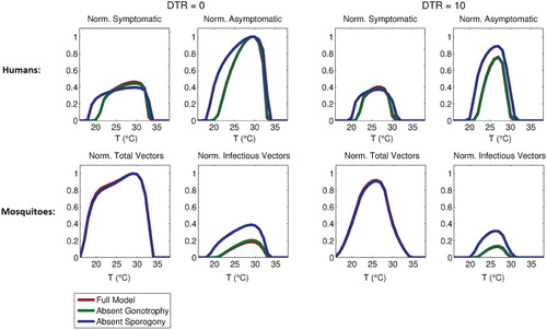
4.1.2. Omission of sporogonic and gonotropic cycles

The quantitative effect of the gonotrophic and sporogonic cycles on the malaria transmission model is assessed numerically by formulating two reduced version of the non-autonomous model, namely:

1. A reduced version of the non-autonomous model without an explicit representation of the adult female gonotrophic cycle;

2. A reduced version of the non-autonomous model without the exposed but non-infectious mosquito compartments (i.e., the model does not account for the delay from infection to infectivity imposed by the sporogonic cycle).

The resulting model equations are given in Appendix 5. Numerical simulations of the three models (i.e., the full model and the two reduced models), depicted in Figure 7, show that omitting the sporogonic cycle significantly affects the model output, but omitting the gonotrophic cycle has only a very marginal effect, when compared with the full model output.

Figure 7. Normalized steady-state of total adult vector, infectious vector, symptomatic human, and asymptomatic human populations for the full model and versions omitting either gonotrophy or sporogony cycles, as a function of daily mean temperature (with DTR values of 0${}^{\circ }$C and 10${}^{\circ }$C). Normalization is performed relative to the maximum total vector and asymptomatic human populations. All temperature-independent parameters are as given in Table 3, except $K_E={10}^4$.

5. Conclusions and discussion

We have developed and analyzed a deterministic non-autonomous (temperature-dependent) model for assessing the impact of temperature variability on the transmission dynamics of malaria in a community. In formulating the model, we considered several epidemiological features of malaria transmission including disease transmission to vectors by asymptomatically-infectious humans, reduced malaria susceptibility in humans due to recovery from prior malaria infection, the possibilities of conversion of symptomatic humans to an asymptomatic state, and the complete loss of partial immunity in humans. In addition to these features, the model explicitly incorporate the adult female gonotrophic cycle of the female Anopheles mosquitoes and the sporogonic cycle of the Plasmodium parasite.

The dynamics of the autonomous version of the model (where the ambient temperature is fixed) are governed by the basic reproduction number (${\mathcal{R}}_0$), which measures the average number of secondary cases of malaria caused by an infectious human (and vector) over the course of the infectious period, in an otherwise (wholly-susceptible) uninfected population. It is shown that, for the autonomous model, the disease-free equilibrium is locally-asymptotically stable whenever ${\mathcal{R}}_0<1$. The implication of this result is that the disease can be effectively controlled in the community, when ${\mathcal{R}}_0<1$, if the initial size of the infected population is small enough (in the basin of attraction of the disease-free equilibrium). It is further shown that this equilibrium is globally-asymptotically stable (when ${\mathcal{R}}_0<1$) for the special case with no disease-induced mortality in the host population. The epidemiological implication of the latter scenario is that making (and keeping) ${\mathcal{R}}_0$ to a value less than unity is necessary and sufficient for elimination of malaria in the community. Similar results were obtained for the full non-autonomous model (where daily temperature fluctuations are accounted for).

A global sensitivity analysis of the autonomous model, using Latin Hypercube Sampling and Partial Rank Correlation Coefficients, suggests that the dynamics of the model (with respect to ${\mathcal{R}}_0$ as the response function) are most sensitive to the net adult mosquito death rate (${\eta }_M+{\mu }_M$), biting rate ($b_H$) and human transmission probability (${\beta }_H$), and asymptomatic human recovery rate (${\alpha }_{HA}$). This suggests that the most effective malaria control measures will be those that target adult mosquito survival (increase ${\eta }_M$), such as indoor residual spraying (IRS) and widespread use of insecticide-treated bednets (ITNs) in the community, and block biting and transmission; ITNs are expected to decrease $b_H$, while ${\beta }_H$ may be reduced by, for instance, intermittent preventive therapy. Thus, this analysis is consistent with ITNs as a potentially highly effective measure. Effective medical treatment, including or even especially of those who are asymptomatic, is also likely to be of significant use. Targeting immature anophelines is likely to be of less efficacy than targeting adults, but still of value.

Several interesting observations arise from our numerical simulations of the autonomous model. First, there is a highly nonlinear, hyperbolic, relationship between ${\mathcal{R}}_0$ (which represents the average number of new infections generated by a single case in a completely susceptible, non-immune population, and the actual asymptotic populations of infected humans (both symptomatic and asymptomatic)), such that, once ${\mathcal{R}}_0$ is sufficiently large, disease burden is essentially unaffected by (reasonably small) changes in ${\mathcal{R}}_0$. This relates to the well-known fact about malaria epidemiology, namely that in highly endemic areas, the population may be exposed to as many as hundreds of infectious bites per year, yet disease burden is essentially stable, with most clinical disease concentrated in very young children who have not yet developed a degree of immunity [17]. It is only in more marginal areas of malaria transmission that disease burden tends to be more unstable, where severe disease affects persons across age groups and the population has a high degree of vulnerability to epidemics [17,54]. This is reflected in our model, in that only at relatively low ${\mathcal{R}}_0$ values do changes in this epidemiological quantity translate nearly linearly into clinical disease.

Furthermore, this phenomenon of ${\mathcal{R}}_0$ relating hyperbolically to clinical disease is also manifested in our ${\mathcal{R}}_0$-temperature curves. When temperature-independent parameters are such that ${\mathcal{R}}_0$ is relatively low across the temperature range for which transmission is possible, both ${\mathcal{R}}_0$ and infected human populations ($I_H$ and $A_H$) change appreciably with temperature. If, on the other hand, the “basal” ${\mathcal{R}}_0$ is high, then while ${\mathcal{R}}_0$ changes with temperature, $I_H$ and $A_H$ do not, except for a quasi-threshold phenomenon where, below about 17 and above 34${}^{\circ }$C, $I_H$ and $A_H$ are zero, but almost invariant within these temperature bounds. Thus, our results suggest that climate change may affect areas of high malaria endemicity (e.g. holo- and hyperendemic areas) and areas of low endemicity or unstable transmission very differently. Within the former, which tend to be warm areas in western and central equatorial Africa, several degrees of warming will affect disease burden only if a threshold mean daily temperature (likely on the order of about 34${}^{\circ }$C) is crossed, and then dramatically, with a sharp drop in disease burden. In the latter, which tend to be cooler areas, such as the eastern African highlands, warming temperatures may affect disease burden in a more continuous manner, with increases in ${\mathcal{R}}_0$ with temperature translating more directly into clinical disease. Thus, modest warming would most likely result in a net increase in overall disease potential.

Numerical simulations also indicate that temperature variability is important in determining the optimum temperature ranges for malaria transmission, with increasing daily temperature range (DTR) shifting the optimum temperature for transmission down from about 29.5${}^{\circ }$C when temperature is constant, to 23.5${}^{\circ }$C when DTR is 20${}^{\circ }$C, and moreover, asymmetrically contracting the temperature range where transmission is possible, such that higher temperatures are more affected, in reasonable concordance with recent modelling work by Beck-Johnson et al. [13].

Finally, given the complexity and large number of variables in the full transmission model considered here, we have briefly analyzed two reduced models, one omitting explicit representation of the gonotrophic cycle and the other omitting the sporogonic cycle. In the former case, normalized asymptotic mosquito and infected humans populations are hardly affected under constant weather conditions, although dynamics may still be affected when weather conditions vary. The omission of sporogony, however, very strongly affects model predictions, and is likely essential to include. It follows that it may be a reasonable to simplify future models by omitting explicit disaggregation of the gonotrophic cycle into compartments, but this is likely untrue for the sporogonic cycle.

Disclosure statement

No potential conflict of interest was reported by the authors.

Additional information

Funding

One of the authors (ABG) is grateful to National Institute for Mathematical and Biological Synthesis (NIMBioS) for funding the Working Group on Climate Change and Vector-borne Diseases (VBDs). NIMBioS is an Institute sponsored by the National Science Foundation, the U.S. Department of Homeland Security, and the U.S. Department of Agriculture through NSF Award #EF-0832858, with additional support from The University of Tennessee, Knoxville. The authors acknowledge the support, in part, of the Simons Foundation (Award $\mathrm{\#}$585022). The authors are grateful to the two anonymous reviewers for their very insightful and constructive comments.

Appendix 1. Proof of Lemma 2.1

Proof.

Since the functions on the right-hand side of the model $\left\{\right(1),(2),(3\left)\right\}$ (denoted by $Q(t,\phi )$, where $\phi \in {\mathbb{R}}_{+}^{22}$) is continuous and Lipschitzian at t=0, then for each non-negative initial condition, the model has a unique and non-negative solution in ${\mathbb{R}}_{+}^{22}$. In addition, it should be noted that $Q_i(t,\phi )\ge 0$ whenever $\phi \ge 0$ and ${\phi }_i=0$. Hence, it follows from Theorem A.4 in [95] that the region ${\mathbb{R}}_{+}^{22}$ is positively-invariant with respect to the model $\left\{\right(1),(2),(3\left)\right\}$. Furthermore, consider the following definition,

Definition A.1

For each of the time-dependent (i.e., temperature- and rainfall-dependent) parameters, the following quantities hold: $a^{\ast }=\underset{t\ge 0}{sup}a\left(t\right),a_{\ast }=\underset{t\ge 0}{inf}a\left(t\right)$

Using Definition A.1, the boundedness of the solutions of the model $\left\{\right(1),(2),(3\left)\right\}$ is shown as follows:

1. Immature and adult mosquito compartments:

   Since $(1-(E/K_E){)}_{+}\ge 0$, then $E\left(t\right)\le K_E$ for all t. Thus, using Definition A.1, it can be deduced from the second equation of immature mosquito compartments (i.e., using the equation for the first larval instar stage ($L_1$) described in Section 2.2) that, $\frac{\mathrm{d}{L}_1}{\mathrm{d}t}={\sigma }_E\left(t\right)E-\left[{\sigma }_{L_1}\right(t)+{\eta }_L+k_{L}L+{\mu }_L(t\left)\right]L_1\le {\sigma }_E^{\ast }{K}_E-({\sigma }_{L_{1\ast }}+{\eta }_L+{\mu }_{L\ast })L_1,$ so that $\underset{t\to \mathrm{\infty }}{lim sup}{L}_1\left(t\right)\le {\sigma }_E^{\ast }{K}_E/\left({\sigma }_{L_{1\ast }}+{\eta }_L+{\mu }_{L\ast }\right)={\overline{L}}_1.$ Similarly, the following bounds are obtained: $\underset{t\to \mathrm{\infty }}{lim sup}{L}_j\left(t\right)\le {\overline{L}}_j={\displaystyle \frac{{\sigma }_{L_{(j-1)}}^{\ast }{L}_{j-1}}{{\sigma }_{L_j\ast }+{\eta }_L+{\mu }_{L\ast }}}(\mathrm{for}j=2,3,4)\mathrm{and}\underset{t\to \mathrm{\infty }}{lim sup}P\left(t\right)\le \overline{P}={\displaystyle \frac{{\sigma }_{L_4}^{\ast }{L}_4}{{\sigma }_{P\ast }+{\eta }_P+{\mu }_P}}$.

   Furthermore, the equation for the rate of change of the total adult mosquitoes population ($N_V\left(t\right)$) is given by: $\frac{\mathrm{d}{N}_V}{\mathrm{d}t}=f{\sigma }_P\left(t\right)P-[{\eta }_M+{\mu }_M(t\left)\right]N_V\le f{\sigma }_P^{\ast }\overline{P}-({\eta }_M+{\mu }_{M\ast })N_V.$ from which it follows that $\underset{t\to \mathrm{\infty }}{lim sup}{N}_V\left(t\right)\le f{\sigma }_P^{\ast }\overline{P}\left({\eta }_M+{\mu }_{M\ast }\right)={\overline{N}}_V.$

2. Human compartments:

   The equation for the rate of change of the total human population ($N_H\left(t\right)$): $\frac{\mathrm{d}{N}_H}{\mathrm{d}t}={\mathrm{\Pi }}_H-{\mu }_H{N}_H\left(t\right)-{\delta }_{HA}{A}_H\left(t\right)-{\delta }_H{I}_H\left(t\right)\le {\mathrm{\Pi }}_H-{\mu }_H{N}_H\left(t\right),$ so that $N_H\left(t\right)={\mathrm{\Pi }}_H/{\mu }_H+\left[N_H\right(0)-({\mathrm{\Pi }}_H/{\mu }_H\left)\right]{\mathrm{e}}^{-{\mu }_{H}t}.$ Thus, $N_H\le {\mathrm{\Pi }}_H/{\mu }_H$ if $N_H\left(0\right)\le {\mathrm{\Pi }}_H/{\mu }_H$. In addition, if $N_H\left(0\right)>{\mathrm{\Pi }}_H/{\mu }_H$, then $N_H\left(t\right)\to {\mathrm{\Pi }}_H/{\mu }_H$ as $t\to \mathrm{\infty }$. That is, $\underset{t\to \mathrm{\infty }}{lim sup}\le {\mathrm{\Pi }}_H/{\mu }_H$.

Appendix 2. Proof of Theorem 3.2

Proof.

Consider the special case of the autonomous model with ${\delta }_H={\delta }_{HA}=0$ so that $N_H\left(t\right)\to N_H^{\ast }={\mathrm{\Pi }}_H/{\mu }_H$, as $t\to \mathrm{\infty }$. Furthermore, let $k_L=0$ and ${\mathcal{R}}_{MP}>1$ (so that the unique NDFE, ${\mathcal{E}}_0$, exists) and ${\mathcal{R}}_1={\mathcal{R}}_0{|}_{{\delta }_H={\delta }_{HA}=0}<1$. Following [30,69], it is convenient to re-write the autonomous model (A1) $\begin{array}{rl}\frac{\mathrm{d}{x}_S}{\mathrm{d}t}& =A_1\left(x\right)(x_S-x_{NDFE,S})+A_{12}\left(x\right)x_I,\\ \frac{\mathrm{d}{x}_I}{\mathrm{d}t}& =A_2\left(x\right)x_I,\end{array}$(A1) where, $\begin{array}{rl}{x}_S\left(t\right)& =(S_H\left(t\right),W_H\left(t\right),R_H\left(t\right),E\left(t\right),L_1\left(t\right),L_2\left(t\right),L_3\left(t\right),L_4\left(t\right),P\left(t\right),S_X\left(t\right),S_Y\left(t\right),S_Z\left(t\right){)}^T,\\ x_I\left(t\right)& =(E_{HN}\left(t\right),E_{HR}\left(t\right),I_H\left(t\right),A_H\left(t\right),E_X\left(t\right),I_X\left(t\right),E_Y\left(t\right),I_Y\left(t\right),E_Z\left(t\right),I_Z\left(t\right),0,0{)}^T,\\ x_{NDFE,S}& =(S_H^{\diamond },0,0,E^{\diamond },L_1^{\diamond },L_2^{\diamond },L_3^{\diamond },L_4^{\diamond },P_V^{\diamond },S_X^{\diamond },S_Y^{\diamond },S_Z^{\diamond }{)}^T,\end{array}$ $\begin{array}{rl}{A}_1\left(x\right)& =\left[\begin{array}{cccccc}-{\mu }_H& +{\rho }_H& 0& 0& 0& 0\\ 0& -({\rho }_H+{\mu }_H)& {\xi }_H& 0& 0& 0\\ 0& 0& -({\xi }_H+{\mu }_H)& 0& 0& 0\\ 0& 0& 0& -g_E-{\psi }_E{\varphi }_Z\frac{S_Z}{K_E}& 0& 0\\ 0& 0& 0& {\sigma }_E& -g_{L1}& 0\\ 0& 0& 0& 0& {\sigma }_{L_1}& -g_{L2}\\ 0& 0& 0& 0& 0& {\sigma }_{L_2}\\ 0& 0& 0& 0& 0& 0\\ 0& 0& 0& 0& 0& 0\\ 0& 0& 0& 0& 0& 0\\ 0& 0& 0& 0& 0& 0\\ 0& 0& 0& 0& 0& 0\end{array}\right.\\ & \left.\begin{array}{cccccc}0& 0& 0& 0& 0& 0\\ 0& 0& 0& 0& 0& 0\\ 0& 0& 0& 0& 0& 0\\ 0& 0& 0& 0& 0& {\psi }_E{\varphi }_Z(1-\frac{E^{\diamond }}{K_E})\\ 0& 0& 0& 0& 0& 0\\ 0& 0& 0& 0& 0& 0\\ -g_{L3}& 0& 0& 0& 0& 0\\ {\sigma }_{L_3}& -g_{L2}& 0& 0& 0& 0\\ 0& {\sigma }_{L_4}& -g_P& 0& 0& 0\\ 0& f{\sigma }_P& -C_X& 0& 0& 0\\ 0& 0& 0& b_H(1-{\beta }_V{\mathcal{G}}_H)& -C_Y& 0\\ 0& 0& 0& 0& {\theta }_Y& -C_Z\end{array}\right],\end{array}$ $\begin{array}{r}{A}_{12}\left(x\right)=\left[\begin{array}{cccccccccccc}0& 0& 0& 0& 0& b_H{\beta }_H\frac{S_H}{N_H}& 0& 0& 0& 0& 0& 0\\ 0& 0& 0& 0& 0& (1-ϵ)b_H{\beta }_H\frac{W_H}{N_H}& 0& 0& 0& 0& 0& 0\\ 0& 0& {\alpha }_H& {\alpha }_{HA}& 0& 0& 0& 0& 0& 0& 0& 0\\ 0& 0& 0& 0& 0& 0& 0& 0& {\psi }_E{\varphi }_Z(1-\frac{E}{K_E})& {\psi }_E{\varphi }_Z(1-\frac{E}{K_E})& 0& 0\\ 0& 0& 0& 0& 0& 0& 0& 0& 0& 0& 0& 0\\ 0& 0& 0& 0& 0& 0& 0& 0& 0& 0& 0& 0\\ 0& 0& 0& 0& 0& 0& 0& 0& 0& 0& 0& 0\\ 0& 0& 0& 0& 0& 0& 0& 0& 0& 0& 0& 0\\ 0& 0& 0& 0& 0& 0& 0& 0& 0& 0& 0& 0\\ 0& 0& 0& 0& 0& 0& 0& 0& 0& 0& 0& 0\\ 0& 0& 0& 0& 0& 0& 0& 0& 0& 0& 0& 0\\ 0& 0& 0& 0& 0& 0& 0& 0& 0& 0& 0& 0\end{array}\right],\end{array}$and, $\begin{array}{rl}{A}_2\left(x\right)& =\left[\begin{array}{ccccc}-g_1& 0& 0& 0& 0\\ 0& -g_2& 0& 0& 0\\ r{\gamma }_{HN}& q{\gamma }_{HR}& -g_3& 0& 0\\ (1-r){\gamma }_{HN}& (1-q){\gamma }_{HR}& {\nu }_H& -g_4& 0\\ 0& 0& 0& 0& -g_X\\ 0& 0& 0& 0& {\kappa }_M\\ 0& 0& b_H{\beta }_V\frac{S_X}{N_H}& b_H{\beta }_V\frac{S_X}{N_H}& b_H\\ 0& 0& 0& 0& 0\\ 0& 0& 0& 0& 0\\ 0& 0& 0& 0& 0\\ 0& 0& 0& 0& 0\\ 0& 0& 0& 0& 0\end{array}\right.\\ & \left.\begin{array}{ccccccc}{b}_H{\beta }_H\frac{S_H}{N_H}& 0& 0& 0& 0& 0& 0\\ (1-ϵ)b_H{\beta }_H\frac{W_H}{N_H}& 0& 0& 0& 0& 0& 0\\ 0& 0& 0& 0& 0& 0& 0\\ 0& 0& 0& 0& 0& 0& 0\\ 0& 0& 0& 0& 0& 0& 0\\ -C_X& 0& 0& 0& 0& 0& 0\\ 0& -g_Y& 0& 0& 0& 0& 0\\ b_H& {\kappa }_M& -C_Y& 0& 0& 0& 0\\ 0& {\theta }_Y& 0& -g_Z& 0& 0& 0\\ 0& 0& {\theta }_Y& {\kappa }_M& -C_Z& 0& 0\\ 0& 0& 0& 0& 0& 0& 0\\ 0& 0& 0& 0& 0& 0& 0\end{array}\right],\end{array}$with $g_1={\gamma }_{HN}+{\mu }_H$, $g_2={\gamma }_{HR}+{\mu }_H$, $g_3={\alpha }_H+{\nu }_H+{\delta }_H+{\mu }_H$, $g_4={\alpha }_{HA}+{\delta }_{HA}+{\mu }_H$, $C_X=b_H+{\eta }_M+{\mu }_M$, $C_Y={\theta }_Y+{\eta }_M+{\mu }_M$, $C_Z={\varphi }_Z+{\eta }_M+{\mu }_M$, $g_X=C_X+{\kappa }_M$, $g_Y=C_Y+{\kappa }_M$ and $g_Z=C_Z+{\kappa }_M$. It can be verified that the eigenvalues of $A_1\left(x\right)$ are real and non-positive. Hence, the system $\mathrm{d}{x}_S/\mathrm{d}t=A_1\left(x\right)(x_S-x_{NDFE,S})$ is globally-asymptotically stable at $x_{NDFE,S}$ [30]. It should be noted that the matrix $A_2\left(x\right)$ is a Metzler irreducible. Consider, next, the following bounded invariant set: $\begin{array}{rl}{\mathcal{B}}_2& =\{(S_H,W_H,R_H,E,L_1,L_2,L_3,L_4,P,S_X,S_Y,S_Z,E_{HN},E_{HR},I_H,A_H,E_X,I_X,E_Y,I_Y,E_Z,I_Z,\\ & 0,0)\in {\mathbb{R}}_{+}^{24}:N_H\le \frac{{\mathrm{\Pi }}_H}{{\mu }_H},N_V\le {\overline{N}}_V\},\end{array}$ It is convenient to define $({\mathcal{R}}_G{)}^2=\frac{{\overline{N}}_V}{S_X^{\diamond }}({\mathcal{R}}_1{)}^2>({\mathcal{R}}_1{)}^2.$ Further, define a matrix $A_2\left(\overline{x}\right)=\overline{A_2}$, where $\overline{A_2}$ is an upper bound of the set [16] $\mathcal{M}=\{A_2\left(x\right)\in {\mathbb{R}}^{12\times 12}:x\left(t\right)\in {\mathcal{B}}_2\},$ with $\overline{x}\in {\mathbb{R}}_{+}^{12}\times \left\{0\right\}$. It can be verified that $\rho \left(\overline{A_2}\right)\le 0$ if and only if ${\mathcal{R}}_G\le 1$. Thus, it follows from Theorem 2.7 in [30] that, for ${\mathcal{R}}_{MP}>1$ and ${\mathcal{R}}_1<1$, (A2) $\begin{array}{rl}& (S_H,W_H,R_H,E,L_1,L_2,L_3,L_4,P,S_X,S_Y,S_Z,E_{HN},E_{HR},I_H,A_H,E_X,I_X,E_Y,I_Y,E_Z,I_Z)\left(t\right)\\ & \to (\frac{{\mathrm{\Pi }}_H}{{\mu }_H},0,0,E^{\diamond },L_1^{\diamond },L_2^{\diamond },L_3^{\diamond },L_4^{\diamond },P^{\diamond },S_X^{\diamond },S_Y^{\diamond },S_Z^{\diamond },0,0,0,0,0,0,0,0,0,0),\mathrm{as}t\to \mathrm{\infty },\end{array}$(A2) where $E^{\diamond },L_1^{\diamond },L_2^{\diamond },L_3^{\diamond },L_4^{\diamond },P^{\diamond },S_X^{\diamond },S_Y^{\diamond },S_Z^{\diamond }$ are as defined in Equation (9(9) $\begin{array}{rl}& E_V^{\diamond }=K_E(1-\frac{1}{{\mathcal{R}}_{MP}}),L_1^{\diamond }=\frac{{\sigma }_E}{C_{L1}}{E}^{\diamond },L_j^{\diamond }=\frac{{\sigma }_{L_{j-1}}}{C_{Lj}}{L}_{j-1}^{\diamond },j=2,3,4,\\ & P_V^{\diamond }=\frac{{\sigma }_{L_4}}{C_P}{L}_4^{\diamond },\\ & S_X^{\diamond }=\frac{1}{C_X}(f{\sigma }_P{P}^{\diamond }+{\varphi }_Z{S}_Z^{\diamond }),S_Y^{\diamond }=\frac{1}{C_Y}{b}_H{S}_X^{\diamond },S_Z^{\diamond }=\frac{{\theta }_Y{b}_{H}f{\sigma }_P{P}^{\diamond }}{C_X{C}_Y{C}_Z-{\theta }_Y{b}_H{\varphi }_Z},\end{array}$(9) ) in Section 3.1. Thus, the unique NDFE (${\mathcal{E}}_0$) of the autonomous model, with ${\delta }_H={\delta }_{HA}=0$, is globally-asymptotically stable in $\mathrm{\Omega }\setminus \left\{{\mathcal{T}}_0\right\}$ whenever ${\mathcal{R}}_1<1$.

Appendix 3. Proof of Theorem 4.1(1)

Proof.

Computation of ${\mathcal{R}}_{0t}$: The vectorial reproduction ratio, associated with the non-autonomous model $\left\{\right(1),(2),(3\left)\right\}$, will be computed using the approach in [8,70,97]. The linearized version of the model $\left\{\right(1),(2),(3\left)\right\}$, at the disease-free solution, ${\mathcal{E}}_N\left(t\right)$, can be expressed as (A3) $\frac{\mathrm{d}\mathcal{H}\left(t\right)}{\mathrm{d}t}=[\mathcal{F}\left(t\right)-\mathcal{V}\left(t\right)]\mathcal{H}\left(t\right)$(A3) where $\mathcal{H}=(E_{HN},E_{HR},I_H,A_H,E_X,I_X,E_Y,I_Y,E_Z,I_Z)$, $\mathcal{F}\left(t\right)$ and $\mathcal{V}\left(t\right)$, are the next generation matrices (of the new infections and remaining transfer terms, respectively) associated with the model$\left\{\right(1),(2),(3\left)\right\}$ when linearized at the trivial equilibrium ${\mathcal{E}}_N\left(t\right)$.

Furthermore, the cumulative distribution of new infections at time t, produced by all infected individuals introduced at a prior time s=t, is given by $\mathrm{\Psi }\left(t\right)={\int }_{-\mathrm{\infty }}^{t}Y(t,s)\mathcal{F}\left(s\right)\phi \left(s\right)\mathrm{d}s={\int }_0^{\mathrm{\infty }}Y(t,t-a)\mathcal{F}(t-a)\phi (t-a)\mathrm{d}a.$ where, $Y(t,s)$ is the matrix of evolution operator of the linear ω-periodic system which satisfies [97] $\frac{\mathrm{d}Y(t,s)}{\mathrm{d}t}=-\mathcal{V}\left(t\right)Y_M(t,s)\mathrm{\forall }t\ge s,Y(s,s)=I,$ and $\phi \left(s\right)$ (ω-periodic in s) is the initial distribution of infectious individuals, so that $\mathcal{F}\left(s\right)\phi \left(s\right)$ is the rate at which new infections are produced by infected individuals who were introduced into the population at time s; and $Y(t,s)\mathcal{F}\left(s\right)\phi \left(s\right)$ represents the distribution of those infected individuals who were newly-infected at time s, and remain infected at time t.

The threshold quantity (${\mathcal{R}}_{0t}$), is the spectral radius of the linear operator L defined by $L:{\mathbb{C}}_{\omega }\to {\mathbb{C}}_{\omega }$ [97], with $\left(L\phi \right)\left(t\right)={\int }_0^{\mathrm{\infty }}Y(t,t-a)\mathcal{F}(t-a)\phi (t-a)\mathrm{d}a\mathrm{\forall }t\in \mathbb{R},\phi \in {\mathbb{C}}_{\omega }.$ where ${\mathbb{C}}_{\omega }$ is the ordered Banach space of all ω-periodic functions from $\mathbb{R}$ to ${\mathbb{R}}^{22}$, which is equipped with maximum norm and positive cone ${\mathbb{C}}_{\omega }^{+}\{\phi \in {\mathbb{C}}_{\omega }:\phi (t)\ge 0,\mathrm{\forall }t\in \mathbb{R}\}$ [97]. In addition, tt can be verified that system $\left\{\right(1),(2),(3\left)\right\}$ satisfy the assumptions A1−A7 in [97]. Hence, the result of Theorem 4.1 follows from Theorem 2.2 in [97].

Appendix 4. Proof of Theorem 4.1(2)

Proof.

In the case where ${\mathcal{R}}_{Mt}>1$ and ${\mathcal{R}}_{0t}<1$, Theorem 4.1(1) implies that the disease-free periodic state ${\mathcal{E}}_N\left(t\right)$ is locally asymptotically stable. We now show that it attracts all non-negative solutions of model $\left\{\right(1),(2),(3\left)\right\}$.

Using a standard comparison argument [48], it can be verified that an upper bound of the linearizing system (i.e., the non-autonomous model linearized at the disease-free periodic state), is given by Equation (A3(A3) $\frac{\mathrm{d}\mathcal{H}\left(t\right)}{\mathrm{d}t}=[\mathcal{F}\left(t\right)-\mathcal{V}\left(t\right)]\mathcal{H}\left(t\right)$(A3) ) in Appendix C. Thus, it suffices to show that every solution of Equation (A3(A3) $\frac{\mathrm{d}\mathcal{H}\left(t\right)}{\mathrm{d}t}=[\mathcal{F}\left(t\right)-\mathcal{V}\left(t\right)]\mathcal{H}\left(t\right)$(A3) ), converges to zero as $t\to \mathrm{\infty }$.

It follows from Lemma 2.1 in [104] that there exists a positive τ-periodic function, $\hat{\mathcal{H}}\left(t\right)$, such that $\mathcal{H}\left(t\right)={\mathrm{e}}^{pt}\hat{\mathcal{H}}\left(t\right)$ is a solution of Equation (A3(A3) $\frac{\mathrm{d}\mathcal{H}\left(t\right)}{\mathrm{d}t}=[\mathcal{F}\left(t\right)-\mathcal{V}\left(t\right)]\mathcal{H}\left(t\right)$(A3) ), where $p=1/\tau \ln \rho \left({\mathrm{\Phi }}_{\mathcal{F}\left(t\right)-\mathcal{V}\left(t\right)}\right(\tau \left)\right)$. Furthermore, by Theorem 2.2 in [104], it follows that for ${\mathcal{R}}_{Mt}>1$ and ${\mathcal{R}}_{0t}<1$, $\rho \left({\mathrm{\Phi }}_{\mathcal{F}\left(t\right)-\mathcal{V}\left(t\right)}\right(\tau \left)\right)$ and p<0 (so that $\mathcal{H}\left(t\right)\to 0$ as $t\to \mathrm{\infty }$). Therefore, the zero solution of Equation (A3(A3) $\frac{\mathrm{d}\mathcal{H}\left(t\right)}{\mathrm{d}t}=[\mathcal{F}\left(t\right)-\mathcal{V}\left(t\right)]\mathcal{H}\left(t\right)$(A3) ) is globally asymptotically stable. Furthermore, substituting the zero solution of Equation (A3(A3) $\frac{\mathrm{d}\mathcal{H}\left(t\right)}{\mathrm{d}t}=[\mathcal{F}\left(t\right)-\mathcal{V}\left(t\right)]\mathcal{H}\left(t\right)$(A3) ) (i.e., $(E_{HN},E_{HR},I_H,A_H,E_X,I_X,E_Y,I_Y,E_Z,I_Z)\left(t\right)\to (0,0,\dots ,0)$) into the non-autonomous model $\left\{\right(1),(2),(3\left)\right\}$ shows that the non-trivial disease-free periodic solution ${\mathcal{E}}_N\left(t\right)$ (given by (15(15) $\begin{array}{rl}{\mathcal{E}}_N\left(t\right)& =(\frac{{\mathrm{\Pi }}_H}{{\mu }_H},0,0,0,0,0,0,E^{\ast }\left(t\right),L_1^{\ast }\left(t\right),L_2^{\ast }\left(t\right),L_3^{\ast }\left(t\right),L_4^{\ast }\left(t\right),P^{\ast }\left(t\right),\\ & S_X^{\ast }\left(t\right),0,0,S_Y^{\ast }\left(t\right),0,0,S_Z^{\ast }\left(t\right),0,0),\end{array}$(15) ) in Section 4) is the unique periodic solution (for ${\mathcal{R}}_{Mt}>1$). By the comparison principle [91] and the theory of asymptotic autonomous systems [94], ${\mathcal{R}}_{0t}<1$, then ${\mathcal{E}}_N\left(t\right)$ is globally attractive. Therefore, ${\mathcal{E}}_N\left(t\right)$ is globally-asymptotically stable.

Appendix 5. Equations of Reduced Models: Omission of Gonotrophic or Sporogonic Cycle

A.1. Gonotrophic cycle omitted

Adult female model equations without explicit modeling of the gonotrophic cycle. (A4) $\begin{array}{rl}\frac{\mathrm{d}{S}_X}{\mathrm{d}t}& =f{\sigma }_{P}P-[\mathrm{\Gamma }{b}_H{\beta }_V{\mathcal{G}}_H+{\eta }_M+{\mu }_M\left(t\right)]S_X,\\ \frac{\mathrm{d}{E}_X}{\mathrm{d}t}& =\mathrm{\Gamma }{b}_H{\beta }_V{\mathcal{G}}_H{S}_X-[{\kappa }_M\left(t\right)+{\eta }_M+{\mu }_M\left(t\right)]E_X,\\ \frac{\mathrm{d}{I}_X}{\mathrm{d}t}& ={\kappa }_M\left(t\right)E_X-[{\eta }_M+{\mu }_M\left(t\right)]I_X,\end{array}$(A4) where Γ is the overall biting rate (the inverse of the gonotrophic cycle length [61]), in days⁻¹, given by $\mathrm{\Gamma }=\left(\right(1/b_H)+(1/{\varphi }_Z)+(1/{\theta }_Y){)}^{-1}$, and the infection rate of susceptible humans (by $I_X$) in the resulting model, is given by ${\lambda }_H=\mathrm{\Gamma }{\beta }_H\left(I_X/N_H\right).$

A.2. Sporogonic cycle omitted

Adult female compartments in the absence of the Plasmodium's sporogonic cycle (A5) $\begin{array}{rl}\frac{\mathrm{d}{S}_X}{\mathrm{d}t}& =f{\sigma }_{P}P+{\varphi }_Z{S}_Z-[b_H+{\eta }_M+{\mu }_M\left(t\right)]S_X,\\ \frac{\mathrm{d}{I}_X}{\mathrm{d}t}& ={\varphi }_Z{I}_Z-[b_H+{\eta }_M+{\mu }_M\left(t\right)]I_X,\\ \frac{\mathrm{d}{S}_Y}{\mathrm{d}t}& =b_H(1-{\beta }_V){\mathcal{G}}_H{S}_X+b_H(1-{\mathcal{G}}_H)S_X-[{\theta }_Y\left(t\right)+{\eta }_M+{\mu }_M\left(t\right)]S_Y,\\ \frac{\mathrm{d}{I}_Y}{\mathrm{d}t}& =b_H{\beta }_V{\mathcal{G}}_H{S}_X+b_H{I}_X-[{\theta }_Y\left(t\right)+{\eta }_M+{\mu }_M\left(t\right)]I_Y,\\ \frac{\mathrm{d}{S}_Z}{\mathrm{d}t}& ={\theta }_Y\left(t\right)S_Y-[{\varphi }_Z+{\eta }_M+{\mu }_M\left(t\right)]S_Z,\\ \frac{\mathrm{d}{I}_Z}{\mathrm{d}t}& ={\theta }_Y\left(t\right)I_Y-[{\varphi }_Z+{\eta }_M+{\mu }_M\left(t\right)]I_Z.\end{array}$(A5) ${\mathcal{G}}_H=\left(I_H+A_H\right)/N_H$ for both cases.

References

- J.L. Aron, Mathematical modelling of immunity to malaria, Math. Biosci. 90 (1988), pp. 385–396. doi: 10.1016/0025-5564(88)90076-4
- A. Abdelrazec and A.B. Gumel, Mathematical assessment of the role of temperature and rainfall on mosquito population dynamics, J. Math. Bio. 74 (2017), pp. 1351–1395. doi: 10.1007/s00285-016-1054-9
- Y.A. Afrane, B.W. Lawson, A.K. Githeko, and G. Yan, Effects of microclimatic changes caused by land use and land cover on duration of gonotrophic cycles of Anopheles gambiae (Diptera: Culicidae) in western Kenya highlands, J. Med. Entomol. 42 (2005), pp. 974–980. doi: 10.1093/jmedent/42.6.974
- F.B. Agusto, A.B. Gumel, and P.E. Parham, Qualitative assessment of the role of temperature variations on malaria transmission dynamics, J. Biol. Syst. 23 (2015), p. 1550030. doi: 10.1142/S0218339015500308
- H.K. Alles, K.N. Mendis, and R. Carter, Malaria mortality rates in South Asia and in Africa: Implications for malaria control, Parasitol. Today 14 (1998), pp. 369–375. doi: 10.1016/S0169-4758(98)01296-4
- S. Antinori, L. Galimberti, L. Milazzo, and M. Corbellino, Biology of human malaria plasmodia including Plasmodium knowlesi, Mediterr. J. Hematol. Infect. Dis. 4 (2012), p. 2012013. doi: 10.4084/mjhid.2012.013
- E.A. Ashley and N.J. White, The duration of Plasmodium falciparum infections, Malar. J. 13 (2014), p. 500. doi: 10.1186/1475-2875-13-500
- N. Bacaër, Approximation of the basic reproduction number R0 for vector-borne diseases with a periodic vector population, Bull. Math. Biol. 69 (2007), pp. 1067–1091. doi: 10.1007/s11538-006-9166-9
- M.N. Bayoh, Studies on the development and survival of Anopheles gambiae sensu stricto at various temperatures and relative humidities, Doctoral diss., Durham Theses, Durham University, 2001. Available at http://etheses.dur.ac.uk/4952/.
- M.N. Bayoh and S.W. Lindsay, Effect of temperature on the development of the aquatic stages of Anopheles gambiae sensu stricto (Diptera: Culicidae), Bull. Entomol. Res. 93 (2003), pp. 375–381. doi: 10.1079/BER2003259
- M.N. Bayoh and S.W. Lindsay, Temperature-related duration of aquatic stages of the Afrotropical malaria vector mosquito Anopheles gambiae in the laboratory, Med. Vet. Entomol. 18 (2004), pp. 174–179. doi: 10.1111/j.0269-283X.2004.00495.x
- L.M. Beck-Johnson, W.A. Nelson, K.P. Paaijmans, A.F. Read, M.B. Thomas, and O.N. Bjørnstad, The effect of temperature on Anopheles mosquito population dynamics and the potential for malaria transmission, PLoS One 8(11) (2013), p. e79276. doi: 10.1371/journal.pone.0079276
- L.M. Beck-Johnson, W.A. Nelson, K.P. Paaijmans, A.F. Read, M.B. Thomas, and O.N. Bjørnstad, The importance of temperature fluctuations in understanding mosquito population dynamics and malaria risk, R. Soc. Open Sci. 4 (2017), p. 160969. doi:10.1098/rsos.160969.
- S.E. Bellan, The importance of age dependent mortality and the extrinsic incubation period in models of mosquito-borne disease transmission and control, PLoS One 5 (2010), p. e10165. doi: 10.1371/journal.pone.0010165
- S. Bhattacharya, C. Sharma, R.C. Dhiman, and A.P. Mitra, Climate change and malaria in India, Curr. Sci. 90(3) (2006), pp. 369–375.
- S.M. Blower and H. Dowlatabadi, Sensitivity and uncertainty analysis of complex models of disease transmission: An HIV model, as an example, Int. Stat. Rev. 2 (1994), pp. 229–243. doi: 10.2307/1403510
- R. Carter and K.N. Mendis, Evolutionary and historical aspects of the burden of malaria, Clin. Microbiol. Rev. 15(4) (2002), pp. 564–594. doi: 10.1128/CMR.15.4.564-594.2002
- C.C. Castillo-Chavez and B. Song, Dynamical models of tuberculosis and their applications, Math. Biosci. Eng. 1 (2004), pp. 361–404. doi: 10.3934/mbe.2004.1.361
- C. Caminadea, S. Kovats, J. Rocklov, A.M. Tompkins, H. Stenlund, P. Martens, and S.J. Lloyd, Impact of climate change on global malaria distribution, PNAS 111 (2014), pp. 3286–3291. doi: 10.1073/pnas.1302089111
- J.D. Charlwood, T. Smith, P.F. Billingsley, W. Takken, E.O.K. Lyimo, and J.H.E.T. Meuwissen, Survival and infection probabilities of anthropophagic anophelines from an area of high prevalence of Plasmodium falciparum in humans, Bull. Entomol. Res. 87 (1997), pp. 445–453. doi: 10.1017/S0007485300041304
- N. Chitnis, J.M. Cushing, and J.M. Hyman, Bifurcation analysis of a mathematical model for malaria transmission, SIAM J. Appl. Math. 67 (2006), pp. 24–45. doi: 10.1137/050638941
- C. Christiansen-Jucht, K. Erguler, C.Y. Shek, M.G. Basàñez, and P.E. Parham, Modelling Anopheles gambiae ss population dynamics with temperature-and age-dependent survival, Int. J. Environ. Res. Public Health 12 (2015), pp. 5975–6005. doi: 10.3390/ijerph120605975
- P.D. Crompton, J. Moebius, S. Portugal, M. Waisberg, G. Hart, L.S. Garver, L.H. Miller, C. Barillas-Mury, and S.K. Pierce, Malaria immunity in man and mosquito: Insights into unsolved mysteries of a deadly infectious disease, Annu. Rev. Immunol. 32 (2014), pp. 157–187. doi: 10.1146/annurev-immunol-032713-120220
- A.F. Cowman, J. Healer, D. Marapana, and K. Marsh, Malaria: Biology and disease, Cell 167(3) (2016), pp. 610–624. doi: 10.1016/j.cell.2016.07.055
- T.S. Detinova, D.S. Bertram, and World Health Organization, Age-grouping methods in diptera of medical importance, with special reference to some vectors of malaria. World Health Organization. Available at http://www.who.int/iris/handle/10665/41724.
- K. Dietz, L. Molineaux, and A. Thomas, A malaria model tested in the African savannah, Bull. World Health Organ. 50 (1974), p. 347.
- O. Diekmann, J. Heesterbeek, and J. Metz, On the definition and the computation of the basic reproduction ratio R0 in models for infectious diseases in heterogeneous populations, J. Math. Biol. 28 (1990), pp. 365–382. doi: 10.1007/BF00178324
- A.M. Dondorp, C.I. Fanello, I.C. Hendriksen, E. Gomes, A. Seni, K.D. Chhaganlal, K. Bojang, R. Olaosebikan, N. Anunobi, K. Maitland, E. Kivaya, T. Agbenyega, S.B. Nguah, J. Evans, S. Gesase, C. Kahabuka, G. Mtove, B. Nadjm, J. Deen, J. Mwanga-Amumpaire, M. Nansumba, C. Karema, N.Umulisa, A. Uwimana, O.A. Mokuolu, O.T. Adedoyin, W.B. Johnson, A.K. Tshefu, M.A. Onyamboko, T. Sakulthaew, W.P. Ngum, K. Silamut, K. Stepniewska, C.J. Woodrow, D. Bethell, B. Wills, M.Oneko, T.E. Peto, L. von Seidlein, N.P. Day, N.J. White, and AQUAMAT group, Artesunate versus quinine in the treatment of severe falciparum malaria in African children (AQUAMAT): An open-label, randomised trial, Lancet 376 (2010), pp. 1647–1657. doi: 10.1016/S0140-6736(10)61924-1
- D.L. Doolan, C. Dobaño, and J.K. Baird, Acquired immunity to malaria, Clin. Microbiol. Rev. 22 (2009), pp. 13–36. doi: 10.1128/CMR.00025-08
- Y. Dumont and F. Chiroleu, Vector control for the Chikungunya disease, Math. Biosci. Eng. 7 (2010), pp. 105–111.
- S.E. Eikenberry and A.B. Gumel, Mathematical modeling of climate change and malaria transmission dynamics: A historical review, J. Math. Biol. 4 (2018), pp. 857–933. doi: 10.1007/s00285-018-1229-7
- S.E. Eikenberry and A.B. Gumel, Mathematics of malaria and climate change, in Mathematics of Planet Earth. H. G. Kaper and F. Roberts, eds., To appear
- F. Forouzannia and A.B. Gumel, Mathematical analysis of an age-structured model for malaria transmission dynamics, Math. Biosci. 247 (2014), pp. 80–94. doi: 10.1016/j.mbs.2013.10.011
- J.A. Filipe, E.M. Riley, C.J. Drakeley, C.J. Sutherland, and A.C. Ghani, Determination of the processes driving the acquisition of immunity to malaria using a mathematical transmission model, PLoS Comput. Biol. 3 (2007), p. e255. doi: 10.1371/journal.pcbi.0030255
- S.M. Garba, A.B. Gumel, and M.R. Abu Bakar, Backward bifurcations in dengue transmission dynamics, Math. Biosci. 215 (2008), pp. 11–25. doi: 10.1016/j.mbs.2008.05.002
- P.W. Gething, D.L. Smith, A.P. Patil, A.J. Tatem, R.W. Snow, and S.I. Hay, Climate change and malaria recession, Nature 465(7296) (2010), pp. 342–345. doi: 10.1038/nature09098
- N.G. Gratz, Emerging and resurging vector-borne diseases, Annu. Rev. Entomol. 44(1) (1999), pp. 51–75. doi: 10.1146/annurev.ento.44.1.51
- P.M. Graves, T.R. Burkot, A.J. Saul, R.J. Hayes, and R. Carter, Estimation of anopheline survival rate, vectorial capacity and mosquito infection probability from malaria vector infection rates in villages near Madang, Papua New Guinea, J. Appl. Ecol. 27 (1990), pp. 134–147. doi: 10.2307/2403573
- S.I. Hay, J. Cox, D.J. Rogers, S.E. Randolph, D.I. Stern, G.D. Shanks, M.F. Myers, and R.W. Snow, Climate change and the resurgence of malaria in the East African highlands, Nature 415 (2002), pp. 905–909. doi: 10.1038/415905a
- H.W. Hethcote, The mathematics of infectious diseases, SIAM Rev. 42(4) (2000), pp. 599–653. doi: 10.1137/S0036144500371907
- K.N.E. Jannat and B.D. Roitberg, Effects of larval density and feeding rates on larval life history traits in Anopheles gambiae ss (Diptera: Culicidae), J. Vector. Ecol. 38 (2013), pp. 120–126. doi: 10.1111/j.1948-7134.2013.12017.x
- G.M. Jeffery and D.E. Eyles, The duration in the human host of infections with a Panama strain of Plasmodium falciparum, Am. J. Trop. Med. Hyg. 3 (1954), pp. 219–224. doi: 10.4269/ajtmh.1954.3.219
- G.F. Killeen and T.A. Smith, Exploring the contributions of bed nets, cattle, insecticides and excitorepellency to malaria control: A deterministic model of mosquito host-seeking behaviour and mortality, Trans. R. Soc. Trop. Med. Hyg. 101 (2007), pp. 867–880. doi: 10.1016/j.trstmh.2007.04.022
- F.J. Lardeux, R.H. Tejerina, V. Quispe, and T.K. Chavez, A physiological time analysis of the duration of the gonotrophic cycle of Anopheles pseudopunctipennis and its implications for malaria transmission in Bolivia, Malar. J. 7 (2008), p. 141. doi: 10.1186/1475-2875-7-141
- K.D. Lafferty, The ecology of climate change and infectious diseases, Ecology 90(4) (2009), pp. 888–900. doi: 10.1890/08-0079.1
- K.D. Lafferty and E. Mordecai, The rise and fall of infectious disease in warmer world, Fl000Res.5(F1000 Faculty Rev) (2016), p. 2040. Available at http://f1000research.com/articles/5-2040/v1 (accessed: September 25, 2016). doi: 10.12688/f1000research.8766.1
- D.D. Laishram, P.L. Sutton, N. Nanda, V.L. Sharma, R.C. Sobti, J.M. Carlton, and H. Joshi, The complexities of malaria disease manifestations with a focus on asymptomatic malaria, Malar. J. 11 (2012), p. 29. doi: 10.1186/1475-2875-11-29
- V. Lakshmikantham and S. Leela, Differential and Integral Inequalities: Theory and Applications, Academic Press, New York, 1969.
- J. Li, R.M. Welch, U.S. Nair, T.L. Sever, D.E. Irwin, C. Cordon-Rosales, and N. Padilla, Dynamic malaria models with environmental changes, in System Theory, 2002. Proceedings of the Thirty-Fourth Southeastern Symposium on System Theory. IEEE, 2002, pp. 396–400.
- J.D. Lines, T.J. Wilkes, and E.O. Lyimo, Human malaria infectiousness measured by age-specific sporozoite rates in Anopheles gambiae in Tanzania, Parasitology 102 (1991), pp. 167–177. doi: 10.1017/S0031182000062454
- Y. Lou and X.-Q. Zhao, A climate-based malaria transmission model with structured vector population, SIAM J. Appl. Math. 70 (2010), pp. 2023–2044. doi: 10.1137/080744438
- D.E. Loy, W. Liu, Y. Li, G.H. Learn, L.J. Plenderleith, S.A. Sundararaman, P.M. Sharp, and B.H. Hahn, Out of Africa: origins and evolution of the human malaria parasites Plasmodium falciparum and Plasmodium vivax, J Parasitol. 47(2) (2016), pp. 87–97.
- G. Macdonald, Epidemiological basis of malaria control, Bull. World Health Organ. 15 (1956), pp. 613–626.
- G. Macdonald, The epidemiology and control of malaria, in The Epidemiology and Control of Malaria. Oxford University Press, 1957.
- R. Maharaj, Life table characteristics of Anopheles arabiensis (Diptera: Culicidae) under simulated seasonal conditions, J. Med. Entomol. 40 (2003), pp. 737–742. doi: 10.1603/0022-2585-40.6.737
- S. Marino, I.B. Hogue, C.J. Ray, and D.E. Kirschner, A methodology for performing global uncertainty and sensitivity analysis in systems biology, J. Theor. Biol. 254 (2008), pp. 178–196. doi: 10.1016/j.jtbi.2008.04.011
- P. Martens, Climate change impacts on vector-borne disease transmission in Europe, in Climate change and Human Health. A. Haines and A. J. McMichael, eds., The Royal Society, London, UK, 1999.
- R.G. McLeod, J.F. Brewster, A.B. Gumel, and D.A. Slonowsky, Sensitivity and uncertainty analyses for a SARS model with time-varying inputs and outputs, Math. Biosci. Eng. 2 (2006), pp. 527–544. doi: 10.3934/mbe.2006.3.527
- J.T. Midega, C.M. Mbogo, H. Mwambi, M.D. Wilson, G. Ojwang, J.M. Mwangangi, J.G. Nzovu, J.I. Githure, G. Yan, and J.C. Beier, Estimating dispersal and survival of Anopheles gambiae and Anopheles funestus along the Kenyan coast by using mark-release-recapture methods, J. Med. Entomol.44 (2007), pp. 923–929. doi: 10.1093/jmedent/44.6.923
- N. Minakawa, C.M. Mutero, J.I. Githure, J.C. Beier, and G. Yan, Spatial distribution and habitat characterization of anopheline mosquito larvae in Western Kenya, Am. J. Trop. Med. Hyg. 61 (1999), pp. 1010–1016. doi: 10.4269/ajtmh.1999.61.1010
- E.A. Mordecai, K.P. Paaijmans, L.R. Johnson, C. Balzer, T. Ben-Horin, E. de Moor, A. McNally, S. Pawar, S.J. Ryan, T.C. Smith, and K.D. Lafferty, Optimal temperature for malaria transmission is dramatically lower than previously predicted, Ecol. Lett. 16 (2013), pp. 22–30. doi: 10.1111/ele.12015
- D.M. Morens, G.K. Folkers, and A.S. Fauci, The challenge of emerging and re-emerging infectious diseases, Nature 430(6996) (2004), pp. 242–249. doi: 10.1038/nature02759
- F.M. Mutuku, M.N. Bayoh, J.E. Gimnig, J.M. Vulule, L. Kamau, E.D. Walker, E. Kabiru, and W.A. Hawley, Pupal habitat productivity of Anopheles gambiae complex mosquitoes in a rural village in western Kenya, Am. J. Trop. Med. Hyg. 74 (2006), pp. 54–61. doi: 10.4269/ajtmh.2006.74.54
- G. Ngwa, On the population dynamics of the malaria vector, Bull. Math. Biol. 68 (2006), pp. 2161–2189. doi: 10.1007/s11538-006-9104-x
- C.N. Ngonghala, G.A. Ngwa, and M.I. Teboh-Ewungkem, Periodic oscillations and backward bifurcation in a model for the dynamics of malaria transmission, Math. Biosci. 240(1) (2012), pp. 45–62. doi: 10.1016/j.mbs.2012.06.003
- C.N. Ngonghala, M.I. Teboh-Ewungkem, and G.A. Ngwa, Persistent oscillations and backward bifurcation in a malaria model with varying human and mosquito populations: Implications for control, J. Math. Biol. 70 (2015), pp. 1581–1622. doi: 10.1007/s00285-014-0804-9
- B.P. Nikolaev, The influence of temperature on the development of the malaria parasite in the mosquito, Leningr. Pasteur Inst. Epidemiol. Bacteriol. 2 (1935), pp. 108–109.
- G.A. Ngwa and W.S. Shu, A mathematical model for endemic malaria with variable human and mosquito populations, Math. Comput. Model. 32 (2000), pp. 747–763. doi: 10.1016/S0895-7177(00)00169-2
- K. Okuneye and A.B. Gumel, Analysis of a temperature-and rainfall-dependent model for malaria transmission dynamics, Math. Biosci. 287 (2017), pp. 72–92. doi: 10.1016/j.mbs.2016.03.013
- K. Okuneye, A. Abdelrazec, and A.B. Gumel, Mathematical Analysis of a Weather-driven Model for Population Ecology and Dispersal of Mosquitoes, Math. Biosci. Eng. 15 (2018), pp. 57–93. doi:10.3934/mbe.2018003.
- I.K. Olayemi and A.T. Ande, Survivorship of Anopheles gambiae in relation to malaria transmission in Ilorin, Nigeria, Online J. Health Allied Sci. 7 (2008), p. 1.
- W.P. O'Meara, D.L. Smith, and F.E. McKenzie, Potential impact of intermittent preventive treatment (IPT) on spread of drug-resistant malaria, PLoS Med. 3 (2006), p. e141. doi: 10.1371/journal.pmed.0030141
- K.P. Paaijmans, S.S. Imbahale, M.B. Thomas, and W. Takken, Relevant microclimate for determining the development rate of malaria mosquitoes and possible implications of climate change, Malar. J. 9 (2010), p. 196. doi:10.1186/1475-2875-9-196.
- K.P. Paaijmans, S. Blanford, A.S. Bell, J.I. Blanford, A.F. Read, and M.B. Thomas, Influence of climate on malaria transmission depends on daily temperature variation, Proc. Natl. Acad. Sci. 107 (2010), pp. 15135–15139. doi: 10.1073/pnas.1006422107
- P.E. Parham, D. Pople, C. Christiansen-Jucht, S. Lindsay, W. Hinsley, and E. Michael, Modeling the role of environmental variables on the population dynamics of the malaria vector Anopheles gambiae sensu stricto, Malar. J. 11 (2012), p. 271. doi: 10.1186/1475-2875-11-271
- M. Pascual and M.J. Bouma, Do rising temperatures matter?, Ecology 90(4) (2009), pp. 906–912. doi: 10.1890/08-0730.1
- J.A. Patz, P.R. Epstein, T.A. Burke, and J.M. Balbus, Global climate change and emerging infectious diseases, J. Am. Med. Assoc. 275 (1996), pp. 217–223. doi: 10.1001/jama.1996.03530270057032
- J.H. Pull and B. Grab, A simple epidemiological model for evaluating the malaria inoculation rate and the risk of infection in infants, Bull. World Health Organ. 51 (1974), pp. 507–516.
- R.C. Reiner, T.A. Perkins, C.M. Barker, T. Niu, L.F. Chaves, A.M. Ellis, D.B. George, A. Le Menach, J.R. Pulliam, D. Bisanzio, C. Buckee, C. Chiyaka, D.A. Cummings, A.J. Garcia, M.L. Gatton, P.W.Gething, D.M. Hartley, G. Johnston, E.Y. Klein, E. Michael, S.W. Lindsay, A.L. Lloyd, D.M. Pigott, W.K. Reisen, N. Ruktanonchai, B.K. Singh, A.J. Tatem, U. Kitron, S.I. Hay, T.W. Scott, and D.L. Smith, A systematic review of mathematical models of mosquito-borne pathogen transmission: 1970-2010, J. R. Soc. Interface 10(81) (2013), p. 20120921. doi: 10.1098/rsif.2012.0921
- H. Reyburn, R. Mbatia, C. Drakeley, J. Bruce, I. Carneiro, R. Olomi, J Cox, W.M. Nkya, MLemnge, B.M. Greenwood, and E.M. Riley, Association of transmission intensity and age with clinical manifestations and case fatality of severe Plasmodium falciparum malaria, JAMA 293 (2005), pp. 1461–1470. doi: 10.1001/jama.293.12.1461
- L.S. Rickman, T.R. Jones, G.W. Long, S. Paparello, I. Schneider, C.F. Paul, R.L. Beaudoin, and S.L. Hoffman, Plasmodium falciparum-infected Anopheles stephensi inconsistently transmit malaria to humans, Am. J. Trop. Med. Hyg. 43 (1990), pp. 441–445. doi: 10.4269/ajtmh.1990.43.441
- I. Rodriguez-Barraquer, E. Arinaitwe, P. Jagannathan, M.J. Boyle, J. Tappero, M. Muhindo, M.R. Kamya, G. Dorsey, C. Drakeley, I. Ssewanyana, D.L. Smith, and B. Greenhouse, Quantifying heterogeneous malaria exposure and clinical protection in a cohort of Ugandan children, J. Infect. Dis. 214 (2016), pp. 1072–1080. doi: 10.1093/infdis/jiw301
- D.J. Rogers and S.E. Randolph, The global spread of malaria in a future, warmer world, Science 289 (2000), pp. 1763–1766. doi: 10.1126/science.289.5485.1763
- R. Ross, An application of the theory of probabilities to the study of a priori pathometry, Proc. R. Soc. A 92 (1916), pp. 204–230. doi: 10.1098/rspa.1916.0007
- S.J. Ryan, A. McNally, L.R. Johnson, E.A. Mordecai, T. Ben-Horin, K. Paaijmans, and K.D. Lafferty, Mapping physiological suitability limits for malaria in Africa under climate change, Vector Borne Zoonotic Dis. 15 (2017), pp. 718–725. doi: 10.1089/vbz.2015.1822
- W. Sama, G. Killeen, and T. Smith, Estimating the duration of Plasmodium falciparum infection from trials of indoor residual spraying, Am. J. Trop. Med. Hyg. 70 (2004), pp. 625–634. doi: 10.4269/ajtmh.2004.70.625
- M.W. Service, Studies on sampling larval populations of the Anopheles gambiae complex, Bull WHO 45 (1971), pp. 169–180.
- L. Schofield and G.E. Grau, Immunological processes in malaria pathogenesis, Nat. Rev. Immunol. 5(9) (2005), pp. 722–735. doi: 10.1038/nri1686
- D.L. Smith, J. Dushoff, R.W. Snow, and S.I. Hay, The entomological inoculation rate and Plasmodium falciparum infection in African children, Nature 438 (2005), pp. 492–495. doi: 10.1038/nature04024
- T. Smith, N. Maire, K. Dietz, G.F. Killeen, P. Vounatsou, L. Molineaux, and M. Tanner, Relationship between the entomologic inoculation rate and the force of infection for Plasmodium falciparum malaria, Am. J. Trop. Med. Hyg. 75 (2006), pp. 11–18. doi: 10.4269/ajtmh.2006.75.2_suppl.0750011
- H.L. Smith and P. Waltman, The Theory of the Chemostat, Cambridge University Press, New York, NY, USA, 1995.
- W. Takken, M.J. Klowden, and G.M. Chambers, Effect of body size on host seeking and blood meal utilization in Anopheles gambiae sensu stricto (Diptera: Culicidae): The disadvantage of being small, J. Med. Entomol. 35 (1998), pp. 639–645. doi: 10.1093/jmedent/35.5.639
- F.C. Tanser, B. Sharp, and D. le Sueur, Potential effect of climate change on malaria transmission in Africa, Lancet 362(9398) (2003), pp. 1792–1798. doi: 10.1016/S0140-6736(03)14898-2
- H.R. Thieme, Convergence results and a Poincaré-Bendixson trichotomy for asymptotically autonomous differential equations, J. Math. Biol. 30 (1992), pp. 755–763. doi: 10.1007/BF00173267
- Horst R. Thieme, Mathematics in Population Biology, Princeton University Press, Princeton, New Jersey, 2003.
- P. van den Driessche and J. Watmough, Reproduction numbers and sub-threshold endemic equilibria for compartmental models of disease transmission, Math. Biosci. 180 (2002), pp. 29–48. doi: 10.1016/S0025-5564(02)00108-6
- W. Wang and X.-Q. Zhao, Threshold dynamics for compartmental epidemic models in periodic environments, J. Dyn. Differ. Equ. 20 (2008), pp. 699–717. doi: 10.1007/s10884-008-9111-8
- M.M.A. Whitten, S.H. Shiao, and E.A. Levashina, Mosquito midguts and malaria: Cell biology, compartmentalization and immunology, Parasite Immunol. 28(4) (2006), pp. 121–130. doi: 10.1111/j.1365-3024.2006.00804.x
- World Health Organization, World Malaria Report 2015. Available at http://www.who.int/malaria/publications/world-malaria-report-2015/report/en/.
- J. Wu, R. Dhingra, M. Gambhir, and J.V. Remais, Sensitivity analysis of infectious disease models: Methods, advances and their application, J. R. Soc. Interface 10(86) (2013), p. 20121018. doi: 10.1098/rsif.2012.1018
- T.K. Yamana, A. Bomblies, and E.A. Eltahir, Climate change unlikely to increase malaria burden in West Africa, Nat. Clim. Change 6 (2016), pp. 1009–1013. doi: 10.1038/nclimate3085
- H.M. Yang, Malaria transmission model for different levels of acquired immunity and temperature-dependent parameters (vector), Rev. Saude Publica 34 (2000), pp. 223–231. doi: 10.1590/S0034-89102000000300003
- A.S. Yaro, A. Dao, A. Adamou, J.E. Crawford, J.M. Ribeiro, R. Gwadz, S.F. Traoré, and T.Lehmann, The distribution of hatching time in Anopheles gambiae, Malar. J. 5 (2006), p. 19. doi: 10.1186/1475-2875-5-19
- F. Zhang and X.-Q. Zhao, A periodic epidemic model in a patchy environment, J. Math. Anal. Appl.325 (2007), pp. 496–516. doi: 10.1016/j.jmaa.2006.01.085