A generalized within-host model of dengue infection with a non-constant monocyte production rate

Abstract

In this paper, we generalize a previous model of within-host dengue infection with a nonconstant monocyte production rate. We establish the existence of three equilibria and give some local stability results. We then estimate three parameters in the model from clinical data for dengue virus serotype 2. It is then shown that the model can exhibit behaviours that are not possible under the assumption of constant monocyte production. Lastly, we perform a sensitivity analysis of the model in two contexts, antiviral treatment and immunostimulatory treatment. The results predict that antiviral treatments that reduce the viral replication rate in infected monocytes are the most effective, while immunostimulatory treatments that increase the rate at which infected monocytes are removed are best.

Keywords:

• Dengue
• within-host model
• net reproductive rate
• clinical data

1. Introduction

Dengue is a virus belonging to the Flavivirus genus. The Flavivirus genus includes mostly mosquito-borne viruses, such as West Nile virus and yellow fever virus. The dengue virus exists in four different serotypes. A serotype is a distinct variation within a species of virus or bacteria defined by how they react to different serums [10]. All serotypes of the dengue virus can cause the full spectrum of disease symptoms [4].

It is estimated that nearly 50 million infections occur annually in over 100 countries [31]. Most dengue infections, however, do not present any symptoms. According to [14,22,26], this is due to the phenomena that primary infections are largely asymptomatic while secondary and tertiary infections account for up to 90% of symptomatic dengue infections. As there are no specific anti-viral or immunostimulatory treatments for dengue infection, supportive care is the usual treatment. This may include bed rest, antipyretics, and analgesics. A small subset of infections results in dengue haemorrhagic fever which can be fatal.

The incubation period of the virus in an infected host ranges from 5 to 10 days [20]. At the end of the incubation period, viral particles enter the bloodstream and cause the onset of symptomatic fever. Viremia, the presence of the virus in the blood stream, occurs roughly two days before the onset of symptoms and lasts 5 to 6 days [30]. Viremia tends to peak at the time of or shortly after the onset of illness. The clearance of virus is performed by the immune system.

There have been many mathematical studies of dengue infection. Of those, relatively few references [3,8,9,12,16–19,21] are concerned with within-host dynamics. In all of these, it is assumed that the production of target cells (monocytes) is constant. This assumption is adequate in healthy, uninfected individuals, but the production of monocytes can vary significantly, especially during infection [13,14,29]. In general, the production is controlled by the Macrophage Colony Stimulating Factor (M-CSF), which is a cytokine produced by monocytes themselves. We account for this process in our model. This novelty produces a model that is capable of demonstrating both elevated and depleted monocytes counts during dengue infection, as we see in [13,14,29]. All previous models mentioned above assume constant monocyte production and do not exhibit this behaviour since, by design, monocytes counts are always suppressed to levels below the disease-free equilibrium value.

The article will be organized as follows: In Section 2, we discuss the model in detail and justify the approach. In Section 3, we provide local stability results for two of the equilibria of the model and prove the existence of a third. Section 4 will consist of parameter estimations based on the data found in [29] and the simulations that result from those estimations. In Section 5, we provide a sensitivity analysis of the model under several scenarios. Finally, we will provide some concluding remarks in Section 6.

2. The model

Many of the current models of within-host dengue infection have several components in common [3,8,9,12,16–18,21]. They consist of a system of ordinary differential equations with four equations describing the susceptible monocyte population, $S\left(t\right)$, the infected monocyte population, $I\left(t\right)$, the viral load $V\left(t\right)$, and the immune response, $Z\left(t\right)$. An example of such a model is that of [21], shown below: (1) $\begin{array}{rl}\frac{\mathrm{d}S}{\mathrm{d}t}& =\mu -\alpha S-aSV\\ \frac{\mathrm{d}I}{\mathrm{d}t}& =aSV-\text{β}I-\nu IZ\\ \frac{\mathrm{d}V}{\mathrm{d}t}& =kI-\gamma V-aSV\\ \frac{\mathrm{d}Z}{\mathrm{d}t}& =\eta +\sigma I+mIZ-\delta Z,\end{array}$(1) Susceptible monocytes are assumed to be produced at a constant rate μ. The infection of susceptible monocytes depends on the successful invasion rate a of virus into susceptible cells per unit time. The infection period of infected monocytes is assumed constant as $\frac{1}{\text{β}}$. The parameter k is the rate at which free virus particles are released into the bloodstream. The free virus particles are assumed to be cleared at a rate of γ.

It is assumed that the immune cells are produced at a constant rate η and they have a lifespan of $\frac{1}{\delta }$. The immune cells that have the primary effect on the virus and on the infected monocytes are natural killer cells (NK) and T-cells. The NK cells are recruited through the production of a protein called type-1 interferon that is produced by monocytes once they become infected. As in [8,21], we will assume that this recruitment rate is proportional to the total infected monocyte population, with σ being the constant of proportionality. T-cells are stimulated to mount a defence upon contact with infected monocytes. We will also use the assumptions of [8,21] and assume that this recruitment is modelled by standard incidence with a factor of m. In [8], the mechanism by which both NK cells and T-cells remove infected monocytes is modelled by standard incidence. We will assume that this can be done with one term, rather than two, in order to reduce the number of parameters in our model. The factor ν is the rate at which infected monocytes are removed by contact from NK cells and T-cells.

The models in [8,9] have similar components, although with slightly different assumptions. For example, the models assume that the invasion of susceptible monocytes by viruses has no significant effect on the viral load, and therefore lack the term $-aSV$ in the equation for the viral load. One identical common aspect in all of those models is the equation for the susceptible population, where there is the assumption that monocyte production is constant, even during infection. The model studied in [16] is similar to the one in [21] with the novelty of including the effects of antibodies on the dynamics. The inclusion of antibodies in the modelling of within-host infection is also considered in [12,17]. The authors in [18] consider the dynamics of having two simultaneously circulating serotypes while in [19] the difference in T-cell responses in primary and secondary infection is considered. The work in [3] assumes that the incidence of the Beddington–DeHugelis type, rather than the standard incidence used in the rest of the models.

In this work we propose a new model that does not make the assumption of constant monocyte production for the following reasons. First, there are several clinical studies that have found both elevated [14,29] and suppressed monocyte counts during infection [13,29]. While suppressed levels can be explained with the assumption of constant production, sustained elevated levels cannot. Indeed, a quick inspection of the first two equations in (1(1) $\begin{array}{rl}\frac{\mathrm{d}S}{\mathrm{d}t}& =\mu -\alpha S-aSV\\ \frac{\mathrm{d}I}{\mathrm{d}t}& =aSV-\text{β}I-\nu IZ\\ \frac{\mathrm{d}V}{\mathrm{d}t}& =kI-\gamma V-aSV\\ \frac{\mathrm{d}Z}{\mathrm{d}t}& =\eta +\sigma I+mIZ-\delta Z,\end{array}$(1) ) makes this clear. Summing those equations, we find that (2) $\begin{array}{rl}\frac{\mathrm{d}}{\mathrm{d}t}\left[S\left(t\right)+I\left(t\right)\right]& =\mu -\alpha S-\text{β}I-\nu IZ\\ & \le \mu -min\{\alpha ,\text{β}\}\left(S\right(t)+I(t\left)\right).\end{array}$(2) It is unlikely that the lifespan of monocytes increases as a result of infection, and hence a reasonable assumption is $\alpha \le \text{β}$. In fact, in [8,9] it is assumed that the lifespan of monocytes is not affected at all by infection, i.e. $\alpha =\text{β}$. In [16], it is assumed for the purpose of numerical simulation that $\alpha <\text{β}$. After noting this, we can see from (2(2) $\begin{array}{rl}\frac{\mathrm{d}}{\mathrm{d}t}\left[S\left(t\right)+I\left(t\right)\right]& =\mu -\alpha S-\text{β}I-\nu IZ\\ & \le \mu -min\{\alpha ,\text{β}\}\left(S\right(t)+I(t\left)\right).\end{array}$(2) ) that once the total monocyte level is below the disease-free equilibrium value for the monocyte population, it can never again attain values above it. So, in order to display behaviour similar to the data observed in [14,29], one would have to choose the equilibrium value for $S\left(t\right)$ to be at the upper extreme of what is considered the normal monocyte count of uninfected individual. This will be clarified in the numerical section of the article.

The second reason that we decided to model the production of monocytes dynamically is because their production is dependent upon a cytokine called the Macrophage Colony Stimulating Factor (M-CSF) which is produced by monocytes themselves, often in response to various types of infection. When this cytokine makes contact with stem cells in the bone marrow, the stem cell begins its transformation into a monocyte. These same stem cells can become other components of blood, depending on what signal they receive. For example, upon contact with erythropoietin, they begin their transformation into red blood cells. All of this is to say that the production of these cells is indeed dynamic, and not constant.

We begin the modelling of monocyte production with the assumption that in the absence of infection, their rate of production is indeed constant, μ. We also assume that the production is proportional to the concentration of M-CSF, denoted $C\left(t\right)$. A similar modelling approach was taken in models of red blood cell production [1,5,7]. That is, it was assumed the recruitment of stem cells into the red blood cell population was proportional to the erythropoietin concentration. These assumptions result in the equation $\frac{\mathrm{d}S}{\mathrm{d}t}=\frac{\mu }{C^{\ast }}C-\alpha S-aSV$ for the susceptible population, where $C^{\ast }$ is the normal concentration of M-CSF in the absence of infection. Note that when $C=C^{\ast }$, the equation becomes that of the previous models. We then need to describe the dynamics of the M-CSF concentration. The half-life of M-CSF is about 7 h [25]. We will denote the parameter associated with this value by $k_3$. Monocytes are produced in response to infection. We assume that the rate of production is proportional to the rate of infection of monocytes by the viruses, with the constant of proportionality being denoted by $k_2$. Indeed, there is much discussion on the over production of cytokines during dengue infection [22]. M-CSF is also produced as a mechanism of control for the total population of monocytes [2]. We will denote this rate of production by the function $f\left(S\right)$. These assumptions all lead to the following model, which will be studied in the article: (3) $\begin{array}{rl}\frac{\mathrm{d}C}{\mathrm{d}t}& =f\left(S\right)+k_{2}aSV-k_{3}C\\ \frac{\mathrm{d}S}{\mathrm{d}t}& =\frac{\mu }{C^{\ast }}C-\alpha S-aSV\\ \frac{\mathrm{d}I}{\mathrm{d}t}& =aSV-\text{β}I-\nu IZ\\ \frac{\mathrm{d}V}{\mathrm{d}t}& =k\text{β}I-\gamma V-aSV\\ \frac{\mathrm{d}Z}{\mathrm{d}t}& =\eta +\sigma I+mIZ-\delta Z.\end{array}$(3) There are several characteristics that the function $f\left(S\right)$ should have. First, we want $f\left(0\right)=0$ since M-CSF is a cytokine and thus produced by the monocytes themselves. If we denote the normal monocyte count of an uninfected individual by $S^{\ast }$, we also want a function that increases production when the monocyte count is below normal $(S<S^{\ast })$ and decreases production when the count is above normal $(S>S^{\ast })$. In order to construct a model in which the normal monocyte count $S^{\ast }$ is part of the disease-free equilibrium, we will also assume that $f\left(S^{\ast }\right)-k_3{C}^{\ast }=0$. If we require that $f:[0,\mathrm{\infty })\to [0,\mathrm{\infty })$ be continuously differentiable, then the following conditions make biological sense:

1. The function f is continuously differentiable and satisfies $0\le f\left(S\right)\le M$ for some M>0 for all $S\in [0,\mathrm{\infty })$.

2. $f\left(0\right)=0$; $f\left(S^{\ast }\right)=k_3{C}^{\ast }$.

3. $f^{\prime }\left(S^{\ast }\right)=0$; $f^{\prime }\left(S\right)>0$ if $0\le S<S^{\ast }$; $f^{\prime }\left(S\right)<0$ if $S>S^{\ast }$;

4. $\underset{S\to \mathrm{\infty }}{lim}f\left(S\right)=0$

For the purpose of attaining stability results, we will also make the following assumptions:

1. The function $f\left(S\right)/S$ is strictly decreasing.

2. The function $f\left(S\right)$ satisfies $\mu f^{\prime }\left(0\right)>\alpha f\left(S^{\ast }\right)$.

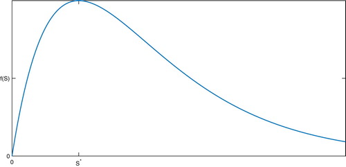
The general desired form of the function f is shown in Figure 1.

Figure 1. Desired shape and behaviour of the function f.

In [27], a function of the form $f\left(S\right)=k_{1}S\exp \left(\right(S^{\ast }-S\left)/S^{\ast }\right)$ was chosen. In this case, if we choose $k_1=k_3{C}^{\ast }/S^{\ast }$, so that $S^{\ast }$ and $C^{\ast }$ are components of the disease-free equilibrium, one can verify that this function satisfies (H1)–(H5). Further, if we note that the disease-free equilibrium value for monocytes is $S^{\ast }=\mu /\alpha$, the condition (H6) reduces to the inequality e>1, and thus imposes no further restrictions on the parameters. In the numerical section of this work, the function f will be of the rational form. However, our approach for much of this article is to analyse the model for any function f which satisfies $\left(H1\right)-\left(H6\right)$.

3. Model equilibria and stability

Upon inspection, it is clear that we have the disease-free equilibrium $E_1=[C^{\ast },S^{\ast },0,0,Z^{\ast }]$, where $C^{\ast }=f\left(S^{\ast }\right)/k_3$, $S^{\ast }=\mu /\alpha$, and $Z^{\ast }=\eta /\delta .$ There is also the equilibrium $E_2=[0,0,0,0,\eta /\delta ]$ which we will refer to as the ‘death equilibrium’ since immune systems are not functional without monocytes. We will first present stability results for these equilibria and then discuss the existence of a third, interior, equilibrium.

The Jacobian of the model is expressed below $J(C,S,I,V,Z)=\left(\begin{array}{ccccc}-k_3& f^{\prime }\left(S\right)+k_{2}aV& 0& k_{2}aS& 0\\ \frac{k_3\mu }{f\left(S^{\ast }\right)}& -\alpha -aV& 0& -aS& 0\\ 0& aV& -\text{β}-\nu Z& aS& -\nu I\\ 0& -aV& k\text{β}& -\gamma -aS& 0\\ 0& 0& \sigma +mZ& 0& mI-\delta \end{array}\right)$ Substituting the disease-free equilibrium into the Jacobian matrix results in $J(C^{\ast },S^{\ast },0,0,Z^{\ast })=\left(\begin{array}{ccccc}-k_3& 0& 0& \frac{a{k}_2\mu }{\alpha }& 0\\ \frac{k_3\mu }{f\left(S^{\ast }\right)}& -\alpha & 0& \frac{-a\mu }{\alpha }& 0\\ 0& 0& -\text{β}-\frac{\nu \eta }{\delta }& \frac{a\mu }{\alpha }& 0\\ 0& 0& k\text{β}& -\gamma -\frac{a\mu }{\alpha }& 0\\ 0& 0& \sigma +\frac{m\eta }{\delta }& 0& -\delta .\end{array}\right)$ The calculation of $det\left[J\right(C^{\ast },S^{\ast },0,0,Z^{\ast })-\lambda I]$ gives the same characteristic polynomial found in [27]: (4) $\begin{array}{rl}p\left(\lambda \right)& =\frac{1}{\alpha \delta }(\lambda +k_3)(\lambda +\alpha )(\lambda +\delta )\left(\alpha \right(\gamma +\lambda \left)\right(\delta (\text{β}+\lambda )+\eta \nu )\\ & +a\mu \left(\delta \right(\text{β}-k\text{β}+\lambda )+\eta \mu ),\end{array}$(4) which yields the following eigenvalues: (5) $\begin{array}{rl}{\lambda }_1& =-\delta \\ {\lambda }_2& =-k_3\\ {\lambda }_3& =-\alpha \\ {\lambda }_4& =\frac{-\mathrm{\Gamma }+\sqrt{{\mathrm{\Gamma }}^2-4\alpha \delta (\alpha \text{β}\gamma \delta -ak\text{β}\delta \mu +a\text{β}\delta \mu +\alpha \gamma \eta \nu +a\eta \mu \nu )}}{2\alpha \delta }\\ {\lambda }_5& =\frac{-\mathrm{\Gamma }-\sqrt{{\mathrm{\Gamma }}^2-4\alpha \delta (\alpha \text{β}\gamma \delta -ak\text{β}\delta \mu +a\text{β}\delta \mu +\alpha \gamma \eta \nu +a\eta \mu \nu )}}{2\alpha \delta }\end{array}$(5) where $\mathrm{\Gamma }=\alpha \text{β}\delta +\alpha \gamma \delta +a\delta \mu +\alpha \eta \nu .$

This gives the same result found in [27], but with a more general model.

Theorem 3.1

If $R_0=\left(ak\text{β}\delta \mu /(\text{β}\delta +\eta \nu )(\alpha \gamma +a\mu )\right)<1,$ then the disease-free equilibrium, $[C^{\ast },S^{\ast },0,0,Z^{\ast }],$ is locally asymptotically stable.

Proof.

Recall that all parameter values are nonnegative. Upon inspection, we can clearly see that all ${\lambda }_i$ aside from ${\lambda }_4$ are either negative or will have real parts that are negative. In order to ensure that ${\lambda }_4$ has a negative real part we must require $\alpha \text{β}\gamma \delta -ak\text{β}\delta \mu +a\text{β}\delta \mu +\alpha \gamma \eta \nu +a\eta \mu \nu >0,$ which leads to the result.

While we have not obtained a global result, our many numerical simulations of the model suggest that the disease-free equilibrium $E_1$ is globally asymptotically stable under the condition $R_0<1$.

By substituting $[C,S,I,V]=[0,0,0,0]$, the model reaches the equilibrium $E_2=[0,0,0,0,\eta /\delta ].$ The resulting Jacobian in this case is: $J(0,0,0,0,\eta /\delta )=\left(\begin{array}{ccccc}-k_3& f^{\prime }\left(0\right)& 0& 0& 0\\ \frac{k_3\mu }{f\left(S^{\ast }\right)}& -\alpha & 0& 0& 0\\ 0& 0& -\text{β}-\frac{\nu \eta }{\delta }& 0& 0\\ 0& 0& k\text{β}& -\gamma -0& 0\\ 0& 0& \sigma +\frac{m\eta }{\delta }& 0& -\delta .\end{array}\right)$ Here the resulting characteristic polynomial is: (6) $\begin{array}{rl}p\left(\lambda \right)& =-\frac{1}{\delta f\left(S^{\ast }\right)}(\gamma +\lambda )(\delta +\lambda )\left(\delta \right(\text{β}+\lambda )+\eta \nu )\\ & (-(k_3+\lambda \left)\right(\alpha +\lambda \left)f\right(S^{\ast })+k_3\mu f^{\prime }(0\left)\right)\end{array}$(6) In this case also we can get expressions for eigenvalues, which are given below: (7) $\begin{array}{rl}{\lambda }_1& =\frac{f\left(S^{\ast }\right)(-k_3-\alpha )-\sqrt{f^2\left(S^{\ast }\right)(k_3^2-2k_3\alpha +{\alpha }^2)+4k_3\mu f^{\prime }\left(0\right)f\left(S^{\ast }\right)}}{2f\left(S^{\ast }\right)}\\ {\lambda }_2& =\frac{f\left(S^{\ast }\right)(-k_3-\alpha )+\sqrt{f^2\left(S^{\ast }\right)(k_3^2-2k_3\alpha +{\alpha }^2)+4k_3\mu f^{\prime }\left(0\right)f\left(S^{\ast }\right)}}{2f\left(S^{\ast }\right)}\\ {\lambda }_3& =-\gamma \\ {\lambda }_4& =-\delta \\ {\lambda }_5& =-\frac{\text{β}\delta +\eta \nu }{\delta }\end{array}$(7) By the assumption that $\mu f^{\prime }\left(0\right)>\alpha f\left(S^{\ast }\right)$, (H6), we see that ${\lambda }_2>0$ for all sets of positive parameters, and thus this equilibrium is always unstable. Formally, this provides us with the following:

Theorem 3.2

Under conditions $\left(H1\right)-\left(H6\right),$ the equilibrium $E_2=[0,0,0,0,\eta /\delta ]$ is unstable for all values of $R_0$.

We were able to establish the following result in the case that $R_0>1$. Since we provide the result with a general function $f\left(S\right)$ that satisfies $\left(H1\right)-\left(H5\right)$, the proof is rather lengthy and somewhat tedious. For this reason, we have included it in Appendix. Numerical simulation of the model suggests that this equilibrium is globally asymptotically stable when it exists.

Theorem 3.3

If $R_0=\left(ak\text{β}\delta \mu /(\text{β}\delta +\eta \nu )(\alpha \gamma +a\mu )\right)>1,$ then there exists a unique interior equilibrium $E_3=[\hat{C},\hat{S},\hat{I},\hat{V},\hat{Z}]$, where $\hat{C}>0,\hat{S}>0,\hat{I}>0,\hat{V}>0,\hat{Z}>0.$

4. Estimation of parameters and comparison to clinical data

From this point on, we will assume that $f\left(S\right)$ has the form (8) $f\left(S\right)=\frac{k_{1}S}{1+{\left(\frac{S}{S^{\ast }}\right)}^2}.$(8) This function is similar to the function used in [1,5,7], which was used to model the production of erythropoietin in response to low red blood cell counts. One difference is that our function satisfies $f\left(0\right)=0$, since M-CSF is a cytokine as opposed to a hormone-like erythropoietin. That is, M-CSF is produced by the monocytes themselves, and so the lack of cells implies a lack of production by those cells. One can also easily verify that condition (H6) reduces to the inequality $1>\frac{1}{2}$ in this case, which imposes no further restrictions on the parameters. In what follows, we will choose values for only those parameters for which we can justify with either biological sources or with values used in other mathematical works. The rest will be estimated from the clinical data obtained in [29]. The half-life of M-CSF has been estimated to be around 7 h [25]. This corresponds to a value of $k_3=-\frac{24}{7}\ln \left(.5\right)\approx 2.38$. The normal range for the concentration of M-CSF is approximately $0.168\pm .61$ international units (IU) per microliter of blood [15]. We choose the mean value of 0.168 for the disease-free equilibrium value, $C^{\ast }$, in our model. The normal range for monocytes in an uninfected individual can be quite large, 200–700 cells per microliter of blood [9,29]. We chose a mid-range value of 440, which corresponds to $S^{\ast }$. If $S^{\ast }$ and $C^{\ast }$ are indeed the disease-free equilibrium values in our model, it is implied that $k_1=2k_3{C}^{\ast }/S^{\ast }\approx 0.0018$. Monocytes can have circulating lifespans of up to 7 days [24]. We assume that on average uninfected cells circulate for 5 days ($1/\alpha$) while infected cells circulate for 4 days ($1/\text{β}$). The primary eliminators of infected monocytes are lymphocytes, in the form of both NK cells and T-cells. Normal counts for these cells can range from 1000–3000 cells per microliter[29]. We choose the mid-range value of 2500 for our disease-free equilibrium value $Z^{\ast }$. The lifespan of these cells can vary greatly, anywhere from a month to a year. Again, we choose a central value of 180 days ($1/\delta$). This implies a value of $\eta =\delta Z^{\ast }\approx 13.89$. In [8], it is stated that the viral clearance rate is up to $2.2{\log }_{10}$ copies per day per millilitre. Considering that our units are per microliter and that the viral units are $\times {10}^6$ copies, this corresponds to a value of $\gamma =1.58\times {10}^{-7}$ in our model.

Also in [8], it is found that the recruitment rate of NK cells was about 0.52 cells per day. Since NK cells make up roughly 12 percent of the total lymphocyte population [23], the value we use is $\sigma =0.0624$. In [9], the viral removal rate is assigned a value of $\nu =0.001$ and the rate at which the immune cells are stimulated by viral contact was assigned the value of m = 0.0005 for several simulations. We will use the same values here. We summarize this discussion with Table 1.

Table 1. Parameter values.

Parameter	Value	Source	Parameter	Value	Source
$S^{\ast }$	440	[9,29]	$Z^{\ast }$	2500	[29]
$C^{\ast }$	0.168	[15]	$k_1$	0.0018	Deduced (see above)
$k_3$	2.38	[25]	α	0.2	[24]
β	0.25	[24]	δ	1/180	[21]
η	13.89	Deduced (see above)	γ	$1.58\times {10}^{-7}$	[8]
σ	0.0624	[8]	ν	0.001	[9]
m	0.0005	[9]

Values for the rest of the parameters in the model are approximated in other works [8,9,21], but vary considerably. This is partly due to the difficulty of measuring parameters such as the infection rate of monocytes by viruses (a) directly. For this reason, we have decided to take an indirect approach such as those presented in [6].

In [29], monocyte counts are given both for patients infected with the DENV2 serotype and for patients infected with the DENV3 serotype, days 2–7 of the infection. The results are quite different, with DENV2 infected patients exhibiting much higher (above the normal range) monocyte counts than the DENV3 infected patients. This suggests that for any given model, parameter values should depend on the particular serotype in question. Since the DENV2 data has a larger variance and would pose more difficulty with the approach of constant monocyte production, we will fit our model to this particular data set and show that the model has the ability to approximate the qualitative behaviour of that data.

Corresponding viral counts are not given in [29]. Some data is available on this [28]. In that work, viral loads were measured in patients infected with the DENV1 serotype. As mentioned in [8], maximal loads can be as high as 5 million copies per microliter. The virus is typically cleared from the body with a week of the onset of symptoms. Since we do not have the viral counts corresponding to the data in [29], we will use a hypothetical data set that agrees with the properties given above.

The data in [29] (page 7, Figure 2(c)) consists of the average daily monocyte counts of two sets of patients, one set with DENV2, and one with DENV3. Table 2 gives the values for the DENV2 group. Since the data is given in the form of a graph, we have used the software WebPlotDigitizer to estimate the data points.

Figure 2. Model results after parameter estimation with several values of w along with DENV2 data.

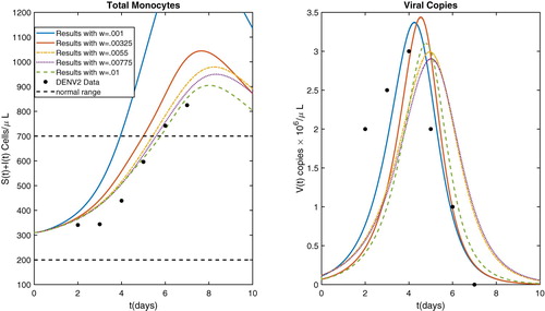
Table 2. Clinical data [29].

Day	DENV2 Monocytes per $\mu L$
2	341
3	344
4	439
5	596
6	742
7	825

To describe the estimation process that we used, we will begin by denoting the monocyte count in [29] on day i of serotype 2 by $s_i$, $i=2,\dots ,7$. We will denote the hypothetical viral count on day i by $v_i$, $i=2,\dots ,7$. Again, we have chosen viral loads in the range of observed data, since they were not reported in [29]. They are given in Table 3.

Table 3. Hypothetical viral loads.

Day	2	3	4	5	6	7
Viral copies $\times {10}^6$	2	2.5	3	2	1	0

In [14], no distinction between infected and uninfected monocytes was made when counts were reported. We will assume that the same is the case in [29]. Our estimation problem will be to minimize the function $\mathfrak{J}:{\mathbb{R}}_{+}^3\to \mathbb{R}$ defined by (9) $\mathfrak{J}(k_2,a,k)=\sum _{i=2}^7{\left(w\left[S\right(i)+I(i)-s_i^j]\right)}^2+\sum _{i=2}^7\left(V\right(i)-v_i{)}^2,$(9) where $S\left(i\right)$, $I\left(i\right)$, and $V\left(i\right)$ are the values of the monocyte, infected monocyte, and viral counts obtained from (3(3) $\begin{array}{rl}\frac{\mathrm{d}C}{\mathrm{d}t}& =f\left(S\right)+k_{2}aSV-k_{3}C\\ \frac{\mathrm{d}S}{\mathrm{d}t}& =\frac{\mu }{C^{\ast }}C-\alpha S-aSV\\ \frac{\mathrm{d}I}{\mathrm{d}t}& =aSV-\text{β}I-\nu IZ\\ \frac{\mathrm{d}V}{\mathrm{d}t}& =k\text{β}I-\gamma V-aSV\\ \frac{\mathrm{d}Z}{\mathrm{d}t}& =\eta +\sigma I+mIZ-\delta Z.\end{array}$(3) ) for the given set of parameter values. We are introducing the weight factor w so that the two sums in (9(9) $\mathfrak{J}(k_2,a,k)=\sum _{i=2}^7{\left(w\left[S\right(i)+I(i)-s_i^j]\right)}^2+\sum _{i=2}^7\left(V\right(i)-v_i{)}^2,$(9) ) are more equally weighted. The parameter estimation was performed for several values of w before we settled on one to continue our analysis. We chose five equally spaced values ranging from w = 0.001 to w = 0.01.

In all of the optimizations, we used the initial condition $\left(C\right(0),S(0),I(0),V(0),Z(0\left)\right)=(.168,300,10,0.1,2000)$. These values were chosen to represent a recently infected individual. That is, the components C, S and Z are chosen in the normal range of an uninfected individual and the initial infected monocyte and viral counts are on the low end of the spectrum observed during dengue infection. This choice is made without knowledge of the actual initial conditions of the patients in the data in [29], since the data was not taken until approximately two days after infection. We then used MATLAB's fminsearch function to minimize $\mathfrak{J}$. The function fminsearch requires an initial guess. After some experimenting, we found that $(k_2,a,k)=[0.005,0.8,15]$ worked well as a starting point for all of the five values of w mentioned above.

The resulting parameter values, along with the resulting value of $R_0$ are given in Table 4 for each of the values of the weight w. The resulting $R_0$ values are all greater than one, which suggests the persistence of the virus. This phenomenon had been established for several viral diseases, including measles and HIV-1. In the case of Dengue, it has been observed that persistent symptoms can be common for two years after infection, even though detectable levels of viral copies are not typically observed after 10–12 days [11]. Further, parameter sets resulting in $R_0>1$ have been used in other mathematical modelling approaches to studying the disease [3,9,21].

Table 4. Parameter values estimated from DENV2 data.

w	$k_2$	a	k	$R_0$
0.001	0.00610	0.98756	13.14848	1.19523
0.00325	0.00541	1.60857	13.02938	1.18440
0.0055	0.00554	0.85299	12.40480	1.12763
0.00775	0.00550	0.85736	12.35033	1.12268
0.01	0.00525	1.62114	12.78318	1.16202

The model output for each of the parameter sets is displayed in Figures 2 and 3. We note here from Figure 2 that the model has the capability to qualitatively fit the data in [29]. That is, the value of total monocytes can exit the normal(uninfected individual)range and then return to normal levels later, even though the uninfected normal equilibrium $S^{\ast }$ was chosen well within the normal range. Using a constant rate of monocyte production, the only way to have model results close to this set of data is to choose the equilibrium value to be the upper extreme of the normal range, which seems unreasonable. Indeed, the models with constant monocyte production the total monocyte count satisfies (2(2) $\begin{array}{rl}\frac{\mathrm{d}}{\mathrm{d}t}\left[S\left(t\right)+I\left(t\right)\right]& =\mu -\alpha S-\text{β}I-\nu IZ\\ & \le \mu -min\{\alpha ,\text{β}\}\left(S\right(t)+I(t\left)\right).\end{array}$(2) ) as mentioned in Section 2. Once the total monocyte count drifts below $S^{\ast }$, it can never attain values above it, and hence never display the behaviour seen in Figure 2.

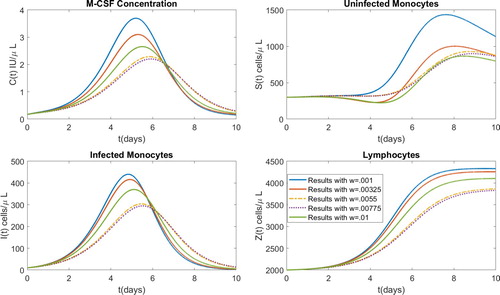
Figure 3. Model results after parameter estimation with several values of w.

In order to finally settle on a set of parameter values, we examined the unweighted $(w=1)$ errors for both the total number of monocytes and the viral copies. The results are presented in Table 5. It becomes clear why the parameter w was introduced when we note that the magnitudes of the errors from the total monocyte counts are much larger than those of the viral copies. Without the parameter w, the optimization would simply ignore the errors resulting from the viral copies. Further, we can see the direct relationship that the viral copy error has with w. That is, larger values of w result in larger errors in the third column of Table 5. The opposite result occurs in the middle column. Based on this, we decided to use the value of w in the middle of the range, w = 0.0055. The parameter values resulting from using w = 0.0055 were used in order to perform the sensitivity analysis that is presented in the following section.

Table 5. Errors obtained from estimations.

w	$\sum _{i=2}^7\left(S\right(i)+I(i)-s_i^j{)}^2$	$\sum _{i=2}^7\left(V\right(i)-v_i{)}^2$
0.001	1.04 $\times {10}^6$	2.35
0.00325	8.8 $\times {10}^4$	4.89
0.0055	2.5 $\times {10}^4$	7.06
0.00775	1.5 $\times {10}^4$	7.46
0.01	1.3 $\times {10}^4$	6.56

5. Sensitivity analysis

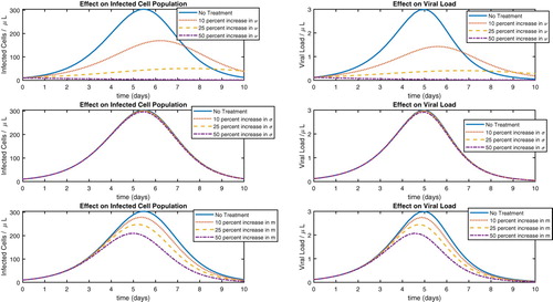
In this section, we will conduct a sensitivity analysis on our model for the parameter set found in the previous section. The motivation is to investigate how effective antiviral or immunostimulatory medications would be, depending on the mechanism by which it works. For example, an antiviral medication might work by simply killing the free viruses. This would correspond to increasing the value of γ. Another approach might be to impede the ability of virus to infect susceptible monocytes in the first place. In the model, this approach could be simulated by reducing the parameter a. A third approach would be to slow down the rate of viral replication in infected monocytes. Reducing the parameter k would simulate a treatment of this type. In the case of immunostimulatory treatments, a medication might increase the rate at which immune cells are able to remove infected monocytes. We will simulate this by increasing ν. Another approach would be to increase the recruitment rates of NK cells or T-Cells. These scenarios can be simulated by increasing σ and m, respectively. Since our motivation is to examine treatment strategies, we will confine our sensitivity analysis to these parameters, which only exist in the model when an infection has occurred.

5.1. Antiviral treaments

To carry out the idea for antiviral treatment, we start with the parameter values resulting from estimation with w = 0.0055 (Table 4) and the parameter values in Table 1. We simulate the model with decreases of a by 10 %, 25 %, and 50 %, and then plot the results along with the value of a found in Table 1. We perform a similar computation with the parameter k, only this time reducing it by 2 %, 5 %, and 10 %. We then proceed with increasing the parameter γ by 100%, 300%, and 700% and plot all of the results, which are shown in Figure 4. The reason for the different degrees by which we are varying the parameters is mathematical. That is, when the model showed less sensitivity to a parameter, we varied that parameter more in an attempt to have plots that were distinguishable.

Figure 4. Sensitivity analysis for antiviral approaches.

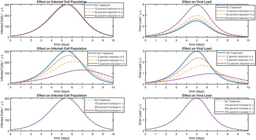
It is clear from Figure 4 that reducing the viral replication rate (k) is the most effective approach. There are medications for other diseases that work in exactly this way. For example, it is known that when quinine was effective in malaria treatment, the mechanism was the reduction of the parasitic replication rate in infected red blood cells. Greatly increasing the rate γ has little effect on the model output, suggesting that increasing the viral death rate is not an effective strategy.

5.2. Immunostimulatory treatments

We now present similar calculations in the case of immunostimulatory treatments. Here as well, we start by plotting the model output resulting from using the values in Table 1 and the values for w = 0.0055 in Table 4. We then perform the simulations with increases in the values of $\nu ,\sigma$ and m by 10 $\mathrm{\%}$, 25 $\mathrm{\%}$, and 50 $\mathrm{\%}$. The results are plotted in Figure 5. Here we see that while increasing the recruitment of T-cells (m) does have some efficacy, increasing the rate of removal of infected monocytes by immune cells (ν) is far more effective. Also, it appears that increasing the recruitment of NK cells would be a very ineffective approach.

Figure 5. Sensitivity analysis for immunostimulatory approaches.

6. Conclusion

In this work, we have generalized a previous model of within-host dengue infection without assuming constant monocyte production [27]. The motivation for the new approach was that observed monocyte counts can be both suppressed [13,29] and elevated [14,29] during infection. Assuming constant monocyte production will typically only display suppressed levels, while our approach has been shown to have the ability to replicate the behaviour of data sets in which some of the monocyte counts are outside of the normal range. We provided local stability results for the general case where the production of M-CSF by monocytes ($f\left(S\right)$) is not specified to an extent beyond satisfying several conditions. For the general case, we have also proven the existence of an interior persistence equilibrium. These general results allow one to experiment with many forms of $f\left(S\right)$ should one particular form seem inadequate. We estimated three model parameters from clinical data [29] and showed that the model has the ability to qualitatively behave in accordance with the data. We also provided a sensitivity analysis by examining many simulations of the model that correspond to antiviral and immunostimulatory treatment approaches. The simulations suggest that antiviral treatments that focus on reducing the viral replication rate are most effective, while immunostimulatory treatments seem most effective if they focus on raising the infected monocyte removal rate by immune cells. Future work in the area will involve theoretically optimizing treatments under the assumption that antiviral medications and immunostimulatory treatments are developed.

Acknowledgments

We would like to enthusiastically thank the reviewers for their careful reading of the original manuscript and whose suggestions greatly improved the final version.

Disclosure statement

No potential conflict of interest was reported by the author(s).

Additional information

Funding

This work was supported by a Fulbright U.S. Scholar grant received by Dr. Jeremy Thibodeaux.

Appendix

Here we will provide a proof of Theorem 3.2. Note that $R_0>1$ implies that k>1, which is important in what follows. Indeed, if $R_0>1$, then we have $ak\text{β}\delta \mu >(\text{β}\delta +\eta \nu )(\alpha \gamma +a\mu )=\text{β}\delta \alpha \gamma +\text{β}\delta a\mu +\eta \nu \alpha \gamma +\eta \nu a\mu >\text{β}\delta a\mu .$ To begin, we define the following parameters (A1) $\begin{array}{rl}{\theta }_1& =a\text{β}\delta (k-1)-a\eta \nu {\tau }_1=\gamma (\text{β}\delta +\eta \nu )\\ {\theta }_2& =a\text{β}m(k-1)+a\sigma \nu {\tau }_2=\gamma (\sigma \nu -\text{β}m)\end{array}$(A1) and provide the following lemmas.

Lemma A.1

If $R_0>1$, then ${\theta }_1\mu -\alpha {\tau }_1>0$, which implies ${\theta }_1>0$.

Proof.

First, an easy computation shows that the condition $R_0>1$ implies ${\theta }_1\mu -\alpha {\tau }_1>0.$ Further, ${\theta }_1>0$ follows readily from $R_0>1.$

Lemma A.2

The inequality $\left({\tau }_1/{\theta }_1\right)>\left(-{\tau }_2/{\theta }_2\right)$ holds for $R_0>1$.

Proof.

First, if ${\tau }_2>0$, we are done since we know that both ${\theta }_1>0$ and ${\tau }_1>0$ if $R_0>0$ and k>1. So let us consider ${\tau }_2<0$. In this case, the inequality above is equivalent to ${\tau }_1{\theta }_2>-{\tau }_2{\theta }_1$. The straightforward, but tedious, calculation of each side of the inequality gives: ${\tau }_1{\theta }_2=-m{\text{β}}^2\delta +mk{\text{β}}^2\delta -m\text{β}\eta \nu +mk\text{β}\eta +\text{β}\delta \nu \sigma +\eta {\nu }^2\sigma$ and $-{\tau }_2{\theta }_1=-m{\text{β}}^2\delta +mk{\text{β}}^2\delta -d\text{β}\eta \nu +\text{β}\delta \nu \sigma -k\text{β}\delta \nu \sigma +\eta {\nu }^2\sigma .$ Upon inspection, we see that ${\tau }_1{\theta }_2>-{\tau }_2{\theta }_1$ reduces to $mk\text{β}\eta \nu >-k\text{β}\delta \nu \sigma$, which demonstrates the result.

Lemma A.3

Assume that $R_0>1.$ Then the first component, $\hat{S}$, of any interior equilibrium $E_3$ of (3(3) $\begin{array}{rl}\frac{\mathrm{d}C}{\mathrm{d}t}& =f\left(S\right)+k_{2}aSV-k_{3}C\\ \frac{\mathrm{d}S}{\mathrm{d}t}& =\frac{\mu }{C^{\ast }}C-\alpha S-aSV\\ \frac{\mathrm{d}I}{\mathrm{d}t}& =aSV-\text{β}I-\nu IZ\\ \frac{\mathrm{d}V}{\mathrm{d}t}& =k\text{β}I-\gamma V-aSV\\ \frac{\mathrm{d}Z}{\mathrm{d}t}& =\eta +\sigma I+mIZ-\delta Z.\end{array}$(3) ) must satisfy $F\left(\hat{S}\right)=0$ with $F\left(S\right)=\frac{f\left(S\right)}{S}-\frac{f\left(S^{\ast }\right)}{S^{\ast }}+\frac{ak\text{β}(k_2-\frac{f\left(S^{\ast }\right)}{\mu })}{aS+\gamma }G\left(S\right),$ and ${\displaystyle G\left(S\right)=\left({\theta }_{1}S-{\tau }_1\right)/({\theta }_{2}S+{\tau }_2)}$. The values of $\hat{C},\hat{I},\hat{V}$ and $\hat{Z}$, are given by (A2) $\hat{Z}=\frac{\eta +\sigma \hat{I}}{\delta -m\hat{I}},\hat{V}=\frac{k\text{β}\hat{I}}{\gamma +a\hat{S}},\hat{C}=\frac{k_1}{\alpha k_3}(a\hat{S}\hat{V}+\alpha \hat{S}),\hat{I}=G\left(\hat{S}\right)$(A2)

Proof.

An equilibrium point of (3(3) $\begin{array}{rl}\frac{\mathrm{d}C}{\mathrm{d}t}& =f\left(S\right)+k_{2}aSV-k_{3}C\\ \frac{\mathrm{d}S}{\mathrm{d}t}& =\frac{\mu }{C^{\ast }}C-\alpha S-aSV\\ \frac{\mathrm{d}I}{\mathrm{d}t}& =aSV-\text{β}I-\nu IZ\\ \frac{\mathrm{d}V}{\mathrm{d}t}& =k\text{β}I-\gamma V-aSV\\ \frac{\mathrm{d}Z}{\mathrm{d}t}& =\eta +\sigma I+mIZ-\delta Z.\end{array}$(3) ) satisfies the nonlinear system (A3) $\begin{array}{rl}f\left(S\right)+k_{2}aSV-k_{3}C& =0\\ \frac{\mu }{C^{\ast }}C-\alpha S-aSV& =0\\ aSV-\text{β}I-\nu IZ& =0\\ \text{β}kI-\gamma V-aSV& =0\\ \eta +\sigma I+mIZ-\delta Z& =0,\end{array}$(A3) where, again,    $C^{\ast }=f\left(S^{\ast }\right)/k_3$ and $S^{\ast }=\mu /\alpha .$

From the fourth and fifth equations in (A3(A3) $\begin{array}{rl}f\left(S\right)+k_{2}aSV-k_{3}C& =0\\ \frac{\mu }{C^{\ast }}C-\alpha S-aSV& =0\\ aSV-\text{β}I-\nu IZ& =0\\ \text{β}kI-\gamma V-aSV& =0\\ \eta +\sigma I+mIZ-\delta Z& =0,\end{array}$(A3) ) we obtain (A4) $Z=\frac{\eta +\sigma I}{\delta -mI},V=\frac{\text{β}kI}{aS+\gamma }.$(A4) Moreover, the third and fourth equations give the equality $(\text{β}+\nu Z)I=\text{β}kI-\gamma V,$ and hence (A5) $I\left(\text{β}(k-1)+\frac{\nu (\eta +\sigma I)}{\delta -mI}+\frac{\text{β}k\gamma }{aS+\gamma }\right)=0$(A5) If I = 0 we obtain the equilibrium points $E_1$ and $E_2$. Now, if $I\ne 0$ we deduce from (A5(A5) $I\left(\text{β}(k-1)+\frac{\nu (\eta +\sigma I)}{\delta -mI}+\frac{\text{β}k\gamma }{aS+\gamma }\right)=0$(A5) ) that $I=\frac{{\theta }_{1}S-{\tau }_1}{{\theta }_{2}S+{\tau }_2}.$ Substituting the above equation in the last equation of (A4(A4) $Z=\frac{\eta +\sigma I}{\delta -mI},V=\frac{\text{β}kI}{aS+\gamma }.$(A4) ) we have $V=\frac{\text{β}k({\theta }_{1}S-{\tau }_1)}{(aS+\gamma )({\theta }_{2}S+{\tau }_2)}.$ Finally, by the first and second equations in (A3(A3) $\begin{array}{rl}f\left(S\right)+k_{2}aSV-k_{3}C& =0\\ \frac{\mu }{C^{\ast }}C-\alpha S-aSV& =0\\ aSV-\text{β}I-\nu IZ& =0\\ \text{β}kI-\gamma V-aSV& =0\\ \eta +\sigma I+mIZ-\delta Z& =0,\end{array}$(A3) ) we obtain (A6) $S\left(\frac{f\left(S\right)}{S}-\frac{k_3{C}^{\ast }\alpha }{\mu }+\frac{(k_2-\frac{k_3{C}^{\ast }}{\alpha })ak\text{β}({\theta }_{1}S-{\tau }_1)}{(aS+\gamma )({\theta }_{2}S+{\tau }_2)}\right)=0$(A6) Again, we do not want solutions with S = 0 and so the first component of any interior equilibrium satisfies the equation $F\left(S\right)=0$ where $F\left(S\right)=\frac{f\left(S\right)}{S}-\frac{f\left(S^{\ast }\right)}{S^{\ast }}+\frac{(k_2-\frac{f\left(S^{\ast }\right)}{\mu })ak\text{β}({\theta }_{1}S-{\tau }_1)}{(aS+\gamma )({\theta }_{2}S+{\tau }_2)}.$

The following lemma provides a positive solution of $F\left(S\right)=0.$

Lemma A.4

Suppose that $R_0>1$. Let $F\left(S\right)=f\left(S\right)/S-f\left(S^{\ast }\right)/S^{\ast }+(k_2-f\left(S^{\ast }\right)/\mu )ak\text{β}({\theta }_{1}S-{\tau }_1)/(aS+\gamma )({\theta }_{2}S+{\tau }_2)$. Then there is one unique solution of $F\left(S\right)=0$ in the interval $({\tau }_1/{\theta }_1,\mathrm{\infty })$.

Proof.

Notice that $F\left({\tau }_1/{\theta }_1\right)=\left({\theta }_1/{\tau }_1\right)f\left({\tau }_1/{\theta }_1\right)-\left(\alpha /\mu \right)f\left(\mu /\alpha \right)>0$ from Lemma 1 and from the assumption that $f\left(S\right)/S$ is strictly decreasing (H5). Further, it can be seen that $\underset{S\to \mathrm{\infty }}{lim}F\left(S\right)=-f\left(S^{\ast }\right)/S^{\ast }$. So we can find an $\tilde{S}>0$ such that $F\left(\tilde{S}\right)<0.$ So by the Intermediate Value Theorem, there exists at least one solution of $F\left(S\right)=0$ in $({\tau }_1/{\theta }_1,\tilde{S}).$ To show that this solution is unique, we will consider $F\left(S\right)=H\left(S\right)+Q\left(S\right)$, where $H\left(S\right)=f\left(S\right)/S-f\left(S^{\ast }\right)/S^{\ast }$ and $Q\left(S\right)=(k_2-f\left(S^{\ast }\right)/\mu )ak\text{β}({\theta }_{1}S-{\tau }_1)/(aS+\gamma )({\theta }_{2}S+{\tau }_2)$. Let us first consider the case $k_2-f\left(S^{\ast }\right)/\mu >0$. We can easily see that $H\left(S\right)$ is a strictly decreasing function on $({\tau }_1/{\theta }_1,\mathrm{\infty })$, being nonnegative for $S\le S^{\ast }$ and negative for $S>S^{\ast }.$ Further, it has the same horizontal asymptote as $F\left(S\right).$ Now, if $Q\left(S\right)$ has a vertical asymptote (i.e. ${\tau }_2<0$), Lemma A.2 implies that it cannot occur in $({\tau }_1/{\theta }_1,\mathrm{\infty }).$ Given this, we can see that $-Q\left(S\right)\le 0$, for all $S\ge {\tau }_1/{\theta }_1$. So any intersection of $H\left(S\right)$ and $-Q\left(S\right)$ must occur in $(S^{\ast },\mathrm{\infty })$. Upon calculating $-Q^{\prime }\left(S\right)$, we find $-Q^{\prime }\left(S\right)=\left(k_2-\frac{f\left(S^{\ast }\right)}{\mu }\right)ak\text{β}\frac{q\left(S\right)}{(aS+\gamma {)}^2({\theta }_{2}S+{\tau }_2{)}^2},$ where $q\left(S\right)$ is the quadratic function given by $q\left(S\right)=a{S}^2{\theta }_1{\theta }_2-2aS{\theta }_2{\tau }_1-\gamma {\theta }_2{\tau }_1-\gamma {\theta }_1{\tau }_2-a{\tau }_1{\tau }_2.$ The vertex of this parabola will occur at $S={\tau }_1/{\theta }_1$ and with help from Lemma A.3 it can be confirmed that $q\left({\tau }_1/{\theta }_1\right)<0$. Hence this quadratic will have exactly one positive root in $({\tau }_1/{\theta }_1,\mathrm{\infty })$, say $x^{\ast }$. Therefore the function $-Q\left(S\right)$ will decrease on the interval $(0,x^{\ast })$ and increase on $(x^{\ast },\mathrm{\infty })$, and will satisfy $\underset{S\to \mathrm{\infty }}{lim}[-Q(S\left)\right]=0.$ This only leaves the possibility for one intersection of $H\left(S\right)$ and $-Q\left(S\right)$ in $({\tau }_1/{\theta }_1,\mathrm{\infty })$, or more specifically in $(\mu /\alpha ,\mathrm{\infty })$, and concludes the proof for $k_2-\left(f\left(S^{\ast }\right)/\mu \right)>0$. The proof for the case $k_2-\left(f\left(S^{\ast }\right)/\mu \right)<0$ is similar and yields a solution in $({\tau }_1/{\theta }_1,S^{\ast })$.

Lemma A.5

The unique solution $S=\hat{S}$ obtained in Lemma (A.4) generates a unique interior equilibrium $E_3$ in ${\mathbb{R}}_{+}^5$.

Proof.

First, we will demonstrate that the unique solution $\hat{S}\in ({\tau }_1/{\theta }_1,\mathrm{\infty })$ of $F\left(S\right)=0$ does indeed provide an equilibrium $E_3$ in ${\mathbb{R}}_{+}^5$. It suffices to show that this choice of S produces positive values in (A2(A2) $\hat{Z}=\frac{\eta +\sigma \hat{I}}{\delta -m\hat{I}},\hat{V}=\frac{k\text{β}\hat{I}}{\gamma +a\hat{S}},\hat{C}=\frac{k_1}{\alpha k_3}(a\hat{S}\hat{V}+\alpha \hat{S}),\hat{I}=G\left(\hat{S}\right)$(A2) ). Clearly, $\hat{I}=G\left(\hat{S}\right)>0.$ Note that $G\left({\tau }_1/{\theta }_1\right)=0$ and $\frac{dG}{dS}=\frac{{\tau }_2{\theta }_1+{\tau }_1{\theta }_2}{({\theta }_{2}S+{\tau }_2{)}^2}>0$ if $S\ne -{\tau }_2/{\theta }_2$. So $G\left(S\right)$ is strictly increasing and is bounded above by ${\theta }_1/{\theta }_2$ on $({\tau }_1/{\theta }_1,\mathrm{\infty })$. This implies that $\hat{I}=G\left(\hat{S}\right)=\frac{{\theta }_1\hat{S}-{\tau }_1}{{\theta }_2\hat{S}+{\tau }_2}<\frac{{\theta }_1}{{\theta }_2}=\frac{a\text{β}\delta (k-1)-a\eta \nu }{a\text{β}m(k-1)+a\sigma \nu }<\frac{a\text{β}\delta (k-1)}{a\text{β}m(k-1)}=\frac{\delta }{m}$ on $({\tau }_1/{\theta }_1,\mathrm{\infty })$. Therefore, $\hat{I}<\delta /m$ and thus $\hat{Z}=\left(\eta +\sigma \hat{I}\right)/\left(\delta -m\hat{I}\right)>0$. This value of $\hat{I}$ also clearly produces positive values for $\hat{C}$ and $\hat{V}$.

Now we will argue that if a solution $\hat{S}$ of $F\left(S\right)=0$ exists outside of $({\tau }_1/{\theta }_1,\mathrm{\infty })$, then it will result in a equilibrium outside of ${\mathbb{R}}_{+}^5.$ If the function F from Lemma (A.4) has no vertical asymptote (i.e. ${\tau }_2>0$), then it is clear that for any value $0<\hat{S}<{\tau }_1/{\theta }_1,$ we will have $\hat{I}=\left({\theta }_1\hat{S}-{\tau }_1\right)/\left({\theta }_2\hat{S}+{\tau }_2\right)<0.$ So it remains to examine the case ${\tau }_2<0$. Recall that by Lemma A.2 we have $-{\tau }_2/{\theta }_2<{\tau }_1/{\theta }_1.$ Further, if $-{\tau }_2/{\theta }_2<\hat{S}<{\tau }_1/{\theta }_1$, then $\hat{I}<0$ and thus of no interest biologically. Finally, assume that there is a solution $\hat{S}$ of $F\left(S\right)=0$ that satisfies $0<\hat{S}<-{\tau }_2/{\theta }_2$. Again, $G^{\prime }\left(S\right)>0$ if $S\ne -{\tau }_2/{\theta }_2$. So $G\left(S\right)$ is bounded below by $-{\tau }_1/{\tau }_2$ on $0<S<-{\tau }_2/{\theta }_2$. That is $I>-{\tau }_1/{\tau }_2$ if $0<S<-{\tau }_2/{\theta }_2$. From this, we see that $\hat{I}>\frac{-{\tau }_1}{{\tau }_2}=\frac{\gamma (\text{β}\delta +\nu \eta )}{-\gamma (\sigma \nu -\text{β}m)}=\frac{\text{β}\delta +\eta \nu }{\text{β}m-\sigma \nu }>\frac{\text{β}\delta }{\text{β}m}=\frac{\delta }{m},$ which implies that $\hat{Z}<0$.

From these results, we see that there exists one unique solution of $F\left(S\right)=0$ in $({\tau }_1/{\theta }_1,\mathrm{\infty })$ that generates a unique equilibrium $E_3$ in ${\mathbb{R}}_{+}^5.$

Numerical simulation of the model suggests that this equilibrium is globally asymptotically stable when it exists.

References

- A.S. Ackleh, K. Deng, K. Ito, and J.J. Thibodeaux, A structured erythropoiesis model with nonlinear cell maturation velocity and hormone decay rate, Math. Biosci. 204 (2006), pp. 21–48. doi: 10.1016/j.mbs.2006.08.004
- M. Akashi and H.P. Koeffler, Colony stimulating factors: Regulation of production, in Modern Trends in Human Leukemia IX. Haematology and Blood Transfusion/Hämatologie und Bluttransfusion, R. Neth, E. Frolova, R. C. Gallo, M. F. Greaves, B. V. Afanasiev and E. Elstner, eds., Springer, Berlin, 1992, pp. 83–92.
- H. Ansari and M. Hesaraaki, A with-In host dengue infection model with immune response and beddington-DeAngelis incidence rate, Appl. Math. 3 (2012), pp. 177–184. doi: 10.4236/am.2012.32028
- A.T. Bäck and Å. Lundkvist, Dengue viruses – an overview, Infect. Ecol. Epidemiol. 3 (2013), p. 3. doi:10.3402/iee:v3i0.19839.
- H.T. Banks, C.T. Cole, P.M. Schlosser, and H.T. Tran, Modeling and optimal regulation of erythropoiesis subject to benzene intoxication, Math. Biosci. Eng. 1 (2004), pp. 15–48. doi: 10.3934/mbe.2004.1.15
- H.T. Banks, K. Kunisch, Estimation Techniques for Distributed Parameter Systems, Birkhauser, Boston, MA, 1989.
- J. Bélair, M.C. Mackey, and J.M. Mahaffy, Age-structured and two-delay models for erythropoiesis, Math. Biosci. 128 (1995), pp. 317–346. doi: 10.1016/0025-5564(94)00078-E
- R. Ben-Shachar and K. Koelle, Minimal within-host dengue models highlight the specific roles of the immune response in primary and secondary dengue infections, J. R. Soc. Interface 12 (2015), pp. 20140886. doi: 10.1098/rsif.2014.0886
- H.E. Clapham, V. Tricou, N.V.V Chau, C.P. Simmons, and N.M. Ferguson, Within-host viral dynamics of dengue serotype 1 infection, J. R. Soc. Interface 11 (2014), pp. 20140094. doi: 10.1098/rsif.2014.0094
- Farlex and Partners Medical Dictionary, 2009.
- G. García, N. González, A.B. Pérez, B. Sierra, E. Aguirre, D. Rizo, A. Izquierdo, L.Sánchez, D. Díaz, M. Lezcay, B. Pacheco, K. Hirayama, and M.G. Guzmán, Long-term persistence of clinical symptoms in dengue-infected persons and its association with immunological disorders, Int. J. Infect. Dis. 15 (2011), pp. e38–e43. doi: 10.1016/j.ijid.2010.09.008
- T.P. Gujarati and G.J. Ambika, Virus antibody dynamics in primary and secondary dengue infections, Math. Biol. 69 (2014), pp. 1773–1800. doi: 10.1007/s00285-013-0749-4
- S. Kalayanarooj, D.W. Vaughn, S. Nimmannitya, S. Green, S. Suntayakorn, N. Kunentrasai, W.Viramitrachai, E. Ratanachu-eke, S. Kiatpolpoj, B.L. Innis, A.L. Rothman, A. Nisalak, and F.A. Ennis, Early clinical and laboratory indicators of acute dengue illness, J. Infect. Dis. 176 (1997), pp. 313–321. doi: 10.1086/514047
- B.G. Klekamp, Assessing the relationship of monocytes with primary and secondary dengue infection among hospitalized dengue patients in Malaysia, 2010: A cross-sectional study, Graduate theses and dissertations, 2011. http://scholarcommons.usf.edu/etd/3185.
- Y. Le Meur, V. Leprivey-Lorgeot, S. Mons, M. José, J. Dantal, B. Lemauff, J.C. Aldigier, C.Leroux-Robert, and V. Praloran, Serum levels of macrophage-colony stimulating factor (M-CSF): a marker of kidney allograft rejection, Nephrol. Dial. Transpl. 19 (2004), pp. 1862–1865. doi: 10.1093/ndt/gfh257
- A. Mishra, A within-host model of dengue viral infection dynamics, Applied Analysis in Biological and Physical Sciences, Springer Proceedings in Mathematics and Statistics, 2016. doi:10.1007/978-81-322-3640-59.
- R. Nikin-Beers and S.M. Ciupe, The role of antibody in enhancing dengue virus infection, Math. Biosci. 263 (2015), pp. 83–92. doi: 10.1016/j.mbs.2015.02.004
- R. Nikin-Beers, J.C. Blackwood, L.M. Childs, and S.M. Ciupe, Unraveling within-host signatures of dengue infection at the population level, J. Theoretical Biol. 446 (2018), pp. 79–86. doi: 10.1016/j.jtbi.2018.03.004
- R. Nikin-Beers and S.M. Ciupe, Modelling original antigenic sin in dengue viral infection, Math. Med. Biol. 35 (2018), pp. 257–272. doi: 10.1093/imammb/dqx002
- S. Noisakran, K. Chokephaibulkit, P. Songprakhon, N. Onlamoon, H.M. Hsiao, F. Villinger, A. Ansari, and G.C. Perng, A reevaluation of the mechanisms leading to dengue hemorrhagic fever, Ann. N Y Acad. Sci. 1171(Suppl 1) (2009), pp. E24–E35. doi: 10.1111/j.1749-6632.2009.05050.x
- N. Nuraini, H. Tasman, E. Soewono, and K.A. Sidarto, A with-in host dengue infection model with immune response, Math. Comput. Model 49 (2009), pp. 1148–1155. doi: 10.1016/j.mcm.2008.06.016
- T. Pang, M.J. Cardosa, and G.M.G. Guzman, Of cascades and perfect storms: the immunopathogenesis of dengue haemorrhagic fever-dengue shock syndrome (DHF/DSS), Immunol. Cell Biol. 85 (2007), pp. 43–45. doi: 10.1038/sj.icb.7100008
- V. Pascal, N. Schleinitz, C. Brunet, S. Ravet, E. Bonnet, X. Lafarge, M. Touinssi, D. Reviron, J.F.Viallard, J.F. Moreau, J. Déchanet-Merville, P. Blanco, J.R. Harlé, J. Sampol, E. Vivier, F. Dignat-George, and P. Paul, Comparative analysis of NK cell subset distribution in normal and lymphoproliferative disease of granular lymphocyte conditions, Eur. J. Immunol. 34 (2004), pp. 2930–2940. doi: 10.1002/eji.200425146
- A.A. Patel, Y. Zhang, J.F. Fullerton, The fate and lifespan of human monocyte subsets in steady state and systemic inflammation. J. Exp. Med. 214 (2017), pp. 1913–1923. doi: 10.1084/jem.20170355
- P. Roth, M.G. Dominguez, and E.R. Stanley, The effects of colony-stimulating factor-1 on the distribution of mononuclear phagocytes in the developing osteopetrotic mouse, Blood 91 (1998), pp. 3773–3783. doi: 10.1182/blood.V91.10.3773
- P. Sun, K. Bauza, S. Pal, Z. Liang, S.J. Wu, C. Beckett, T. Burgess, K. Porter, Infection and activation of human peripheral blood monocytes by dengue viruses through the mechanism of antibody-dependent enhancement, Virology 421 (2011), pp. 245–252. doi: 10.1016/j.virol.2011.08.026
- J.J. Thibodeaux and M. Hennessey, A within-Host model of dengue infection with a non-constant monocyte production rate, Appl. Math. 7 (2016), pp. 2382–2393. doi: 10.4236/am.2016.718187
- V. Tricou, N.N. Minh, J. Farrar, H.T. Tran, and C.P. Simmons, Kinetics of viremia and NS1 antigenemia are shaped by immune status and virus serotype in adults with dengue, PLoS Negl. Trop. Dis. 5 (2011), pp. e1309. doi:10.1371/journal.pntd.0001309.
- J.J. Tsai, J.S. Chang, K. Chang, P.C. Chen, L.T. Liu, T.C. Ho, S.S. Tan, Y.W. Chien, Y.C. Lo, and G.C. Perng, Transient monocytosis subjugates low platelet count in adult dengue patients, Biomed. Hub 2 (2017), pp. 457785. doi:10.1159/000457785.
- W.K. Wang, T.L. Sung, Y.C. Tsai, C.L. Kao, S.M. Chang, and C.C. King, Detection of dengue virus replication in peripheral blood mononuclear cells from dengue virus type 2-infected patients by a reverse transcription-real-time PCR assay, J. Clin. Microbiol. 40 (2002), pp. 4472–4478. doi: 10.1128/JCM.40.12.4472-4478.2002
- World Health Organization, Tropical Disease Research, Making Health Research Work for Poor People, Progress 2003–2004, Geneva, 2005.