Stochastic control of single-species population dynamics model subject to jump ambiguity

Abstract

A logistic type stochastic control model for cost-effective single-species population management subject to an ambiguous jump intensity is presented based on the modern multiplier-robust formulation. The Hamilton-Jacobi-Bellman-Isaacs (HJBI) equation for finding the optimal control is then derived. Mathematical analysis of the HJBI equation from the viewpoint of viscosity solutions is carried out with an emphasis on the non-linear and non-local term, which is a key term arising due to the jump ambiguity. We show that this term can be efficiently handled in the framework of viscosity solutions by utilizing its monotonicity property. A numerical scheme to discretize the HJBI equation is presented as well. Our model is finally applied to management of algae population in river environment. Optimal management policies ranging from the short-term to long-term viewpoints are numerically investigated.

KEYWORDS:

• Population dynamics
• jump ambiguity
• Hamilton-Jacobi-Bellman-Isaacs equation
• non-linearity and non-locality
• algae bloom

2010 Mathematics Subject Classifications:

• 34B10
• 35D40
• 65M06
• 92D25
• 93E20

1. Introduction

Management of biological population, such as biological resources and invasive species, is a ubiquitous problem in research areas of biology, ecology, and environment [61]. Examples are sustainable fishery resources harvesting [22], timber harvesting [31], and population control of invasive insects [66]. From a theoretical standpoint, such population dynamics can be reasonably considered as stochastic processes because of inherently nonlinear and complicated background biological processes [43]. Continuous-time [4, 45], discrete-time [1, 21], and hybrid [68, 69] stochastic process modelling methodologies have been successfully applied to biological population dynamics.

The dynamic programming principle is a central mathematical principle in biological population management considering the stochasticity [62] owing to its flexibility that can handle a wide variety of system dynamics. One of the most successful applications of the dynamic programming principle is stochastic control problems where the system dynamics follow stochastic differential equations (SDEs) [28, 58]. SDEs have been fundamental tools for describing population dynamics. Recent application examples of the stochastic control with SDEs to biological population management include early observation of extinctions in a model ecosystem [63], disease dynamics control spread in host trees [39], sustainable management of a fish-eating bird as a predator of inland fishery resources [70], and algae bloom control in a dam-downstream reach [75].

In practice, decision-making models in biological population management often face with model uncertainty, or model ambiguity, in addition to the inherent stochasticity of the population dynamics. The model parameters, such as the population growth rate and its intensity, are often difficult to accurately estimate (bird population management in Lebreton and Clobert [44], eutrophication analysis in Borsuk et al. [13], fisheries management in Collie et al. [23]). We therefore usually cannot disregard model ambiguity. Models to efficiently describe the ambiguity based on interval-valued parameters have been analyzed in ecological and environmental research areas [26, 80]. Quantifying and handling model ambiguities are central topics of decision-making in ecological planning [84]. Mathematical programming methodology to deal with uncertain population dynamics has recently been developed focusing on invasive species management [37]. Problems of environmental economics, which also involve evaluation of biological and socio-economic dynamics, are also subject to inherent uncertainties [34]. Ambiguity of system dynamics is thus ubiquitous in many research areas related to environmental, ecological, and biological problems. Models considering ambiguities would potentially serve as a robust mathematical tool for the decision-makings in the population management.

One of the most successful approaches to handle stochastic system dynamics subject to model ambiguity is the multiplier-robust control [32]. This approach is based on the concept of stochastic control, in which model ambiguity is represented by nature as an opposite player of the decision-maker. The ambiguity is introduced through the method of measure change by a Girsanov’s transformation [32, 38]. In the framework of multiplier-robust control, the control problem subject to ambiguity becomes a stochastic differential game in which a penalization term is added to the original performance index to be optimized. This penalty term is formulated based on a relative entropy measuring the distance between the nominal and ambiguous models [32]. One advantageous point of the multiplier-robust control is that solving a stochastic control problem subject to ambiguity can be reduced to finding an appropriate solution to a Hamilton-Jacobi-Bellman-Isaacs (HJBI) equation: a concrete mathematical object, which is a degenerate nonlinear (integro-) differential equation [32, 83]. The multiplier-robust control has long been used in economics, especially finance [2], insurance [83, 85], commodity [19], and bank management [15]. Its application to environmental [50] and ecological problems [76] have also been carried out very recently. Analysis of the HJBI equations, whose forms are problem-dependent, have been carried out in an analytical manner [35, 46] or in an abstract manner from the viewpoint of viscosity solutions [11, 25]: an appropriate solution concept for differential equations including HJBI equations [24].

In biological population management, the dynamics to be controlled is often subject to jump disturbances. Such jumps represent catastrophic events that stochastically occur like epidemics, floods, and hurricanes [7]. These disturbances are described with a Poisson process in the simplest case, and with a Lévy process in a more complicated case [58]. Several theoretical models give similar predictions that the jump intensity is a critical factor in analyzing population extinction problems from a long-term viewpoint [47, 48, 60]. However, because jump disturbances are not time-continuously observable, quantifying their behaviour, such as their magnitude and occurring intensity, would not be an easy task in practice. This problem can be effectively addressed with the help of the multiplier-robust control, with which decision-makings in population management can be achieved in a more robust manner against ambiguity. To our knowledge, such an approach has not been thoroughly addressed. This is a non-trivial problem, but maybe highly technical. This is the motivation of this paper.

The main objective of this paper is to newly formulate a stochastic control problem of cost-effective biological population management subject to a jump ambiguity. There exist at least two differences between the present and previous models of the authors [71, 72]. Firstly, the model in [71] does not consider the model ambiguity. Therefore, the presented and the previous models [71] are completely different. Secondly, the model in [72] only considers the ambiguity of decaying population dynamics, and thus does not consider the population growth. The population dynamics to be controlled is based on a single-species logistic type SDE [49, 71] as a nominal model. We assume that the jump distribution is known while the jump intensity is ambiguous for the sake of simplicity of analysis. The present problem is formulated in an infinite horizon, and the resulting HJBI equation is an integro-differential equation having a term that is non-linear and non-local. This term arises due to the jump ambiguity, and potentially becomes a difficulty in both mathematical and numerical analyses of the model. However, the term possesses a certain monotone property, which serves as a devise to overcome this difficulty [72]. With this in mind, from the viewpoint of viscosity solutions [6, 24], we prove that the HJBI equation admits a unique continuous viscosity solution: the value function. In addition, we show that a simple finite difference scheme can discretize the HJBI equation. We also show its convergence property in a viscosity sense. Finally, we present a numerical application example of the present model to algae bloom management in a dam-downstream reach. Optimal management policies ranging from the short-term to long-term, ergodic viewpoints are then investigated. We find that the algae growth is suppressed by the jump disturbances for short-term management, while by human interventions for long-term management. This paper thus contributes to new biological population management modelling, its mathematical and numerical analyses, and an application.

The rest of this paper is organized as follows. Section 2 presents the mathematical model and derives the HJBI equation. Differences among the present and previous models are discussed here as well. Section 3 presents mathematical analysis results of the equation. Section 4 focuses on numerical investigation of the algae bloom management. Section 5 concludes this paper and presents our future perspectives. Appendix A contains the proofs of lemmas and propositions stated in the main text.

We assume a dynamic programming principle for the zero-sum differential game throughout this paper as in the several previous works [83, 85]. This is a non-trivial problem, but maybe highly technical.

2. Mathematical model

2.1. Problem setting

We consider continuous-time temporal evolution of single-species population dynamics in a habitat. Modelling and analysis in this paper are under the conventional setting of optimal control of jump-diffusion processes [58]. The decision-maker of the present optimization problem is the manager of the population or its habitat, such as a local government of the region including the habitat.

The standard Brownian motion defined on the usual complete probability space is denoted as $B_t$ at time $t$. The standard compound Poisson process defined on the complete probability space is denoted as $P_t$ at time $t$. Its jump intensity, which is the inverse of the mean time interval between each successive jumps, is denoted as $\lambda >0$. The jump size $z$ at each jump follows the probability distribution $g=g\left(z\right)$ having the compact support $Z$ in $\left(0,1\right)$. Trivially, ${\int }_{Z}g\left(z\right)\text{d}z=1$. We assume that $B_t$ and $P_t$ are independent with each other. The natural filtration generated by $B_t$ and $P_t$ are denoted as ${\mathcal{F}}_t$. Set $\mathcal{F}=\{{\mathcal{F}}_t{\}}_{t\ge 0}$. The population in the habitat is denoted as $X_t$ at time $t$, which is a continuous-time stochastic process adapted to ${\mathcal{F}}_t$. We assume that $X_t$ ($t\ge 0$) is non-negative and càdlàg. The $k$th jump time is denoted as ${\tau }_k$ ($k=1,2,3,\dots$) with ${\tau }_0=0$. The jump intensity at ${\tau }_k$ is denoted $z_k$ as with $z_0=0$. The control variable to represent harvesting of the population at time $t$ is denoted as $q_t$, which is a continuous-time variable adapted to ${\mathcal{F}}_t$ and has the compact range $Q=\left[q_{min},q_{max}\right]$ with $0<q_{min}<q_{max}<+\mathrm{\infty }$. The environmental capacity is a biological parameter that determines the maximum amount of the population in the habitat. The environmental capacity here may depend on the control $q$ [71] such that $K:Q\to \left[K_{min},K_{max}\right]$ with positive constants $0<K_{min}<K_{max}<+\mathrm{\infty }$. We assume that $K$ is Lipschitz continuous and increasing in $Q$. Set $\mathrm{\Omega }=\left[0,K_{max}\right]$ and $\hat{\mathrm{\Omega }}=\left(0,K_{max}\right]$. The set of controls $q_t$ ($t\ge 0$) valued in $Q$, measurable, and adapted to ${\mathcal{F}}_t$ is denoted as $\mathcal{Q}$.

2.2. SDE without ambiguity

The Itô’s SDE describing the population dynamics without model ambiguity is set as (1) $\text{d}{X}_t=X_t\left(1-\frac{X_t}{K\left(q_t\right)}\right)\left(r\left(X_t\right)\text{d}t+\sigma {\chi }_{\left\{X_t\le K\left(q_t\right)\right\}}\text{d}{B}_t\right)-\alpha \left(q_t\right)X_t\text{d}t-X_{t-}\text{d}{P}_t,t>0$(1) subject to an initial condition $X_0=x\in \mathrm{\Omega }$. Here, $X_{t-}=\underset{s\to t-0}{lim}{X}_s$, $r>0$ is the intrinsic growth rate such that the function $xr\left(x\right)$ is Lipschitz continuous with respect to $x\in \mathrm{\Omega }$, $\alpha \ge 0$ is the harvesting rate that is Lipschitz continuous and positive in $Q$, and $\sigma >0$ is a constant volatility modulating continuous stochastic disturbance involved in the population dynamics. The indicator function for a set $S$ is denoted as ${\chi }_S$. At each jump time ${\tau }_k$, the population changes as $X_{{\tau }_k}=\left(1-z_k\right)X_{{\tau }_k-}$ by the last term of (1).

The SDE (1) is a generalization of the logistic models [49, 71], and has both continuous and jump stochastic noises. Its left-hand side represents temporal variation of the population. In the right-hand side, the first term represents the continuous controlled logistic growth, the second term represents the continuous decrease of the population by the harvesting, and the third term represents the catastrophic decrease of the population. In the context of algae bloom management in a dam-downstream river environment that we focus on later, the control variable $q$ is the controllable river flow (flow discharge or flow velocity) by a dam, and the jump disturbance corresponds to floods which on the other hand are assumed to be not controllable and catastrophic. The continuous disturbance is reasonably considered due to flow variability as discussed in Ceola et al. [20]. The algae population is gradually flushed out by the flow [20, 65, 75, 76] and this effect is modelled by the second term in (1).

2.3. SDE with ambiguity

An ambiguous counterpart of the SDE (1) is formulated. The ambiguity in this paper is the model uncertainty that the decision-maker evaluates. The amount of ambiguity depends on his/her ambiguity aversion, which is formulated as an entropic difference between the true and distorted models. The issue of ambiguity is considered to be ubiquitous in biology because accurately identifying coefficients and parameters in a model is usually a difficult task.

Conventionally, the words ‘control’ and ‘strategy’ have been used with some abuse in the research area of stochastic control under ambiguity that the present mathematical model relies on [11, 83, 85]. Both of them represent control variables to be optimized in a model. Our framework follows the existing framework of the stochastic control under ambiguity, but does not use the word ‘strategy’ to reduce the confusion.

We assume that the jump intensity is ambiguous for the decision-maker. The model ambiguity is represented by a positive measurable process ${\phi }_t>0$ ($t\ge 0$) adapted to $\mathcal{F}$. The expectation is denoted as $\text{E}$. We assume that each $\phi$ satisfies (2) ${\text{E}}_{\mathbb{Q}}\left[{\int }_0^{\mathrm{\infty }}{e}^{-{\delta }_{0}s}\left({\phi }_s\ln {\phi }_s+1-{\phi }_s\right)\text{d}s\right]<+\mathrm{\infty }$(2) and (3) ${\text{E}}_{\mathbb{Q}}\left[\text{exp}\left({\int }_0^t\left({\phi }_s\ln {\phi }_s+1-{\phi }_s\right)\text{d}s\right)\right]<+\mathrm{\infty },t\ge 0,$(3) with some constant ${\delta }_0>0$. Here, $\mathbb{Q}$ is the current probability measure. The inequalities (2) and (3) are technical conditions employed so that the performance index defined later is bounded. Notice that $f\left(\phi \right)=\phi \ln \phi +1-\phi$, $f\left(0\right)=1$, $f:\left[0,+\mathrm{\infty }\right)\to \mathbb{R}$ is non-negative and convex, having the global minimum 0 at $\phi =1$.

The ambiguity introduced here is similar to that of Zeng [83], which is based on the conventional Girsanov’s theorem. If (4) ${\int }_0^t{\int }_Z\ln {\phi }_s\text{d}{P}_s+{\int }_0^t{\int }_Z\left(1-{\phi }_s\right)\lambda g\left(z\right)\text{d}z\text{d}s<+\mathrm{\infty },t\ge 0,$(4) then set the process (5) ${\mathrm{\Lambda }}_t^{\left(\phi \right)}=\text{exp}\left({\int }_0^t{\int }_Z\ln {\phi }_s\text{d}{P}_s+{\int }_0^t{\int }_Z\left(1-{\phi }_s\right)\lambda g\left(z\right)\text{d}z\text{d}s\right),$(5) which is a positive martingale under the current probability measure. We assume the condition (4) and set the Radon-Nikodym derivative ${\left.\frac{\text{d}\tilde{\mathbb{Q}}}{\text{d}\mathbb{Q}}\right|}_{{\mathcal{F}}_t}={\mathrm{\Lambda }}_t^{\left(\phi \right)}$, where $\tilde{\mathbb{Q}}$ represents the distorted probability measure. All the expectations appearing below are defined in the sense of the distorted probability measure $\tilde{\mathbb{Q}}$.

Under the distorted probability measure $\tilde{\mathbb{Q}}$, the original compound Poisson process $P_t$ becomes another compound Poisson process ${\tilde{P}}_t$ with the same jump size distribution $g$ but with the modulated jump intensity $\lambda {\phi }_t$ [83]. The standard Poisson process with the intensity $\lambda {\phi }_t$ is denoted as ${\tilde{N}}_t$. Hence, the control variable ${\phi }_t$ appears in the jump rate. Now, the SDE having a jump ambiguity is formulated as (6) $\text{d}{X}_t=X_t\left(1-\frac{X_t}{K\left(q_t\right)}\right)\left(r\left(X_t\right)\text{d}t+\sigma {\chi }_{\left\{X_t\le K\left(q_t\right)\right\}}\text{d}{B}_t\right)-\alpha \left(q_t\right)X_t\text{d}t-X_{t-}\text{d}{\tilde{P}}_t,t>0$(6) subject to the same initial condition $X_0=x\in \mathrm{\Omega }$.

The admissible set $\mathcal{A}$ of processes ${\phi }_t$ ($t\ge 0$) is defined as follows, so that the SDE (6) admits at most one strong (path-wise solution). The strong solution here is càdlàg and is defined in the sense of [Theorem 4.58 of 18]. (7) $\mathcal{A}=\left\{\phi \left|\begin{array}{l}{\phi }_t\text{is}\text{positive,}\text{bounded,}\text{measurable,}\text{adapted}\text{to}{\mathcal{F}}_t\text{ ,}\\ \text{satisfies}\text{(4)}\text{and}\text{(5)}\text{for}t\ge 0,\\ \text{and}\text{SDE}\text{(7)}\text{has}\text{at}\text{least}\text{one}\text{strong}\text{solution}\text{for}t\ge 0.\end{array}\right.\right\}.$(7)

Remark 2.1:

Theoretically, it is also possible to consider an ambiguity in the continuous disturbance [32] simultaneously, with the help of an appropriate change of the probability measure. In this mathematical framework, the Brownian motion $B_t$ is perturbed by some process $h_t$ ($t\ge 0$) as (8) $B_t\to B_t+{\int }_0^t{h}_s\text{d}s.$(8) Then, the SDE (6) formally becomes (9) $\text{d}{X}_t=X_t\left(1-\frac{X_t}{K\left(q_t\right)}\right)\left(r\left(X_t\right)\text{d}t+\sigma {\chi }_{\left\{X_t\le K\left(q_t\right)\right\}}\left(\text{d}{B}_t+h_t\text{d}t\right)\right)-\alpha \left(q_t\right)X_t\text{d}t-X_{t-0}\text{d}{\tilde{P}}_t,$(9) and its well-posedness follows in an essentially the same way with Lemma 2.1 below assuming that there exists some constant $h_{max}>0$ such that $|h_t|<h_{max}$. Of course, the optimization problem becomes more involved both theoretically and technically if we use (9). This advanced topic will be addressed in our future research.

An important mathematical result on unique solvability and boundedness of the solution to the SDE (6) is presented.

Lemma 2.1:

The SDE (6) admits a unique strong solution. Moreover, the solution is valued in $\mathrm{\Omega }$.

2.4. Performance index

Our performance index probabilistically measures a sum of the disutility caused by the population, the cost of human interventions, and the penalty of the model ambiguity. Following the multiplier-robust control approach [32], the performance index to be optimized is set as (10) $P\left(x;q,\phi \right)=\text{E}\left[{\int }_0^{\mathrm{\infty }}{e}^{-\delta s}\left(\text{β}\left(X_s\right)+\gamma \left(q{}_s\right)-\frac{\lambda }{\psi }\left({\phi }_s\ln {\phi }_s+1-{\phi }_s\right)\right)\text{d}s\right].$(10) Here, $\delta >0$ is the discount rate representing how myopic the decision-maker is: larger $\delta$ means that the decision-maker is more myopic and puts a larger weight on near future. $\psi >0$ is the ambiguity-aversion parameter of the decision-maker: he/she is more ambiguity-averse with larger $\psi$. $\text{β}\ge 0$ with $\text{β}\left(0\right)=0$ represents the disutility and is a Hölder continuous function in $\mathrm{\Omega }$. For the sake of simplicity, set (11) $\text{β}\left(x\right)=x^m\text{in}\mathrm{\Omega }$(11) with the exponent $m>0$ to measure sensitivity of the disutility caused by the population. $\gamma \ge 0$ with $\gamma \left(\overline{q}\right)=0$ for some $\overline{q}\in Q$ is a Hölder continuous function with the exponent $n>0$ in $Q$, to measure the cost of harvesting. Notice that a generalization has been made from the previous research [71] since it assumed $m>1$ while we only assume $m>0$. Therefore, the present model can consider both convex and concave $\text{β}$ while the previous model can handle only the convex case.

The present model has the two controls, which are $q$ and $\phi$. Both of them are continuous-time control variables having different origins; the former is rather a standard control variable, while the latter stems from the distortion of the current probability measure $\mathbb{Q}$. There exists a non-zero distortion if ${\phi }_t\ne 1$, and each distorted measure $\tilde{\mathbb{Q}}$ has a corresponding $\phi$. They are linked through the Radon-Nikodym derivative ${\left.\frac{\text{d}\tilde{\mathbb{Q}}}{\text{d}\mathbb{Q}}\right|}_{{\mathcal{F}}_t}={\mathrm{\Lambda }}_t^{\left(\phi \right)}$. In this sense, we can formulate the present optimization problem based on the two control variables $q$ and $\phi$. In addition, the control $\phi$ is firstly determined (a distorted probability measure is firstly determined), and then the control is decided $q$. We are not sure that the order of the maximization and minimization of the performance index can be exchanged or not, but we can at least see that the order in the HJBI equation can be exchanged because they are decoupled.

Based on (10), the value function to be optimized is set as (12) $\mathrm{\Phi }\left(x\right)=\underset{q\in \mathcal{Q}}{inf}\underset{\phi \in \mathcal{A}}{sup}P\left(x;q,\phi \right).$(12) The value function can be considered as an optimized cost. Minimizing and maximizing elements in (12) are referred to as optimal controls, and are denoted as $q=q^{\ast }$ and $\phi ={\phi }^{\ast }$, respectively. For the sake of convenience, we assume their existence. We note that their existence and uniqueness issues are open problems, but are beyond the scope of this paper.

We consider this optimization problem in the sense of Markov controls whose goal is to find the optimizers $q=q^{\ast }$ and $\phi ={\phi }^{\ast }$. With an abuse of notation, the optimal controls $q^{\ast }$ and ${\phi }^{\ast }$ given the state $X_t$ is denoted as $q^{\ast }=q^{\ast }\left(X_t\right)$ and ${\phi }^{\ast }={\phi }^{\ast }\left(X_t\right)$ [51]. By the functional form of the performance index, we obtain (13) $0\le \mathrm{\Phi }\left(x\right)\le \frac{1}{\delta }\underset{y\in \mathrm{\Omega },q\in Q}{max}\left(\text{β}\left(y\right)+\gamma \left(q\right)\right)\text{in}\mathrm{\Omega },$(13) showing that the value function is non-negative and uniformly bounded from above.

2.5. HJBI equation

The HJBI equation as a governing equation of the value function $\mathrm{\Phi }$ is presented. Set (14) $\mathrm{\Delta }\mathrm{\Phi }=\mathrm{\Phi }\left(x\right)-{\int }_Z\mathrm{\Phi }\left(\left(1-z\right)x\right)g\left(z\right)\text{d}z.$(14) Set $(\varpi {)}_{+}=max\left\{\varpi ,0\right\}$ for $\varpi \in \mathbb{R}$. By a dynamic programming principle, the HJBI equation that governs $\mathrm{\Phi }$ is formally derived as (15) $\underset{q\in Q}{sup}\underset{\phi >0}{inf}\left\{L_q\mathrm{\Phi }+I_{\phi }\mathrm{\Phi }-\text{β}\left(x\right)-\gamma \left(q\right)\right\}=0\text{in}\mathrm{\Omega }.$(15) with (16) $L_q\mathrm{\Phi }=\delta \mathrm{\Phi }-\left\{r\left(x\right)x\left(1-\frac{x}{K\left(q\right)}\right)-\alpha \left(q\right)x\right\}\frac{\text{d}\mathrm{\Phi }}{\text{d}x}-\frac{{\sigma }^2}{2}{x}^2{\left(1-\frac{x}{K\left(q\right)}\right)}_{+}^2\frac{{\text{d}}^2\mathrm{\Phi }}{\text{d}{x}^2}$(16) and (17) $I_{\phi }\mathrm{\Phi }=\lambda \phi \mathrm{\Delta }\mathrm{\Phi }+\frac{\lambda }{\psi }\left(\phi \ln \phi +1-\phi \right).$(17) Notice that no boundary condition is specified on the boundaries of $\mathrm{\Omega }$, because no information from the outside is required. Later, we show that the value function satisfies the HJBI equation (15(15) $\underset{q\in Q}{sup}\underset{\phi >0}{inf}\left\{L_q\mathrm{\Phi }+I_{\phi }\mathrm{\Phi }-\text{β}\left(x\right)-\gamma \left(q\right)\right\}=0\text{in}\mathrm{\Omega }.$(15) ) in a viscosity sense. Due to its equation form, the HJBI equation (15(15) $\underset{q\in Q}{sup}\underset{\phi >0}{inf}\left\{L_q\mathrm{\Phi }+I_{\phi }\mathrm{\Phi }-\text{β}\left(x\right)-\gamma \left(q\right)\right\}=0\text{in}\mathrm{\Omega }.$(15) ) can be rewritten as (18) $\underset{q\in Q}{sup}\left\{L_q\mathrm{\Phi }-\gamma \left(q\right)\right\}+\underset{\phi >0}{inf}\left\{I_{\phi }\mathrm{\Phi }\right\}-\text{β}\left(x\right)=0\text{in}\mathrm{\Omega }.$(18) A straightforward calculation shows (19) $\underset{\phi >0}{inf}\left\{I_{\phi }\mathrm{\Phi }\right\}=\frac{\lambda }{\psi }\left(1-e^{-\psi \mathrm{\Delta }\mathrm{\Phi }}\right)$(19) because of (20) $\underset{\phi >0}{\arg min}\left\{I_{\phi }\mathrm{\Phi }\right\}=e^{-\psi \mathrm{\Delta }\mathrm{\Phi }}.$(20) Consequently, the optimal controls are expressed through $\mathrm{\Phi }$ as (21) $q^{\ast }\left(x\right)=\underset{q\in Q}{\arg max}\left\{L_q\mathrm{\Phi }-\gamma \left(q\right)\right\}$(21) and (22) ${\phi }^{\ast }\left(x\right)=e^{-\psi \mathrm{\Delta }\mathrm{\Phi }\left(x\right)}.$(22) Therefore, we can determine the optimal controls once the HJBI equation (15(15) $\underset{q\in Q}{sup}\underset{\phi >0}{inf}\left\{L_q\mathrm{\Phi }+I_{\phi }\mathrm{\Phi }-\text{β}\left(x\right)-\gamma \left(q\right)\right\}=0\text{in}\mathrm{\Omega }.$(15) ) is solved.

Set the Hamiltonian $H:\mathrm{\Omega }\times \mathbb{R}\times \mathbb{R}\to \mathbb{R}$ as (23) $H\left(x,p,M\right)=\underset{q\in Q}{sup}\left\{\begin{array}{l}-\left(r\left(x\right)x\left(1-\frac{x}{K\left(q\right)}\right)-\alpha \left(q\right)x\right)p-\frac{{\sigma }^2}{2}{x}^2{\left(1-\frac{x}{K\left(q\right)}\right)}_{+}^{2}M\\ -\text{β}\left(x\right)-\gamma \left(q\right)\end{array}\right\}.$(23) The HJBI equation (15) is then compactly rewritten as (24) $\delta \mathrm{\Phi }+H\left(x,\frac{\text{d}\mathrm{\Phi }}{\text{d}x},\frac{{\text{d}}^2\mathrm{\Phi }}{\text{d}{x}^2}\right)+\frac{\lambda }{\psi }\left(1-e^{-\psi \mathrm{\Delta }\mathrm{\Phi }}\right)=0.$(24) One characteristic point of the HJBI equation (24(24) $\delta \mathrm{\Phi }+H\left(x,\frac{\text{d}\mathrm{\Phi }}{\text{d}x},\frac{{\text{d}}^2\mathrm{\Phi }}{\text{d}{x}^2}\right)+\frac{\lambda }{\psi }\left(1-e^{-\psi \mathrm{\Delta }\mathrm{\Phi }}\right)=0.$(24) ) is the last non-linear term having a non-local exponential function. This term is unusual compared with jump terms in the conventional stochastic control problems [58]. Therefore, well-posedness of the equation is not a trivial issue, which is analyzed from the viewpoint of viscosity solutions in this paper.

Remark 2.2:

Differences among the present and previous models [71, 72] are briefly reviewed. Their relationships are mathematically simple, since the present model can be considered as a generalization of them. In fact, the model of Yoshioka [71] is a no-diffusion ($\sigma =0$) and no-ambiguity (${\eta }_t=0$ for $t\ge 0$ or $\psi \to +0$) counterpart of the present model. In addition, the model of Yoshioka and Tsujimura [72] is a no-diffusion ($\sigma =0$) and no-intervention ($q_t=0$, $t\ge 0$) counterpart of the present model.

Remark 2.3:

A model without ambiguity is obtained as $\psi \to +0$ since the last term of reduces to the classical linear jump term $\lambda \mathrm{\Delta }\mathrm{\Phi }$ under this limit.

3. Mathematical analysis

The HJBI equation (24) is analyzed from a viewpoint of viscosity solutions. Firstly, we show that the value function is a viscosity solution to the HJBI equation. After that, we show that the equation admits at most one viscosity solution. Combining these results leads to one of our main contributions that the value function is the unique viscosity solution to the HJBI equation (24).

The definition of viscosity solutions follows that of Definition 1 of Azimzadeh et al. [6]. The following monotonicity property (25) ${\int }_0^{1}g\left(z\right){\mathrm{\Phi }}_1\left(\left(1-z\right)x\right)\text{d}z\le {\int }_0^{1}g\left(z\right){\mathrm{\Phi }}_2\left(\left(1-z\right)x\right)\text{d}z\text{in}\mathrm{\Omega }$(25) for any ${\mathrm{\Phi }}_1,{\mathrm{\Phi }}_2\in C\left(\mathrm{\Omega }\right)$ such that ${\mathrm{\Phi }}_1\le {\mathrm{\Phi }}_2$ in $\mathrm{\Omega }$, which can be checked directly, plays a key role in our mathematical analysis.

Viscosity solutions handled in this paper are continuous in $\mathrm{\Omega }$, which is because of the following lemma on a continuity result of the value function.

Lemma 3.1:

(26) $|\mathrm{\Phi }\left(x_1\right)-\mathrm{\Phi }\left(x_2\right)|\le c\left(|x_1-x_2|\right)forall{x}_1,x_2\in \mathrm{\Omega },$(26) where $c$ is a non-negative continuous function with $c\left(0\right)=0$.

The following is the definition of viscosity solutions employed in this paper.

Definition 3.1:

1. A function $\mathrm{\Psi }\in USC\left(\mathrm{\Omega }\right)$ is a viscosity sub-solution if for all $x_0\in \mathrm{\Omega }$ and for all $\varphi \in C^2\left(\mathrm{\Omega }\right)$, $\varphi -\mathrm{\Psi }$ is globally minimized at $x=x_0$, $\varphi \left(x_0\right)=\mathrm{\Psi }\left(x_0\right)$, $\varphi \ge \mathrm{\Psi }$ on $\mathrm{\Omega }$, and (27) $\delta \varphi \left(x_0\right)+H\left(x_0,\frac{\text{d}\varphi }{\text{d}x}\left(x_0\right),\frac{{\text{d}}^2\varphi }{\text{d}{x}^2}\left(x_0\right)\right)+\frac{\lambda }{\psi }\left(1-e^{-\psi \mathrm{\Delta }\mathrm{\Psi }\left(x_0\right)}\right)\le 0.$(27)

2. A function $\mathrm{\Psi }\in LSC\left(\mathrm{\Omega }\right)$ is a viscosity super-solution if for all $x_0\in \mathrm{\Omega }$ and for all $\varphi \in C^2\left(\mathrm{\Omega }\right)$, $\varphi -\mathrm{\Psi }$ is globally maximized at $x=x_0$, $\varphi \left(x_0\right)=\mathrm{\Psi }\left(x_0\right)$, $\varphi \le \mathrm{\Psi }$ on $\mathrm{\Omega }$, and (28) $\delta \varphi \left(x_0\right)+H\left(x_0,\frac{\text{d}\varphi }{\text{d}x}\left(x_0\right),\frac{{\text{d}}^2\varphi }{\text{d}{x}^2}\left(x_0\right)\right)+\frac{\lambda }{\psi }\left(1-e^{-\psi \mathrm{\Delta }\mathrm{\Psi }\left(x_0\right)}\right)\ge 0.$(28)

3. A function $\mathrm{\Psi }\in C\left(\mathrm{\Omega }\right)$ is a viscosity solution if it is a viscosity sub-solution as well as a viscosity super-solution.

Now, we prove that the value function is a viscosity solution, suggesting that the concept of viscosity solutions is adequate for the present optimization problem.

Proposition 3.1:

The value function is a viscosity solution.

We further show that the HJBI equation (24(24) $\delta \mathrm{\Phi }+H\left(x,\frac{\text{d}\mathrm{\Phi }}{\text{d}x},\frac{{\text{d}}^2\mathrm{\Phi }}{\text{d}{x}^2}\right)+\frac{\lambda }{\psi }\left(1-e^{-\psi \mathrm{\Delta }\mathrm{\Phi }}\right)=0.$(24) ) admits at most one viscosity solution by a comparison argument.

Proposition 3.2:

The HJBI equation (24(24) $\delta \mathrm{\Phi }+H\left(x,\frac{\text{d}\mathrm{\Phi }}{\text{d}x},\frac{{\text{d}}^2\mathrm{\Phi }}{\text{d}{x}^2}\right)+\frac{\lambda }{\psi }\left(1-e^{-\psi \mathrm{\Delta }\mathrm{\Phi }}\right)=0.$(24) ) admits at most one viscosity solution.

As a result, the following one of the main mathematical results of this paper holds true, implying that solving the HJBI equation in a viscosity sense is equivalent to finding the value function. The proof is a direct application of Propositions 3.1 and 3.2.

Proposition 3.3:

The value function is the unique viscosity solution to the HJBI equation (24(24) $\delta \mathrm{\Phi }+H\left(x,\frac{\text{d}\mathrm{\Phi }}{\text{d}x},\frac{{\text{d}}^2\mathrm{\Phi }}{\text{d}{x}^2}\right)+\frac{\lambda }{\psi }\left(1-e^{-\psi \mathrm{\Delta }\mathrm{\Phi }}\right)=0.$(24) ).

The remaining issue is how to find or approximate the viscosity solution. We tackle this issue with the help of a finite difference scheme and approximate the viscosity solution numerically.

4. Numerical analysis

Behaviour of the viscosity solution to the HJBI equation (24) and the associated optimal controls are analyzed numerically.

4.1. Numerical scheme

We showed that the HJBI equation (24) admits the unique viscosity solution with its continuity estimate. However, these results do not provide quantitative information on the solution. Therefore, an already-verified finite difference scheme [71] is applied to the present problem.

Firstly, the domain $\mathrm{\Omega }=\left[0,K_{max}\right]$ is divided into $I$ cells and $I+1$ vertices $x=x_i$ as (29) $0=x_0<x_1<\dots <x_{I-1}<x_I=K_{max}.$(29) The $i$th cell is denoted as ${\mathrm{\Omega }}_i=\left[I_i,I_{i+1}\right]$ ($0\le i\le I-1$). For the sake of simplicity, we use the uniform discretization $x_i=K_{max}\times i/I$. The value function $\mathrm{\Phi }$ approximated at $x=x_i$ is denoted as ${\mathrm{\Phi }}_i$. Set $l=K_{max}/I$.

We follow the numerical approach by Yoshioka [71] in which the first-order differential terms are handled in a computationally stable manner with the help of an upwind stabilization technique. We rewrite the HJBI equation as (30) $\delta \mathrm{\Phi }-r\left(x\right)x\frac{\text{d}\mathrm{\Phi }}{\text{d}x}+r\left(x\right)x\frac{\text{d}\mathrm{\Phi }}{\text{d}x}+H\left(x,\frac{\text{d}\mathrm{\Phi }}{\text{d}x},\frac{{\text{d}}^2\mathrm{\Phi }}{\text{d}{x}^2}\right)+\frac{\lambda }{\psi }\left(1-e^{-\psi \mathrm{\Delta }\mathrm{\Phi }}\right)=0.$(30) Then, each term of (30) is discretized as follows: (31) $\delta \mathrm{\Phi }-r\left(x\right)x\frac{\text{d}\mathrm{\Phi }}{\text{d}x}\to \delta {\mathrm{\Phi }}_i-\frac{p_i}{e^{p_i}-1}r\left(x_i\right)x_i\frac{{\mathrm{\Phi }}_{i+1}-{\mathrm{\Phi }}_i}{l}$(31) with $p_i=\frac{\delta l}{r\left(x_i\right)x_i}>0$ if $r\left(x_i\right)x_i>0$ and $p_i=+\mathrm{\infty }$ if $r\left(x_i\right)x_i=0$, (32) $\begin{array}{rl}& r\left(x\right)x\frac{\text{d}\mathrm{\Phi }}{\text{d}x}+H\left(x,\frac{\text{d}\mathrm{\Phi }}{\text{d}x},\frac{{\text{d}}^2\mathrm{\Phi }}{\text{d}{x}^2}\right)\\ & =\underset{q\in Q}{sup}\left\{\begin{array}{l}\left(r\left(x\right)\frac{x^2}{K\left(q\right)}+\alpha \left(q\right)x\right)\frac{\text{d}\mathrm{\Phi }}{\text{d}x}-\frac{{\sigma }^2}{2}{x}^2{\left(1-\frac{x}{K\left(q\right)}\right)}_{+}^2\frac{{\text{d}}^2\mathrm{\Phi }}{\text{d}{x}^2}\\ -\text{β}\left(x\right)-\gamma \left(q\right)\end{array}\right\}\\ & \to \left(r\left(x_i\right)\frac{x_i^2}{K\left(q_i\right)}+\alpha \left(q_i\right)x_i\right)\frac{{\mathrm{\Phi }}_i-{\mathrm{\Phi }}_{i-1}}{l}\\ & -\frac{{\sigma }^2}{2}{x}_i^2{\left(1-\frac{x_i}{K\left(q_i\right)}\right)}_{+}^2\frac{{\mathrm{\Phi }}_{i+1}+{\mathrm{\Phi }}_{i-1}-2{\mathrm{\Phi }}_i}{l^2}-\text{β}\left(x_i\right)-\gamma \left(q_i\right).\end{array}$(32) with (33) $q_i=\underset{q\in Q}{\arg max}\left\{\begin{array}{l}\left(r\left(x_i\right)\frac{x_i^2}{K\left(q\right)}+\alpha \left(q\right)x_i\right)\frac{{\mathrm{\Phi }}_i-{\mathrm{\Phi }}_{i-1}}{l}\\ -\frac{{\sigma }^2}{2}{x}_i^2{\left(1-\frac{x_i}{K\left(q\right)}\right)}_{+}^2\frac{{\mathrm{\Phi }}_{i+1}+{\mathrm{\Phi }}_{i-1}-2{\mathrm{\Phi }}_i}{l^2}-\text{β}\left(x_i\right)-\gamma \left(q\right)\end{array}\right\},$(33) and (34) $\frac{\lambda }{\psi }\left(1-e^{-\psi \mathrm{\Delta }\mathrm{\Phi }}\right)\to \frac{\lambda }{\psi }\left(1-e^{-\psi {\left[\mathrm{\Delta }\mathrm{\Phi }\right]}_i}\right),$(34) where $[\mathrm{\Delta }\mathrm{\Phi }{]}_i$ is the discretization of $\mathrm{\Delta }\mathrm{\Phi }$ that is specified below.

Evaluation of $[\mathrm{\Delta }\mathrm{\Phi }{]}_i$ follows that of Yoshioka and Tsujimura [72], which is presented below for self-containedness of the paper. Set a natural number $J$. The possible range $\left[0,1\right]$ of the jump intensity is discretized as (35) $0=z_0<z_1<\dots <z_J=1.$(35) Set $z_{j+1/2}=\left(z_j+z_{j+1}\right)/2$ $(0\le j\le J-1)$. The jump density $g$ is approximated at each $z_{j+1/2}$, and the approximated value of $g$ at $z_{j+1/2}$ is denoted as $g_j$. We use the uniform discretization $z_j=j/J$ with the increment $\mathrm{\Delta }z=1/J$. $g_j$ are assumed to satisfy the normalization condition (36) $\sum _{j=0}^{J-1}{g}_j\mathrm{\Delta }z=1.$(36) For each $0\le i\le I$ and $0\le j\le J$, we can find exactly one $l$ such that (37) $x_l\le x_i\left(1-z_{j+1/2}\right)<x_{l+1}.$(37) This $l$ is denoted as $l_{i,j}$. Set (38) $w_{i,j}=\frac{x_{l_{i,j}+1}-x_{l_{i,j}}\left(1-z_{j+1/2}\right)}{x_{l_{i,j}+1}-x_{l_{i,j}}},$(38) which satisfies $0\le w_{i,j}\le 1$. In addition, set the interpolated value (39) ${\mathrm{\Phi }}_{i,j}=w_{i,j}{\mathrm{\Phi }}_{l_{i,j}}+\left(1-w_{i,j}\right){\mathrm{\Phi }}_{l_{i,j}+1}.$(39) Then, we set (40) $[\mathrm{\Delta }\mathrm{\Phi }{]}_i={\mathrm{\Phi }}_i-\sum _{j=0}^{J-1}{g}_j{\mathrm{\Phi }}_{i,j}\mathrm{\Delta }z.$(40) The full discretization of the HJBI equation (24) is then derived as (41) $\begin{array}{l}\delta {\mathrm{\Phi }}_i-\frac{p_i}{e^{p_i}-1}r\left(x_i\right)x_i\frac{{\mathrm{\Phi }}_{i+1}-{\mathrm{\Phi }}_i}{l}\\ +\left(r\left(x_i\right)\frac{x_i^2}{K\left(q_i\right)}+\alpha \left(q_i\right)x_i\right)\frac{{\mathrm{\Phi }}_i-{\mathrm{\Phi }}_{i-1}}{l}\\ -\frac{{\sigma }^2}{2}{x}_i^2{\left(1-\frac{x_i}{K\left(q_i\right)}\right)}_{+}^2\frac{{\mathrm{\Phi }}_{i+1}+{\mathrm{\Phi }}_{i-1}-2{\mathrm{\Phi }}_i}{l^2}-\text{β}\left(x_i\right)-\gamma \left(q_i\right)\\ +\frac{\lambda }{\psi }\left(1-e^{-\psi \left({\mathrm{\Phi }}_i-\sum _{j=0}^{J-1}{g}_j{\mathrm{\Phi }}_{i,j}\mathrm{\Delta }z\right)}\right)=0\end{array}(0\le i\le I),$(41) where $\frac{{\mathrm{\Phi }}_{i+1}-{\mathrm{\Phi }}_i}{l}$, $\frac{{\mathrm{\Phi }}_i-{\mathrm{\Phi }}_{i-1}}{l}$, and $\frac{{\mathrm{\Phi }}_{i+1}+{\mathrm{\Phi }}_{i-1}-2{\mathrm{\Phi }}_i}{l^2}$ are replaced by 0 if their multiplied coefficients vanish. Collecting all (41) gives the system of nonlinear equations to be solved.

The equation (41) can be rewritten as (42) $\begin{array}{r}\begin{array}{l}-U_{\text{L},i}{\mathrm{\Phi }}_{i-1}-U_{\text{R},i}{\mathrm{\Phi }}_{i+1}+\left(\delta +U_{\text{L},i}+U_{\text{R},i}\right){\mathrm{\Phi }}_i\\ +\frac{\lambda }{\psi }\left(1-e^{-\psi \left({\mathrm{\Phi }}_i-{\displaystyle \sum _{j=0}^{J-1}{g}_j{\mathrm{\Phi }}_{i,j}\mathrm{\Delta }z}\right)}\right)=\text{β}\left(x_i\right)+\gamma \left(q_i\right)\end{array}(0\le i\le I)\end{array}$(42) with (43) $U_{\text{L},i}=\frac{1}{l}\left(r\left(x_i\right)\frac{x_i^2}{K\left(q_i\right)}+\alpha \left(q_i\right)x_i\right)+\frac{{\sigma }^2}{2l^2}{x}_i^2{\left(1-\frac{x_i}{K\left(q_i\right)}\right)}_{+}^2(1\le i\le I),U_{\text{L},0}=0$(43) and (44) $U_{\text{R},i}=\frac{p_i}{e^{p_i}-1}\frac{r\left(x_i\right)x_i}{l}+\frac{{\sigma }^2}{2l^2}{x}_i^2{\left(1-\frac{x_i}{K\left(q_i\right)}\right)}_{+}^2(0\le i\le I-1),U_{\text{R},I}=0.$(44) The formulation (42) is more useful than the original one (41) for analysis of the scheme, from which we can easily conclude monotonicity of the scheme. The policy iteration algorithm [3] is applied to numerically solve the system (41) as in Yoshioka [71].

Here, several key properties of the scheme are listed up, from which we can conclude convergence of the present scheme.

Proposition 4.1:

The present scheme is monotone, stable, and consistent, where the consistency follows if $g$ is a delta distribution or a bounded uniformly continuous distribution.

The monotonicity, stability, and consistency are in the sense of Section 3 of Azimzadeh et al. [6] for non-local degenerate elliptic/parabolic differential equations. The monotonicity numerically ensures a maximum principle of degenerate elliptic equations like our HJBI equation. The stability ensures uniform boundedness of numerical solutions. The consistency ensures that the numerical scheme appropriately mimics the original equation in a discrete manner. They lead to a convergence result of the present scheme as shown later. These properties are indispensable in constructing convergent numerical schemes for a variety of degenerate elliptic/parabolic differential equations [16, 17, 55]. Oberman [56] has presented similar related mathematical framework, which is also useful in constructing convergent numerical schemes [41, 64, 77].

In Proposition 4.1, the monotonicity can be checked directly by examining the discretized equation against the criteria (Lemma 3.21 of Neilan et al. [53]). The stability especially leads to that numerical solutions are non-negative and uniformly bounded, which are also true for the value function. The consistency follows for the present scheme because of the monotonicity of the non-local operator (25). Based on the well-known convergence result [8] combined with Proposition 3.3, we obtain the main theoretical numerical result justifying the present scheme.

Proposition 4.2:

Assume that either $g$ is a delta distribution concentrated at a point in $\left(0,1\right)$, a uniform distribution having a compact support in $\left(0,1\right)$, or $g\in C\left(\left[0,1\right]\right)$. Then, numerical solutions generated by the present scheme locally uniformly converge toward the unique viscosity solution, i.e. the value function.

Remark 4.1:

Uniqueness of numerical solutions follows from Theorems 5 of Oberman [56] because the scheme is degenerate elliptic and proper in the sense of the literature. However, existence of numerical solutions is not a trivial issue because the scheme is not Lipschitz in the sense of the literature due to the exponential term arising from the discretization of the non-local term. Nevertheless, by the stability estimate (see, proof of Proposition 4.1), we can overcome this issue by the formal replacement (45) $\frac{\lambda }{\psi }\left(1-e^{-\psi \sum _{j=0}^{J-1}{g}_j\mathrm{\Delta }z{u}_{i,l_{i,j}}}\right)\to \frac{\lambda }{\psi }\left(1-e^{-\psi \sum _{j=0}^{J-1}{g}_j\mathrm{\Delta }z{\hat{u}}_{i,l_{i,j}}}\right)$(45) with ${\hat{u}}_{i,j}=min\left\{M,max\left\{u_{i,j},-M\right\}\right\}$ and $u_{i,j}={\mathrm{\Phi }}_i-{\mathrm{\Phi }}_j$, where $M=\frac{1}{\delta }\underset{x\in \mathrm{\Omega },q\in Q}{max}\left\{\text{β}\right(x)+\gamma (q\left)\right\}$. With this modification (45), the scheme becomes Lipschitz and admits a unique solution. The modified scheme is still degenerate elliptic and proper, and admits a unique numerical solution. By the uniqueness property, both the original and modified schemes generate the same numerical solution.

4.2. An application problem

We consider an algae population management problem in rivers, especially the nuisance benthic algae population in a dam-downstream reach. The application here is carried out with a set of specified coefficients and parameter values for a demonstrative purpose. Problems with other target species can be discussed as well with slight modifications.

Controlling benthic algae and macroalgae population, like those of Cladophora glomerata and Egeria densa, are one of the most severe recent environmental problems occurring in flow-regulated water bodies like dam-downstream reaches [29, 81]. Their blooming potentially triggers many environment- and ecology-related problems, which include loss of biodiversity [59], clogging of agricultural irrigation systems [9], and threating inland fisheries [78]. Cost-effective suppression of their blooming through controlling flow environment (flow velocity or flow discharge) has therefore been an important issue [78]. For an operational purpose, a mathematical model developed for resolving this issue should be simple as possible, but the issue of model ambiguity is not avoidable in most cases. In this section, we focus on an application of the present new mathematical modelling framework to the algae population management problem in a dam-downstream reach. In this context, the decision-maker is a manager of the river environment. The jump ambiguity in this case comes from the lack of knowledge of the decision-maker on the flood frequency such that a large part of the algae population would be flushed out [30, 54].

Functional forms of the coefficients in the present model are specified below. We assume the simplest probability density of the jump size as (46) $g\left(z\right)=1.25{\chi }_{\left[0.1,0.9\right]}.$(46) We assume that the intrinsic growth rate $r$ is parameterized as (47) $r\left(x\right)x=r_{0}max\left\{x,\underset{\_}{x}\right\}(x\in \mathrm{\Omega }).$(47) with positive constants $r_0$ and $\underset{\_}{x}\in \left(0,1\right)$, where $r_0$ represents the intrinsic growth rate when the population is not small such that $X>\underset{\_}{x}$. With the formulation (47), the drift term of the SDE (6) remains positive for sufficiently small $X_t$, meaning that the population never becomes extinct. This is a plausible assumption in the algae population management because their nutrients are continuously supplied from the upstream, and their rhizoids, with which the algae can continuously grow up, are firmly attached to the streambed substrate [57].

On the population dynamics model (55), based on Yoshioka [71], we employ $K$ and $\alpha$ of the form (48) $K\left(q\right)=aq+b\text{and}\alpha \left(q\right)={\alpha }_{0}q(q\in Q)$(48) with positive constants $a$, $b$, and ${\alpha }_0$, where $q$ is considered as the flow velocity and $X$ as the algae population density. This coefficient of the form (48) is based on the assumption that the algae population density approaches toward a flow velocity-dependent uni-modal function $\overline{x}=\overline{x}\left(q\right)$ [36, 42] between each successive flood disturbances. This kind of increasing property of $K$ is considered to be due to a more nutrient supply from the upstream for a larger flow discharge or velocity. In addition, the potential habitat, which is the wetted surface area of the riverbed would increase as the flow discharge increases, resulting in a larger $K$ as well. The model parameters $a$ and $b$ can be identified from the observation data [71]. An empirical analysis result on $\overline{x}\left(q\right)$ for E. densa, one of the most famous harmful macroalgae, has been obtained as the quadratic-like function [36]. (49) $\overline{x}\left(q\right)=max\left\{C_0-C_1{\left(q-\overline{q}\right)}^2,0\right\}$(49) with positive constants $C_0$, $C_1$, and $\overline{q}$ such that $C_0>C_1{\overline{q}}^2$. The coefficients $a$ and $b$ are then parameterized so that (50) $a=\frac{C_1{r}_0}{{\alpha }_0}>0\text{and}b=\frac{C_1{r}_0}{{\alpha }_0}\left(\frac{r_0}{{\alpha }_0}-2\overline{q}\right)>0.$(50) The coefficients (47) and (48) are inconsistent at this stage because the latter assumes a constant growth rate $r\left(x\right)=r_0$ but not (47). The simplest remedy to overcome this inconsistency is to update (49) with $\underset{\_}{x}>0$ as (51) $\overline{x}\left(q\right)=max\left\{C_0-C_1{\left(q-\overline{q}\right)}^2,\tilde{x}\left(q\right)\right\}$(51) with (52) $\tilde{x}\left(q\right)=\underset{\_}{x}{\left(\frac{\underset{\_}{x}}{K\left(q\right)}+\frac{{\alpha }_0}{r_0}\right)}^{-1}.$(52) Assuming that $\underset{\_}{x}$ is sufficiently small, the updated equation (51) is consistent with (48) when $C_0-C_1(q-\overline{q}{)}^2>\tilde{x}\left(q\right)$, which is not violated for not small values of $q$. The updated formulation allows the non-zero population $\underset{\_}{x}$ for relatively large flow velocity, but this is consistent with the theoretical analysis results [67]. It should be noted that the coefficients $r$, $K$, and $\alpha$ appear in the numerical computation, while (51) and (52) do not.

The coefficients $\text{β}$ and $\gamma$ have to be specified as well. For mathematical simplicity, we set [71] (53) $\gamma \left(q\right)=\frac{w}{2}(q-q_{\text{target}}{)}^2(q\in Q)$(53) with a weighting constant $w>0$ and a target value $q_{\text{target}}\in Q$. The model parameters are now specified. Without any loss of generality, we can normalize the time as $r_{0}t\to t$, leading to the equivalent model with $r=0$. Under this normalization, we also have the transformations $r_0^{-1}\lambda \to \lambda$, $r_0^{-1}{\sigma }^2\to {\sigma }^2$, $r_0^{-1}\delta \to \delta$, and $r_0^{-1}{\alpha }_0\to {\alpha }_0$. In addition, we employ the normalization $K_{max}^{-1}K\to K$, which reduces the domain $\mathrm{\Omega }$ to the unit interval $\left[0,1\right]$. Under this normalization, we further have $a{q}_{max}+b=1$. The model parameter values summarized in Table 1 are used unless otherwise specified.

Table 1. Parameter values used in the numerical computation.

Parameter	Value
$a$	0.25
$b$	0.50
${\alpha }_0$	0.5
$\sigma$	0.5
$\lambda$	0.2
$\underset{\_}{x}$	0.1
$\delta$	0.1
$w$	0.2
$m$	2.0
$q_{\text{target}}$	1.0
$q_{max}$	2.0
$q_{min}$	0.1

Without the above-mentioned normalization, depending on water environmental conditions, the typical range of the intrinsic growth rate $r$ for the benthic algae are $O\left({10}^{-2}\right)$ (1/day) to $O\left({10}^{-1}\right)$ (1/day) [12, 14, 78]. The parameter $\lambda$, which is here interpreted as the inverse of the mean interval of flood events such that a large part of the algae population would be flushed out, is $O\left({10}^{-2}\right)$ (1/day) to $O\left({10}^{-1}\right)$ (1/day) as well [78, 79]. Therefore, under the normalization, $\lambda$ is considered to be valued in $O\left({10}^{-1}\right)$ to $O\left({10}^0\right)$, and at most $O\left({10}^1\right)$.

4.3. Computational results

Numerical computation of the HJBI equation is carried out focusing on the following two points: (1) dependence of the optimal controls $q^{\ast }$ and ${\phi }^{\ast }$ on the ambiguity-aversion parameter $\psi$ and (2) their dependence on the discount rate $\delta$. The first is to see impacts of the entropy penalization, namely the allowable ambiguity by the decision-maker. The second concerns myopicity of the decision-maker where small $\delta$ approximately corresponds to the formal ergodic limit under which the optimal controls are the optimizers of a time-averaged performance index (Chapter 2.7 of Arapostathis et al. [5], Menaldi and Robin [52]). The numerical computation here is carried out with the resolution with $\mathrm{\Delta }x=\mathrm{\Delta }z=1/1,000$, which has been checked to be sufficiently fine for numerical experiments in this section.

The computational results presented in this paper are qualitatively the same with those discussed in Yoshioka [71] when $\psi$ and ${\delta }^{-1}$ are relatively small, namely when the ambiguity is small and the decision-maker is myopic. Therefore, an emphasis of the numerical computation here is put on the cases where $\psi$ and ${\delta }^{-1}$ are relatively large.

4.3.1. Dependence of the optimal controls on the model ambiguity

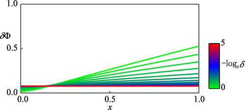
Figures 1 through 3 plot the computed normalized value function $\delta \mathrm{\Phi }=\delta \mathrm{\Phi }\left(x\right)$, the optimal control $q^{\ast }=q^{\ast }\left(x\right)$ that is the minimizer, and the optimal control ${\phi }^{\ast }={\phi }^{\ast }\left(x\right)$ that is the maximizer, against different values of the ambiguity-aversion parameter $\psi$. The computational results in these figures demonstrate that the present finite difference scheme generates numerical solutions without spurious oscillations for both large and small $\psi$, implying its satisfactory ability. Indeed, the computed value function $\mathrm{\Phi }\left(x\right)$ is non-negative and further complies with the upper- and lower-bounds (13), which are now expressed as $0\le \delta \mathrm{\Phi }\le 1$.

The computational results in Figures 1 and 2 show that both the value function $\mathrm{\Phi }$ and the optimal control $q^{\ast }$ are increasing with respect to the ambiguity-aversion parameter $\psi$. The result in Figure 2 suggests that a larger amount of the intervention with a larger deviation from the target value should be carried out when the decision-maker assumes a potentially larger ambiguity. Under the present computational condition, this dependence of $q^{\ast }$ on $\psi$ is significant only for relatively small $x$ where the growth rate of the algae population is positive. Figure 3 on the optimal control ${\phi }^{\ast }$ shows its critical dependence on the ambiguity-aversion parameter $\psi$. The computed ${\phi }^{\ast }\left(x\right)$ is decreasing with respect to both $x$ and $-\psi$, implying that the ambiguity should be assumed to be larger when the population is larger and/or the decision-maker is more ambiguity-averse. The decision-maker should not expect frequent jump disturbances for relatively large values of $\psi$. 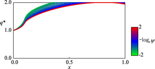The impacts of the ambiguity-aversion parameter $\psi$ on the other optimal control $q^{\ast }$ becomes more significant for larger jump intensity $\lambda \left(=0.4\right)$ as demonstrated in Figure 4. In practice, a smaller value of the ambiguity-aversion is preferred since it potentially decreases the value function, which is here considered as the optimized total cost, and also potentially decreases the deviation of the optimal control $q^{\ast }$ from the target value $q_{\text{target}}$. However, such an effort to decrease the potential ambiguity may be costly itself as well.

Figure 1. The computed normalized value function $\delta \mathrm{\Phi }$ against different values of the ambiguity-aversion parameter $\psi$. The values of $\psi$ are $\psi ={10}^{2-i/25}$ ($i=0,4,8,\dots ,100$) in the figure.

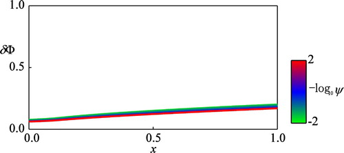
Figure 2. The computed optimal control $q^{\ast }$ against different values of the ambiguity-aversion parameter $\psi$. The values of $\psi$ are $\psi ={10}^{2-i/25}$ ($i=0,4,8,\dots ,100$) in the figure.

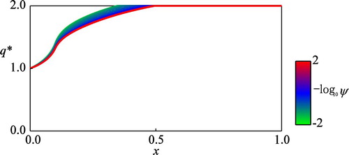
Figure 3. The computed optimal control ${\phi }^{\ast }$ against different values of the ambiguity-aversion parameter $\psi$. The values of $\psi$ are $\psi ={10}^{2-i/25}$ ($i=0,4,8,\dots ,100$) in the figure.

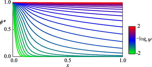
Figure 4. The computed optimal control $q^{\ast }$ against different values of the ambiguity-aversion parameter $\psi$. The same computational conditions with those in Figure 2, except for that $\lambda =0.4$ in this figure.

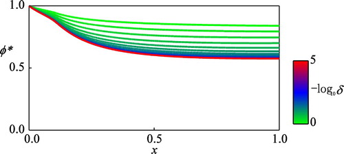
4.3.2. Dependence of the optimal controls on the discount rate

Figures 5 through 7 plot the computed normalized value function $\delta \mathrm{\Phi }=\delta \mathrm{\Phi }\left(x\right)$, the optimal control $q^{\ast }=q^{\ast }\left(x\right)$, and the optimal control ${\phi }^{\ast }={\phi }^{\ast }\left(x\right)$ against different values of the discount rate $\delta$. The computational results again imply satisfactory ability of the present scheme for handling the problems against both large and small $\delta$. In addition, the numerical solutions comply with the upper-bound (13) against all the examined values of $\delta$.

Figure 5 shows that the computed normalized value function $\delta \mathrm{\Phi }\left(x\right)$ is increasing with respect to $x$ for relatively large $\delta$, and it approaches toward a constant ($\delta \mathrm{\Phi }\approx 0.779$) as $\delta$ decreases (See, the red curve in the figure). This numerical evidence is consistent with the theory of ergodic control that the quantity $\delta \mathrm{\Phi }\left(x\right)$ approaches toward a constant called effective Hamiltonian under the vanishing-discount limit $\delta \to +0$ (Chapter 2.7 of Arapostathis et al. [5], Menaldi and Robin [52]). The effective Hamiltonian, if it exists, can be considered as the optimized following time-averaged counterpart of (10) with respect to $q$ and $\phi$: (54) $P\left(x;q,\phi \right)=\underset{T\to +\mathrm{\infty }}{lim}\frac{1}{T}\text{E}\left[{\int }_0^T\left(\text{β}\left(X_s\right)+\gamma \left(q{}_s\right)-\frac{\lambda }{\psi }\left({\phi }_s\ln {\phi }_s+1-{\phi }_s\right)\right)\text{d}s\right].$(54) Rigorous mathematical analysis of the problem under the ergodic limit is beyond the scope of this paper, in which the main difficulties are the jump-diffusion differential game structure of the problem and degeneration and nonlinearity of the coefficients. However, the computational results support the conjecture that the ergodic limit exists. Notice that this point was not addressed in the previous research [71, 72].

Figure 5. The computed normalized value function $\delta \mathrm{\Phi }$ against different values of the discount rate $\delta$. The values of $\delta$ are $\delta ={10}^{-i/20}$ ($i=0,4,8,\dots ,100$) in the figure.

Figures 6 and 7 reveal behaviour of the optimal controls under the ergodic limit numerically (See, the red curves in the figures). These figures suggest that $q^{\ast }$ and ${\phi }^{\ast }$ approach toward non-trivial limits under the ergodic limit. Firstly, on the optimal control $q^{\ast }$, Figure 6 shows that $q^{\ast }$ is decreasing with respect to $\delta$ and satisfies the condition $q^{\ast }\ge 0$, indicating that the more myopic decision-maker chooses a smaller deviation from the target value $q_{\text{target}}=1$, and vice versa. This result means that long-term management of the harmful algae population requires a larger deviation of the control variable $q$ from the target value $q_{\text{target}}$. Secondly, on the optimal control ${\phi }^{\ast }$, Figure 7 shows that ${\phi }^{\ast }$ is decreasing with respect to $\delta$ as well, indicating that longer-term management of the harmful algae population should be associated with the assumption that the jump intensity is smaller than that estimated, and vice versa. The computational results of Figures 6 and 7 are consistent with each other and practically suggest that effective suppression of the algae bloom requires larger perturbations or interventions, which should be by the jump disturbances for short-term management, while by human interventions for long-term management.

Figure 6. The computed optimal control $q^{\ast }$ against different values of the discount rate $\delta$. The values of $\delta$ are $\delta ={10}^{-i/20}$ ($i=0,4,8,\dots ,100$) in the figure.

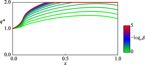
Figure 7. The computed optimal control ${\phi }^{\ast }$ against different values of the discount rate $\delta$. The values of $\delta$ are $\delta ={10}^{-i/20}$ ($i=0,4,8,\dots ,100$) in the figure.

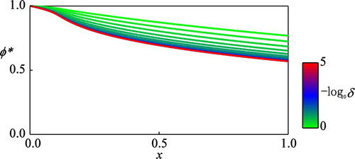
Figure 8. The computed normalized value function $\delta \mathrm{\Phi }$ against different values of the discount rate $\delta$. The same computational conditions with those in Figure 5 except for that $m=0.5$ in this figure.

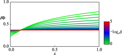
Figure 9. The computed optimal control $q^{\ast }$ against different values of the discount rate $\delta$. The same computational conditions with those in Figure 6 except for that $m=0.5$ in this figure.

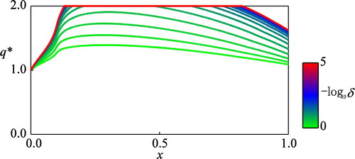
Figure 10. The computed optimal control ${\phi }^{\ast }$ against different values of the discount rate $\delta$. The same computational conditions with those in Figure 7 except for that $m=0.5$ in this figure.

It is noted that qualitatively similar conclusions are obtained for the concave $\text{β}\left(x\right)=x^m$ ($m=0.5$) as well, as demonstrated in Figures 8 through 10. In this case, the computed $\delta \mathrm{\Phi }\left(x\right)$ approaches toward a constant 0.370 as $\delta$ decreases. The decreasing property of the computed $q^{\ast }\left(x\right)$ for relatively large $x$ is considered to be due to that the increasing rate of the disutility $\text{β}\left(x\right)=x^m$ is larger in the convex case ($m=1.5$) than that in the concave case ($m=0.5$).

5. Conclusions

A stochastic control model for biological population management subject to a jump ambiguity was formulated based on the concept of multiplier-robust control, and the HJBI equation to be solved for finding the optimal management policy was derived. The HJBI equation turned out to be uniquely-solvable in a viscosity sense despite it possesses a term that is non-linear and non-local. A finite difference scheme for discretization of the equation was presented as well, which is equipped with several key properties to see convergence of numerical solutions toward the unique viscosity solution. Numerical computation of the HJBI equation focusing on an algae bloom management problem demonstrated non-trivial, state-dependent optimal population controls from both short-term and long-term viewpoint. To the authors’ knowledge, this paper is the first work that applies the multiplier-robust control approach to biological system dynamics subject to an ambiguous jump intensity. We focused on algae bloom in river environment, but the presented modelling framework can be applied to other species like biofilms on riverbed [27] and even to environmental problems where extreme jump disturbances play a central role [33] with slight modifications.

The present paper would serve as a part of a foundation for biological population management subject to model ambiguity. A limitation of this paper is that it does not consider ambiguity in the jump magnitude $g$, which is a practical issue as well. Theoretically, incorporating this ambiguity into the present model is straightforward following the existing tactic [2, 46]. However, the resulting HJBI equation may have stronger nonlinearity, which would be more difficult to be handled from both mathematical and numerical viewpoints. Extension of the present mathematical framework to spatially-distributed models would also be an important research topic when considering population migration dynamics across landscapes. Efficient description of the dynamics with a homogenization method can be helpful for this purpose [82]. Problems with multiple, interacting species can be handled within the present mathematical framework with appropriate extensions. Analyzing advanced problems, like impulse and singular controls, is also interesting. Based on related mathematical frameworks of stochastic control under ambiguity, the authors have considered impulsive observation/control of stochastic population dynamics (e.g. the stochastic control models under partial observations [73, 74]). They can be effectively combined with the presented model to formulate a more realistic model concurrently considering impulsive and continuous-time control variables under ambiguity.

Acknowledgement

The authors thank the two reviewers for their critical comments and helpful suggestions.

Disclosure statement

No potential conflict of interest was reported by the author(s).

Additional information

Funding

JSPS [Japan Society for the Promotion of Science] Research Grant 17K15345 and 18K01714 support this research.

Appendix A

Proofs of the lemmas and propositions in the main text are described in this appendix.

Proof of Lemma 2.1

The proof here is based on the proof of Theorem 2.2 of Lungu and Øksendal [49], but several changes are made to handle the controlled jump-diffusion process.

Fix admissible $q\in \mathcal{Q}$ and $\phi \in \mathcal{A}$. Consider the auxiliary SDE (55) $\text{d}{X}_t=A_1\left(X_t\right)\text{d}t+A_2\left(X_t\right)\text{d}{B}_t-X_{t-}\text{d}{\tilde{P}}_t,t>0$(55) with (56) $A_1\left(X_t\right)=-\alpha \left(q_t\right)X_t+r\left({\tilde{X}}_t\right){\tilde{X}}_t\left(1-\frac{{\tilde{X}}_t}{K\left(q_t\right)}\right)$(56) and (57) $A_2\left(X_t\right)=\sigma max\left(X_t\left(1-\frac{X_t}{K\left(q_t\right)}\right),0\right),$(57) where ${\tilde{X}}_t=max\left\{0,min\left\{X_t,K_{max}\right\}\right\}$. By Theorem 4.58 of Capasso and Bakstein [18], the SDE (55) admits a unique strong solution.

Now, we show that this solution is valued in $\mathrm{\Omega }$. Assume $0<x<K_{max}$. Set the stopping time $\tau =inf\left\{t|t>0,X_t=0\text{ or }{K}_{max}\right\}$. Assume $X_{\tau }=0$. For $0<t<\tau$, $0<X_t={\tilde{X}}_t<K_{max}$ and we can define $Y_t=\ln X_t$ in this interval. Applying the Itô’s lemma to $Y_t$ ($0<t<\tau$) yields (58) $\begin{array}{rl}\text{d}{Y}_t& =\frac{\text{d}{X}_t}{X_t}-\frac{{\left(\text{d}{X}_t\right)}^2}{2{\left(X_t\right)}^2}+\left(\ln X_t-\ln X_{t-}\right)\text{d}{\tilde{N}}_t\\ & =A_3\left(X_t\right)\text{d}t+A_4\left(X_t\right)\text{d}{B}_t+\text{d}{I}_t\end{array}$(58) with (59) $\begin{array}{rl}{A}_3\left(X_t\right)& =r\left(X_t\right)\left(1-\frac{X_t}{K\left(q_t\right)}\right)-\alpha \left(q_t\right)-\frac{{\sigma }^2}{2}{\left(max\left\{1-\frac{X_t}{K\left(q_t\right)},0\right\}\right)}^2,\end{array}$(59) (60) $\begin{array}{rl}{A}_4\left(X_t\right)& =\sigma max\left\{1-\frac{X_t}{K\left(q_t\right)},0\right\},\end{array}$(60) and (61) $I_t={\int }_0^t\left(\ln X_s-\ln X_{s-}\right)\text{d}{\tilde{N}}_s=\sum _{k=1}^{{\tilde{N}}_t}\ln \left(1-z_k\right).$(61) Then, we have (62) $\ln X_t=\ln x+{\int }_0^t\left(A_3\left(X_s\right)\text{d}s+A_4\left(X_s\right)\text{d}{B}_s\right)+I_t,0<t<\tau .$(62) The left-hand side of (62) diverges toward $-\mathrm{\infty }$ as $t\uparrow \tau$. On the other hand, the last term in the right-hand side is bounded or diverges to $+\mathrm{\infty }$ as $t\uparrow \tau$. The same is true for the second term. In any case, the limits of the left- and right-hand sides do not coincide, which is a contradiction. Therefore, we must have $\tau =+\mathrm{\infty }$, showing that $X_t>0$.

In an essentially similar manner, by considering the process $Z_t=\ln \left(K_{max}-X_t\right)$, we can show $X_t<K_{max}$. Assume $X_{\tau }=K_{max}$. Applying the Itô’s lemma to $Y_t$ ($0<t<\tau$) yields (63) $\begin{array}{rl}\text{d}{Z}_t& =-\frac{\text{d}{X}_t}{K_{max}-X_t}-\frac{{\left(\text{d}{X}_t\right)}^2}{2{\left(K_{max}-X_t\right)}^2}\text{ + d}{J}_t\\ & =A_5\left(X_t\right)\text{d}t+A_6\left(X_t\right)\text{d}{B}_t+\text{d}{J}_t\end{array}$(63) with (64) $\begin{array}{rl}{A}_5\left(X_t\right)& =-\frac{r\left(X_t\right)X_t}{K\left(q_t\right)}\frac{K\left(q_t\right)-X_t}{K_{max}-X_t}+\alpha \left(q_t\right)\frac{X_t}{K_{max}-X_t}-\frac{{\sigma }^2{X}_t^2}{2K{\left(q_t\right)}^2}\frac{max{\left\{K\left(q_t\right)-X_t,0\right\}}^2}{{\left(K_{max}-X_t\right)}^2},\end{array}$(64) (65) $\begin{array}{rl}{A}_6\left(X_t\right)& =-\sigma \frac{X_t}{K\left(q_t\right)}\frac{max\left\{K\left(q_t\right)-X_t,0\right\}}{K_{max}-X_t},\end{array}$(65) and (66) $\begin{array}{rl}{J}_t& ={\int }_0^t\left(\ln \left(K_{max}-X_s\right)-\ln \left(K_{max}-X_{s-}\right)\right)\text{d}{\tilde{N}}_s\\ & =\sum _{k=1}^{{\tilde{N}}_t}\ln \frac{K_{max}-X_{{\tau }_k}}{K_{max}-X_{{\tau }_k-0}}\\ & =\sum _{k=1}^{{\tilde{N}}_t}\ln \left(1+\frac{z_k{X}_{{\tau }_k-0}}{K_{max}-X_{{\tau }_k-0}}\right)\\ & \ge 0.\end{array}$(66) Notice that (67) $A_5\left(X_t\right)\ge -\frac{r\left(X_t\right)K_{max}}{K\left(q_t\right)}+\alpha \left(q_t\right)\frac{X_t}{K_{max}-X_t}-\frac{{\sigma }^2{K}_{max}^2}{2K{\left(q_t\right)}^2}$(67) and (68) $\begin{array}{rl}|A_6\left(X_t\right)|& =\sigma \frac{X_t}{K\left(q_t\right)}\frac{max\left\{K\left(q_t\right)-X_t,0\right\}}{K_{max}-X_t}\\ & \le \sigma \frac{K_{max}}{K\left(q_t\right)}\\ & <+\mathrm{\infty }.\end{array}$(68) We then obtain (69) $\ln \left(K_{max}-X_t\right)=\ln x+{\int }_0^t\left(A_5\left(X_s\right)\text{d}s+A_6\left(X_s\right)\text{d}{B}_s\right)+J_t,0<t<\tau .$(69) The left-hand side of (69) diverges toward $-\mathrm{\infty }$ as $t\uparrow \tau$. On the other hand, the right-hand side is bounded or diverges to $+\mathrm{\infty }$ as $t\uparrow \tau$. Then, the limits of the left and right-hand sides do not coincide, which is a contradiction. Therefore, we must have $\tau =+\mathrm{\infty }$, showing that $X_t<K_{max}$.

Consequently, we have $0<X_t<K_{max}$ if $0<x<K_{max}$. The cases $x=0,K_{max}$ are trivial. Then, it follows that the solution to the SDE (55) is valued in $\mathrm{\Omega }$. Under this condition, the SDE (55) is identical to (6). The proof is thus completed.

Proof of Lemma 3.1

We use a similar methodology with Yoshioka and Tsujimura [73]. The solution to the SDE (6) with the initial condition $x_i$ is denoted as $X_t^{\left(i\right)}$ ($i=1,2$). Based on the argument in the proof of Lemma 3.1 of Bayraktar et al. [10], combined with Lemma 2.1, we obtain the estimate (70) $\text{E}\left[|X_t^{\left(1\right)}-X_t^{\left(2\right)}|\right]\le exp\left(C_{1}t\right)|x_1-x_2|,t\ge 0$(70) with a constant $C_1>0$. Choose an admissible pair $\left(q,\phi \right)$. Then, by (10) and the Hölder continuity of $\text{β}$, we obtain (71) $\begin{array}{rl}|P\left(x_1;q,\phi \right)-P\left(x_2;q,\phi \right)|& =\text{E}\left[{\int }_0^{\mathrm{\infty }}{e}^{-\delta s}|\text{β}\left(X_s^{\left(1\right)}\right)-\text{β}\left(X_s^{\left(2\right)}\right)|\text{d}s\right]\\ & \le C_2\text{E}\left[{\int }_0^{\mathrm{\infty }}{e}^{-\delta s}{|X_s^{\left(1\right)}-X_s^{\left(2\right)}|}^m\text{d}s\right]\\ & =C_2{\int }_0^{\mathrm{\infty }}{e}^{-\delta s}\text{E}\left[{|X_s^{\left(1\right)}-X_s^{\left(2\right)}|}^m\right]\text{d}s\end{array}$(71) with a constant $C_2>0$. We have (72) $\begin{array}{rl}|X_s^{\left(1\right)}-X_s^{\left(2\right)}{|}^m& \le |X_s^{\left(1\right)}-X_s^{\left(2\right)}{|}^{m-1}|X_s^{\left(1\right)}-X_s^{\left(2\right)}|\\ & \le K_{max}^{m-1}|X_s^{\left(1\right)}-X_s^{\left(2\right)}|\end{array}$(72) if $m\ge 1$ by Lemma 2.1 and (73) $\text{E}\left[{|X_s^{\left(1\right)}-X_s^{\left(2\right)}|}^m\right]\le (\text{E}\left[|X_s^{\left(1\right)}-X_s^{\left(2\right)}|\right]{)}^m$(73) if $0<m<1$ by the classical Jensen’s inequality. Now, we consider the three cases (a) through (c): (a) $\delta >C_1$, (b) $\delta <C_1$, and (c) $\delta =C_1$.

• (a) $\delta >C_1$

In this case, we arrive at (74) $\begin{array}{rl}|P\left(x_1;q,\phi \right)-P\left(x_2;q,\phi \right)|& \le C_2{K}_{max}^{m-1}{\int }_0^{\mathrm{\infty }}{e}^{-\delta s}{e}^{C_{1}s}|x_1-x_2|\text{d}s\\ & =\frac{C_2{K}_{max}^{m-1}}{\delta -C_1}|x_1-x_2|\end{array}$(74) if $m\ge 1$ and (75) $\begin{array}{rl}|P\left(x_1;q,\phi \right)-P\left(x_2;q,\phi \right)|& \le C_2{\int }_0^{\mathrm{\infty }}{e}^{-\delta s}{\left(\text{E}\left[|X_s^{\left(1\right)}-X_s^{\left(2\right)}|\right]\right)}^m\text{d}s\\ & \le C_2{\int }_0^{\mathrm{\infty }}{e}^{-\delta s}{e}^{m{C}_{1}s}{|x_1-x_2|}^m\text{d}s\\ & =\frac{C_2}{\delta -m{C}_1}|x_1-x_2{|}^m\end{array}$(75) if $0<m<1$. Consequently, we obtain (76) $|P\left(x_1;q,\phi \right)-P\left(x_2;q,\phi \right)|\le C|x_1-x_2{|}^{min\left\{1,m\right\}}$(76) with a constant $C>0$ and thus (77) $P\left(x_1;q,\phi \right)\le C|x_1-x_2{|}^{min\left\{1,m\right\}}+P\left(x_2;q,\phi \right).$(77) This inequality leads to (78) $\begin{array}{rl}P\left(x_1;q,\phi \right)& \le C|x_1-x_2{|}^{min\left\{1,m\right\}}+\underset{\phi \in \mathcal{A}}{sup}P\left(x_2;q,\phi \right),\end{array}$(78) (79) $\begin{array}{rl}\underset{\phi \in \mathcal{A}}{sup}P\left(x_1;q,\phi \right)& \le C|x_1-x_2{|}^{min\left\{1,m\right\}}+\underset{\phi \in \mathcal{A}}{sup}P\left(x_2;q,\phi \right),\end{array}$(79) (80) $\begin{array}{rl}\underset{q\in \mathcal{Q}}{inf}\underset{\phi \in \mathcal{A}}{sup}P\left(x_1;q,\phi \right)& \le C|x_1-x_2{|}^{min\left\{1,m\right\}}+\underset{\phi \in \mathcal{A}}{sup}P\left(x_2;q,\phi \right),\end{array}$(80) (81) $\begin{array}{rl}\underset{q\in \mathcal{Q}}{inf}\underset{\phi \in \mathcal{A}}{sup}P\left(x_1;q,\phi \right)& \le C|x_1-x_2{|}^{min\left\{1,m\right\}}+\underset{q\in \mathcal{Q}}{inf}\underset{\phi \in \mathcal{A}}{sup}P\left(x_2;q,\phi \right),\end{array}$(81) and thus (82) $\mathrm{\Phi }\left(x_1\right)\le C|x_1-x_2{|}^{min\left\{1,m\right\}}+\mathrm{\Phi }\left(x_2\right).$(82) In a symmetrical way, we obtain (83) $\mathrm{\Phi }\left(x_2\right)\le C|x_1-x_2{|}^{min\left\{1,m\right\}}+\mathrm{\Phi }\left(x_1\right).$(83)

Combining (82) and (83) completes the proof for the case (a).

• (b) $\delta <C_1$

Firstly, assume $m\ge 1$. By Lemma 2.1, combining (70) through (72) leads to the inequality (84) $\begin{array}{rl}|P\left(x_1;q,\phi \right)-P\left(x_2;q,\phi \right)|& \le C_2{\int }_0^{\mathrm{\infty }}{e}^{-\delta s}\text{E}\left[{|X_s^{\left(1\right)}-X_s^{\left(2\right)}|}^m\right]\text{d}s\\ & \le C_2{K}_{max}^{m-1}{\int }_0^{\mathrm{\infty }}{e}^{-\delta s}\text{E}\left[|X_s^{\left(1\right)}-X_s^{\left(2\right)}|\right]\text{d}s\\ & \le C_2{K}_{max}^{m-1}{\int }_0^{\mathrm{\infty }}{e}^{-\delta s}\text{min}\left\{\text{E}\left[|X_s^{\left(1\right)}-X_s^{\left(2\right)}|\right],K_{max}\right\}\text{d}s\\ & \le C_2{K}_{max}^{m-1}{\int }_0^{\mathrm{\infty }}{e}^{-\delta s}min\left\{e^{C_{1}s}|x_1-x_2|,K_{max}\right\}\text{d}s\\ & =C_2{K}_{max}^m{\int }_0^{\mathrm{\infty }}{e}^{-\delta s}min\left\{e^{C_{1}s}\omega ,1\right\}\text{d}s\end{array}$(84) with $\omega =\frac{|x_1-x_2|}{K_{max}}$ since $\text{E}\left[|X_s^{\left(1\right)}-X_s^{\left(2\right)}|\right]\le K_{max}$. If $0<m<1$, then in a similar manner, we have (85) $\begin{array}{rl}|P\left(x_1;q,\phi \right)-P\left(x_2;q,\phi \right)|& \le C_2{\int }_0^{\mathrm{\infty }}{e}^{-\delta s}\text{E}\left[{|X_s^{\left(1\right)}-X_s^{\left(2\right)}|}^m\right]\text{d}s\\ & \le C_2{\int }_0^{\mathrm{\infty }}{e}^{-\delta s}{\left(\text{E}\left[|X_s^{\left(1\right)}-X_s^{\left(2\right)}|\right]\right)}^m\text{d}s\\ & \le C_2{\int }_0^{\mathrm{\infty }}{e}^{-\delta s}\text{min}\left\{{\left(\text{E}\left[|X_s^{\left(1\right)}-X_s^{\left(2\right)}|\right]\right)}^m,K_{max}^m\right\}\text{d}s\\ & \le C_2{\int }_0^{\mathrm{\infty }}{e}^{-\delta s}min\left\{e^{m{C}_{1}s}{|x_1-x_2|}^m,K_{max}^m\right\}\text{d}s\\ & =K_{max}^m{\int }_0^{\mathrm{\infty }}{e}^{-\delta s}min\left\{e^{m{C}_{1}s}{\omega }^m,1\right\}\text{d}s.\end{array}$(85) We can assume $|x_1-x_2|>0$, otherwise the statement of the proposition is trivial. Set (86) $s_0=\frac{1}{\delta }\ln \frac{1}{\omega }.$(86) The integral in the last term of (84) is calculated as (87) $\begin{array}{rl}{\int }_0^{\mathrm{\infty }}{e}^{-\delta s}min\left\{e^{C_{1}s}\omega ,1\right\}\text{d}s& ={\int }_0^{s_0}{e}^{-\delta s}{e}^{C_{1}s}\omega \text{d}s+{\int }_{s_0}^{\mathrm{\infty }}{e}^{-\delta s}\text{d}s\\ & =\frac{\omega }{C_1-\delta }\left(e^{\left(C_1-\delta \right)s_0}-1\right)+\frac{1}{\delta }{e}^{-\delta s_0}.\end{array}$(87) Substituting (86) into (87) yields (88) ${\int }_0^{\mathrm{\infty }}{e}^{-\delta s}min\left\{e^{C_{1}s}\omega ,1\right\}\text{d}s=-\frac{\omega }{C_1-\delta }+\frac{C_1}{\delta \left(C_1-\delta \right)}{\omega }^{\frac{C_1}{\delta }}.$(88) Similarly, the integral in the last term of (85) is calculated as (89) ${\int }_0^{\mathrm{\infty }}{e}^{-\delta s}min\left\{e^{m{C}_{1}s}{\omega }^m,1\right\}\text{d}s=-\frac{{\omega }^m}{m{C}_1-\delta }+\frac{C_1}{\delta \left(m{C}_1-\delta \right)}{\omega }^{\frac{2m{C}_1}{\delta }}.$(89) The right-hand sides of (88) and (89) are continuous with respect to $\omega$ and thus to $|x_1-x_2|$, and vanish when $|x_1-x_2|=0$. Therefore, for both $m\ge 1$ and $0<m<1$, we obtain (90) $|P\left(x_1;q,\phi \right)-P\left(x_2;q,\phi \right)|\le c\left(|x_1-x_2|\right).$(90)

Application of the discussion in case (a) to (90) completes the proof for the case (b).

• (c) $\delta =C_1$

A straightforward calculation same with that in case (b) leads to the estimate (91) $|P\left(x_1;q,\phi \right)-P\left(x_2;q,\phi \right)|\le C_3\frac{{\omega }^{min\left\{1,m\right\}}}{\delta }\left(1+min\left\{1,m\right\}\ln \frac{1}{\omega }\right)$(91) with a constant $C_3>0$. Application of the discussion in case (a) to (90) completes the proof for the case (c).

Proof of Proposition 3.1

The proof is based on Theorem 9.8 of Øksendal and Sulem [58] with the help of the monotonicity (25).

Firstly, we show that the value function is a viscosity super-solution. Set a test function $\varphi$ for viscosity super-solutions ($\varphi -\mathrm{\Phi }$ is globally maximized at $x$, $\varphi \left(x\right)=\mathrm{\Phi }\left(x\right)$, $\varphi \le \mathrm{\Phi }$ on $\mathrm{\Omega }$). By the dynamic programming principle, for any stopping time $\tau >0$ adapted to the filtration $\mathcal{F}$, we have (92) $\mathrm{\Phi }\left(x\right)=\underset{q\in \mathcal{Q}}{inf}\underset{\phi \in \mathcal{A}}{sup}\text{E}\left[{\int }_0^{\hat{\tau }}{e}^{-\delta s}\left(\text{β}\left(X_s\right)+\gamma \left(q_s\right)-\frac{\lambda }{\psi }\left({\phi }_s\ln {\phi }_s+1-{\phi }_s\right)\right)\text{d}s+e^{-\delta \hat{\tau }}\mathrm{\Phi }\left(X_{\hat{\tau }}\right)\right]$(92) with $\hat{\tau }=min\left(\tau ,\rho \right)$ and a constant $\rho >0$. Fix one admissible $\epsilon$-optimal control $q^{\left(\epsilon \right)}$ ($\epsilon >0$) such that (93) $\mathrm{\Phi }\left(x\right)\ge \underset{\phi \in \mathcal{A}}{sup}\text{E}\left[{\int }_0^{\hat{\tau }}{e}^{-\delta s}\left(\text{β}\left(X_s\right)+\gamma \left(q_s^{\left(\epsilon \right)}\right)-\frac{\lambda }{\psi }\left({\phi }_s\ln {\phi }_s+1-{\phi }_s\right)\right)\text{d}s+e^{-\delta \hat{\tau }}\mathrm{\Phi }\left(X_{\hat{\tau }}\right)\right]-\rho \epsilon .$(93) By Definition 3.1(b), since $\mathrm{\Phi }\ge \varphi$ in $\mathrm{\Omega }$, we obtain the inequality (94) $\begin{array}{rl}\mathrm{\Phi }\left(x\right)\ge & \underset{\phi \in \mathcal{A}}{sup}\text{E}\left[{\int }_0^{\hat{\tau }}{e}^{-\delta s}\left(\text{β}\left(X_s\right)+\gamma \left(q_s^{\left(\epsilon \right)}\right)-\frac{\lambda }{\psi }\left({\phi }_s\ln {\phi }_s+1-{\phi }_s\right)\right)\text{d}s+e^{-\delta \hat{\tau }}\varphi \left(X_{\hat{\tau }}\right)\right]-\rho \epsilon \\ \ge & \varphi \left(x\right)+\underset{\phi \in \mathcal{A}}{sup}\text{E}\left[{\int }_0^{\hat{\tau }}{e}^{-\delta s}\left(-L_{q_s^{\left(\epsilon \right)}}\varphi \left(X_s\right)-I_{{\phi }_s}\varphi +\text{β}\left(X_s\right)+\gamma \left(q_s^{\left(\epsilon \right)}\right)\right)\text{d}s\right]-\rho \epsilon \end{array}$(94) by an application of the classical Dynkin’s formula to $e^{-\delta s}\varphi \left(X_s\right)$. Then, since $\mathrm{\Phi }\left(x\right)=\varphi \left(x\right)$, (94) leads to (95) $-\underset{\phi \in \mathcal{A}}{sup}\text{E}\left[{\int }_0^{\hat{\tau }}{e}^{-\delta s}\left(-L_{q_s^{\left(\epsilon \right)}}\varphi \left(X_s\right)-I_{{\phi }_s}\varphi +\text{β}\left(X_s\right)+\gamma \left(q_s^{\left(\epsilon \right)}\right)\right)\text{d}s\right]\ge -\rho \epsilon .$(95) Divided by $\text{E}\left[\hat{\tau }\right]$ and taking the limit $\rho \to +0$ in (95) gives (96) $L_{q_0^{\left(\epsilon \right)}}\varphi \left(x\right)-\text{β}\left(x\right)-\gamma \left(q_0^{\left(\epsilon \right)}\right)+\underset{\phi >0}{inf}{I}_{\phi }\varphi \ge -\rho \epsilon .$(96) Since $\epsilon$ is arbitrary, we have (97) $L_{q_0^{\left(0\right)}}\varphi \left(x\right)-\gamma \left(q_0^{\left(0\right)}\right)+\underset{\phi >0}{inf}{I}_{\phi }\varphi -\text{β}\left(x\right)\ge 0.$(97) and thus (98) $\begin{array}{rl}\underset{q\in Q}{sup}\left\{L_q\varphi \left(x\right)-\gamma \left(q\right)-\text{β}\left(x\right)\right\}+\underset{\phi >0}{inf}{I}_{\phi }\varphi & =\delta \varphi \left(x\right)+H\left(x,\frac{\text{d}\varphi }{\text{d}x}\left(x\right),\frac{{\text{d}}^2\varphi }{\text{d}{x}^2}\left(x\right)\right)+\frac{\lambda }{\psi }\left(1-e^{-\psi \mathrm{\Delta }\varphi \left(x\right)}\right).\\ & =\delta \varphi \left(x\right)+H\left(x,\frac{\text{d}\varphi }{\text{d}x}\left(x\right),\frac{{\text{d}}^2\varphi }{\text{d}{x}^2}\left(x\right)\right)+\frac{\lambda }{\psi }\left(1-e^{-\psi \mathrm{\Delta }\varphi \left(x\right)}\right)\\ & \ge 0\end{array}$(98) Application of Proposition 3 of Azimzadeh et al. [6] with the help of the monotonicity (25) to (98) yields the desired inequality. (99) $\delta \mathrm{\Phi }\left(x\right)+H\left(x,\frac{\text{d}\varphi }{\text{d}x}\left(x\right),\frac{{\text{d}}^2\varphi }{\text{d}{x}^2}\left(x\right)\right)+\frac{\lambda }{\psi }\left(1-e^{-\psi \mathrm{\Delta }\mathrm{\Phi }\left(x\right)}\right)\ge 0.$(99) Secondly, we show that the value function is a viscosity sub-solution. Set a test function $\varphi$ for viscosity sub-solutions ($\varphi -\mathrm{\Phi }$ is globally minimized at $x$, $\varphi \left(x\right)=\mathrm{\Phi }\left(x\right)$, $\varphi \ge \mathrm{\Phi }$ on $\mathrm{\Omega }$). For any admissible $q$, we have (100) $\begin{array}{rl}\mathrm{\Phi }\left(x\right)& \le \underset{\phi \in \mathcal{A}}{sup}\text{E}\left[{\int }_0^{\hat{\tau }}{e}^{-\delta s}\left(\text{β}\left(X_s\right)+\gamma \left(q_s\right)-\frac{\lambda }{\psi }\left({\phi }_s\ln {\phi }_s+1-{\phi }_s\right)\right)\text{d}s+e^{-\delta \hat{\tau }}\mathrm{\Phi }\left(X_{\hat{\tau }}\right)\right]\\ & \le \underset{\phi \in \mathcal{A}}{sup}\text{E}\left[{\int }_0^{\hat{\tau }}{e}^{-\delta s}\left(\text{β}\left(X_s\right)+\gamma \left(q_s\right)-\frac{\lambda }{\psi }\left({\phi }_s\ln {\phi }_s+1-{\phi }_s\right)\right)\text{d}s+e^{-\delta \hat{\tau }}\varphi \left(X_{\hat{\tau }}\right)\right]\\ & =\varphi \left(x\right)+\underset{\phi \in \mathcal{A}}{sup}\text{E}\left[{\int }_0^{\hat{\tau }}{e}^{-\delta s}\left(-L_{q_s}\varphi \left(X_s\right)-I_{{\phi }_s}\varphi +\text{β}\left(X_s\right)+\gamma \left(q_s\right)\right)\text{d}s\right].\end{array}$(100) again by the Dynkin’s formula and Definition 3.1(a). Then, as in the proof for viscosity super-solutions, we have (101) $L_q\varphi \left(x\right)-\text{β}\left(x\right)-\gamma \left(q\right)+\underset{\phi >0}{inf}{I}_{\phi }\varphi \le 0.$(101) Since $q$ is arbitrary, we have (102) $\delta \varphi \left(x\right)+H\left(x,\frac{\text{d}\varphi }{\text{d}x}\left(x\right),\frac{{\text{d}}^2\varphi }{\text{d}{x}^2}\left(x\right)\right)+\frac{\lambda }{\psi }\left(1-e^{-\psi \mathrm{\Delta }\varphi \left(x\right)}\right)\le 0.$(102) Finally, application of Proposition 3 of Azimzadeh et al. [6] with the help of the monotonicity (25) to (102) yields the desired inequality. (103) $\delta \mathrm{\Phi }\left(x\right)+H\left(x,\frac{\text{d}\varphi }{\text{d}x}\left(x\right),\frac{{\text{d}}^2\varphi }{\text{d}{x}^2}\left(x\right)\right)+\frac{\lambda }{\psi }\left(1-e^{-\psi \mathrm{\Delta }\mathrm{\Phi }\left(x\right)}\right)\le 0.$(103) Combining (99) and (103) completes the proof.

Proof of Proposition 3.2

As in the standard argument for comparison theorems [24], it is sufficient to show that for any couple of a viscosity sub-solution $\underset{\_}{\mathrm{\Phi }}$ and a viscosity super-solution $\overline{\mathrm{\Phi }}$, we have $\overline{\mathrm{\Phi }}\ge \underset{\_}{\mathrm{\Phi }}$ in $\mathrm{\Omega }$. As stated in Proposition 3.1, the HJBI equation (24) is solved in $\mathrm{\Omega }$, namely both the inside and boundaries of the compact domain, without imposing any boundary conditions. In this sense, the proof is actually simpler than the standard ones.

Assume $\underset{\mathrm{\Omega }}{sup}\left\{\underset{\_}{\mathrm{\Phi }}-\overline{\mathrm{\Phi }}\right\}>0$. Set $f_{\epsilon }\left(x,y\right)=\underset{\_}{\mathrm{\Phi }}\left(x\right)-\overline{\mathrm{\Phi }}\left(y\right)-{\varphi }_{\epsilon }\left(x,y\right)$ with ${\varphi }_{\epsilon }\left(x,y\right)=\frac{1}{2\epsilon }(x-y{)}^2$ in $\mathrm{\Omega }\times \mathrm{\Omega }$. This $f_{\epsilon }$ attains a maximum at some point in $\mathrm{\Omega }\times \mathrm{\Omega }$ because it is upper semi-continuous. The maximizer of $f_{\epsilon }$ is denoted as $\left(x_{\epsilon },y_{\epsilon }\right)\in \mathrm{\Omega }\times \mathrm{\Omega }$. Then, we have (104) $f_{\epsilon }\left(x_{\epsilon },y_{\epsilon }\right)\ge f_{\epsilon }\left(x,x\right)=\underset{\_}{\mathrm{\Phi }}\left(x\right)-\overline{\mathrm{\Phi }}\left(x\right)\text{for}\text{all}x\in \mathrm{\Omega }.$(104) Following the standard argument [24], we can choose a sequence $\epsilon ={\epsilon }_k$ with $\underset{k\to +\mathrm{\infty }}{lim}{\epsilon }_k=0$ such that (105) $\underset{k\to +\mathrm{\infty }}{lim}{x}_{{\epsilon }_k}=\underset{k\to +\mathrm{\infty }}{lim}{y}_{{\epsilon }_k}=x_0$(105) and (106) $\underset{k\to +\mathrm{\infty }}{lim}\frac{1}{{\epsilon }_k}(x_{{\epsilon }_k}-y_{{\epsilon }_k}{)}^2=0$(106) with some $x_0\in \mathrm{\Omega }$ such that $\underset{\_}{\mathrm{\Phi }}\left(x_0\right)-\overline{\mathrm{\Phi }}\left(x_0\right)=\underset{\mathrm{\Omega }}{sup}\left\{\underset{\_}{\mathrm{\Phi }}-\overline{\mathrm{\Phi }}\right\}>0$. Then, we have (107) $\underset{\_}{\mathrm{\Phi }}\left(x_0\right)-\overline{\mathrm{\Phi }}\left(x_0\right)\ge \underset{\_}{\mathrm{\Phi }}\left(x\right)-\overline{\mathrm{\Phi }}\left(x\right)$(107) and thus (108) $\overline{\mathrm{\Phi }}\left(x\right)-\underset{\_}{\mathrm{\Phi }}\left(x\right)\ge \overline{\mathrm{\Phi }}\left(x_0\right)-\underset{\_}{\mathrm{\Phi }}\left(x_0\right)$(108) for all $x\in \mathrm{\Omega }$. Hereafter, we only consider such a sub-sequence. We see that $\underset{\_}{\mathrm{\Phi }}\left(x\right)-\left(\overline{\mathrm{\Phi }}\left(y_{\epsilon }\right)+{\varphi }_{\epsilon }\left(x,y_{\epsilon }\right)\right)$ is maximized at $x_{\epsilon }$ and $\overline{\mathrm{\Phi }}\left(y\right)-\left(\underset{\_}{\mathrm{\Phi }}\left(x_{\epsilon }\right)-{\varphi }_{\epsilon }\left(x_{\epsilon },y\right)\right)$ is minimized at $y_{\epsilon }$. Therefore, we can use $\underset{\_}{\mathrm{\Phi }}\left(x_{\epsilon }\right)+{\varphi }_{\epsilon }\left(x,y_{\epsilon }\right)-{\varphi }_{\epsilon }\left(x_{\epsilon },y_{\epsilon }\right)$ as a test function for the viscosity sub-solution and $\overline{\mathrm{\Phi }}\left(y_{\epsilon }\right)-{\varphi }_{\epsilon }\left(x_{\epsilon },y\right)+{\varphi }_{\epsilon }\left(x_{\epsilon },y_{\epsilon }\right)$ as a test function for the viscosity super-solution, respectively.

Set $p_{\epsilon }=\frac{x_{\epsilon }-y_{\epsilon }}{\epsilon }$. By Ishiis’ lemma (Section 3 of Crandall et al. [24]), there exist $M_1,M_2$ such that (109) $\begin{array}{rl}& -\frac{3}{\epsilon }\left(\begin{array}{cc}1& 0\\ 0& 1\end{array}\right)\le \left(\begin{array}{cc}{M}_1& 0\\ 0& -M_2\end{array}\right)\le \frac{3}{\epsilon }\left(\begin{array}{cc}1& -1\\ -1& 1\end{array}\right),\end{array}$(109) (110) $\begin{array}{rl}& \delta \underset{\_}{\mathrm{\Phi }}\left(x_{\epsilon }\right)+H\left(x_{\epsilon },p_{\epsilon },M_1\right)+\frac{\lambda }{\psi }\left(1-e^{-\psi \mathrm{\Delta }\underset{\_}{\mathrm{\Phi }}\left(x_{\epsilon }\right)}\right)\le 0,\end{array}$(110) and (111) $\delta \overline{\mathrm{\Phi }}\left(y_{\epsilon }\right)+H\left(y_{\epsilon },p_{\epsilon },M_2\right)+\frac{\lambda }{\psi }\left(1-e^{-\psi \mathrm{\Delta }\overline{\mathrm{\Phi }}\left(y_{\epsilon }\right)}\right)\ge 0.$(111) Combining (110) and (111) yields (112) $\delta \left(\underset{\_}{\mathrm{\Phi }}\left(x_{\epsilon }\right)-\overline{\mathrm{\Phi }}\left(y_{\epsilon }\right)\right)-e^{-\psi \mathrm{\Delta }\underset{\_}{\mathrm{\Phi }}\left(x_{\epsilon }\right)}+e^{-\psi \mathrm{\Delta }\overline{\mathrm{\Phi }}\left(y_{\epsilon }\right)}\le H\left(y_{\epsilon },p_{\epsilon },M_2\right)-H\left(x_{\epsilon },p_{\epsilon },M_1\right).$(112) By the structure condition ((3.21) and Section 3.3.2 of Koike [40]), which is fulfilled by the Hamiltonian $H$, a straightforward calculation shows that there exists a non-negative and continuous function $c$ in $\mathrm{\Omega }$ with $c\left(0\right)=0$ such that (113) $|H\left(y_{\epsilon },p_{\epsilon },M_2\right)-H\left(x_{\epsilon },p_{\epsilon },M_1\right)|\le c\left(\epsilon p_{\epsilon }\left(1+p_{\epsilon }\right)\right).$(113) Therefore, (112) with (113) leads to (114) $\delta \left(\underset{\_}{\mathrm{\Phi }}\left(x_{\epsilon }\right)-\overline{\mathrm{\Phi }}\left(y_{\epsilon }\right)\right)-e^{-\psi \mathrm{\Delta }\underset{\_}{\mathrm{\Phi }}\left(x_{\epsilon }\right)}+e^{-\psi \mathrm{\Delta }\overline{\mathrm{\Phi }}\left(y_{\epsilon }\right)}\le c\left(\epsilon p_{\epsilon }\left(1+p_{\epsilon }\right)\right).$(114) Letting $\epsilon \to +0$ in (110) and (111) yields $\epsilon p_{\epsilon }\left(1+p_{\epsilon }\right)\to 0$ by (106), and thus (115) $\delta \left(\underset{\_}{\mathrm{\Phi }}\left(x_0\right)-\overline{\mathrm{\Phi }}\left(x_0\right)\right)-e^{-\psi \mathrm{\Delta }\underset{\_}{\mathrm{\Phi }}\left(x_0\right)}+e^{-\psi \mathrm{\Delta }\overline{\mathrm{\Phi }}\left(x_0\right)}\le 0.$(115) The assumption $\overline{\mathrm{\Phi }}\left(x_0\right)-\underset{\_}{\mathrm{\Phi }}\left(x_0\right)<0$ gives (116) $0<e^{-\psi \mathrm{\Delta }\underset{\_}{\mathrm{\Phi }}\left(x_0\right)}-e^{-\psi \mathrm{\Delta }\overline{\mathrm{\Phi }}\left(x_0\right)}$(116) and thus (117) $-\psi \mathrm{\Delta }\overline{\mathrm{\Phi }}\left(x_0\right)<-\psi \mathrm{\Delta }\underset{\_}{\mathrm{\Phi }}\left(x_0\right),$(117) which can be rearranged as (118) $\overline{\mathrm{\Phi }}\left(x_0\right)-{\int }_0^{1}g\left(z\right)\overline{\mathrm{\Phi }}\left(\left(1-z\right)x_0\right)\text{d}z>\underset{\_}{\mathrm{\Phi }}\left(x_0\right)-{\int }_0^{1}g\left(z\right)\underset{\_}{\mathrm{\Phi }}\left(\left(1-z\right)x_0\right)\text{d}z.$(118) Therefore, we have (119) $\overline{\mathrm{\Phi }}\left(x_0\right)-\underset{\_}{\mathrm{\Phi }}\left(x_0\right)>{\int }_0^{1}g\left(z\right)\overline{\mathrm{\Phi }}\left(\left(1-z\right)x_0\right)\text{d}z-{\int }_0^{1}g\left(z\right)\underset{\_}{\mathrm{\Phi }}\left(\left(1-z\right)x_0\right)\text{d}z.$(119) Again using $\overline{\mathrm{\Phi }}\left(x_0\right)-\underset{\_}{\mathrm{\Phi }}\left(x_0\right)<0$ gives (120) $\begin{array}{rl}{\int }_0^{1}g\left(z\right)\overline{\mathrm{\Phi }}\left(\left(1-z\right)x_0\right)\text{d}z-{\int }_0^{1}g\left(z\right)\underset{\_}{\mathrm{\Phi }}\left(\left(1-z\right)x_0\right)\text{d}z& ={\int }_0^{1}g\left(z\right)\left\{\overline{\mathrm{\Phi }}\left(\left(1-z\right)x_0\right)-\underset{\_}{\mathrm{\Phi }}\left(\left(1-z\right)x_0\right)\right\}\text{d}z\\ & \ge {\int }_0^{1}g\left(z\right)\left\{\overline{\mathrm{\Phi }}\left(x_0\right)-\underset{\_}{\mathrm{\Phi }}\left(x_0\right)\right\}\text{d}z\\ & =\left({\int }_0^{1}g\left(z\right)\text{d}z\right)\left(\overline{\mathrm{\Phi }}\left(x_0\right)-\underset{\_}{\mathrm{\Phi }}\left(x_0\right)\right)\\ & =\overline{\mathrm{\Phi }}\left(x_0\right)-\underset{\_}{\mathrm{\Phi }}\left(x_0\right)\end{array}$(120) with (108) because ${\int }_0^{1}g\left(z\right)\text{d}z=1$. Combining (119) and (120) gives (121) $\overline{\mathrm{\Phi }}\left(x_0\right)-\underset{\_}{\mathrm{\Phi }}\left(x_0\right)>\overline{\mathrm{\Phi }}\left(x_0\right)-\underset{\_}{\mathrm{\Phi }}\left(x_0\right),$(121) which is a contradiction. Consequently, we have $\overline{\mathrm{\Phi }}\left(x_0\right)-\underset{\_}{\mathrm{\Phi }}\left(x_0\right)\ge 0$ for all $x_0\in \mathrm{\Omega }$. The uniqueness follows directly from the inequalities ${\mathrm{\Phi }}_1\ge {\mathrm{\Phi }}_2$ and ${\mathrm{\Phi }}_1\le {\mathrm{\Phi }}_2$ in $\mathrm{\Omega }$ for viscosity solutions ${\mathrm{\Phi }}_1,{\mathrm{\Phi }}_2$.

Proof of Proposition 4.1:

Set $u_{i,j}={\mathrm{\Phi }}_i-{\mathrm{\Phi }}_j$ so that (42) is rewritten as (122) $\delta {\mathrm{\Phi }}_i+U_{\text{L},i}{u}_{i,i-1}+U_{\text{R},i}{u}_{i,i+1}+\frac{\lambda }{\psi }\left(1-e^{-\psi \sum _{j=0}^{J-1}{g}_j\mathrm{\Delta }z{u}_{i,l_{i,j}}}\right)=\text{β}\left(x_i\right)+\gamma \left(q_i\right),$(122) Monotonicity

The left-hand side of (122) is increasing with respect to ${\mathrm{\Phi }}_i$ and each $u_{i,j}$, showing that the scheme is monotone (Remark 3.20 of Neilan et al. [53]).

Stability

Set $i_0=\underset{0\le i\le I}{\arg max}{\mathrm{\Phi }}_i$. Then, we have $u_{i_0,j}={\mathrm{\Phi }}_{i_0}-{\mathrm{\Phi }}_j\ge 0$ ($0\le j\le I$) and $1-e^{-\psi \sum _{j=0}^{J-1}{g}_j\mathrm{\Delta }z{u}_{i_0,l_{i_0,j}}}\ge 0$. Therefore, (122) leads to (123) $\begin{array}{rl}\delta {\mathrm{\Phi }}_{i_0}& =\text{β}\left(x_{i_0}\right)+\gamma \left(q_{i_0}\right)-\left(U_{\text{L},i_0}{u}_{i_0,i_0-1}+U_{\text{R},i}{u}_{i_0,i_0+1}\right)-\frac{\lambda }{\psi }\left(1-e^{-\psi \sum _{j=0}^{J-1}{g}_j\mathrm{\Delta }z{u}_{i_0,l_{i_0,j}}}\right),\\ & \le \underset{0\le i\le I}{max}\left\{\text{β}\left(x_i\right)+\gamma \left(q_i\right)\right\}\end{array}$(123) and thus (124) $\begin{array}{rl}{\mathrm{\Phi }}_i& \le \frac{1}{\delta }\underset{0\le i\le I}{max}\left\{\text{β}\left(x_i\right)+\gamma \left(q_i\right)\right\}\\ & \le \frac{1}{\delta }\left(\underset{\mathrm{\Omega }}{max}\text{β}\left(x\right)+\underset{Q}{max}\gamma \left(q\right)\right)\\ & <+\mathrm{\infty }(0\le i\le I).\end{array}$(124) In a similar manner, set $i_0=\underset{0\le i\le I}{\arg min}{\mathrm{\Phi }}_i$. Then, we have $u_{i_0,j}={\mathrm{\Phi }}_{i_0}-{\mathrm{\Phi }}_j\le 0$ ($0\le j\le I$) and $1-e^{-\psi \sum _{j=0}^{J-1}{g}_j\mathrm{\Delta }z{u}_{i_0,l_{i_0,j}}}\le 0$. Therefore, (122) leads to (125) $\begin{array}{rl}\delta {\mathrm{\Phi }}_{i_0}& =\text{β}\left(x_{i_0}\right)+\gamma \left(q_{i_0}\right)-\left(U_{\text{L},i_0}{u}_{i_0,i_0-1}+U_{\text{R},i}{u}_{i_0,i_0+1}\right)-\frac{\lambda }{\psi }\left(1-e^{-\psi \sum _{j=0}^{J-1}{g}_j\mathrm{\Delta }z{u}_{i_0,l_{i_0,j}}}\right),\\ & \ge \underset{0\le i\le I}{min}\left\{\text{β}\left(x_i\right)+\gamma \left(q_i\right)\right\}\\ & =0\end{array}$(125) and thus (126) ${\mathrm{\Phi }}_i\ge 0(0\le i\le I).$(126) Combining (124) and (126) gives the inequality (127) $0\le {\mathrm{\Phi }}_i\le \frac{1}{\delta }\left(\underset{\mathrm{\Omega }}{max}\text{β}\left(x\right)+\underset{Q}{max}\gamma \left(q\right)\right)(0\le i\le I),$(127) showing that the scheme is stable.

Consistency

By the property (25) of the non-local operator, we can check that a condition similar to that obtained in Lemma 12 of Azimzadeh et al. [6], and thus the consistency under the assumption of the proposition. This is because, if $g$ is a delta distribution concentrated at a point $z_0\in \left(0,1\right)$, then we have the point-wise relationship (128) ${\int }_0^{1}g\left(z\right)\mathrm{\Phi }\left(\left(1-z\right)x\right)\text{d}z=\mathrm{\Phi }\left(\left(1-z_0\right)x\right).$(128) For a bounded uniformly continuous $g$, it is possible under certain regularity conditions, we can approximate $g$ in the sense of (129) $\underset{I\to +\mathrm{\infty }}{lim}{\int }_0^1|g_I\left(z\right)-g\left(z\right)|\text{d}z=0$(129) with (130) $\begin{array}{rl}{g}_I\left(z\right)& =\sum _{j=0}^{J-1}{g}_j{\chi }_j\left(z\right),\end{array}$(130) (131) $\begin{array}{rl}{\chi }_j\left(z\right)& =\left\{\begin{array}{cc}1& \left(z_j\le z\le z_{j+1}\right)\\ 0& \left(\text{Otherwise}\right)\end{array}\right..\end{array}$(131) Any sufficiently regular $g$ such that $g\in C^1\left(\left[0,1\right]\right)$ also satisfies the required regularity condition.

References

- A.S. Ackleh, H. Caswell, R.A. Chiquetet al, Sensitivity analysis of the recovery time for a population under the impact of an environmental disturbance. Nat. Resour. Model. 32 (2018), pp. 1–22. Article no. e12166.
- Y. Aït-Sahalia, and F. Matthys, Robust consumption and portfolio policies when asset prices can jump. J. Econ. Theor. 179 (2019), pp. 1–56. doi: 10.1016/j.jet.2018.09.006
- A. Alla, M. Falcone, and D. Kalise, An efficient policy iteration algorithm for dynamic programming equations. SIAM J. Sci. Comput. 37 (2015), pp. A181–A200. doi: 10.1137/130932284
- L.J. Allen, S.R. Jang, and L.I. Roeger, Predicting population extinction or disease outbreaks with stochastic models. Lett. Biomath. 4 (2017), pp. 1–22. doi: 10.30707/LiB4.1Allen
- A. Arapostathis, V.S. Borkar, and M.K. Ghosh, Ergodic Control of Diffusion Processes, Cambridge University Press, Cambridge, 2012.
- P. Azimzadeh, E. Bayraktar, and G. Labahn, Convergence of Implicit Schemes for Hamilton-Jacobi-Bellman Quasi-Variational Inequalities. SIAM J. Control. Optim. 56 (2018), pp. 3994–4016. doi: 10.1137/18M1171965
- J. Bao, X. Mao, G. Yin, and C. Yuan, Competitive Lotka–Volterra population dynamics with jumps. Nonlinear Anal.- Theor. 74 (2011), pp. 6601–6616. doi: 10.1016/j.na.2011.06.043
- G. Barles, and P.E. Souganidis, Convergence of approximation schemes for fully nonlinear second order equations. Asymptotic Anal. 4 (1991), pp. 271–283. doi: 10.3233/ASY-1991-4305
- P.R.F. Barrett, J.C. Curnow, and J.W. Littlejohn, The control of diatom and cyanobacterial blooms in reservoirs using barley straw. Hydrobiologia 340 (1996), pp. 307–311. doi: 10.1007/BF00012773
- E. Bayraktar, T. Emmerling, and J.L. Menaldi, On the impulse control of jump diffusions. SIAM J. Control Optim. 51 (2013), pp. 2612–2637. doi: 10.1137/120863836
- E. Bayraktar, and Y. Zhang, Minimizing the probability of lifetime ruin under ambiguity aversion. SIAM J. Control Optim. 53 (2015), pp. 58–90. doi: 10.1137/140955999
- I. Bianchini Jr, M.B. Cunha-Santino, J.A. Milan, C.J. Rodrigues, and J.H. Dias, Model parameterization for the growth of three submerged aquatic macrophytes. J. Aquatic Plant Manage. 53 (2015), pp. 64–73.
- M.E. Borsuk, C.A. Stow, and K.H. Reckhow, A Bayesian network of eutrophication models for synthesis, prediction, and uncertainty analysis. Ecol. Model. 173 (2014), pp. 219–239. doi: 10.1016/j.ecolmodel.2003.08.020
- F. Bottino, J.A.M. Milan, M.B. Cunha-Santino, and I. Bianchini Jr, Influence of the residue from an iron mining dam in the growth of two macrophyte species. Chemosphere 186 (2017), pp. 488–494. doi: 10.1016/j.chemosphere.2017.08.030
- N. Branger, and L.S. Larsen, Robust portfolio choice with uncertainty about jump and diffusion risk. J. Bank. Financ. 37 (2013), pp. 5036–5047. doi: 10.1016/j.jbankfin.2013.08.023
- J. Calder, Numerical schemes and rates of convergence for the Hamilton–Jacobi equation continuum limit of nondominated sorting. Numer. Math. 137 (2017), pp. 819–856. doi: 10.1007/s00211-017-0895-5
- G. Callegaro, L. Campi, V. Giusto, and T. Vargiolu, Utility indifference pricing and hedging for structured contracts in energy markets. Math. Methods Oper. Res. 85 (2017), pp. 265–303. doi: 10.1007/s00186-016-0569-6
- V. Capasso, and D. Bakstein, An Introduction to Continuous-Time Stochastic Processes, Birkhäuser, Boston, 2015.
- A. Carteaa, S. Jaimungal, and Z. Qin, Model uncertainty in commodity markets. SIAM J. Financ. Math. 7 (2016), pp. 1–33. doi: 10.1137/15M1027243
- S. Ceola, et al., Light and hydrologic variability as drivers of stream biofilm dynamics in a flume experiment. Ecohydrology. 7 (2012), pp. 391–400. doi: 10.1002/eco.1357
- P. Chesson, Contributions to nonstationary community theory. J. Biol. Dynam. 13 (2018), pp. 1–28.
- C.W. Clark, Restricted access to common-property fishery resources: a game-theoretic analysis, in Dynamic Optimization and Mathematical Economics, Pan-Tai Liu, eds., Springer, Boston, MA, 1980. pp. 117–132.
- J.S. Collie, et al., Ecosystem models for fisheries management: finding the sweet spot. Fish Fisher. 17 (2016), pp. 101–125. doi: 10.1111/faf.12093
- M.G. Crandall, H. Ishii, and P.L. Lions, User’s guide to viscosity solutions of second order partial differential equations. B. Am. Math. Soc. 27 (1992), pp. 1–68. doi: 10.1090/S0273-0979-1992-00266-5
- N. Dokuchaev, Maximin investment problems for discounted and total wealth. IMA J. Manage. Math. 19 (2007), pp. 63–74. doi: 10.1093/imaman/dpm031
- F.A. Dorini, M.S. Cecconello, and L.B. Dorini, On the logistic equation subject to uncertainties in the environmental carrying capacity and initial population density. Commun Nonlinear Sci. 33 (2016), pp. 160–173. doi: 10.1016/j.cnsns.2015.09.009
- H. Fang, Y. Chen, L. Huang, and G. He, Analysis of biofilm bacterial communities under different shear stresses using size-fractionated sediment. Sci. Rep. 7 (2017), pp. Article number: 1299. doi: 10.1038/s41598-017-01446-4
- W.H. Fleming, and H.M. Soner, Controlled Markov Processes and Viscosity Solutions, Springer, New York, 2006.
- K.F. Flynn, W. Chudyk, V. Watson, S.C. Chapra, and M.W. Suplee, Influence of biomass and water velocity on light attenuation of Cladophora glomerata L. (Kuetzing) in rivers. Aquat. Bot. 151 (2018), pp. 62–70. doi: 10.1016/j.aquabot.2018.08.002
- O. Fovet, et al., A model for fixed algae management in open channels using flushing flows. River Res. Appl. 28 (2012), pp. 960–972. doi: 10.1002/rra.1495
- S. Fuentealba, L. Pradenas, R. Linfati, and J.A. Ferland, Forest harvest and sawmills: An integrated tactical planning model. Comput. Electron. Agr. 156 (2019), pp. 275–281. doi: 10.1016/j.compag.2018.11.011
- L. Hansen, and T.J. Sargent, Robust control and model uncertainty. American Econ. Rev. 91 (2001), pp. 60–66. doi: 10.1257/aer.91.2.60
- A. Haurie, Integrated assessment modeling for global climate change: an infinite horizon optimization viewpoint. Environ. Model. Assess. 8 (2013), pp. 117–132. doi: 10.1023/A:1025534905304
- G. Heal, A. Millner, Uncertainty and ambiguity in environmental economics: conceptual issues, in Handbook of Environmental Economics 4, Dasgupta Partha, Pattanayak Subhrendu K., Smith V. Kerry, eds., Elsevier, North Holland, 2018, pp. 439–468.
- D. Hu, S. Chen, and H. Wang, Robust reinsurance contracts with uncertainty about jump risk. Euro. J. Oper. Res. 266 (2018), pp. 1175–1188. doi: 10.1016/j.ejor.2017.10.061
- R. Inui, Y. Akamatsu, and Y. Kakenami, Quantification of cover degree of alien aquatic weeds and environmental conditions affecting the growth of Egeria densa in Saba River, Japan. J. JSCE. 72 (2016), pp. I_1123–I_1128. (in Japanese with English Abstract). doi: 10.2208/jscejhe.72.I_1123
- N. Jafari, A. Phillips, P.M. Pardalos, A robust optimization model for an invasive species management problem. Environ. Model. Assess. 23 (2018), pp. 743–752. doi: 10.1007/s10666-018-9631-5
- X. Jin, D. Luo, and X. Zeng, Dynamic asset allocation with uncertain jump risks: A pathwise optimization approach. Math. Oper. Res. 43 (2018), pp. 347–376. doi: 10.1287/moor.2017.0854
- M.A. Khan, R. Khan, Y. Khan, and S. Islam, A mathematical analysis of Pine Wilt disease with variable population size and optimal control strategies. Chaos Solitons Fractals. 108 (2018), pp. 205–217. doi: 10.1016/j.chaos.2018.02.002
- S. Koike, A Beginner’s Guide to the Theory of Viscosity Solutions, Mathematical Society of Japan, Tokyo, 2004.
- M.N. Koleva, and L.G. Vulkov, Numerical solution of the Monge-Ampère equation with an application to fluid dynamics, in AIP Conference Proceedings, AIP Publishing, 2018. Vol. 2048, No. 1, p. 030002.
- J. Kurihara, M. Michinaka, and Y. Akamatsu, Factor analysis of luxuriant growth and suppression of Egeria densa in Gonokawa river, Japan. Adv. River Eng. 24 (2018), pp. 297–302. (in Japanese with English Abstract).
- R. Lande, S. Engen, and B.E. Saether, Stochastic Population Dynamics in Ecology and Conservation, Oxford University Press on Demand, Oxford, 2003.
- J.D. Lebreton, J. Clobert, Bird population dynamics, management, and conservation: the role of mathematical modelling, in Bird Population Studies, C.M. Perrins, J.D. Lebreton, and G.J.M. Hirons, eds., Oxford University Press, Oxford, 1991. pp. 105–125.
- G. Legault, B.A. Melbourne, Accounting for environmental change in continuous-time stochastic population models. Theor. Ecol. 12 (2018, in press), pp. 1–18.
- B. Li, D. Li, and D. Xiong, Alpha-robust mean-variance reinsurance-investment strategy. J. Econ. Dynam. Control. 70 (2016), pp. 101–123. doi: 10.1016/j.jedc.2016.07.001
- D. Li, J.A. Cui, and G. Song, Permanence and extinction for a single-species system with jump-diffusion. J. Math Anal. Appl. 430 (2015), pp. 438–464. doi: 10.1016/j.jmaa.2015.04.050
- M. Liu, and M. Fan, Permanence of stochastic Lotka–Volterra systems. J. Nonlinear Sci. 27 (2017), pp. 425–452. doi: 10.1007/s00332-016-9337-2
- E.M. Lungu, and B. Øksendal, Optimal harvesting from a population in a stochastic crowded environment. Math. Biosci. 145 (1997), pp. 47–75. doi: 10.1016/S0025-5564(97)00029-1
- V. Manoussi, A. Xepapadeas, and J. Emmerling, Climate engineering under deep uncertainty. J. Econ. Dynam. Control. 94 (2018), pp. 207–224. doi: 10.1016/j.jedc.2018.06.003
- S. Mataramvura, and B. Øksendal, Risk minimizing portfolios and HJBI equations for stochastic differential games. Stochastics 80 (2008), pp. 317–337. doi: 10.1080/17442500701655408
- J.L. Menaldi, and M. Robin, An ergodic control problem for reflected diffusion with jump. IMA J. Math. Control Inform. 1 (1984), pp. 309–322. doi: 10.1093/imamci/1.4.309
- M. Neilan, A.J. Salgado, and W. Zhang, Numerical analysis of strongly nonlinear PDEs. Acta Numer. 26 (2007), pp. 137–303. doi: 10.1017/S0962492917000071
- A.J. Neverman, R.G. Death, I.C. Fulleret al, Towards Mechanistic Hydrological limits: A literature synthesis to improve the study of direct linkages between sediment transport and periphyton accrual in gravel-bed rivers. Environ. Manag. 62 (2018, in press), pp. 1–16.
- R. Nochetto, D. Ntogkas, and W. Zhang, Two-scale method for the Monge-Ampère equation: Convergence to the viscosity solution. Math. Comput. 88 (2019), pp. 637–664. doi: 10.1090/mcom/3353
- A.M. Oberman, Convergent difference schemes for degenerate elliptic and parabolic equations: Hamilton-Jacobi equations and free boundary problems. SIAM J. Numer. Anal. 44 (2006), pp. 879–895. doi: 10.1137/S0036142903435235
- H. Okada, and Y. Watanabe, Distribution of Cladophora glomerata in the riffle with reference to the stability of streambed substrata. Landsc. Ecol. Eng. 3 (2007), pp. 15–20. doi: 10.1007/s11355-006-0017-5
- B. Øksendal, and A. Sulem, Applied Stochastic Control of Jump Diffusions, Springer, Berlin, 2005.
- F.M. Pakdel, L. Sim, J. Beardall, and J. Davis, Allelopathic inhibition of microalgae by the freshwater stonewort, Chara australis, and a submerged angiosperm, Potamogeton crispus. Aquat. Bot. 110 (2013), pp. 24–30. doi: 10.1016/j.aquabot.2013.04.005
- B.H. Schlomann, Stationary moments, diffusion limits, and extinction times for logistic growth with random catastrophes. J. Theor. Biol. 454 (2018), pp. 154–163. doi: 10.1016/j.jtbi.2018.06.007
- K. Shea, Management of populations in conservation, harvesting and control. Trends Ecol. Evol. 13 (1998), pp. 371–375. doi: 10.1016/S0169-5347(98)01381-0
- K. Shea, and H.P. Possingham, Optimal release strategies for biological control agents: An application of stochastic dynamic programming to population management. J. Appl. Ecol. 37 (2000), pp. 77–86. doi: 10.1046/j.1365-2664.2000.00467.x
- A. Skvortsov, B. Ristic, and A. Kamenev, Predicting population extinction from early observations of the Lotka–Volterra system. Appl. Math. Comput. 320 (2018), pp. 371–379.
- A. Tcheng, and J.C. Nave, A low complexity algorithm for non-monotonically evolving fronts. J. Sci. Comput. 69 (2016), pp. 1165–1191. doi: 10.1007/s10915-016-0231-8
- M. Thom, H. Schmidt, S.U. Gerbersdorf, and S. Wieprecht, Seasonal biostabilization and erosion behavior of fluvial biofilms under different hydrodynamic and light conditions. Int. J. Sediment Res. 30 (2015), pp. 273–284. doi: 10.1016/j.ijsrc.2015.03.015
- M. Walker, J.C. Blackwood, V. Brownet al, Modelling Allee effects in a transgenic mosquito population during range expansion. J. Biol. Dynam. 13 (2018, in press), pp. 1–21.
- H. Wang, et al., Influences of hydrodynamic conditions on the biomass of benthic diatoms in a natural stream. Ecol. Indic. 92 (2018), pp. 51–60. doi: 10.1016/j.ecolind.2017.05.061
- R. West, M. Mobilia, and A.M. Rucklidge, Survival behavior in the cyclic Lotka-Volterra model with a randomly switching reaction rate. Phys. Rev. E 97 (2018), pp. 022406. doi: 10.1103/PhysRevE.97.022406
- K. Wienand, E. Frey, and M. Mobilia, Evolution of a fluctuating population in a randomly switching environment. Phys. Rev. Lett. 119 (2017), pp. 158301. doi: 10.1103/PhysRevLett.119.158301
- Y. Yaegashi, H. Yoshioka, K. Unami, and M. Fujihara, A singular stochastic control model for sustainable population management of the fish-eating waterfowl Phalacrocorax carbo. J. Environ. Manage. 219 (2018), pp. 18–27. doi: 10.1016/j.jenvman.2018.04.099
- H. Yoshioka, A simplified stochastic optimization model for logistic dynamics with the control-dependent carrying capacity. J. Biol. Dynam. 13 (2019), pp. 148–176. doi: 10.1080/17513758.2019.1576927
- H. Yoshioka, and M. Tsujimura, A model problem of stochastic optimal control subject to ambiguous jump intensity, Proceedings of The 23rd Annual International Real Options Conference, London, UK, June 27–29, 2019. (under review).
- H. Yoshioka, and M. Tsujimura, Analysis and computation of an optimality equation arising in an impulse control problem with discrete and costly observations. J. Comput. Appl. Math. 366 (2020), pp. 112399. doi: 10.1016/j.cam.2019.112399
- H. Yoshioka, M. Tsujimura, K. Hamagamiet al, A hybrid stochastic river environmental restoration modeling with discrete and costly observations. Optim. Contr. Appl. Methods. 366 (in press), pp. 1–28. Article No. 112399.
- H. Yoshioka, and Y. Yaegashi, Singular stochastic control model for algae growth management in dam downstream. J. Biol. Dynam. 12 (2018a), pp. 242–270. doi: 10.1080/17513758.2018.1436197
- H. Yoshioka, and Y. Yaegashi, Stochastic differential game for management of non-renewable fishery resource under model ambiguity. J. Biol. Dynam. 12 (2018b), pp. 817–845. doi: 10.1080/17513758.2018.1528394
- H. Yoshioka, and Y. Yaegashi, An optimal stopping approach for onset of fish migration. Theor. Biosci. 137 (2018c), pp. 99–116. doi: 10.1007/s12064-018-0263-8
- H. Yoshioka, and Y. Yaegashi, Robust stochastic control modeling of dam discharge to suppress overgrowth of downstream harmful algae. Appl. Stoch. Model. Bus. 34 (2018d), pp. 338–354. doi: 10.1002/asmb.2301
- H. Yoshioka, Y. Yaegashi, K. Tsugihashi, and K. Watanabe, An adaptive management model for benthic algae under large uncertainty and its application to Hii River. Adv River Eng. 24 (2018), pp. 291–296. (in Japanese with English Abstract).
- L. You, and Y. Zhao, Optimal harvesting of a Gompertz population model with a marine protected area and interval-value biological parameters. Math. Methods Appl. Sci. 41 (2018), pp. 1527–1540. doi: 10.1002/mma.4683
- H. Yu, N. Shen, S. Yu, D. Yu, and C. Liu, Responses of the native species Sparganium angustifolium and the invasive species Egeria densa to warming and interspecific competition. PloS one 13 (2018), pp. e0199478. doi: 10.1371/journal.pone.0199478
- B.P. Yurk, and C.A. Cobbold, Homogenization techniques for population dynamics in strongly heterogeneous landscapes. J. Biol. Dynam. 12 (2018), pp. 171–193. doi: 10.1080/17513758.2017.1410238
- Y. Zeng, D. Li, and A. Gu, Robust equilibrium reinsurance-investment strategy for a mean–variance insurer in a model with jumps. Insur. Math. Econ. 66 (2016), pp. 138–152. doi: 10.1016/j.insmatheco.2015.10.012
- K. Zhang, Y.P. Li, G.H. Huang, L. You, and S.W. Jin, Modeling for regional ecosystem sustainable development under uncertainty – a case study of Dongying, China. Sci. Total Environ. 533 (2015), pp. 462–475. doi: 10.1016/j.scitotenv.2015.06.128
- X. Zheng, J. Zhou, and Z. Sun, Robust optimal portfolio and proportional reinsurance for an insurer under a CEV model. Insur. Math. Econ. 67 (2016), pp. 77–87. doi: 10.1016/j.insmatheco.2015.12.008